The XXL Survey: XXIX. GMRT 610 MHz continuum observations

We present the 25 square-degree GMRT-XXL-N 610 MHz radio continuum survey, conducted at 50 cm wavelength with the Giant Metrewave Radio Telescope (GMRT) towards the XXL Northern field (XXL-N). We combined previously published observations of the XMM-Large Scale Structure (XMM-LSS) field, located in the central part of XXL-N, with newly conducted observations towards the remaining XXL-N area, and imaged the combined data-set using the Source Peeling and Atmospheric Modeling (SPAM) pipeline. The final mosaic encompasses a total area of $30.4$ square degrees, with ${\rm rms}<150\leavevmode\nobreak\ \mu$Jy/beam over 60% of the area. The ${\rm rms}$ achieved in the inner 9.6 square degree area, enclosing the XMM-LSS field, is about $200\leavevmode\nobreak\ \mu$Jy/beam, while that over the outer 12.66 square degree area (which excludes the noisy edges) is about $45\leavevmode\nobreak\ \mu$Jy/beam. The resolution of the final mosaic is 6.5 arcsec. We present a catalogue of 5 434 sources detected at $\geq 7\times{\rm rms}$. We verify, and correct the reliability of, the catalog in terms of astrometry, flux, and false detection rate. Making use of the (to date) deepest radio continuum survey over a relatively large (2 square degree) field, complete at the flux levels probed by the GMRT-XXL-N survey, we also assess the survey’s incompleteness as a function of flux density. The radio continuum sensitivity reached over a large field with a wealth of multi-wavelength data available makes the GMRT-XXL-N 610 MHz survey an important asset for studying the physical properties, environments and cosmic evolution of radio sources, in particular radio-selected active galactic nuclei (AGN).

1 Introduction

Multiwavelength sky surveys provide a powerful way to study how galaxies and structure form in the early universe and subsequently evolve through cosmic time. These surveys grow both in area and depth with the combined efforts of large consortia and the advent of observational facilities delivering a significant increase in sensitivity. In this context, the XXL Survey represents the largest XMM-Newton project to date (6.9 Ms; Pierre et al. 2016, hereafter XXL Paper I). It encompasses two areas, each covering 25 square degrees with an X-ray (0.5-2 keV) point-source sensitivity of $\sim 5\times 10^{-15}{\rm\ erg\,s^{-1}cm^{-2}}$. A wealth of multiwavelength data (X-ray to radio) is available in both fields. Photometric redshifts are computed for all sources, and over $15\,000$ optical spectroscopic redshifts are already available. The main goals of the project are to constrain the dark energy equation of state using clusters of galaxies, and to provide long-lasting legacy data for studies of galaxy clusters and AGN (see XXL Paper I for an overview).

In the context of AGN and their cosmic evolution, the radio wavelength window offers an important complementary view to X-ray, optical, and infrared observations (e.g. Padovani 2016). Only via radio observations can AGN hosted by otherwise passive galaxies be revealed (Sadler et al. 2007, e.g.; Smolčić 2009, e.g.; Smolčić et al. 2017b, e.g.), presumably tracing a mode of radiatively inefficient accretion onto the central supermassive black holes, occurring at low Eddington ratios and through puffed-up, geometrically thick but optically thin accretion disks (see Heckman & Best 2014 for a review). Furthermore, radio continuum observations directly trace AGN deemed responsible for radio-mode AGN feedback, a key process in semi-analytic models that limits the formation of overly massive galaxies (e.g. Croton et al., 2006, 2016), a process that still needs to be verified observationally (e.g. Smolčić et al., 2009, 2017b; Best et al., 2014).

Radio continuum surveys, combined with multiwavelength data are necessary to study the properties of radio AGN at intermediate and high redshifts, their environments , and their cosmic evolution. Optimally, the sky area surveyed and the sensitivity reached are simultaneously maximised. In practice this is usually achieved through a ’wedding-cake approach’ where deep, small area surveys are combined with larger area, but shallow surveys (see e.g. Fig. 1 in Smolčić et al. 2017a). The newly obtained radio continuum coverage of the XXL-North and -Sout fields (XXL-N and XXL-S respectively) is important in this respect, as it covers an area as large as 50 square degrees down to intermediate radio continuum sensitivities (rms $\sim 40-200\leavevmode\nobreak\ \mu$Jy/beam), expected to predominantly probe radio AGN through cosmic time.

The XXL-S has been covered at 843 MHz by the Sydney University Molonglo Sky Survey (SUMSS) down to a sensitivity of 6 mJy/beam (Bock et al., 1999). To achieve a higher sensitivity, it was observed by the XXL consortium with the Australia Telescope Compact Array (ATCA) at 2.1 GHz frequency down to a $1\sigma$ sensitivity of $\sim 40\leavevmode\nobreak\ \mu$Jy/beam (Smolčić et al. 2016, hereafter XXL Paper XI; Butler et al. 2017, hereafter XXL Paper XVIII).

The XXL-N has been covered by the 1.4 GHz (20 cm) NRAO VLA Sky Survey (NVSS; Condon et al. 1998) and Faint Images of the Radio Sky at Twenty Centimeters (FIRST; Becker et al. 1995) surveys down to sensitivities of 0.45 and 0.15 mJy/beam, respectively. Subareas were also covered at 74, 240, 325 and 610 MHz within the XMM-LSS Project (12.66 deg²; Tasse et al. 2006, 2007), and 610 MHz and 1.4 GHz within the VVDS survey (1 deg²; Bondi et al. 2003). Here we present new GMRT 610 MHz data collected towards the remainder of the XXL-N field. We combine these data with the newly processed 610 MHz data from the XMM-LSS Project, and present a validated source catalogue extracted from the total area observed. This sets the basis necessary for exploring the physical properties, environments and cosmic evolution of radio AGN in the XXL-N field (see Horellou et el., XXL Paper XXXIV, in prep.). Combined with the ATCA-XXL-S 2.1 GHz survey (XXL Papers XI and XVIII) it provides a unique radio data set that will allow studies of radio AGN and of their cosmic evolution over the full 50 square degree XXL area. An area of this size is particularly sensitive to probing the rare, intermediate- to high radio-luminosity AGN at various cosmic epochs (e.g. Willott et al., 2001; Sadler et al., 2007; Smolčić et al., 2009; Donoso et al., 2009; Pracy et al., 2016).

The paper is outlined as follows. In Sect. 2 we describe the observations, data reduction, and imaging. The mosaicing procedure and source catalogue extraction are presented in Sect. 3, and Sect. 4, respectively. We test the reliability and completeness of the catalogue in Sect. 5, and summarise our results in Sect. 6. The radio spectral index, $\alpha$, is defined via $S_{\nu}\propto\nu^{\alpha}$, where $S_{\nu}$ is the flux density at frequency $\nu$.

2 Observations, data reduction and imaging

We describe the GMRT 610 MHz observations towards the XXL-N field, and briefly outline the data reduction and imaging performed on this data set using the Source Peeling and Atmospheric Modeling (SPAM) pipeline.

2.1 Observations

Observations with the GMRT at 610 MHz were conducted towards an area of 12.66 deg² within the XXL-N field (which includes the XMM-LSS area), using a hexagonal grid of 36 pointings (see Tasse et al. 2007 for details). A total of $\sim 18$ hours of observations were taken in the period from July to August 2004 (Tasse et al., 2007). The full available bandwidth of 32 MHz was used. The band was split into two intermediate frequencies (IFs), each sampled by 128 channels, and covering the ranges of 594-610 MHz and 610-626 MHz, respectively. The source 3C 48 was observed for 30 minutes at the beginning and end of an observing run for flux and bandpass calibration, while source 0116-208 was observed for 8 min every 30 min as the secondary calibrator. To optimise the $uv$-coverage Tasse et al. (2007) split the 30 min observation of each individual pointing into three 10-minute scans, separated by about 1.3 hours.

The remaining areas of the XXL-N field, not previously covered at 610 MHz frequency, were observed with the GMRT through Cycles 23, 24, 27, and 30 for a total of 174 hours, in a combination of rectangular and hexagonal pointing patterns. The observations were conducted under good weather conditions. Using the GMRT software backend (GSB) a total bandwidth of 32 MHz was covered, at a central frequency of 608 MHz, and sampled by 256 channels in total. To maximise the $uv$-coverage, individual pointing scans were spacedout and iterated throughout the observing run whenever possible. Primary calibrators (3C 48, 3C 147, 3C 286) were observed for an on-source integration time of $10-15$ minutes at the beginning and end of each observing run. Secondary calibrators were also observed multiple times during the observations. We note, however, that phase/amplitude calibration was not performed using the secondary calibrators, but via self-calibration against background models, which has been shown to improve the final output (see Intema et al. 2016 for further details; see also below).

2.2 Data reduction and imaging

The data reduction and imaging was performed using the SPAM pipeline, described in detail by Intema et al. (2016, see also ). The pipeline includes direction dependent calibration, modelling and imaging for correcting mainly ionospheric dispersive delay. It consists of two parts. In the first, pre-processing, step the raw data from individual observing runs are calibrated using good-quality instrumental calibration solutions obtained per observing run, and then converted into visibility data sets for each observed pointing. Flagging, gain, and bandpass calibrations are performed in an iterative process, applying increasingly strict radio frequency interference flagging to optimise the calibration results. In the second step the main pipeline converts the individual pointing visibility data sets into Stokes I continuum images, performing several steps of direction-independent and direction-dependent calibration, self-calibration, flagging and image construction. Imaging is performed via a single CLEAN deconvolution, automatically setting boxes around sources, and cleaning down to 3 times the central background noise. We refer to Intema et al. (2016) for further details about the pipeline.

The SPAM pipeline successfully processed all XXL-N GMRT 610 MHz observing runs. A visual verification of the image quality found satisfactory results for every pointing.

3 Mosaicing

In this section we describe the astrometric corrections (Sect. 3.1) and flux density corrections (i.e., primary beam and pointing; Sect. 3.2) performed prior to combining the individual pointings into the final mosaic (Sect. 3.3). We constrain and/or verify these corrections using compact sources (total signal-to-noise ratio ¿ 10) in overlapping pointings, lying within the inner part of each individual pointing, and extracted with the PyBDSF software (Mohan & Rafferty, 2015), in the same way as described in Sect. 4.1. A sample assembled in this way assures that the errors on individual flux density/position measurements by Gaussian fitting are minimised so that the noise-independent calibration errors can be determined.

3.1 Astrometric corrections

To account for possible residual systematic astrometric shifts across individual pointings, initially caused by the ionosphere and not fully accounted for by the direction-dependent calibration, the source positions in each pointing were matched to those in the FIRST survey catalogue (Becker et al. 1995; see also Sect. 5.1), and the systematics corrected accordingly. In total there were 1 286 sources used for this comparison.

In Fig. 1 we show the resulting relative positional offsets of bright, compact sources in overlapping pointings. We find a $1\sigma$ scatter of $0.67\arcsec$ in RA and Dec, with a median offset of $0.02\arcsec$, and $-0.03\arcsec$ in RA and Dec, respectively, affirming that systematics have been corrected for.

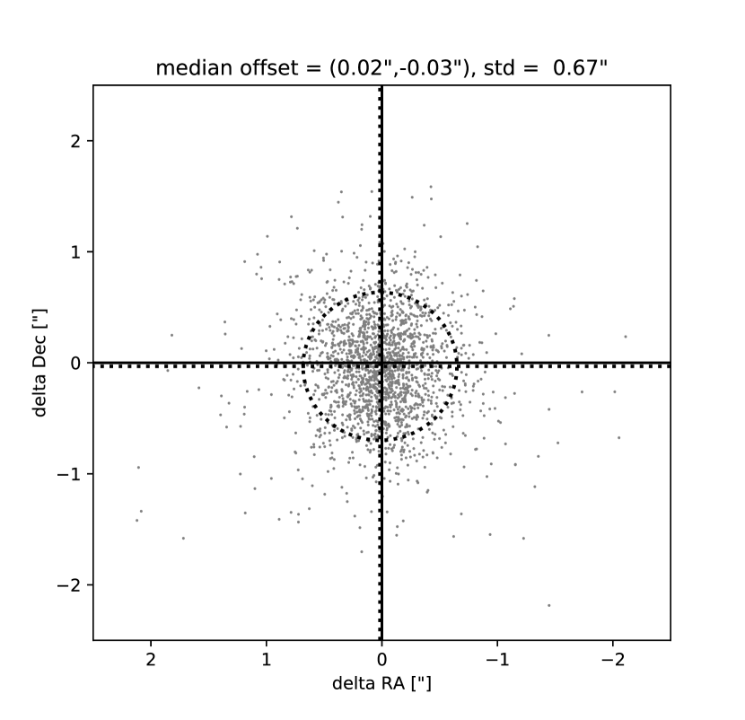
Figure 1: Positional offsets of bright, compact sources in overlapping pointings. The median offsets in RA and Dec are indicated by the vertical and horizontal lines, respectively, while the dotted circle represents the $1\sigma$ deviation (also indicated at the top).

3.2 Flux density corrections

To correct the individual pointing maps for primary beam attenuation, we adopt a standard, parameterised axisymmetric model, with coefficients given in the GMRT Observer Manual. Given the small fractional bandwidth covered (5.25%), we use the central frequency (610 MHz) beam model for all frequency channels. In Fig. 2 we show the ratio of the flux densities of the sources in overlapping pointings, but at various distances from the phase centres, not corrected for primary beam attenuation (hereafter apparent flux densities) as a function of the ratio of the primary beam model attenuations for the same sample of compact sources in overlapping pointings. For a perfect primary beam attenuation model the ratio of the apparent flux densities should be in one-to-one correspondence with the given ratio of the primary beam model attenuations. From Fig. 2 it is apparent that this is the case within a few percent on average, thus verifying the primary beam attenuation model used.

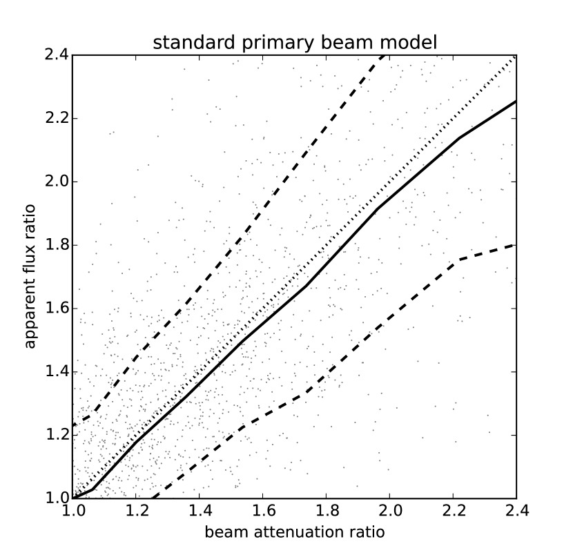
Figure 2: Ratio of apparent flux density (i.e., not corrected for primary beam attenuation; dots) vs. ratio of the primary beam model attenuations for a sample of bright, compact sources in overlapping pointings. The median and $\pm 1\sigma$ offsets are indicated by the full and dashed lines, respectively. The one-to-one line is represented by the dotted line.

Following Intema et al. (2016) we also quantify and apply antenna pointing corrections. In the top panel of Fig. 3 we show the ratio of flux densities of our sources in overlapping pointings as a function of the local azimuth of the source position in the first pointing. We account for the deviation from unity (changing sign at about 170 degrees), and in the bottom panel of Fig. 3 we show the corrected flux density ratios, now consistent with unity. We note that the $1\sigma$ scatter of the flux density ratios is $\sim 20\%$. As shown in Fig. 4 this value remains constant as a function of flux density. As the sources used for this analysis have been drawn from overlapping parts of various pointings, i.e. from areas further away from the pointing phase centres, where the $\rm{rms}$ noise is higher and the primary beam corrections less certain (see Fig. 2), this value should be taken as an upper limit on the relative uncertainty of the source flux densities.

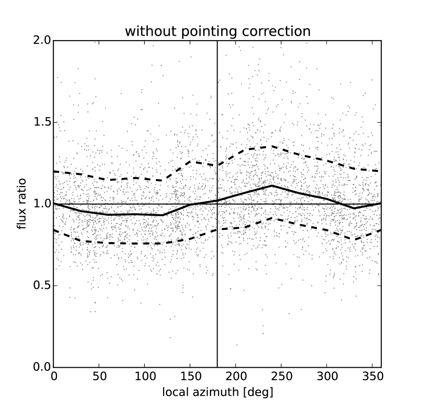
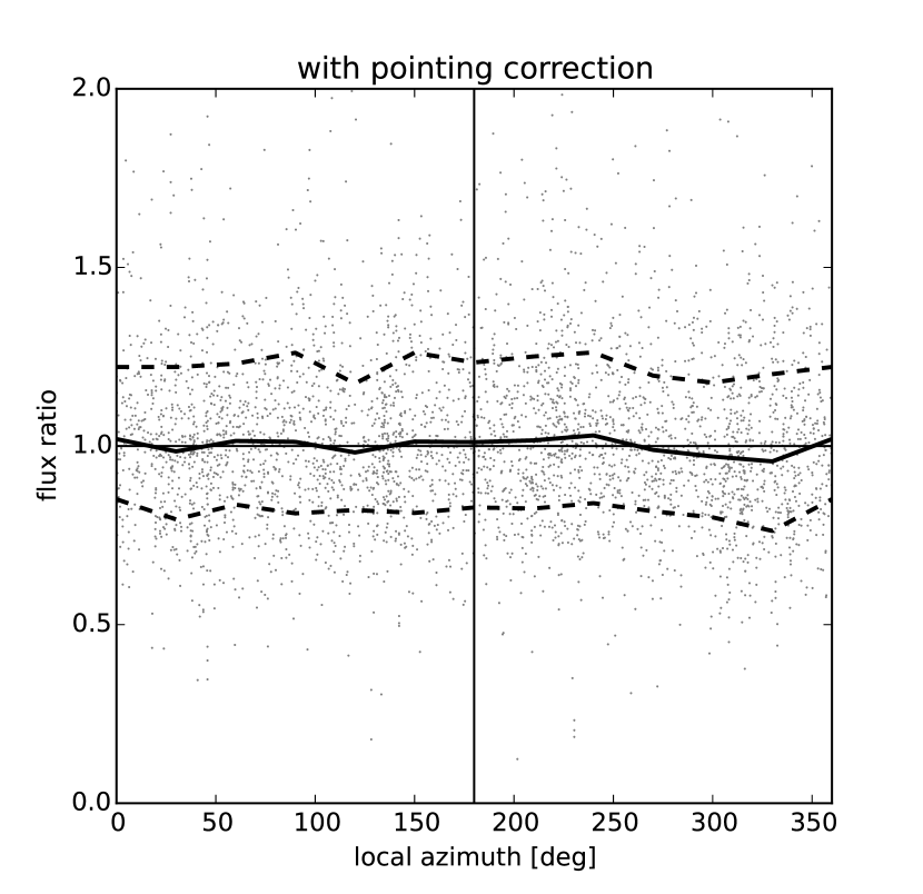
Figure 3: Ratio of flux densities (dots) of bright, compact sources in overlapping pointings as a function of local azimuth of the source position in the first pointing before (top) and after (bottom) applying the pointing correction (see text for details). In both panels the median and $\pm 1\sigma$ deviations are indicated by the full, and dashed lines, respectively.

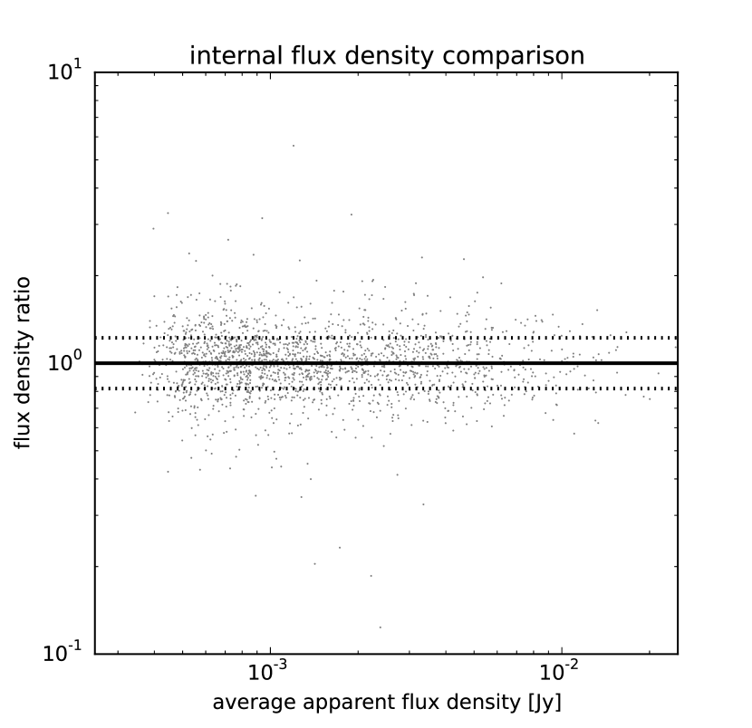
Figure 4: Ratio of flux densities (dots) of bright, compact sources in overlapping pointings as a function of their mean apparent flux density (i.e. uncorrected for primary beam attenuation). The median and $\pm 1\sigma$ is indicated by the full and dotted lines, respectively.

3.3 Final mosaic

After applying the per-pointing astrometric and flux density corrections described above to the individual pointings, each pointing (including its clean component and residual maps) is convolved to a common circular resolution of FWHM $6.5\arcsec\times 6.5\arcsec$, prior to mosaicing. This corresponds to a clean beam size larger than or equal to that intrinsically retrieved for the majority of the imaged pointings. The maps are then regridded to $1.9\arcsec\times 1.9\arcsec$ pixels, and combined into a mosaic in such a way that each pixel is weighted as the inverse square of the local rms, estimated using a circular sliding box with a 91-pixel diameter, chosen as a trade-off between minimising false detections at sharp boundaries between high noise and low noise, and separating extended emission regions from high rms regions. The final mosaic, shown in Fig. 5, containing $16,177\times 11,493$ pixels, encompasses a total area of $30.4$ square degrees. As can be seen in Fig. 5, the rms within the mosaic is highly non-uniform: It decreases from about 200 $\mu$Jy/beam within the XMM-LSS subregion, to about 50 $\mu$Jy/beam in the remaining area. Although a factor of 3.8 difference in sensitivity is significant, we note that the data processing applied here achieved a background noise reduction of 50% in the XMM-LSS area relative to the previous data release ($rms\sim 300\leavevmode\nobreak\ \mu$Jy/beam; Tasse et al. 2007). For comparison, in Fig. 6 we show the image of the central part of the XMM-LSS area of the XXL-N field obtained here, and within the previous data release (Tasse et al., 2007).

The overall areal coverage of the GMRT-XXL-N mosaic as a function of rms is shown in Fig. 7. For 60% of the total 30.4 square degree area an rms better than 150 $\mu$Jy/beam is achieved (with a median value of about 50 $\mu$Jy/beam). For the remainder (corresponding to the XMM-LSS subarea of the XXL-N field) a median rms of about 200 $\mu$Jy/beam is achieved.

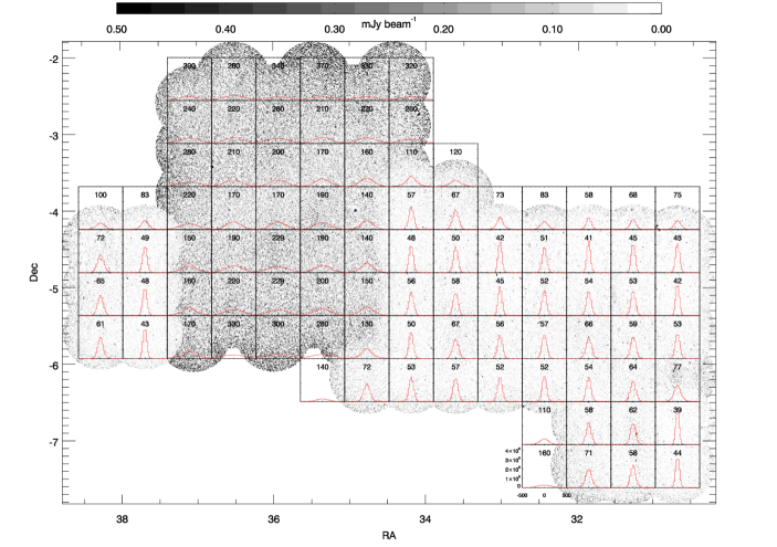
Figure 5: Grayscale mosaic with overlayed pixel flux distributions within small areas, encompassed by the panel (the local rms in $\mu$Jy/beam is indicated in each panel). The x and y ranges for all the panels are indicated in the bottom left panel.

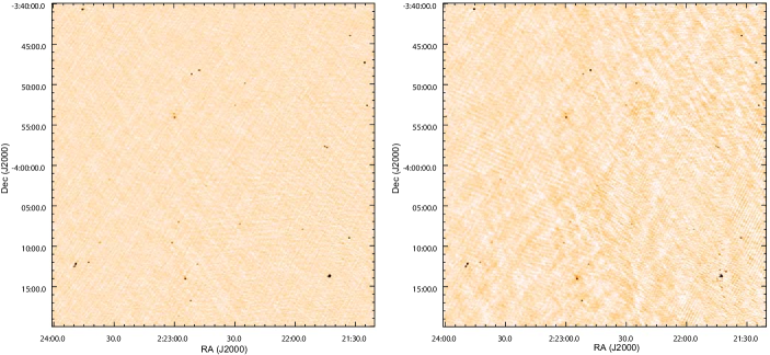
Figure 6: Mosaiced images of the XMM-LSS area of the XXL-N field obtained by the procedure presented here (left panel) and previously published (right panel; Tasse et al. 2007), using the same colour scale.

Figure 7: Areal coverage as a function of the rms noise in the mosaic.

4 Cataloguing

We describe the source extraction (Sect. 4.1), corrections performed to account for bandwidth smearing, and the measurement of the flux densities of resolved and unresolved sources (Sect. 4.2). We also describe the process of combining multiple detections, physically associated with single radio sources (Sect. 4.3), and present the final catalogue (Sect. 4.4).

4.1 Source extraction

To extract sources from our mosaic we used the PyBDSF software (Mohan & Rafferty, 2015). We set PyBDSF to search for islands of pixels with flux density values greater than or equal to three times the local rms noise (i.e $\geq 3\sigma$) surrounding peaks above $5\sigma$. To estimate the local rms a box of 195 pixels per side was used, leading to a good trade-off between detecting real objects and limiting false detections (see Sect. 5.2). Once islands are located, PyBDSF fits Gaussian components, and their flux density is estimated after deconvolution of the clean beam. These components are grouped into single sources when necessary, and final source flux densities are reported, as well as flags indicating whether multiple Gaussian fits were performed. The procedure resulted in 5 434 sources with signal-to-noise ratios $\geq 7$.

4.2 Resolved and unresolved sources and smearing

To estimate smearing due to bandwidth- and time-averaging, and to separate resolved from unresolved sources we follow the standard procedure, which relies on a comparison of the sources’ total and peak flux densities (e.g., Bondi et al., 2008; Intema, 2014; Smolčić et al., 2017a). In Fig. 8 we show the ratio of the total and peak flux densities ($S_{\mathrm{T}}$ and $S_{\mathrm{P}}$, respectively) for the 5 434 sources as a function of the signal-to-noise ratio ($\mathrm{S/N}\geq 7$). While the increasing spread of the points with decreasing S/N ratio reflects the noise properties of the mosaic, smearing effects will be visible as a systematic, positive offset from the $S_{\mathrm{T}}/S_{\mathrm{P}}=1$ line as they decrease the peak flux densities, while conserving the total flux densities. To quantify the smearing effect we fit a Gaussian to the logarithm of the $S_{\mathrm{T}}/S_{\mathrm{P}}$ distribution obtained by mirroring the lower part of the distribution over its mode (to minimise the impact of truly resolved sources). We infer a mean value of 6%, and estimate an uncertainty of 1% based on a range of binning and S/N ratio selections. After correcting the peak flux densities for this effect we fit a lower envelope encompassing 95% of the sources below the $S_{\mathrm{T}}/S_{\mathrm{P}}=1$ line, and mirror it above this line. Lastly, we consider all sources below this curve, of the form

$$S_{\mathrm{T}}/S_{\mathrm{P}}=1+3.2\times(S/N)^{-0.9},$$ (1)

as unresolved and set their total flux densities equal to their peak flux densities (corrected for the smearing effects). We note that the four extreme outliers ($S_{\mathrm{T}}/S_{\mathrm{P}}<0.5$) are due to blending issues, a locally high rms, or being possibly spurious.

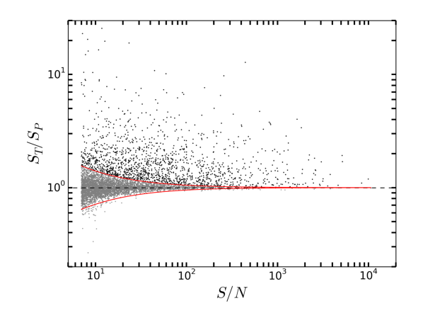
Figure 8: Total ($S_{\mathrm{T}}$) over peak ($S_{\mathrm{P}}$) flux as a function of signal-to-noise ratio. The horizontal dashed line shows the $S_{\mathrm{T}}/S_{\mathrm{P}}=1$ line. The upper curve was obtained by mirroring the lower curve (which encompasses 95% of the sources below the $S_{\mathrm{T}}/S_{\mathrm{P}}=1$ line; see Eq. 1) over the $S_{\mathrm{T}}/S_{\mathrm{P}}=1$ line. All sources below the upper curve are considered unresolved, while those above are considered resolved (see text for details).

4.3 Complex sources

Radio sources appear in many shapes, and it is possible that sources with complex radio morphologies (e.g. core, jet, and lobe structures that may be warped or bent) are listed as multiple sources within the source extraction procedure. To identify these sources we adopt the procedure outlined in Tasse et al. (2007). We identify groups of components within a radius of $60\arcsec$ from each other. Based on the source density in the inner part of the field, the Poisson probability is 0.22 $\%$ that two components are associated by chance. For the outer part of the field, an additional flux limit of $S_{\mathrm{610MHz}}>1.4$ mJy is imposed on the components prior to identifying the groups they belong to. This flux limit is justified by the size-flux relation for radio sources (e.g. Bondi et al., 2003), i.e. brighter sources are larger in size and are thus more likely to break into multiple components, and it also assures a Poisson probability of 0.39 $\%$ for a chance association. All of these groups were visually checked a posteriori, and verified against an independent visual classification of multicomponent sources performed by six independent viewers. In total we identify 768 sources belonging to 337 distinct groups of multiple radio detections likely belonging to a single radio source (see also next section).

4.4 Final catalogue

In our final catalog for each source we report the following:

• Column 1: Source ID;

• Columns 2-5: RA and Dec position (J2000) and error on the position as provided by PyBDSF;

• Column 6: Peak flux density ($S_{\mathrm{P}}$) in units of Jy/beam, corrected for smearing effects as detailed in Sect. 4.2;

• Column 7: Local rms value in units of Jy/beam;

• Column 8: S/N ratio;

• Column 9 - 10: Total flux density ($S_{\mathrm{T}}$) and its error, in units of Jy;

• Column 11: Flag for resolved sources; 1 if resolved, 0 otherwise. We note that the total flux density for unresolved sources equals the smearing corrected peak flux and the corresponding error lists rms scaled by the correction factor (see Sect. 4.2 for details);

• Column 12: Complex source identifier, i.e., ID of the group obtained by automatic classification of multicomponent sources (see Sect. 4.3 for details); if 0 no group associated with the source, otherwise the integer corresponds to the group ID;

• Column 13: Spectral index derived using the 610 MHz and 1.4 GHz (NVSS) flux densities, where available (-99.99 otherwise);

• Column 14: Area flag; $0$ if the source is in the inner mosaic area (within the XMM-LSS field and with higher rms), $1$ if it is in the outer field area (with better rms; see Sect. 3.3 and Fig. 5 for details);

• Column 15: Edge flag; 0 if the source is on the edge where the noise is high, $1$ otherwise. We note that selecting this flag to be 1 in the inner (outer) area, i.e. for area flag 0 (1) selects sources within areas of 7.7 (12.66) square degrees, while the area corresponds to 9.63 square degrees for the inner area (area flag 0) and an edge flag of 0 or 1.

The full catalogue is available as a queryable database table (XXL$\_$GMRT$\_$17) via the XXL Master Catalogue browser. A copy will also be deposited at the Centre de Données astronomiques de Strasbourg (CDS).

5 Reliability and completeness

In this section we assess the astrometric accuracy and false detection rate within the catalogue presented above (Sect. 5.1 and Sect. 5.2, respectively). We compare the source flux densities to those derived from the previous XMM-LSS GMRT 610 MHz data release (Sect. 5.3). We then derive average 610 MHz – 1.4 GHz spectral indices for unbiased subsamples of bright sources (Sect. 5.4), and use these to construct 1.4 GHz radio source counts, which we compare to counts from much deeper radio continuum surveys and thereby assess and quantify the incompleteness of our survey as a function of flux density (Sect. 5.5).

5.1 Astrometric accuracy

To assess the astrometric accuracy of the presented mosaic and catalogue, we compared the positions of our compact sources with those given in the FIRST survey. Using a search radius of $5\arcsec$ we found 1 286 matches. The overall median offset is (as expected) small ($\Delta\mathrm{RA}=-0.01\arcsec$, $\Delta\mathrm{Dec}=0.01\arcsec$), and the 1$\sigma$ position scatter radius is $0.62\arcsec$. This is similar to the internal positional accuracy seen in pointing overlap regions, and corresponds to roughly one-tenth of the angular resolution in the mosaic ($6.5\arcsec$).

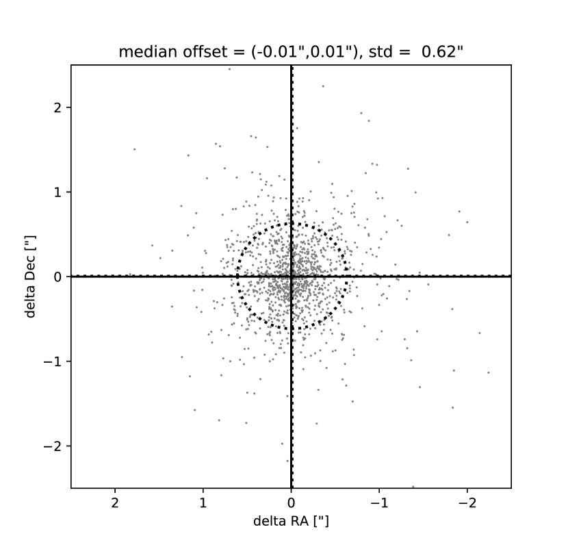
Figure 9: Positional offsets of sources detected in the XXL mosaic, relative to those catalogued within the FIRST survey. The median offsets in RA and Dec are indicated by the vertical and horizontal lines, respectively, while the dotted circle represents the $1\sigma$ deviation (also indicated at the top).

5.2 False detection rate

To assess the false detection rate, i.e. estimate the number of spurious sources in our catalogue, we ran PyBDSF on the inverted (i.e. multiplied by $-1$) mosaic. Each ’detection’ in the inverted mosaic can be considered spurious as no real sources exist in the negative part of the mosaic. Running PyBDSF with the same set-up as for the catalogue presented in Sect. 4 , we found only one detection with S/N ratio $\geq 7$ in the inverted mosaic. Since there are 5 434 detections with $\mathrm{S/N}\geq 7$ in the real mosaic, false detections are not significant ($<10^{-3}$ of the source population).

5.3 Flux comparison within the XMM-LSS area

We compared the flux densities for our sources extracted within the XMM-LSS area of the XXL-N field with those extracted in the same way, but over the XMM-LSS mosaic published by Tasse et al. (2007). Using a search radius of $5\arcsec$ we find 924 sources common to the two catalogues. In Fig. 10 we compare the PyBDSF-derived flux densities (prior to corrections for bandwidth smearing, and total flux densities). Overall, we find good agreement, with an average offset of 2.4%. This can be due to the use of different flux standards (Perley & Butler 2013 and Scaife & Heald 2012). We note that the comparison remains unchanged if flux densities from the Tasse et al. (2007) catalogue are used instead.

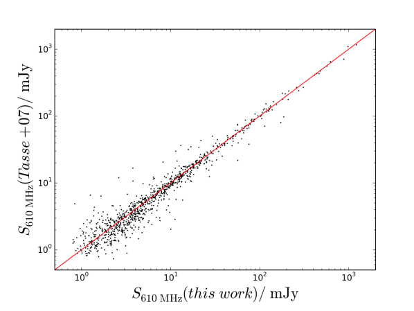
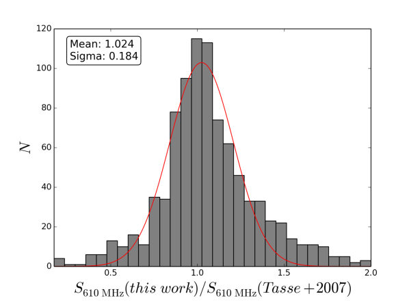
Figure 10: Comparison within the XMM-LSS area of the XXL-N field between the flux densities obtained here (x-axis) and those extracted in the same way, but over the mosaic published by Tasse et al. (2007, y-axis; top panel). The solid line is the diagonal. The distribution of the flux ratio, with fitted Gaussian is shown in the bottom panel.

5.4 Spectral indices

We derived the 610 MHz – 1.4 GHz spectral indices for the sources in our catalogue that are also detected in the the NVSS survey (Condon et al., 1998). We found 1 395 associations (470 within the XMM-LSS subarea) using a search radius of $20\arcsec$, which corresponds to about half of the NVSS synthesised beam (FWHM $\sim 45\arcsec$), and assures minimal false matches. In Fig. 11 we show the derived spectral indices as a function of 610 MHz flux density, separately for the XMM-LSS and the outer XXL areas (given the very different rms reached in the two areas). The different source detection limits of the NVSS and GMRT-XXL-N surveys would bias the derived spectral indices if taken at face value. Thus, to construct unbiased samples we defined flux density cuts of $S_{\mathrm{610MHz}}\geq 20$ mJy and $\geq 2$ mJy for the XMM-LSS, and outer XXL areas, respectively. As illustrated in Fig. 11, these cuts conservatively assure samples with unbiased $\alpha$ values. For samples defined in this way we find average spectral indices of -0.65 and -0.75 with standard deviations of 0.36 and 0.34, respectively. The values correspond to typically observed spectral indices of radio sources at these flux levels (e.g., Condon, 1992; Kimball & Ivezić, 2008), and they are consistent with those inferred by Tasse et al. (2007) based on the previous (XMM-LSS) data release.

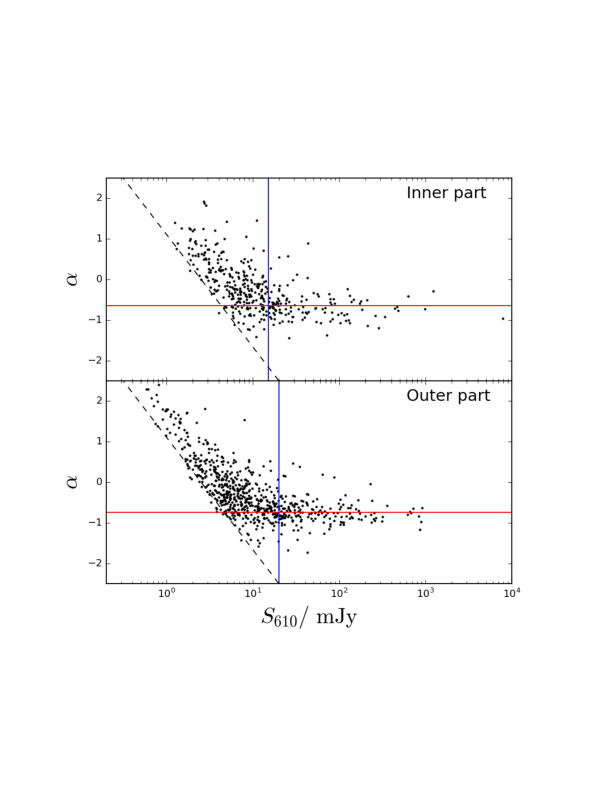
Figure 11: Spectral index based on 610 MHz and 1.4 GHz (NVSS) data ($\alpha$) as a function of 610 MHz flux density, separately shown for the XMM-LSS (top panel), and outer XXL-N (bottom panel) areas. The dashed line in both panels indicates the constraint on $\alpha$ placed by the NVSS detection limit (2.5 mJy), and the vertical full line indicates the threshold beyond which the sample is not expected to be biased by the different detection limits. The horizontal line indicates the average spectral index for sources with flux densities above this threshold.

5.5 Source counts and survey incompleteness

In Fig. 12 we show the Euclidean normalised source counts at 1.4 GHz frequency derived for our GMRT-XXL-N survey, separately for the inner (XMM-LSS) and outer XXL-N areas. We have chosen a reference frequency of 1.4 GHz for easier comparison with the counts from the literature, which are deeper than our data and are based on data and on simulations (Condon, 1984; Wilman et al., 2008; Smolčić et al., 2017a). The 610 MHz flux densities were converted to 1.4 GHz using a spectral index of $\alpha=-0.7$, as derived in the previous section. The area considered for deriving the GMRT-XXL-N counts within the inner (XMM-LSS) area (with an rms of $\sim 200\leavevmode\nobreak\ \mu$Jy/beam) was 9.6 square degrees (green symbols in Fig. 12). Two areas were considered for the outer XXL-N region: the full area of 20.75 square degrees (also containing the noisy edges; see Fig. 5) and an area of 12.66 square degrees, which excludes the noisy edges and is characterised by a fairly uniform rms of $\sim 45\leavevmode\nobreak\ \mu$Jy/beam (black and yellow symbols, respectively, in Fig. 12). We find that the counts within these 12.66 square degrees are $40-60$% higher than those derived using the full outer area (below 0.4 mJy). This suggests that including the noisy edges (as would be expected) further contributes to survey incompleteness; hereafter we thus only consider the 12.66 square degree area for the outer GMRT-XXL-N field.

In Fig. 12 we also show the 1.4 GHz counts derived by Condon (1984), Wilman et al. (2008) and Smolčić et al. (2017a). Condon (1984) developed a model for the source counts using the local 1.4 GHz luminosity function for two dominant, spiral and elliptical galaxy populations combined with source counts, redshift, and spectral-index distributions for various 400 MHz to 5 GHz flux limited samples. The Square Kilometre Array Design Study (SKADS) simulations of the radio source counts were based on evolved luminosity functions of various radio populations, also accounting for large-scale clustering (Wilman et al., 2008). Lastly, the counts taken from Smolčić et al. (2017a) were constructed using the VLA-COSMOS 3 GHz Large Project, to date the deepest ($\mathrm{rms}\sim 2.3\leavevmode\nobreak\ \mu$Jy/beam) radio survey of a relatively large field (2 square degrees). Their 1.4 GHz counts were derived using the average spectral index ($\alpha=-0.7$) inferred for their 3 GHz sources. We note that the various counts from the literature are consistent down to the flux level reached by our GMRT-XXL-N data ($\sim 0.15\leavevmode\nobreak\$mJy), and that they are in good agreement with our GMRT counts down to $\sim 2$ mJy, implying that our survey is complete at 1.4 GHz flux densities $>2$ mJy. This corresponds to 610 MHz flux densities of $>4$ mJy, beyond which we take the detection fractions and completeness to equal unity (see below).

The decline at 1.4 GHz (610 MHz) flux densitites $\lesssim 2$ mJy ($\lesssim 4$ mJy) of the derived GMRT-XXL-N counts, compared to the counts from the literature (see Fig. 12) , can be attributed to the survey incompleteness. In radio continuum surveys this is due to a combination of effects, such as real sources remaining undetected due to their peak brightnesses falling below the detection threshold given the noise variations across the field, or source extendedness, and the flux densities of those detected being over- or underestimated due to these noise variations. Commonly, such survey incompleteness is accounted for by statistical corrections (as a function of flux density) taking all these combined effects into account (e.g. Bondi et al., 2008; Smolčić et al., 2017a). The approach we take here makes use of the availability of radio continuum surveys that reach much deeper than our GMRT-XXL-N 610 MHz survey. In particular, for the inner (XMM-LSS; 9.6 square degrees, $\mathrm{rms}\sim 200\leavevmode\nobreak\ \mu$Jy/beam) and outer (12.66 square degrees, $\mathrm{rms}\sim 45\leavevmode\nobreak\ \mu$Jy/beam) GMRT-XXL-N areas, we derive the measurements relative to the VLA-COSMOS 3 GHz source counts. The $\sim 2.3\leavevmode\nobreak\ \mu$Jy/beam depth of the VLA-COSMOS 3 GHz Large Project means these counts are 100% complete in the flux regime encompassed by the GMRT-XXL-N survey (see Smolčić et al. 2017a for details).

The GMRT-XXL-N survey differential incompleteness measurements (i.e. detection fractions as a function of flux density) are computed as the ratio of the GMRT-XXL-N and VLA-COSMOS source counts, are shown in Fig. 13, and listed in Tab. 1 separately for the inner and outer areas of the mosaic. The listed corrections, combined with the ’edge flag’, given in the catalogue (see Sect. 4.4), can be used to statistically correct for the incompleteness of the source counts important to determine luminosity functions. In Fig. 13 we also show the total completeness of the survey within the given areas corresponding to the fraction of sources detected above the given flux bin (lower) limit; in Fig. 14 we show the same, but for the full 30.4 square degree mosaic. We note that we consider the survey complete beyond $S_{\mathrm{610MHz}}=4.6$ mJy, below which the detection fraction decreases. The overall completeness for the full area (30.4 square degree survey) reaches 50% at $S_{\mathrm{610MHz}}\approx 400\leavevmode\nobreak\ \mu$Jy (i.e. about $250\leavevmode\nobreak\ \mu$Jy in the outer XXL area and about $900\leavevmode\nobreak\ \mu$Jy in the inner XXL area). Furthermore, comparing the detection fraction derivation with that derived relative to the SKADS simulation, we estimate a possible uncertainty of the derived values of the order of 10%.

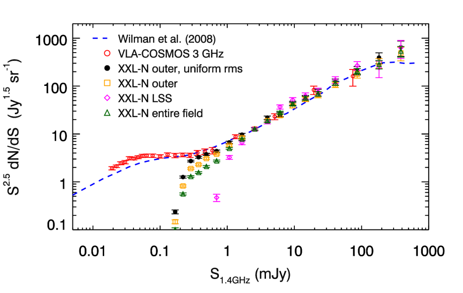
Figure 12: Source counts at 1.4 GHz , normalised to Euclidean space separately for various surveys (symbols) and simulations (lines), as indicated in the panel. The 610 MHz flux densities have been translated to 1.4 GHz using a spectral index of $\alpha=-0.7$, as derived in Sect. 5.4. The rapid decline of the GMRT-XXL-N counts (at $S_{\mathrm{1.4GHz}}<2$ mJy) is due to survey incompleteness (see text for details).

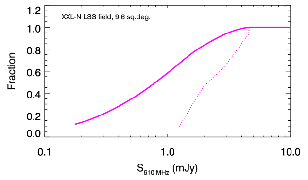
Figure 13: Detection fraction as a function of 610 MHz flux density relative to the VLA-COSMOS 3 GHz Large Project (dashed line) for the inner area (9.6 square degrees, coincident with the XMM-LSS field; left panel) and outer area (12.66 square degree) areas. Also shown is the completeness (i.e. the detection fraction in a given bin and that above the given flux bin lower limit) as a function of flux density (full line).

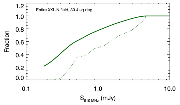
Figure 14: Same as Fig. 14 but for the full 30.4 square degree observed GMRT-XXL-N area.

Table 1: Differential incompleteness measures, i.e. detection fraction as a function of 610 MHz flux density for the GMRT-XXL-N 610 MHz survey relative to the VLA-COSMOS 3 GHz Large Project source counts, and separated into two areas (inner and outer field) with different $1\sigma$ sensitivity limits. The estimated uncertainty of the detection fractions computed in this way is $\sim 10\%$. Beyond the flux densities given here, we consider the survey complete (see text for details).

inner area	(9.6 deg2)	outer area	(12.66 deg2)
$S_{\mathrm{610MHz}}$	detection	$S_{\mathrm{610MHz}}$	detection
$[$mJy$]$	fraction	$[$mJy$]$	fraction
1.92	0.45	0.39	0.34
2.96	0.65	0.51	0.75
4.58	0.94	0.67	0.80
		0.87	0.87
		1.24	0.87
		1.92	0.92
		2.96	0.96
		4.58	0.95

6 Summary and conclusions

Based on a total of 192 hours of observations with the GMRT towards the XXL-N field we have presented the GMRT-XXL-N 610 MHz radio continuum survey. Our final mosaic encompasses a total area of 30.4 square degrees with a non-uniform rms, being $\sim 200\leavevmode\nobreak\ \mu$Jy/beam in the inner area (9.6 square degrees) within the XMM-LSS field, and $\sim 45\leavevmode\nobreak\ \mu$Jy/beam in the outer area (12.66 square degrees). We have presented a catalogue of 5 434 radio sources with S/N ratios down to $7\times$ rms. Of these, 768 have been identified as components of 337 larger sources with complex radio morphologies, and flagged in the final catalogue. The astrometry, flux accuracy, false detection rate and completeness of the survey have been assessed and constrained.

The derived 1.4 GHz radio source counts reach down to flux densities of $\sim 150\leavevmode\nobreak\ \mu$Jy (corresponding to $\sim 290\leavevmode\nobreak\ \mu$Jy at 610 MHz frequency assuming a spectral index of $\alpha=-0.7$, which is consistent with the average value derived for our sources at the bright end). Past studies have shown that the radio source population at these flux densities is dominated by AGN, rather than star forming galaxies (e.g. Wilman et al., 2008; Padovani et al., 2015; Smolčić et al., 2008, 2017a). This makes the GMRT-XXL-N 610 MHz radio continuum survey, in combination with the XXL panchromatic data a valuable probe for studying the physical properties, environments, and cosmic evolution of radio AGN.

References

- Becker et al. (1995) Becker, R. H., White, R. L., & Helfand, D. J. 1995, ApJ, 450, 559
- Best et al. (2014) Best, P. N., Ker, L. M., Simpson, C., Rigby, E. E., & Sabater, J. 2014, MNRAS, 445, 955
- Bock et al. (1999) Bock, D. C.-J., Large, M. I., & Sadler, E. M. 1999, AJ, 117, 1578
- Bondi et al. (2008) Bondi, M., Ciliegi, P., Schinnerer, E., et al. 2008, ApJ, 681, 1129
- Bondi et al. (2003) Bondi, M., Ciliegi, P., Zamorani, G., et al. 2003, A&A, 403, 857
- Butler et al. (2017) Butler, A., XXX, M., XXX, M., XXX, P., & XXX, K. P. 2017, A&A, 602, A1 (XXL Paper XVIII)
- Condon (1984) Condon, J. J. 1984, ApJ, 284, 44
- Condon (1992) Condon, J. J. 1992, ARA&A, 30, 575
- Condon et al. (1998) Condon, J. J., Cotton, W. D., Greisen, E. W., et al. 1998, AJ, 115, 1693
- Croton et al. (2006) Croton, D. J., Springel, V., White, S. D. M., et al. 2006, MNRAS, 365, 11
- Croton et al. (2016) Croton, D. J., Stevens, A. R. H., Tonini, C., et al. 2016, ApJS, 222, 22
- Donoso et al. (2009) Donoso, E., Best, P. N., & Kauffmann, G. 2009, MNRAS, 392, 617
- Heckman & Best (2014) Heckman, T. M. & Best, P. N. 2014, ARA&A, 52, 589
- Intema (2014) Intema, H. T. 2014, ArXiv e-prints
- Intema et al. (2016) Intema, H. T., Jagannathan, P., Mooley, K. P., & Frail, D. A. 2016, ArXiv e-prints
- Intema et al. (2009) Intema, H. T., van der Tol, S., Cotton, W. D., et al. 2009, A&A, 501, 1185
- Kimball & Ivezić (2008) Kimball, A. E. & Ivezić, Ž. 2008, AJ, 136, 684
- Mohan & Rafferty (2015) Mohan, N. & Rafferty, D. 2015, PyBDSM: Python Blob Detection and Source Measurement, Astrophysics Source Code Library
- Padovani (2016) Padovani, P. 2016, A&A Rev., 24, 13
- Padovani et al. (2015) Padovani, P., Bonzini, M., Kellermann, K. I., et al. 2015, ArXiv e-prints
- Perley & Butler (2013) Perley, R. A. & Butler, B. J. 2013, ApJS, 204, 19
- Pierre et al. (2016) Pierre, M., Pacaud, F., Adami, C., et al. 2016, A&A, 592, A1 (XXL Paper I)
- Pracy et al. (2016) Pracy, M. B., Ching, J. H. Y., Sadler, E. M., et al. 2016, MNRAS, 460, 2
- Sadler et al. (2007) Sadler, E. M., Cannon, R. D., Mauch, T., et al. 2007, MNRAS, 381, 211
- Scaife & Heald (2012) Scaife, A. M. M. & Heald, G. H. 2012, MNRAS, 423, L30
- Smolčić (2009) Smolčić, V. 2009, ApJ, 699, L43
- Smolčić et al. (2016) Smolčić, V., Delhaize, J., Huynh, M., et al. 2016, A&A, 592, A10 (XXL Paper XI)
- Smolčić et al. (2017a) Smolčić, V., Novak, M., Bondi, M., et al. 2017a, A&A, 699, 24
- Smolčić et al. (2017b) Smolčić, V., Novak, M., Delvecchio, I., et al. 2017b, A&A, 602, A6
- Smolčić et al. (2008) Smolčić, V., Schinnerer, E., Scodeggio, M., et al. 2008, ApJS, 177, 14
- Smolčić et al. (2009) Smolčić, V., Zamorani, G., Schinnerer, E., et al. 2009, ApJ
- Tasse et al. (2006) Tasse, C., Cohen, A. S., Röttgering, H. J. A., et al. 2006, A&A, 456, 791
- Tasse et al. (2007) Tasse, C., Röttgering, H. J. A., Best, P. N., et al. 2007, A&A, 471, 1105
- Willott et al. (2001) Willott, C. J., Rawlings, S., Blundell, K. M., Lacy, M., & Eales, S. A. 2001, MNRAS, 322, 536
- Wilman et al. (2008) Wilman, R. J., Miller, L., Jarvis, M. J., et al. 2008, MNRAS, 388, 1335