Resampling Strategies to Improve Surrogate Model-based Uncertainty Quantification - Application to LES of LS89.

Abstract

[Abstract] Uncertainty Quantification (UQ) is receiving more and more attention for engineering applications in particular from robust optimization. Indeed, running a computer experiment only provides a limited knowledge in terms of uncertainty and variability of the input parameters. These experiments are often computationally expensive and surrogate models can be constructed to address this issue. The outcome of a UQ study is in this case directly correlated to the surrogate’s quality. Thus, attention must be devoted to the Design of Experiments (DoE) to retrieve as much information as possible. This work presents two new strategies for parameter space resampling to improve a Gaussian Process surrogate model. These techniques indeed show an improvement of the predictive quality of the model with high dimensional analytical input functions. Finally, the methods are successfully applied to a turbine blade Large Eddy Simulation application: the aerothermal flow around the LS89 blade cascade.

, , , and (2018), Resampling Strategies to Improve Surrogate Model-based Uncertainty Quantification - Application to LES of LS89., International Journal for Numerical Methods in Fluids, 2018;00:1-25, DOI: 10.1002/fld.4504.

1 Introduction

Design process and robust optimization are the major purposes of most engineering works dealing with Computational Fluid Dynamics (CFD), especially in aeronautical or automotive industry ¹. Despite the large amount of work that has been devoted to the design of efficient optimization techniques, the design process still requires important investments (financial and human) ². As a consequence, design errors appear after the industrialization phase ³ and the implications these can have may be critical. This partially explains why CFD tools have been used more and more in the past decades to decrease the number of iterations between conception and experiments to avoid irreversible errors during the preliminary design phase.

Nowadays, CFD codes have reached maturity and represent more accurately physical flow phenomena. Complex flow simulations on high-resolution grids are possible thanks to the continuous developments in numerical models and in High Performance Computing (HPC). Nevertheless, deterministic simulations only provide limited knowledge about a system. Uncertainties in the numerical model as well as in the problem formulation or inputs are necessarily present and translate into uncertainties in the outputs ⁴.

In fact, the diversity of uncertainties on the CFD boundary conditions or initial conditions, as well as on model parameters (input data, geometry, simplification of the model physics, etc.) limits the validity of the simulations: the quantity of interest (QoI) can be easily affected and shadowed by the conjugation of all types of uncertainties. This assessment explains why Uncertainty Quantification (UQ) is now becoming a mandatory step in application-oriented modelling for operational and industrial purposes ^{5, 6}. It provides insight into the level of uncertainty in the numerical simulation results but also gives access to the Sensitivity Analysis (SA) which aims at describing the respective influences of the input parameters on the QoI. The inclusion of UQ in a design optimization cycle hence allows manufacturers to design quicker and obtain better, cheaper and more robust (i.e. more stable) products.

Classical UQ methods, based on the Monte-Carlo approach, require a large number of CFD simulations ⁷, which quickly go beyond the limits of available computational resources (CPU cost). This is especially true when it comes to large dimensional problems, both with respect to the domain discretization and to the number of uncertain input parameters. The cost of the UQ study can however be significantly reduced when the CFD code is replaced by a surrogate model which is formulated in a parameter space and which is fast to evaluate at any set of uncertain variables ⁸.

Two successful approaches for building a surrogate model are Polynomial Chaos ⁹ and Gaussian Process ¹⁰. The approach used in this work consists in combining Gaussian Processes with Proper Orthogonal Decomposition (POD) to build response surfaces through interpolation ^{11, 12}. In an industrial context—which is the case here—, some benefits of this method are:(i) it does not require any prior knowledge on the probability distribution of the uncertainties on the input parameters ; (ii) it does not need a specific sampling of the parameter space which could lead to curse-of-dimensionality or mis-evaluation of the space ; (iii) it provides an estimation of the predictive error ; and (iv) the use of the POD reduces the number of predictors to compute. Details and comparisons can be found in ^{13, 14}.

In any case, the number of CFD simulations that is required for the formulation of the surrogate model is defined by the complexity of the physics and the number of input parameters to take into account. This factor is paramount when considering costly numerical simulations.

The accuracy of an uncertainty quantification being directly correlated to the quality of the surrogate ¹⁵, the present study aims at improving its construction by using two new strategies for resampling the parameter space. Industrial applications being targeted, a first UQ analysis of the LS89 case ¹⁶ using Large Eddy Simulation (LES) is presented. LES are high-fidelity full 3D unsteady simulations. This approach comes at a high CPU cost which requires the use of High Performance Computing (HPC) resources.

The paper is tailored as follows; Section 2 starts by presenting the techniques employed to construct the surrogate model as well as its error assessment. Then the UQ tools used are detailed and Section 3.1 describes the two proposed strategies. After this methodological presentation, Section 4 assesses the benefits of these strategies on several difficult analytical functions and presents the results on the application: the aerothermal analysis around the LS89 blade cascade. Finally, Section 5 will put a closure to this paper by summarizing its contributions along with potential directions for future works or applications.

2 Surrogate model for UQ

In this study, the surrogate model is created using the BATMAN (Bayesian Analysis Tool for Modeling and uncertAinty quaNtification) tool ¹⁴ which is written in Python language. Using a non-intrusive approach, BATMAN allows to construct a surrogate model from any black-box code. The result obtained is a POD-based Gaussian Process (pGP) surrogate which is computationally inexpensive and able to interpolate any new realization (or snapshot) $\mathbf{x_{*}}$ not in the sample composed of $N_{s}$ snapshots. BATMAN’s workflow is detailed in Algorithm 1.

Algorithm 1 POD-based Gaussian Process

1:Choose the size of the sample $N_{s}$

2:Pick $N_{s}$ samples in the input space $\mathbf{x}$ with a low discrepancy design of experiment (DoE)

3:Perform a POD on the output

4:Formulate the pGP surrogate $\mathcal{M}_{\text{gp}}$ on the POD’s coefficients

5:Resample the parameter space if necessary

All different steps are detailed in the following sections. Section 2.1 presents the POD technique and Section 2.2 reminds the Gaussian process technique. The quality of the surrogate is addressed in Section 2.3 and the UQ methods are detailed in Section 2.4. Finally, in order to improve the surrogate’s quality, resampling strategies are presented in Section 3.1. Figure 1 shows the workflow implemented in the BATMAN tool for constructing the surrogate model for UQ.

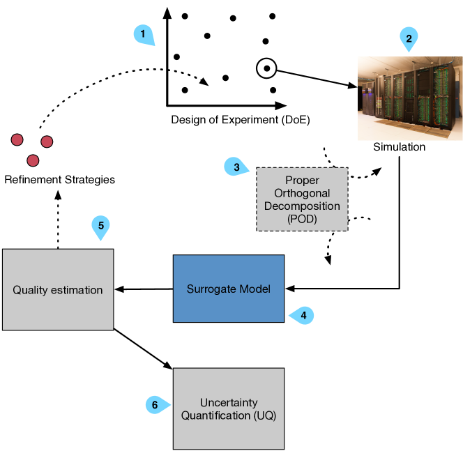
Figure 1: Workflow to resample the parameter space in an Uncertainty Quantification framework.

2.1 POD

A function $z$ can be approximate using a finite sum of terms:

$$z(m,N_{i}) \simeq\sum_{k}a_{k}(N_{i})\phi_{k}(x),$$ (1)

with $m$ being the spatial discretization and $N_{i}$ a realization of the code, a snapshot. The functions $\phi_{k}(m)$ have an infinite representation and can be Fourier series, Chebyshev polynomials, etc. For a chosen basis of functions, a set of unique snapshot functions $a_{k}(N_{i})$ arises. In the case of POD ¹⁷, the basis functions are orthonormal which implies:

$$(\phi_{k_{1}},\phi_{k_{2}}) =\left\{\begin{array}[]{rcl}1&\text{if}&k_{1}=k_{2}\\ 0&\text{if}&k_{1}\neq k_{2}\end{array}\right.,$$ (4)

$$a_{k}(N_{i}) =z(m,N_{i})\cdot\phi_{k}(m),$$

with $(\cdot,\cdot)$ the inner product. The principle of POD is to choose $\phi_{k}(m)$ such that the approximation of $z(m,N_{i})$ is optimal in a least square sense. These orthonormal functions are called the proper orthogonal modes of the function. Modes can be found using a Singular Value Decomposition (SVD) of the snapshot matrix ¹⁸. Considering the snapshot matrix $\mathbf{A}$, gathering the output QoI computed spatially on $m$ for the $N_{s}$ snapshots:

$$\mathbf{A}=\left[\mathbf{z}^{N_{1}},\cdots,\mathbf{z}^{N_{i}},\cdots,\mathbf{z}^{N_{S}}\right],$$ (5)

with $\mathbf{z}^{N_{i}}$ the i-th snapshot vector stored as a column in $\mathbf{A}$. The SVD is a factorization operation of a matrix expressed as:

$$\mathbf{A}=\mathbf{U}\mathbf{\Sigma}\mathbf{V}^{T},$$ (6)

with $\mathbf{V}\in\mathbb{R}^{N_{s}\times N_{s}}$ diagonalizes $\mathbf{A}^{T}\mathbf{A}$, $\mathbf{U}\in\mathbb{R}^{m\times m}$ diagonalizes $\mathbf{A}\mathbf{A}^{T}$ and $\mathbf{\Sigma}\in\mathbb{R}^{m\times N_{s}}$ is the singular value matrix with its diagonal composed by the singular values $\sigma$ of $\mathbf{A}$. Thus, the initial matrix can be rewritten:

$$\mathbf{A}=\sum_{i=1}^{r}\sigma_{i}u_{i}v_{i}^{T},$$ (7)

with $u_{i}$ and $v_{i}$ the eigen vectors of respectively $\mathbf{U}$ and $\mathbf{V}$ which form an orthonormal basis. Also $r=\min(m,N_{s})$ is the rank of the matrix. Due to the singular value matrix’s null terms, the reduced form of the matrices is used which leads to $\mathbf{U}\in\mathbb{R}^{m\times N_{s}}$, $\mathbf{\Sigma}\in\mathbb{R}^{N_{s}\times N_{s}}$. Note that one can apply a filtering on the modes to only keep the basis vectors containing the highest energy of the system. For any $k<r$, an optimal approximation of rank $k$ of the snapshot matrix $\mathbf{A}_{k}=\mathbf{U}\mathbf{\Sigma}_{k}\mathbf{V}^{T}_{k}$ can be calculated by setting the $\sigma_{i>k}=0$ in $\mathbf{\Sigma}$. These two steps allow to compress the data as only an extract of $\mathbf{U}$ and $\mathbf{\Sigma}$ need to be stored. But the real benefit is that a surrogate model does not need to be carried out for all points of the spatial discretization of the QoI but only for the matrix $\mathbf{\Sigma}_{k}\mathbf{V}^{T}_{k}$ (a column of this matrix corresponds to a snapshot).

2.2 The Gaussian Process Regression

A Gaussian Process (GP) is a collection of random variables which have a joint Gaussian distribution ¹⁰. GP is equivalent to Kriging ¹⁹. In this case, the random variable being the POD coefficients computed for each random input vector $\mathbf{x}$ of $N_{s}$: $f(\mathbf{x})=(\mathbf{\Sigma}_{k}\mathbf{V}^{T}_{k})_{\mathbf{x}}$. A new prediction consists in a new column of $\mathbf{\Sigma}_{k}\mathbf{V}^{T}_{k}$. A Gaussian Process $\mathcal{GP}$ is described by its mean $m(\mathbf{x})$ and covariance $k(\mathbf{x},\mathbf{x}^{\prime})$—where $\mathbf{x},\mathbf{x}^{\prime}$ are different sets of inputs

$$f(\mathbf{x}) \sim\mathcal{GP}(m(\mathbf{x}),k(\mathbf{x},\mathbf{x}^{\prime})),\;\text{with}$$ (8)

$$m(\mathbf{x}) =\mathbb{E}\left[f(\mathbf{x})\right],$$

$$k(\mathbf{x},\mathbf{x}^{\prime}) =\mathbb{E}\left[(f(\mathbf{x})-m(\mathbf{x}))(f(\mathbf{x}^{\prime})-m(\mathbf{x}^{\prime}))\right].$$

Here the covariance function $k$ (or kernel) is chosen as a squared exponential

$$K=k(\mathbf{x},\mathbf{x}^{\prime})=\sqrt{\pi}\;\sigma_{\mathbf{x}}^{2}\exp{-\frac{(\mathbf{x}-\mathbf{x}^{\prime})^{2}}{2(\sqrt{2}l)^{2}}},$$ (9)

where $l$ is a length scale that describes the trend in the data and $\sigma_{\mathbf{x}}$ is the variance of the output signal. Then the GP model consists of a regression providing an interpolation $\hat{f}$ for a new set of input parameters $\mathbf{x_{*}}$:

$$\hat{f}(\mathbf{x}_{*}) =\mathrm{bar}{f}(\mathbf{x}_{*})=\sum_{i=1}^{N_{s}}\alpha_{i}k(\mathbf{x}_{i},\mathbf{x}_{*}),\;\text{with}$$ (10)

$$\mathbf{\alpha} =(K+\sigma_{n}^{2}I)^{-1}\mathbf{y},$$

where $\mathrm{bar}{f}$ is the mean realization, $\mathbf{x}_{i}$ the i-th set of parameters, $\mathbf{y}$ the snapshot matrix and $\sigma_{n}$ is the variance of the input variables. Indeed, it is the mean realization of the conditioned process considering an artificial noisy observation which gives the prediction. The learning phase of the GP consists in selecting $l$, $\sigma_{n}$ and $\sigma_{\mathbf{x}}$ so that $f$ passes through or close to the dataset points. These hyperparameters are optimized using a differential evolution strategy. A key advantage of this predictor is that it provides an inference about its prediction variance

$$\mathbb{V}[f(\mathbf{x}_{*})]=k(\mathbf{x}_{*},\mathbf{x}_{*})-\mathbf{k}(\mathbf{x}_{*})^{T}(K+\sigma_{n}^{2}I)^{-1}\mathbf{k}(\mathbf{x}_{*}).$$ (11)

2.3 Estimation of the error

To correctly adapt the number of snapshots to the required precision, the quality of the model has to be evaluated by comparing expected values and their estimations. A common indicator is to compute the predictivity coefficient $Q_{2}$ ²⁰:

$$Q_{2}=1-\frac{\displaystyle\sum_{i=1}^{N_{s}}(f_{i}-\hat{f_{i}})^{2}}{\displaystyle\sum_{i=1}^{N_{s}}(f_{i}-\mathrm{bar}{f})^{2}},$$ (12)

with $\overline{f}$ denoting the mean value, $f_{i}$ the measured point and $\hat{f_{i}}$ its prediction by the model. When dealing with a non-analytical function the expected values are not known. However, there are two methods to evaluate the precision:

• The sample can be divided into a validation set and training set. The model is built based on the training set and then evaluations are compared relative to the validation set. However, this technique requires that we do not use the validation simulations which is computationally costly when dealing with high fidelity numerical experiments.

• Another approach is to estimate the quality by k-fold Cross Validation ²¹. A particular case is the Leave-One-Out Cross Validation (LOO) with $k=n=1$—with $n$ the number of observations. The LOO technique derived from statistical learning theory requires the formulation of several surrogates. Each surrogate is built excluding one point from the evaluation sample; the accuracy of the surrogate is then calculated at this particular point. Removing point $p$ from $\hat{f_{p}}$ gives $\hat{f_{p}}^{(-p)}$ and leads to an error

  $$\epsilon_{p} =\|f_{p}-\hat{f_{p}}^{(-p)}\|_{2}.$$ (13)

  with the Euclidean 2-norm considered for $\mathbb{R}^{m}$. This is done all over the sample composed of $N_{s}$ snapshots to get the mean-square-error

  $$LOO =\frac{1}{N_{s}}\sum_{p=1}^{N_{s}}\epsilon_{p}^{2}.$$ (14)

  Thus, an estimated predictivity coefficient $\hat{Q}_{2}$ can be retrieved

  $$\hat{Q}_{2}=1-\frac{LOO}{\displaystyle\sum_{p=1}^{N_{s}}\left(\hat{f}_{p}-\mathrm{bar}{\hat{f}}\right)^{2}}\quad.$$ (15)

As stated in ¹⁵, this estimation tends to be pessimistic. Indeed, a snapshot is removed from an already very small sample which ultimately tends to lower the predictive quality of the model. However the indicator is stable—provided a correct sample size ($N_{s}>10n_{dim}$, with $n_{dim}$ the number of dimension ²²)—and as the quality increases, the difference between the estimation and the real quality vanishes.

2.4 Uncertainty Quantification

There are several methods to estimate the contribution of different parameters on quantities of interest ²³. Among them, sensitivity methods based on the analysis of the variance allow to obtain the contribution of the parameters on the QoI’s variance ²⁴. Here, classical Sobol’ ²⁵ method is used which gives not only a ranking but also quantifies the importance factor using the variance. This method only makes the hypothesis of the independence of the input variables. It uses a functional decomposition of the variance of the function to explore:

$$\mathbb{V}(\mathcal{M}_{gp}) =\sum_{i}^{p}\mathbb{V}_{i}(\mathcal{M}_{gp})+\sum_{i<j}^{p}\mathbb{V}_{ij}+...+\mathbb{V}_{1,2,...,p},$$ (16)

$$\mathbb{V}_{i}(\mathcal{M}_{gp}) =\mathbb{\mathbb{V}}[\mathbb{E}(\mathcal{M}_{gp}|x_{i})]$$

$$\mathbb{V}_{ij} =\mathbb{\mathbb{V}}[\mathbb{E}(\mathcal{M}_{gp}|x_{i}x_{j})]-\mathbb{V}_{i}-\mathbb{V}_{j},$$

with $p$ the number of input parameters constituting $\mathbf{x}$. This way Sobol’ indices are expressed as

$$S_{i}=\frac{\mathbb{V}[\mathbb{E}(\mathcal{M}_{gp}|x_{i})]}{\mathbb{V}[\mathcal{M}_{gp}]}\qquad S_{ij}=\frac{\mathbb{V}[\mathbb{E}(\mathcal{M}_{gp}|x_{i}x_{j})]-\mathbb{V}_{i}-\mathbb{V}_{j}}{\mathbb{V}[\mathcal{M}_{gp}]}.$$ (17)

$S_{i}$ corresponds to the first order term which apprises the contribution of the i-th parameter, while $S_{ij}$ corresponds to the second order term which informs about the correlations between the i-th and the j-th parameters. These equations can be generalized to compute higher order terms. However, the computational effort to converge them is most often not at hand ¹⁵ and their analysis, interpretations, are not simple.

Total indices represents the global contribution of the parameters on the QoI and express as:

$$S_{T_{i}}=S_{i}+\sum_{j}S_{ij}+\sum_{j,k}S_{ijk}+...\simeq 1-S_{i}.$$ (18)

For a functional output, as for the LS89 case—see Section 4.4—, Sobol’ indices can be computed all along the output and retrieve a map or create composite indices. As described by Marrel ²⁶, aggregated indices can also be computed as the mean of the indices weighted by the variance at each point or temporal step

$$S_{i}=\frac{\displaystyle\sum_{l=1}^{p}\mathbb{V}[\mathbf{f}_{l}]S_{i}^{l}}{\displaystyle\sum_{l=1}^{p}\mathbb{V}[\mathbf{f}_{l}]}.$$ (19)

In this paper the indices are estimated using Martinez’ formulation. In ²⁷, they showed that this estimator is stable and provides asymptotic confidence intervals—approximated with Fisher’s transformation—for first order and total order indices.

3 Improving the Design of Experiment

3.1 Description of the new resampling methods

Correctly sampling the parameter space is paramount as it is used to construct the model. Although the golden standard would be to perform a Monte Carlo sampling, it would require an unreasonably large sampling which is unfeasible within a costly simulation environment or if considering real-time applications. This constrains the number of simulations that can be performed. Cavazzuti ²⁸ provides a comprehensive description of the techniques used to generate the best DoE.

A good criterion for assessing the quality of a DoE technique is the discrepancy ^{15, 29}. It measures the uniformity of the points’ coverage of the parameter space. Hence, low discrepancy sequences, or quasi-random sequences, have good filling properties of the space. To name a few, Sobol’ and Halton sequences are known to perform well when dealing with low-dimensional spaces ^{30, 7}. Furthermore, an advantage over the traditional LHS ³¹ or optimized LHS ³⁰ sampling is that the sample is deterministic. The sequence can be continued without losing any space-filling quality whereas with traditional LHS, the sample becomes suboptimal. Indeed, LHS algorithms require a number of points to create the sample.

This last observation motivates our choice of a low discrepancy sequence for sampling the parameter space. Indeed, this enables us to increase the design one simulation at the time. A complementary strategy consists in exploring the space using as few points as possible and then refine the exploration around zones of interest.

Starting from the work of ^{32, 11} with the $\sigma$ method as a baseline, two novel strategies—LOO-$\sigma$ and LOO-Sobol’—have been developed and are presented in this work. The common strategy is detailed in Algorithm 2.

Algorithm 2 Refinement strategy

1:$N_{max}$, $threshold$

2:while $LOO-quality<threshold$ and $N_{s}<N_{max}$ do

3:     $\mathbf{x}_{L}\leftarrow$ least stable point of the design

4:     $\mathcal{H_{L}}\leftarrow$ maximum hypercube around $\mathbf{x}_{L}$

5:     $\mathbf{x}_{o}\leftarrow\max\mathbb{V}[\mathcal{M}_{gp}]$, within $\mathcal{H_{L}}$

6:     Compute a new snapshot at $\mathbf{x}_{o}$

7:     Update pGP surrogate $\mathcal{M}_{gp}(\mathbf{x}_{*})$

8:end while

• Variance ($\sigma$),
  As stated in Section 2.2, one of the main advantages of Gaussian processes over other surrogates is to provide an insight into the variance of the solution. The first method consists in using this data and weight it with the eigenvalues of the POD:

  $$\sum_{i=1}^{k}\sigma_{i}^{2}\times\mathbb{V}[\mathcal{M}_{gp}(\mathbf{x}_{*})]_{i}.$$ (20)

  Global optimization of this indicator gives the new point to simulate ³³.

• Leave-One-Out (LOO) and $\sigma$,
  A LOO is performed on the POD and highlights the point where the model is the most sensitive. The strategy here is to add a new point around it. The creation of the hypercube is described in Section 3.2. Within this hypercube, a global optimization over $\sigma$ is conduced giving the new point.

• LOO-Sobol’,
  Using the same steps as with the LOO-$\sigma$ method, the hypercube around the point is here truncated using prior information about Sobol’ indices—see Section 2.4. It requires that indices be close to convergence not to bias the result. However, the bias can be intentional depending on the insight we have about the case.

• Hybrid.
  This last method consists of a navigator composed by any combination of the previous methods.

The evaluation of the latter composite method is not presented in this work. Although the computation of the LOO metric is merely an attempt to characterize the model’s global quality, this mainly serves to assess the surrogate model’s stability. If the model’s response surface is not affected by the removal of a particular point, it is interpreted as a stability—or a non sensitivity—of the model to this action. This technique aims at stabilizing the model.

3.2 Construction of the Hypercube

To resample locally the parameter space, a hypercube is constructed around point $p$ which is the most sensitive in the construction of the surrogate model—LOO point, see Section 2.3. An optimization problem is defined to construct the largest hypercube bounded by the surrounding points $\mathcal{P}$ as shown in Fig. 2. This allows to only consider the vicinity of the point.

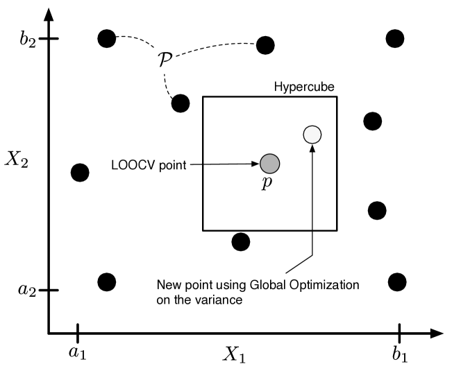
Figure 2: Sketch of a Hypercube of size $[a_{i},b_{i}]^{2}$. The grey dot is the LOO point $p$, the black dots are the surrounding points $\mathcal{P}$ and the white dot is the new point to evaluate.

The hypercube is defined by the cartesian product of the intervals of the $n$ parameters i.e. $[a_{i},b_{i}]^{n}$. The constrained optimization problem can hence be written as:

$$\left\{\begin{array}[]{rc}\max&\parallel(\mathbf{b}-\mathbf{a})\parallel_{2}\\ \mathcal{P}&\notin[a_{i},b_{i}]^{n}\\ p&\in[a_{i},b_{i}]^{n}\end{array}\right..$$ (24)

A maximum cube-volume aspect ratio ³⁴ is also defined in order to preserve the locality. This gives the new constrain

$$C:\sqrt[n]{\frac{\max(\mathbf{b}-\mathbf{a})}{\displaystyle\prod_{i=1}^{n}\max(b_{i}-a_{i})}}<\epsilon,$$ (25)

with $\epsilon=1.5$, set arbitrarily to prevent too elongated hypercubes. The global optimum is found using a two-step strategy: first, a discrete optimization using $\mathcal{P}$ gives an initial solution; second a basin-hopping algorithm ³³ finds the optimum coordinates of the hypercube. In case of the LOO-Sobol’ method, the hypercube is truncated using the total order Sobol’ indices.

4 Results

The benefits and mechanisms of the methods are first evaluated on complex analytical functions. The chosen functions are defined in Section 4.1. Then, the treatment of the parameter space’s boundary is presented in Section 4.2. Taking into account this issue, the analytical functions are tested in Section 4.3. Finally, the methods are evaluated on a realistic application in Section 4.4 with the LES of the LS89 test case ¹⁶.

4.1 Analytical functions

In order to test the new resampling methods, three analytical functions—see Table 1—with increasing numbers of input dimensions are presented, namely: (i) Rosenbrock ; (ii) Ishigami ; and (iii) g-function ^{35, 36, 7}. They all are widely used because they are nonlinear and nonmonotonic. Note that, similar results were obtained on other functions.

Function	Hypercube	Definition
Rosenbrock	$[-2.048,2.048]^{2}$	$f(X_{1},X_{2})=\sum_{i=1}^{d-1}[100(x_{i+1}-x_{i}^{2})^{2}+(x_{i}-1)^{2}].$
Ishigami	$[-\pi,\pi]^{3}$	$f(X_{1},X_{2},X_{3})=\sin X_{1}+7\sin^{2}X_{2}+0.1X_{3}^{4}\sin X_{1}.$
g-function	$[0,1]^{4}$	$f(X_{1},X_{2},X_{3},X_{4})=\prod_{i=1}^{4}\frac{\lvert 4X_{i}-2\rvert+a_{i}}{1+a_{i}},\quad a_{i}=i.$

Table 1: Analytical functions considered sorted by increasing number of input parameters.

4.2 Restriction of the DoE

The first step when constructing a model is to define the DoE. This is done by defining the range of each input parameter, the boundaries that describe a hypercube. Then, using a low discrepancy sequence as described in Section 3.1, an initial pool of snapshots is computed within the hypercube. However, when constructing a model based on Gaussian Process regression, the error is important at the boundaries of the DoE due to the lack of information. The model is thus not able to extrapolate accurately at these locations. If using the variance technique as it is, the algorithm tends to add points around the corners and only after it considers other parts of the domain. When dealing with a low dimensional case—fewer than three parameters as with the Michalewicz function which uses two input parameters, see Fig. 3—, a few iterations are "wasted" in the process.

Figure 3: Michalewicz function: dots represent the initial sample of 50 points and diamonds represent the 20 resampled points. The function was evaluated on the hypercube $[1,\pi]^{2}$

When increasing the number of parameters, there is a larger number of boundaries to cover. This has been confirmed on the Ishigami function (3 input parameters) for which the reported $Q_{2}$ values are even worse. As shown in Table 2, the optimization process is being over constrained in these regions and the global predictions are degraded. To obtain this Table, the initial sample was increased using a constant number of resampling points (10 points) and the error was measured using a uniform distribution on the domain, confirming the importance of the boundary treatment.

Initial sample	Total size	$Q_{2}$
30	40	0.05
35	45	-0.02
40	50	-0.13
45	55	-0.19
50	60	-0.04
55	65	0.43
60	70	0.51
65	75	0.87
70	80	0.54
75	85	0.86

Table 2: Error $Q_{2}$ on the Ishigami function of the size of the initial sample using a variance strategy with 10 points.

The possibility to widen the space by a delta space has been evaluated to address this question. The objective is to condition the predictor around the boundaries by adding information outside the domain of interest. A Halton sequence has been used to generate a sample of size $N_{s}=80$ from the space

$$N_{i}\sim\mathcal{U}(20,80)\quad\Delta_{space}\sim\mathcal{U}(0,20\%),$$ (26)

with $N_{i}$ the number of initial snapshots and $\Delta_{space}$ the widening factor, the outer delta space. For each case $N_{i}$, it is only the proportion of initial sample over the number of resample point that varies. (See Fig. 4). A fixed budget of $N_{b}=80$ snapshots was considered. Then, the number of resampling points is equal to $N_{rs}=N_{b}-N_{i}$. The strategy used here was the $\sigma$ model (see Section 3.1). After the resampling phase has been completed, the quality $Q_{2}$ of the model is computed. Applied to the Ishigami function, $N_{s}$ simulations each performing $N_{b}$ evaluations have been used to construct the response surface. These results were compared to a case without resampling: $N_{i}=N_{S}=80$. The resulting predictivity quality being $Q_{2}\simeq 0.8$.

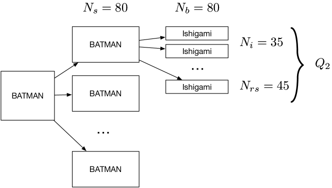
Figure 4: Example showing a computation of $Q_{2}$ with $N_{i}=35,N_{rs}=45$.

As shown in Fig. 5, there is no benefit of adding points outside the domain. Aside from the uniform distributions usually employed on this function, a standard arcsine distribution was also tested to assess the quality around boundaries but no enhancement was observed. When the delta space is increased, there is a loss of quality due to the presence of points in non-interesting regions.

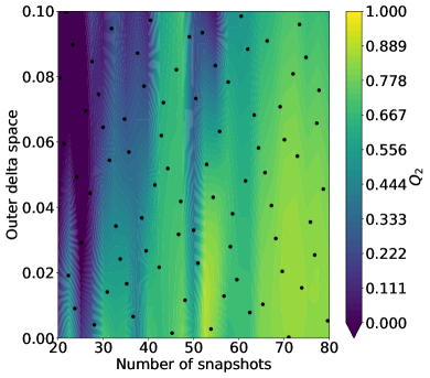
(a) Uniform distribution

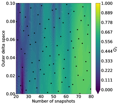
(b) Arcsine distribution

Figure 5: Response surface of $Q_{2}$ function of the initial sample and the outer delta space. Dots represent the simulations.

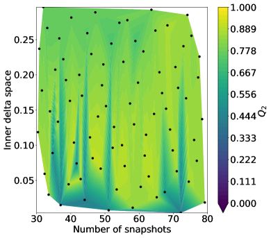
(a) Uniform distribution

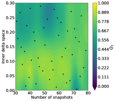
(b) Arcsine distribution

Figure 6: Response surface of $Q_{2}$ function of the initial sample and the inner delta space. Dots represent the simulations.

Complementarily to this analysis using an outer delta space, an inner delta space factor has also been considered. The same methodology was used. Results are shown in Fig. 6. On the uniform case, the model was not correctly computed due to high discontinuities caused by the  0% inner delta space cases. In ³⁷, optimal design that tends to put more points near the boundaries were shown to be more effective. Our results are coherent with their findings as we observed an improvement of the quality when using a low inner delta space. Indeed, a small value of the parameter limits the trend to add points close to the boundaries.

This work has shown that setting an inner delta space comprised between 5 and 10% is required to ensure the robustness of the model construction. Based on this observation, in the following the inner delta space is set to an arbitrary value of 8%.

4.3 Application on analytical functions

The operating mechanism and catches of the method can be visualized on the Rosenbrock function—see Fig. 7. Starting from the $\sigma$ method: points are first added close to the top boundary despite the inner delta space parameter. However, the lack of surrounding points made this choice fairly legitimate. Other points seem to be located in interesting regions—where there is a gradient and no points. It can be seen as a low discrepancy sequence, which made its use relevant for studying the delta space impact in Section 4.2. On the other hand, the LOO-$\sigma$ method does not seem to exhibit a boundary preference. But, on the bottom left-hand corner, there is an accumulation of points. Indeed, this method relies on the location of the most sensitive point. Considering the surroundings of a strong extremum—as it is the case here—, the method tends to add points first in this zone preventing further exploration of the domain and, in this case, totally misses the second extremum. Lastly, the LOO-Sobol’ method seems more balanced. Points have been added preferentially on the $X_{1}$ parameter axis, as it is slightly the most influent parameter ($S_{T_{X_{1}}}\simeq 0.7$).

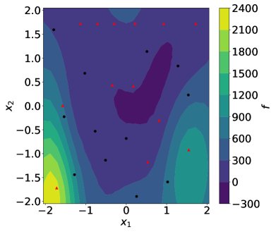
(a) $\sigma$: $Q_{2}=0.75$

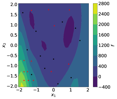
(b) LOO-$\sigma$: $Q_{2}=0.68$

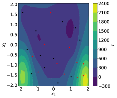
(c) LOO-Sobol’: $Q_{2}=0.86$

Figure 7: Response surface of the Rosenbrock function. In each case, the initial learning sample is composed of 12 simulations and there are 13 resampling points—respectively represented in dots and diamonds.

A convergence study has also been performed. With a fixed total number of simulations, the size of the initial learning sample was changed to evaluate the impact of the ratio of the initial sampling over the total number of samples on the quality of the model. As in Section 4.2, a Halton sequence was used. The respective parameters are reported in Table 3. The Sobol’ indices for the Ishigami function are found in ³⁸, while for the other functions, a deterministic sample of $\numprint{100000}$ evaluations was used.

Function	Sample Budget	$Q_{2}$	Total order Sobol’ indices
Rosenbrock 2-D	25	0.82	[0.71, 0.50]
Ishigami 3-D	80	0.85	[0.557, 0.443, 0.244]
g-function 4-D	65	0.66	[ 0.61, 0.29, 0.16, 0.09]

Table 3: Reference $Q_{2}$ and Total order Sobol’ indices at a fixed budget using a Halton sequence for the analytical functions.

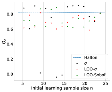
(a) Rosenbrock

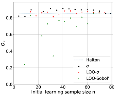
(b) Ishigami

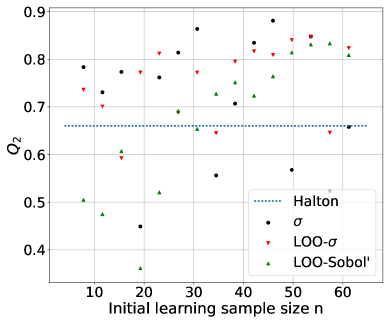
(c) g-function

Figure 8: Convergence of $Q_{2}$ of the different methods on each function by varying the initial learning sample size with a fixed budget.

Results are shown in Fig. 8. The $\sigma$ method appears to be one of the most, in some cases the most, effective method but it also exhibits more variability. Increasing dimensionality seems only to improve slightly this behaviour. There are multiple explanations to this phenomenon. The method relies on the use of an inference about the variance of the model. Starting from a given sample, if the fitting process does not converge, the prediction of the variance will be far from correct leading to a wrong resampling. Of course, there is a chance for this new point location to be relevant, still this can lead to an even worse model or an overfitting where the model is too closely linked to the outputs, so the model has memorized only the feature but not learned the underlining correlation between the data. Lastly, looking at Fig. 9, even if the points look well distributed over the parameter space, the pGP model is absolutely wrong. The Gaussian Process reconstruction failed to recover the response surface of the function whereas a Radial Basis Function Networks model successfully did it.

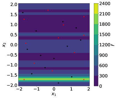
(a) Gaussian Process: $Q_{2}=0$

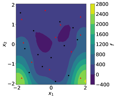
(b) RBF: $Q_{2}=0.83$

Figure 9: Response surface of the Rosenbrock function. Comparison between two models. The initial sample is composed of 13 simulations and 12 resampling points—respectively represented in dots and diamonds.

The other two methods share the $\sigma$ strategy, but the variability is conditioned by the LOO point. Indeed, the former only uses inference about the predictive variance whereas LOO’s methods take into account the observed quality of the model. LOO-Sobol’ is even more stable especially when the contribution of the parameters to the QoI is not even. The quality evolves quasi-linearly with the initial sample size. This is due to the initial guess on the indices. The closer the indices are converged, the better the sizing of the hypercube used by the $\sigma$ strategy. Indeed, some dimension of the hypercube could be neglected due to the indices. In the Rosenbrock case the method behaves like LOO-$\sigma$, the importance factors are close enough so that this collapse of dimension does not occur. On the other hand, with the g-function, the total order Sobol’ indice of the last input parameter is so small that the algorithm tends not to take into account this dimension.

For each function, as the initial sample gets close to the budget, the expected improvement is reduced. This is clear with the Ishigami function. When the initial sample is too small, the model is so poor that the points are not added efficiently. On the contrary, if we add an insufficient number of points, the impact is close to none but still there is an improvement. From the other cases, the effect of the ratio of the initial learning sample size over the total budget is not so clear. In 2-D the impact is null and after that, a ratio $>0.5$ seems appropriate.

Thus, setting aside the possible non-fitting of the data, improving the quality of the surrogate model by resampling the parameter space appears to be guaranteed in high dimensional cases and using no more than half of the budget.

4.4 LS89 case

4.4.1 Case description

The LS89 case is a blade cascade designed and tested experimentally at the Von Karman Institute for Fluid Dynamics (VKI) ¹⁶. The linear cascade consists of five high-pressure turbine vanes although only the center vane is studied. The vane is a 2D extruded profile unlike most industrial vanes that are much more complex geometrically. It however remains of great interest because the operating points are representative of values found in real engines today. This test case represents one of the largest turbomachinery databases available for the validation of CFD models in complex geometries.

A large variety of operating points have been successfully simulated until now. Low levels of turbulence injection ($<1$%) do not represent an issue for most solvers ^{39, 40} using either Reynolds-Averaged Navier Stokes (RANS) or Large Eddy Simulation (LES). Higher levels of turbulence have also been studied successfully ⁴¹ but difficulties arise for higher Reynolds numbers and larger outlet Mach numbers. Simulations are not able to correctly predict experimentally obtained profiles, notably the heat transfer field which is of great importance for the blade life-cycle.

The operating point addressed in this document, selected from Arts ¹⁶, is the MUR235, a very rich case in terms of physics that presents the above mentioned challenges (high Reynolds and outlet Mach numbers). Figure 10 highlights the main physical interactions in such a flow. One of the most notable features is the presence of a shock wave on the suction side of the blade. This shock wave interacts with a transitional boundary layer due to the highly curved flow, a potential source of instabilities in the boundary layer which in turn determines the wake downstream. This wake issues acoustic waves that impact the neighbour blade affecting the stability of the boundary layer. Also, there is a high level of free-stream turbulence that undergoes stretching around the leading edge of the blade which modifies the position of the boundary layer transition on the suction side ⁴².

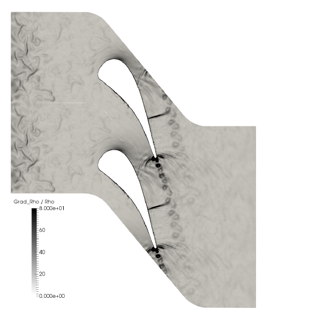
Figure 10: $\frac{\nabla\rho}{\rho}\;(m^{-1})$ with $Tu=30\%$.

In the original experiments ¹⁶, an increase in heat transfer is observed on the suction side of the blade when a high turbulence intensity level at the inlet ($\sim 6$%) as well as a large Reynolds number at the outlet ($>\numprint{1e6}$) are present. The simulations recover the shock wave that triggers an abrupt transition of the boundary layer, but turbulent spots may be found upstream of this position that can contribute to the overall heat transfer. These spots can be explained due to perturbations in the free-stream turbulence $Tu$ that are capable of trespassing the sheltering effect of the shear layer and thereby increase the heat transfer. Turbulence values upstream of the blade are thus of upmost importance.

The original experiments give only the turbulence intensity level at an upstream distance from the vane, which is insufficient to characterize the turbulent flow at this location. Recent studies on the same test bench have measured the integral length scale for the same intensity level ⁴³. In spite of this newly available information, simulations are not capable of recovering an important part of the heat flux on the suction side even when taking the correct length scale ⁴⁴. Uncertainties concerning the measured values in the experiments, that serve as boundary conditions in the simulation, appear as a path to be explored.

Apart from the turbulence intensity and the length scale, the angle of attack $\alpha$ of the incoming flow can also be seen as an uncertain parameter. There is no information related to this parameter in the experimental campaigns. In Fig. 11, the effect of $\alpha$ was numerically investigated with respect to $Tu$ by studying the heat transfer coefficient response—hereafter defined as the QoI. Due to the computational effort required to modify and simulate correctly a case with a modified integral length scale versus a modification of $\alpha$, this parameter was not taken into account. Increasing $Tu$ or $\alpha$ causes an increase of the QoI and $Tu$ seems to have a larger impact than $\alpha$. A deeper analysis would require more computations to obtain: (i) a correct response of the influence of these parameters on the QoI ; (ii) the contribution of each parameter ; and (iii) the probability density function of the QoI by propagating the uncertainties. Thus, the parameter space for this study was defined as

$$Tu\in[0,30\%]\quad\alpha\in[-5,5\mathrm{\SIUnitSymbolDegree}].$$ (27)

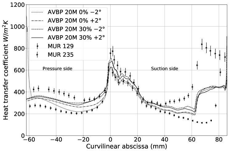
Figure 11: Heat transfer coefficient variation compared to experimental data of MUR129 ($Tu=1\%,\alpha=0\mathrm{\SIUnitSymbolDegree}$) and MUR235 ($Tu=6\%,\alpha=0\mathrm{\SIUnitSymbolDegree}$).

4.4.2 Numerical setup

The simulations have been performed using AVBP ⁴⁵, a validated CFD LES solver co-developed by CERFACS and IFP-EN. This parallel code solves the three-dimensional compressible Navier-Stokes equations for both steady and unsteady reacting flows. The code is capable of handling hybrid unstructured meshes and allows to address complex geometries. High-order numerical schemes based on the Taylor-Galerkin (TTG) family are used ⁴⁶.

The simulations were performed on a 20 million cells mesh. Five layers of prisms in the near-wall region are present allowing a higher aspect ratio. The mean $\overline{y^{+}}$ has a value of $\simeq 6.62$ which limits the physical time step to $\numprint{1.94e-8}\text{\,}\mathrm{s}$. In this context, a wall-resolved computation using the WALE ⁴⁷ model is used to take into account the proper turbulence scaling in the near-wall region. To gather enough statistics, a simulation time of $\sim\numprint{4.1}\text{\,}\mathrm{ms}$ was performed. This lead to a CPU cost, for a single computation, of $\sim 7500$ hours lasting $\sim 5$ hours on a cluster of 1440 cores.

The resolution of the mesh and the LES quality must be guaranteed to be sufficient to capture the complex physics encountered. Indeed, the interaction between the free-stream turbulence and the boundary layer requires to carefully mesh the near-wall region. It is reasonable then to compare the profiles of heat transfer obtained using the mesh for this UQ study, from here on denoted as M0, to two finer meshes M1 and M2, see  Fig. 12. The corresponding spatial distributions of ${y^{+}}$ are shown in Fig. 13 for the three meshes.

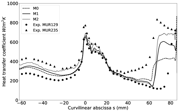
Figure 12: Heat transfer coefficient between various meshes using MUR235 setup ($Tu=6\%,\alpha=0\mathrm{\SIUnitSymbolDegree}$).

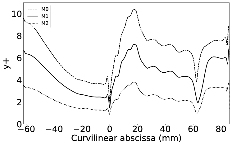
Figure 13: Refinement over blade surface measured using non-dimensional $y^{+}$ parameter for MUR235 operating point ($Tu=6\%,\alpha=0\mathrm{\SIUnitSymbolDegree}$).

The heat transfer coefficient is seen to be different on the pressure side for the finest mesh (M2). However, on the suction side the coarser mesh (M0) leads to approximately the same results as the finest mesh (M2). This suggests that the value of $y^{+}$ does not have a first order effect on the heat transfer coefficient for the meshes considered. The sensitivity to other effects such as turbulence intensity and angle of attack may thus be sought. Additionally, it can be noted that the shock wave on the suction side is located at approximately the same position for all meshes. This implies that the upstream boundary layer is similar in all cases although the heat transfer coefficient across the shock wave is affected by the mesh refinement.

4.4.3 Uncertainty Quantification results

This section presents the comparison between the different resampling methods on this complex case. In the following, an existing sample comprised of 16 simulations is used to generate a Sobol’ low-discrepancy sequence. As seen in Section 3.1, the quality of Sobol’ sequence is similar to Halton’s in low dimensional cases. Using this initial set of simulations, the sequence has been continued adding 4 points to give a total of 20 simulations. Then using the same initial sample, the previous set is compared to the use of the $\sigma$ method and the LOO-Sobol’ method. The LOO-$\sigma$ method gives similar results compared to LOO-Sobol’ method. It is not tested on this case. Quality results evaluated by LOO as described in Section 2.3 are shown in Table 4.

Method	Number of Simulations	$\hat{Q}_{2}$
Sobol’	16	0.638
Sobol’	20	0.821
$\sigma$	20	0.688
LOO-Sobol’	20	0.856

Table 4: Estimated $Q_{2}$ function of the resampling method compared to an initial sample of 16 simulations.

As demonstrated in Section 4.1, there is no guarantee that the quality of the model improves when using a refinement strategy other than continuing the low discrepancy sequence, given a low-dimensional case. The $\sigma$ method was only able to improve a little the quality of the initial design. This improvement was inferior to the simple continuation of the sequence. However, we observed an improved quality using the LOO-Sobol’ method. The importance factors’ difference between the two input parameters make it feasible to improve further the quality of the model—see Fig. 17.

The response surfaces of the models are plotted in Fig. 14. The heat transfer coefficient has been integrated over the chord line to obtain this visualization. The first thing to notice is the correct distribution of sample points within the parameter space ensuring that most of the effects are captured. The predictions obtained using the models are then found to be in agreement with the observations made previously. The heat transfer coefficient increases with the turbulence intensity and is fairly stable regarding the angle of the incoming flow. The models are said to be additive with respect to the turbulence intensity. Contrary to the Sobol’ sequence, the LOO-Sobol’ method detected that the model was sensitive to low values of turbulence intensity. It is this physical information that helped improve the predictivity quality. In the following, the model constructed using the LOO-Sobol’ method is used.

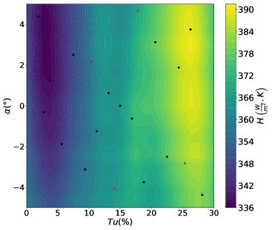
(a) Sobol’ sequence

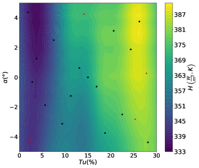
(b) $\sigma$ method

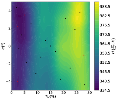
(c) LOO-Sobol’ method

Figure 14: Heat Transfer coefficient response surface. DoE is initially composed of 16 simulations sampled with Sobol’ sequence. Dots represent the initial LES simulations and diamonds represent the resampled points.

Without making any assumption on the uncertainties, the Probability Density Functions (PDF) of the input parameters are both defined using uniform distributions over the parameter space

$$Tu\sim\mathcal{U}(0,30\%)\quad\alpha\sim\mathcal{U}(-5,5\mathrm{\SIUnitSymbolDegree}).$$ (28)

Using these PDFs, uncertainties are propagated by $\numprint{5000}$ predictions of the heat transfer coefficient along the blade. Then the QoI’s PDF is reconstructed using a kernel smoothing procedure ^{48, 49}. Figure 15 reveals the expected concerning the propagation of such uncertainties to the heat transfer coefficient. As the two input distributions are uniform and the model is additive, the mean is centred between the extrema. From the experiments—see Fig. 11—the envelope of the heat transfer coefficient is correctly captured except after the shock region. Indeed, from past experiences, capturing this region requires a value of $y^{+}\sim 1-2$ ⁵⁰.

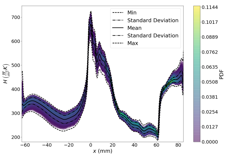
Figure 15: Probability Density Function and moments of the heat transfer coefficient along the chord line of the blade.

Finally, the Sobol’ indices have been estimated using $\numprint{200000}$ predictions. As the response surface suggested, the heat transfer coefficient is mainly affected by the variation of the turbulence intensity. The spatial evolution of the indices in Fig. 16, shows a spatial dependency. On the pressure side, the inflow angle has a higher influence as its contribution rises to become the most important parameter at the trailing edge. On the suction side, the turbulence intensity contribution is stable until the shock region. Reaching the trailing edge, the angle contribution increases. Finally, aggregated indices are reported in Fig. 17. These indices confirm that the turbulence intensity is the most important parameter compared to the inflow angle when studying the heat transfer coefficient and for the range of angle variations retained. The turbulence intensity contributes to 70% of the total variance of the QoI whereas the inflow angle contributes to 30%. This behaviour was expected as downstream the shock, the incoming level of turbulence has little impact. The computation of the second order indices are not presented here because their values are negligible in comparison to the first order indices. This is in agreement with the small differences observed between the first and total order indices. There are no joint effects between the two parameters.

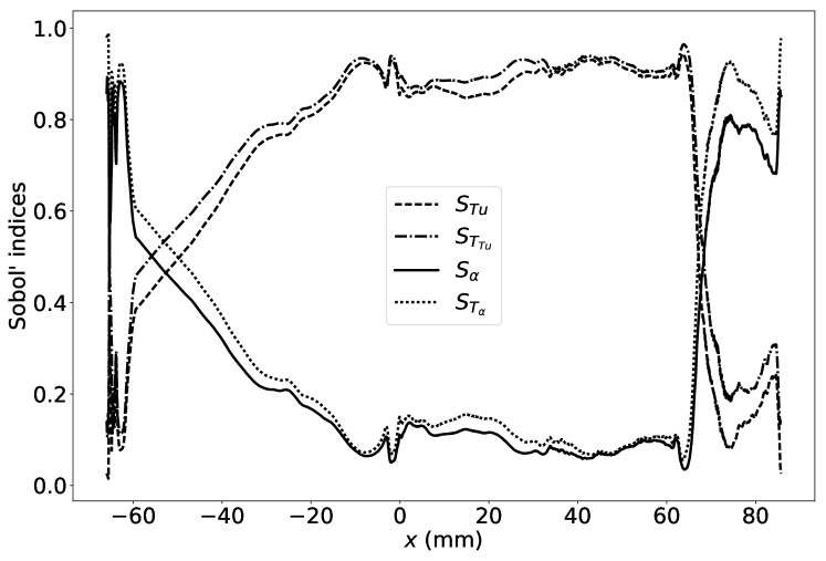
Figure 16: First order and total order Sobol’ indices along the chord line.

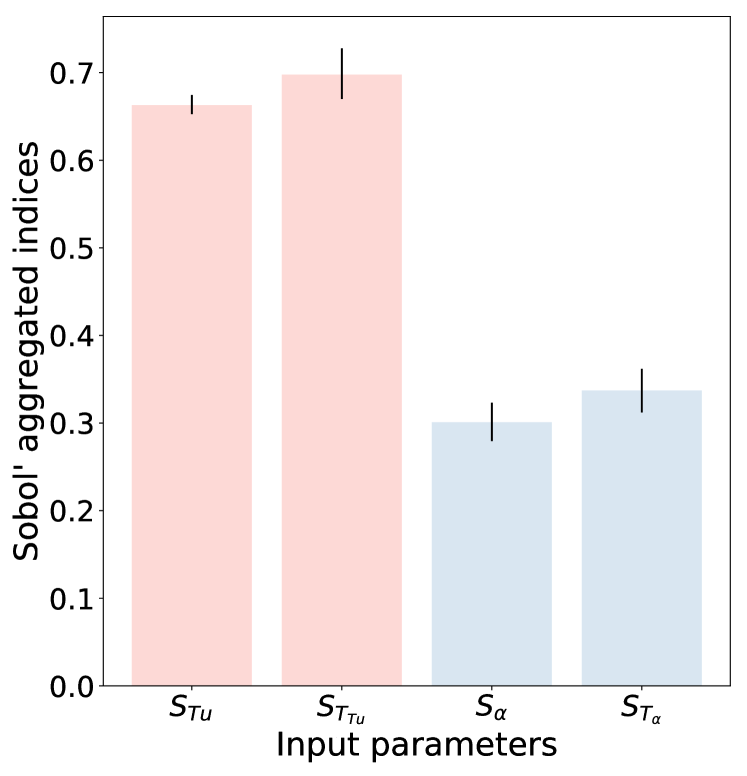
Figure 17: Aggregated Sobol’ indices of the input parameters with their asymptotic confidence intervals.

5 Conclusions

Two new methods have been introduced in this work for resampling the parameter space in order to improve the predictivity coefficient of a surrogate model: namely LOO-$\sigma$ and LOO-Sobol’ methods. These methods do not only take advantage of the capability of Gaussian Process models to infer a prediction variance, but they use information about the observed quality of the model. It was shown that an improvement of the quality of the model is guaranteed in high dimensional cases. Compared to a resampling method based on the predicted variance only, the proposed methods behaviour appears to be more stable and reliable. We also found that the ratio of the initial learning sample space over the total budget of function evaluation should remain greater than $\numprint{0.5}$. Which is to say that no more than half of the budget should be allocated to resampling the parameter space. In any case, the initial quality of the model should be reasonable when considering these techniques.

A first Uncertainty Quantification LES study of the LS89 is presented. The parameter space was comprised of the turbulence intensity and the inflow angle. In order to increase the quality of the surrogate model, the LOO-Sobol’ method was used to refine the parameter space. We showed that it performed better than continuing the sampling sequence. Apart from an analysis of the variance, the model was used to propagate uncertainties. This study reveals that although the turbulence intensity is the main factor impacting the heat transfer coefficient, there is spatial evolution of its contribution along the blade.

In terms of conclusions, by taking into account the physics in this process, the proposed methods will help build better models at lower costs. This will allow also Uncertainty Quantification of high-dimensional or expensive cases to be within reach.

References

- 1 Duchaine F, Morel T, M. Gicquel L. Y.. Computational-Fluid-Dynamics-Based Kriging Optimization Tool for Aeronautical Combustion Chambers. AIAA Journal. 2009;47(3):631–645.
- 2 Forrester Alexander I J, Keane Andy J.. Recent advances in surrogate-based optimization. Progress in Aerospace Sciences. 2009;45(1-3):50–79.
- 3 Draper David. Assessment and Propagation of Model Uncertainty. Journal of the Royal Statistical Society B. 1995;57(1):45–97.
- 4 Sacks Jerome, Welch Williams J., Mitchell Toby J., Wynn Henry P.. Design and Analysis of Computer Experiments. Statistical Science. 1989;4(4):409–423.
- 5 DeGennaro Anthony M., Rowley Clarence W., Martinelli Luigi. Uncertainty Quantification for Airfoil Icing Using Polynomial Chaos Expansions. Journal of Aircraft. 2015;52(5):1404–1411.
- 6 Masquelet Matthieu, Yann Jin, Dord Anne, et al. Uncertainty Quantification in Large Eddy Simulations of a Rich-Dome Aviation Gas Turbine. In: :1–11; 2017.
- 7 Saltelli Andrea, Ratto Marco, Andres Terry, et al. Global Sensitivity Analysis. The Primer. Chichester, UK: John Wiley & Sons, Ltd; 2007.
- 8 Martin Jay D., Simpson Timothy W.. Use of Kriging Models to Approximate Deterministic Computer Models. AIAA Journal. 2005;43(4):853–863.
- 9 Najm Habib N. Uncertainty Quantification and Polynomial Chaos Techniques in Computational Fluid Dynamics. Annual Review of Fluid Mechanics. 2009;41(1):35–52.
- 10 Rasmussen C.E., Williams C. Gaussian processes for machine learning. MIT Press; 2006.
- 11 Braconnier T., Ferrier M., Jouhaud J.-C., Montagnac M., Sagaut P.. Towards an adaptive POD/SVD surrogate model for aeronautic design. Computers & Fluids. 2011;40(1):195–209.
- 12 Margheri Luca, Sagaut Pierre. A hybrid anchored-ANOVA – POD/Kriging method for uncertainty quantification in unsteady high-fidelity CFD simulations. Journal of Computational Physics. 2016;324:137–173.
- 13 Owen N. E., Challenor P., Menon P. P., Bennani S.. Comparison of surrogate-based uncertainty quantification methods for computationally expensive simulators. 2015;:1–10.
- 14 Roy Pamphile T., El Moçayd Nabil, Ricci Sophie, et al. Comparison of Polynomial Chaos and Gaussian Process surrogates for uncertainty quantification and correlation estimation of spatially distributed open-channel steady flows. Under Final review to Stochastic Environmental Research and Risk Assessment. 2017;.
- 15 Iooss B., Boussouf L., Feuillard V., Marrel A.. Numerical studies of the metamodel fitting and validation processes. International Journal on Advances in Systems and Measurements. 2010;3(1):11–21.
- 16 Arts Tony, Lambert de Rouvroit M, Rutherford A W. Aero-Thermal Investigation of a Highly Loaded Transonic Linear Turbine Guide Vane Cascade. 174: von Karman Institute for Fluid Dynamics; 1990.
- 17 Anindya Chatterjee . An introduction to the proper orthogonal decomposition. Current Science. 2000;78(7).
- 18 Sirovich Lawrence. Turbulence and the dynamics of coherent structures part i: coherent structures. Quarterly of Applied Mathematics. 1987;XLV(3):561–571.
- 19 Krige D G, Guarascio M, Camisani-Calzolari F A. Early South African geostatistical techniques in today’s perspective. Geostatistics. 1989;1:1–19.
- 20 Marrel Amandine, Iooss Bertrand, Laurent Beatrice, Roustant Olivier. Calculations of Sobol indices for the Gaussian process metamodel. Reliability Engineering & System Safety. 2009;94(3):742 - 751.
- 21 Kohavi Ron. A Study of Cross-Validation and Bootstrap for Accuracy Estimaiton and Model Selection. In: ; 1995.
- 22 Forrester Alexander I.J., Sóbester András, Keane Andy J. Multi-fidelity optimization via surrogate modelling. Proceedings of the Royal Society A: Mathematical, Physical and Engineering Sciences. 2007;463(2088):3251–3269.
- 23 Iooss B., Saltelli A.. Introduction to Sensitivity Analysis. In: Springer International Publishing 2016 (pp. 1–20).
- 24 Ferretti Federico, Saltelli Andrea, Tarantola Stefano. Trends in sensitivity analysis practice in the last decade. Science of The Total Environment. 2016;568:666–670.
- 25 Sobol′ I.M. Sensitivity analysis for nonlinear mathematical models. Mathematical Modeling and Computational Experiment. 1993;1(4):407–414.
- 26 Marrel Amandine, Saint-Geours Nathalie, De Lozzo Matthias. Sensitivity Analysis of Spatial and/or Temporal Phenomena. In: Springer International Publishing 2015 (pp. 1–31).
- 27 Baudin Michaël, Boumhaout Khalid, Delage Thibault, Iooss Bertrand, Martinez Jean-Marc. Numerical stability of Sobol’ indices estimation formula. In: ; 2016; Réunion Island.
- 28 Cavazzuti Marco. Design of Experiments. In: Springer Berlin Heidelberg 2013 (pp. 13–42).
- 29 Fang Kai-Tai, Li R Z, Sudjianto A. Design and modeling for computer experiments. 2006.
- 30 Damblin Guillaume, Couplet Mathieu, Iooss Bertrand, Damblin Guillaume, Couplet Mathieu, Iooss Bertrand. Numerical studies of space filling designs : optimization of Latin Hypercube Samples and subprojection properties. Journal of Simulation. 2013;:276–289.
- 31 Mckay M. D., Beckman R .J., Conover W. J.. A Comparison of Three Methods for Selecting Values of Input Variables in the Analysis of Output from a Computer Code. Technometrics. 1979;21(2):239–245.
- 32 Scheidt Céline. Analyse statistique d’expériences simulées : Modélisation adaptative de réponses non-régulières par krigeage et plans d’expériences, Application à la quantification des incertitudes en ingénierie des réservoirs pétroliers. PhD thesisLouis Pasteur2006.
- 33 Wales David J., Doye Jonathan P. K.. Global Optimization by Basin-Hopping and the Lowest Energy Structures of Lennard-Jones Clusters Containing up to 110 Atoms. The Journal of Physical Chemistry A. 1997;101(28):5111–5116.
- 34 Smith Warren D., Wormald Nick. Geometric Separator Theorems and Applications. In: ; 1998.
- 35 Molga Marcin, Smutnicki Czesław. Test functions for optimization needs. 2005;(c):1–43.
- 36 Ishigami T., Homma T.. An importance quantification technique in uncertainty analysis for computer models. IEEE. 1990;:398–403.
- 37 Dette Holger, Pepelyshev Andrey. Generalized Latin Hypercube Design for Computer Experiments. Technometrics. 2010;52(4):421–429.
- 38 Marrel Amandine, Iooss Bertrand, Da Veiga Sébastien, Ribatet Mathieu. Global sensitivity analysis of stochastic computer models with joint metamodels. Statistics and Computing. 2012;22(3):833–847.
- 39 Gourdain N., Duchaine F., Collado E., Gicquel L.. Advanced Numerical Simulation Dedicated to the Prediction of Heat Transfer in a Highly Loaded Turbine Guide Vane.. In: GT2010-22793 , ed. ASME Turbo expo, ; 2010; Glasgow, UK.
- 40 Emory Michael, Iaccarino Gianluca, Ma Lynn. Uncertainty Quantification in Turbomachinery Simulations. In: :1–10; 2016.
- 41 Wheeler A.P.S., Sandberg R.D., Sandham N.D., Pichler R., Michelassi V., Laskowski G.. Direct numerical Simulations of a High Pressure Turbine Vane. In: :GT2015-43133; 2015; Montreal, Canada.
- 42 Segui L.M., Gicquel L.Y.M., Duchaine F., Laborderie J.. LES of the LS89 cascade: influence of inflow turbulence on the flow predictions. In: ; 2017.
- 43 Fontaneto F.. Aero-thermal performance of a film-cooled high pressure turbine blade/vane: a test case for numerical codes validation. PhD thesisUniversity of Bergamo2014.
- 44 Pichler R., Kopriva J., Laskowski G., Michelassi V., Sandberg R.. Highly resolved LES of a Linear HPT Vane Cascade using structured and unstructured codes. In: GT2016-57189; 2016; Seoul, South Korea.
- 45 Gicquel L.Y.M., Gourdain N., Boussuge J.-F., et al. High performance parallel computing of flows in complex geometries. Comptes Rendus Mécanique. 2011;339(2-3):104 - 124.
- 46 Quartapelle L., Selmin V.. High-order Taylor-Galerkin methods for non-linear multidimensional problems.. 1993.
- 47 Nicoud F., Ducros F.. Subgrid-scale stress modelling based on the square of the velocity gradient. Flow Turb. and Combustion. 1999;62(3):183-200.
- 48 Wand M. P., Jones M. C.. Kernel Smoothing. Boston, MA: Springer US; 1995.
- 49 Hastie Trevor, Tibshirani Robert, Friedman Jerome. The Elements of Statistical Learning Springer Series in Statistics, vol. 2: . New York, NY: Springer New York; 2009.
- 50 Segui L.M.. Multiphysics Coupled Simulations of Gas Turbines. Unpublished. PhD thesis2017.