Plastic flow and localization in an amorphous material: experimental interpretation of the fluidity

Abstract

We present a thorough study of the plastic response of a granular material progressively loaded. We study experimentally the evolution of the plastic field from a homogeneous one to an heterogeneous one and its fluctuations in term of incremental strain. We show that the plastic field can be decomposed in two components evolving on two decoupled strain increment scales. We argue that the slowly varying part of the field can be identified to the so-called fluidity field introduced recently to interpret the rheological behavior of amorphous materials. This fluidity field progressively concentrates along a macroscopic direction corresponding to the Mohr-Coulomb angle.

I Introduction

A physical description of the elementary mechanisms underlying the plasticity of amorphous materials has emerged in the past few years based on experimental evidences and numerical investigations Barrat2011 . One of the basic ingredient is the fact that at an elementary level, plasticity occurs through local plastic events implying only a few number of constituents Argon1979 ; Spaepen1977 , typically a few tens Kabla2003 ; Schall2007 ; Amon2012 . Such events are schematically represented in Figure 1(a). When such events occur, they redistribute stress Maloney2006 ; Tanguy2006 ; Tsamados2008 . This redistribution can trigger other rearrangements generating avalanches of events. An important point of this description is its universality as the stress redistribution is independent of the local interaction between the constituents. The mechanical properties that intervene in this description are the elastic properties which characterize the amorphous material on a large scale as an effective medium. The rearrangement can be treated theoretically as a small inclusion in an elastic matrix and the stress redistributed can be computed as shown by J. D. Eshelby Eshelby1957 . The coupling between the plastic events is then quadrupolar.

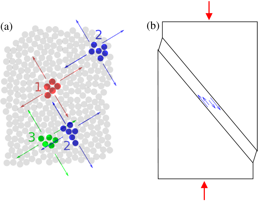
Figure 1: Schematic pictures of a plastic flow in athermal materials. (a) At a microscopic scale, a small goup of elements reorganizes and redistributes mechanical stress in the material. This initial event can trigger a cascade of other rearrangements represented schematically with other colors to indicate their order of occurence. (b) At a macrocsopic scale, the flow concentrates into a narrow zone of the material such as a shear band.

While there is now an agreement about the validity of this picture in the community, the question of how this microscopic picture builds up in a macroscopic flow is still open.

For athermal materials, an important point is to model how the flow can be self-sustained. A possible approach is at a coarse-grained level. In order to describe rheology of yield stress material, Hebraud and Lequeux Hebraud1998 introduced a local internal variable which represents the spatial and temporal density of plastic events occurring at a given time and at a given position. At a given point, this quantity evolves due to some stress relaxation, macroscopic loading and a background of mechanical noise due to plastic events occurring everywhere in this sample. The use of this internal variable, usually called fluidity, have been very fruitful to explain the rheology of yield-stress fluid. However, numerous studies evidence that local constitutive equations for the rheology are not compatible with the observations Goyon2008 . A plastic flow in a point of a material has an effect on the response of the material at some distance. A new class of nonlocal constitutive models have then been introduced Goyon2008 ; Bocquet2009 . The length characterizing the range of this interaction between events is called the cooperativity length and is supposed to depend on the distance of the local stress to the yield stress. Such a model has been adapted to granular materials and describes the stationary response of granular materials in numerous configurations Kamrin2012 ; Henann2013 .

An important feature usually observed in amorphous materials is the fact that strain localization are observed at a large scale Schall2010 . When a yield stress material is sheared homogeneously the deformation is not homogeneously allocated in the sample but is concentrated in thin parts, called shear bands, in which the strain rate is large while the other parts of the material experience small strain rate (Fig. 1(b)). A description of how those stationary shear bands emerge from microscopic elementary plastic events or from an homogeneous fluidity field is still missing. At a macroscopic point of view, to describe shear bands is to consider a stress-based failure criterion. When the local stress is larger than a threshold, called the yield stress, the material flows. In the particular case of granular materials, the failure criterion is given by the Coulomb threshold: failure occurs when the ratio of the local shear stress to the pressure is larger than $\tan\phi$ where $\phi$ is the angle of internal friction. Experimentally the internal friction angle is defined from the value of the yield stress. It may also been determined from the angle between the failure plane and the principal stress direction using a Mohr-Coulomb construction. Such a description of plasticity of shear bands has several limitations and in particular the fact that no lengthscale is introduced in the failure criterion so that the width of the shear band cannot be predicted.

In summary, the picture emerging from the literature is the following. At a microscopic scale the particles move. At a mesoscopic scale, individual plastic events may be defined, and such events are coupled by elasticity. At a macroscopic scale, the rate of such events may be theoretically represented by a variable called fluidity, which varies at the scale of the flow. Finally, macroscopic experimental observations show that strain localization occurs. Experiments or numerical simulations showing simultaneously those different behaviors are missing. We propose in this study an experiment that evidences many features of those plastic flow behaviors. For this we performed experiments on a shear flows of athermal spheres. Using an interferometric technique, we are able to follow the fluctuations of plasticity. Those fluctuations evidence some features of individual plastic events, such as the coupling of events by elasticity. If those fluctuations are averaged, a slowly varying field of deformation emerges, that may be identified with the fluidity field defined theoretically. Depending of the temporal scales at which the plasticity field is observed, different behaviors at mesoscopic and macroscopic scales may be evidenced simultaneously.

The manuscript is organized in the following way. In section II we present the experimental setup. In section III, the behavior of the correlation functions of the plasticity field is investigated. Those correlations functions can be separated into a slow and a fast component as shown in section IV. Finally, in section V, we discuss the identification of the slow component of the plastic flow to the fluidity field.

II Experimental Set-up

The experimental setup consists of a biaxial compressive test in plane strain conditions already described extensively in  LeBouil2014a . This kind of plane-strain compression is also very common in geomechanics  Viggiani2004 . The granular material (dry glass beads of diameter $d=70-110\text{\,}\mathrm{\SIUnitSymbolMicro m}$, initial volume fraction $\approx 0.60$) is placed between a preformed latex membrane ($85\times 55\times 25\text{\,}{\mathrm{mm}}^{3}$) and a glass plate. A pump produces a partial vacuum inside the membrane, creating a confining stress $-\sigma_{xx}\simeq 30\text{\,}\mathrm{kPa}$ (see Fig. 2). The sample is placed in the biaxial apparatus where displacement normal to the $xy$ plane is prevented by the front glass plate and a back metallic one, ensuring plane-strain conditions. At the bottom the sample is blocked by another metallic plate, while an upper plate is displaced vertically by a stepper motor. The stress applied at the top of the sample is then $-\sigma_{yy}=-\sigma_{xx}+F/S$, where $F$ is the force measured by a sensor fixed to the upper plate, and S the section of the sample. The velocity of the motor is $1\text{\,}\mathrm{\SIUnitSymbolMicro}\mathrm{m}\cdot\reciprocal\mathrm{s}$, leading to a deformation rate $\dot{\varepsilon}=1.2\times 10^{-5}\text{\,}\reciprocal\mathrm{s}$ (where the deformation is defined as $\varepsilon=-\varepsilon_{yy}=\delta/L$ - see inset Fig. 3). The corresponding loading curve is presented in Fig. 3(b). We work in the quasistatic regime. Note that the stress gradient due to gravity is negligible, and the value of the confining stress is too low to expect a crushing of particule. To break the symmetry when failure occurs, for instance, to study the behavior of the shear band (see nguyen2016 ), the metallic plate at the bottom of the sample can freely translate in the x-direction thanks to a roller bearing. In the following, experiments that are presented are made in this latter configuration.

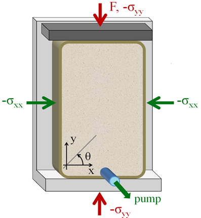
Figure 2: Schematic representation of a biaxial setup. The granular material is enclosed between a latex membrane and a glass plate (not represented here). A partial vacuum inside the sample creates a confining stress $-\sigma_{xx}=30$ kPa. At the top, a moving plate exerts a compression of the sample at fixed velocity along the $y$-axis. The back plate as well as the front glass one forbid displacement along the $z$-direction ensuring plane-strain conditions.

Deformations are observed through the front glass plate using a Diffusing Wave Spectroscopy (DWS) method already described before in  erpelding2008 ; erpelding2013 . A laser beam at $532\text{\,}\mathrm{nm}$ is expanded to illuminate the entire sample. The light undergoes multiple scattering inside the granular material and we collect the backscattered rays. The latter interfere and form a speckle pattern. The image of the front side of the sample is recorded by a $7360\times 4912$ pixels camera. Speckle images are subdivised in square zones of size $16\times 16$ pixels and compared using a correlation method explained elsewhere  erpelding2008 ; Amon2017 . For each zone the correlation between two successive images 1 and 2 is computed as follows:

$$g_{I}^{(1,2)}=\frac{\langle I_{1}I_{2}\rangle-\langle I_{1}\rangle\langle I_{2}\rangle}{\sqrt{\langle I_{1}^{2}\rangle-\langle I_{1}\rangle^{2}}\sqrt{\langle I_{2}^{2}\rangle-\langle I_{2}\rangle^{2}}}$$ (1)

where $I_{1}$ and $I_{2}$ are intensities of the pixels of two successive images and the averages $\langle.\rangle$ are done over the $16\times 16$ pixels of a zone. We obtain correlation maps where each pixel is calculated from eq. (1) and corresponds to a volume of area in the front plane $4d\times 4d$ and depth of a few $d$. Examples of such maps of correlation are given in Fig. 3(a). The normalisation used in (1) leads to values for $g_{I}$ in the interval $[0,\,1]$ (see the colorscale). The decorrelation of the backscattered light (i.e. low value of $g_{I}$) comes from relative beads motions as, for example, combinations of affine and nonaffine bead deplacements or rotation of nonspherical beads. In the following, maps of correlation are calculated between two successive images with a fixed axial deformation increment $\delta\varepsilon=3.5\times 10^{-5}$.

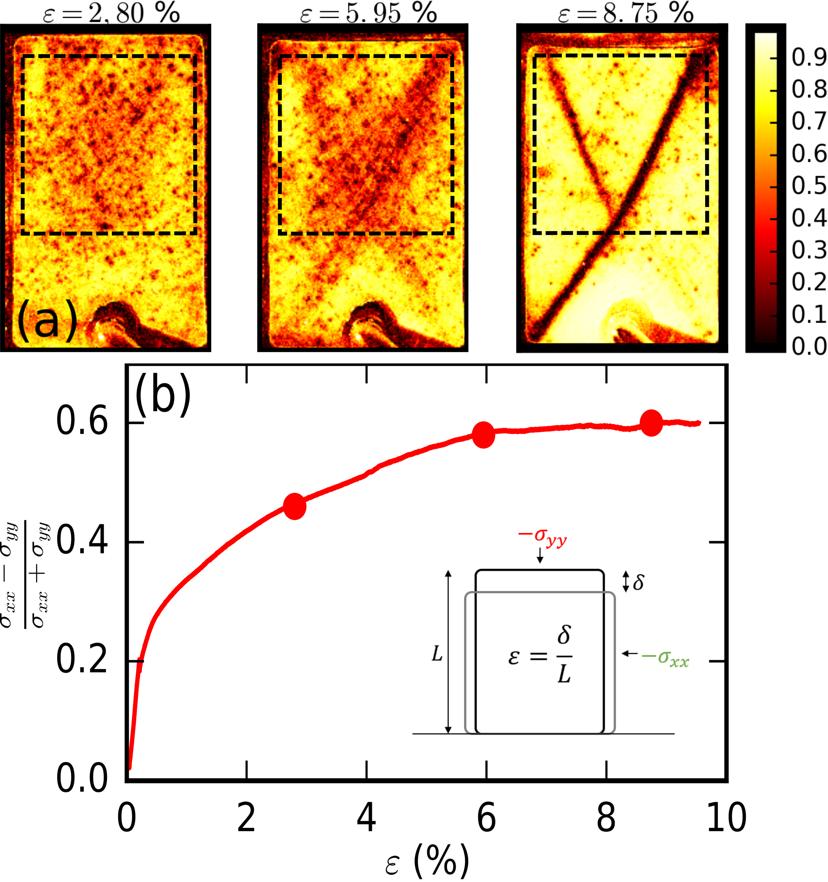
Figure 3: (a) Correlation maps $g_{I}$ for three different values of $\varepsilon$ (2.80 %; 5.95 % and 8.75 %). The region of interest used for image analysis is shown in dashed line. (b) Loading curve. Dots symbolize the positions of the three correlation maps. Inset : notations.

III Spatio-Temporal correlation functions

Observations made on the correlation maps during the loading are the same as those already presented in  LeBouil2014a ; LeBouil2014b ; nguyen2016 . In the sample, deformations are distributed inhomogeneously (see Fig. 3(a)). At the beginning of the loading, plastics events are randomly distributed throughout the sample. After a deformation of a few percent ($\varepsilon\simeq 3\,\%$) these plastic activities are organized along intermittent micro-bands until one or two permanent shear bands are established. We relate the former to avalanches of local rearrangements predicted in the microscopic descriptions of the plasticity of amorphous materials. The latter are in agreement with the Mohr-Coulomb model. In the following, we present a method to isolate each of these contributions to plasticity.

III.1 Spatio-temporal correlation function

First, we introduce a new parameter $a(\mathbf{r},\varepsilon)=1-g_{I}^{(1,2)}$ where $g_{I}^{(1,2)}$ (see (1)) is calculated on a square area of ($4d\times 4d$) at position $\mathbf{r}$. $I_{1}$ and $I_{2}$ are intensities of pixel images taken respectively at $\varepsilon_{1}=\varepsilon$ and $\varepsilon_{2}=\varepsilon+\delta\varepsilon$. Thus $a(\mathbf{r},\varepsilon)$ represents the activity at position $\mathbf{r}$ around the deformation $\varepsilon$.

We define also a spatio-temporal correlation function as follow :

$$C(\varepsilon,d\varepsilon,d\mathbf{r})=\langle a(\mathbf{r^{\prime}},\varepsilon^{\prime})\cdot a(\mathbf{r^{\prime}}+d\mathbf{r},\varepsilon^{\prime}+d\varepsilon)\rangle\\ -\langle a(\mathbf{r^{\prime}},\varepsilon^{\prime})\rangle\langle a(\mathbf{r^{\prime}}+d\mathbf{r},\varepsilon^{\prime}+d\varepsilon)\rangle$$ (2)

where $\mathbf{r^{\prime}}$ and $\mathbf{r^{\prime}}+d\mathbf{r}$ have to be in the region of interest (ROI, see Fig. 3(a)) and the deformation $\varepsilon^{\prime}$ in the interval $[\varepsilon;\varepsilon+\Delta\varepsilon]$. Keep in mind that $g_{I}^{(1,2)}$ and consequently $a(\mathbf{r},\varepsilon)$ are calculated over an increment $\delta\varepsilon=3.5\times 10^{-5}$. So there is no integration of mean displacement over $[\varepsilon\,;\,\varepsilon+\Delta\varepsilon]$. Averages are made over all pairs of pixels for which $\mathbf{r^{\prime}}$ and $\mathbf{r^{\prime}}+d\mathbf{r}$ are in the ROI and over a deformation span $\Delta\varepsilon$. In the following, the value of $\Delta\varepsilon$ is fixed at $\Delta\varepsilon=0.35\,\%$. This value is large enough to have good averages but remains small compare to the total deformation applied. Note that in all the following the deformation plays the role of time. Our experiments are in quasi-static conditions. A process which can be observed only for small deformation increments will be called a fast process in the following while a feature that lasts for large strain increments will be called a slow process.

III.2 Temporal scale of fluctuations

Throughout the loading, we can observe on the correlation maps that micro-bands are fluctuating rapidly while shear bands evolves slowly. To quantify the temporal scale of the fluctuating part, we compute temporal correlations as follow:

$$C_{T}(\varepsilon,d\varepsilon)=C(\varepsilon,d\varepsilon,d\mathbf{r}=\mathbf{0})$$ (3)

where $C_{T}$ can be interpreted as a spatial autocorrelation function giving only the temporal information.

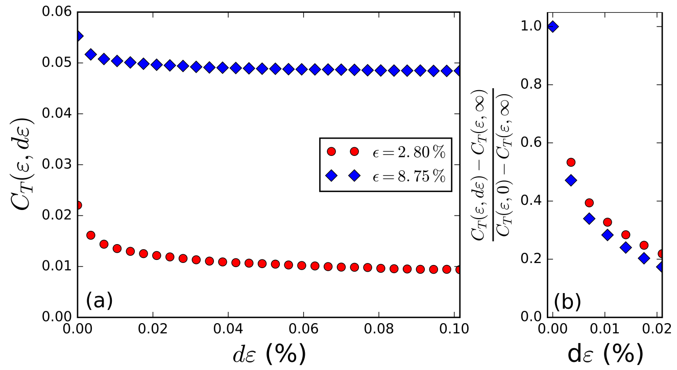
Figure 4: (a) Temporal correlation function as a function of $d\varepsilon$ at the beginning ($\varepsilon=2.80\%$) and at the end ($\varepsilon=8.75\%$) of the loading. (b) Rescaled correlation functions showing the initial drop over a characteristic gap $d\varepsilon^{*}\approx 0.01\,\%$.

Fig. 4 shows $C_{T}(\varepsilon,d\varepsilon)$ as a function of $d\varepsilon$ at two points in the loading $\varepsilon=2.80\,\%$ and $\varepsilon=8.75\,\%$. A rapid decorrelation for a gap $d\varepsilon^{*}\approx 0.01\,\%$ is initially observed, followed by a second smoother decay which tends to a non-zero finite value because of the heterogeneity of the mean field. The scale in deformation increment over which the initial drop takes place, $d\varepsilon^{*}\approx 0.01\,\%$, gives us an estimation of the temporal scale of the fluctuating part.

III.3 Separation method

The aim is to separate the two plastic phenomena throughout the loading. Our method is based on their different temporal properties. As discussed in section III.2, the fluctuating part is no longer correlated for a gap of deformation larger than $d\varepsilon^{*}$. In the case when $d\varepsilon\gg d\varepsilon^{*}$, the spatio-temporal correlation function $C(\varepsilon,d\varepsilon,d\mathbf{r})$ corresponds only to the slow part. In the following, we define the correlation function for the slow part by taking arbitrary ${d\varepsilon=\Delta\varepsilon/2=0.175\,\%\gg d\varepsilon^{*}}$ for the spatio-temporal correlation function:

$$C_{\text{slow}}(\varepsilon,d\mathbf{r})=C\left(\varepsilon,\frac{\Delta\varepsilon}{2},d\mathbf{r}\right)$$ (4)

In the same way, for $d\varepsilon\ll d\varepsilon^{*}$ the spatio-temporal correlation function $C(\varepsilon,d\varepsilon,d\mathbf{r})$ contains all the fluctuations. Thus, we define the total correlation function by taking $d\varepsilon=0$ as follows:

$$C_{\text{tot}}(\varepsilon,d\mathbf{r})=C(\varepsilon,0,d\mathbf{r})$$ (5)

Finally, the correlation function describing the fluctuating part is obtained as follows:

$$C_{\text{fast}}(\varepsilon,d\mathbf{r})=C_{\text{tot}}(\varepsilon,d\mathbf{r})-C_{\text{slow}}(\varepsilon,d\mathbf{r})$$ (6)

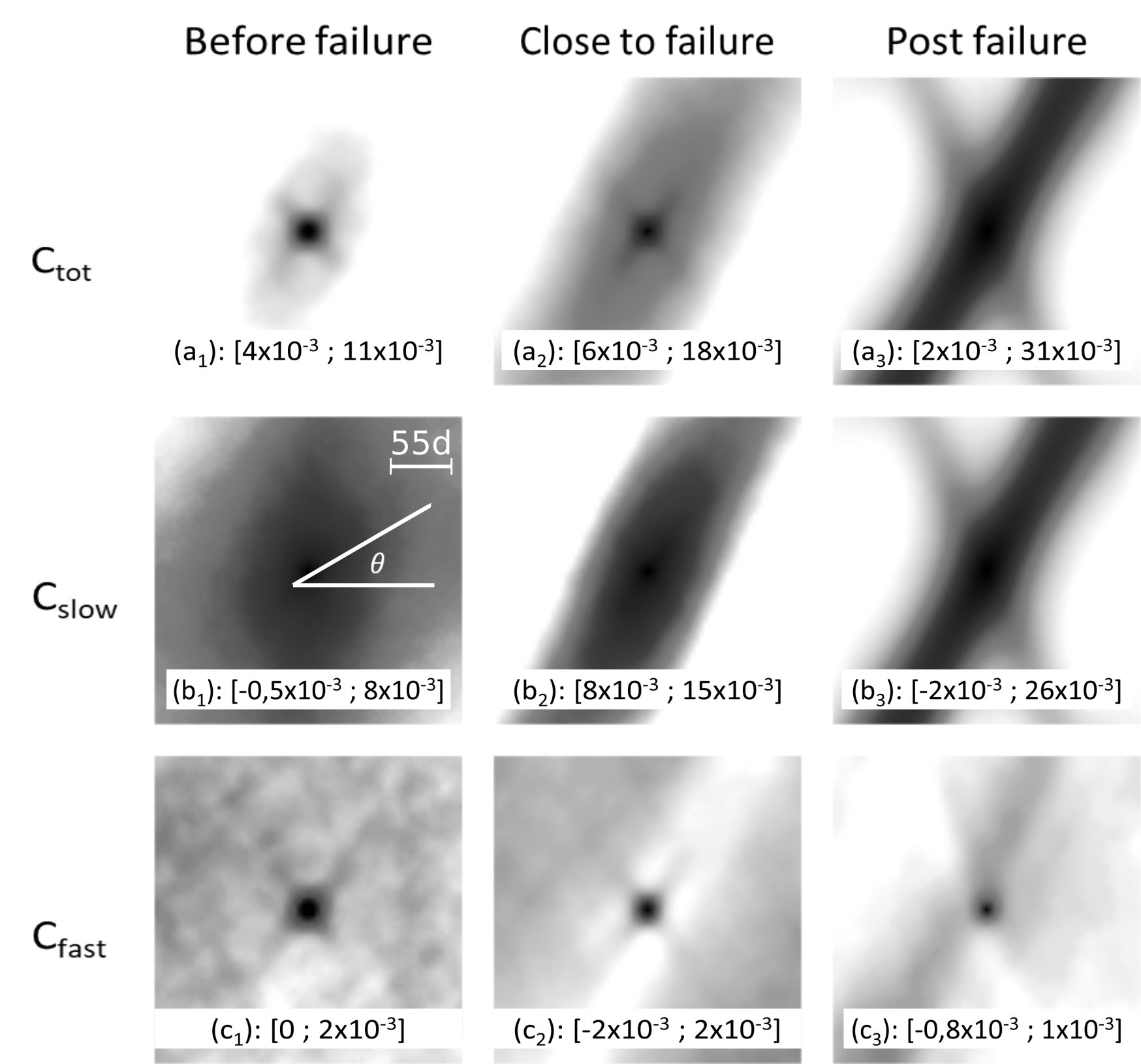
Figure 5: Spatial representation of the different parts of the correlation function for different values of the loading. All maps are centered at $d\mathbf{r}=\mathbf{0}$. The spatial scale, in unit of beads diameter, is represented in (b1). Top row ((a1), (a2) and (a3)): total correlation function $C_{\text{tot}}$; Middle row ((b1), (b2) and (b3)): slow part $C_{\text{slow}}$ of the correlation function; Bottom row ((c1), (c2) and (c3)): fast part $C_{\text{fast}}$ of the correlation function. Left column, the system is well before failure, $\varepsilon=2.80\,\%$; Middle column, it is close to the failure $\varepsilon=5.95\,\%$; Right column, after failure $\varepsilon=8.75\,\%$. Scale represented by intervals corresponds to white and black pixels respectively.

Fig. 5 shows the correlations functions $C_{\text{tot}}$, $C_{\text{slow}}$ and $C_{\text{fast}}$ defined previously. Those correlations functions are computed at different macroscopic deformation $\varepsilon=2.80\,\%$ (well before failure), $\varepsilon=5.95\,\%$ (close to failure), and $\varepsilon=8.75\,\%$ (post-failure).

IV Experimental results

IV.1 Behavior of the slow and fast parts

In this subsection, we discuss the results obtained by the calculation of the slow and fast parts of the correlation functions, and we evidence the differences of behavior between the long and the short time correlation functions.

We first discuss the correlation function near failure (middle column in Fig. 5) where the characteristic behavior is clearly visible. The total correlation function $C_{\text{tot}}$ (see Fig. 5(a2)) displays two different spatial features. Near $d{\bf r}=0$, we observe a high correlation along two directions, forming a small cross at the center of the figure. At large distance, the correlation prevails along a large inclined band spanning the full image. The fast part and the slow part of the total correlation function displays each only one of those two spatial behaviors. The fast part displays only the small cross near $d{\bf r}=0$ (Fig. 5(c2)), whereas the large inclined band belongs to the slow part (Fig. 5(b2)).

In the pre-failure stage, Fig. 5(c1) shows a fluctuating contribution at short distances, but the slow part of the correlation function (Fig. 5(b1)) remains spread on the full image and displays no structure. After failure, the slow part of the correlation function appears clearly correlated along two bands (Fig. 5(b3)), whereas the quadrupolar structure of the fluctuating part near the origin is no longer visible.

IV.2 Geometrical characterisation of the correlations.

Fig. 5 evinces that the fast and slow components of the correlation functions are both anisotropic, but with slightly different directions. We now use this observation to quantify the duality of the correlation functions with the time-scale.

For this, we need to determine the angles at which the correlation enhancement occurs. We use a projection method inspired by what has been done previously nguyen2016 . As the correlation maps are centered (see Fig. 5), we compute the mean value of the pixels intersected by a line passing through the center and with an angle $\theta$ with the $x$-axis. Next we plot these mean values as a function of the angle $\theta$ between $-\pi/2$ and $+\pi/2$. Fig. 6(a) shows the result of such projection of the fast part of the correlation $C_{\text{fast}}$ for an axial deformation $\varepsilon=5.95\,\%$. Fig. 6(b) shows the projection of the slow part of the correlation $C_{\text{slow}}$ for $\varepsilon=8.75\,\%$. From a projection profile as the ones obtained in Fig. 6, we determine the angle characterizing a response as the mean of the absolute values of the angles at which occur the maxima of the curve. Error bars are determined as the difference between the angles at which the maxima occur and the ones obtained from gaussian interpolations of the projection profile on each halves of the $[-\pi/2,\pi/2]$ interval.

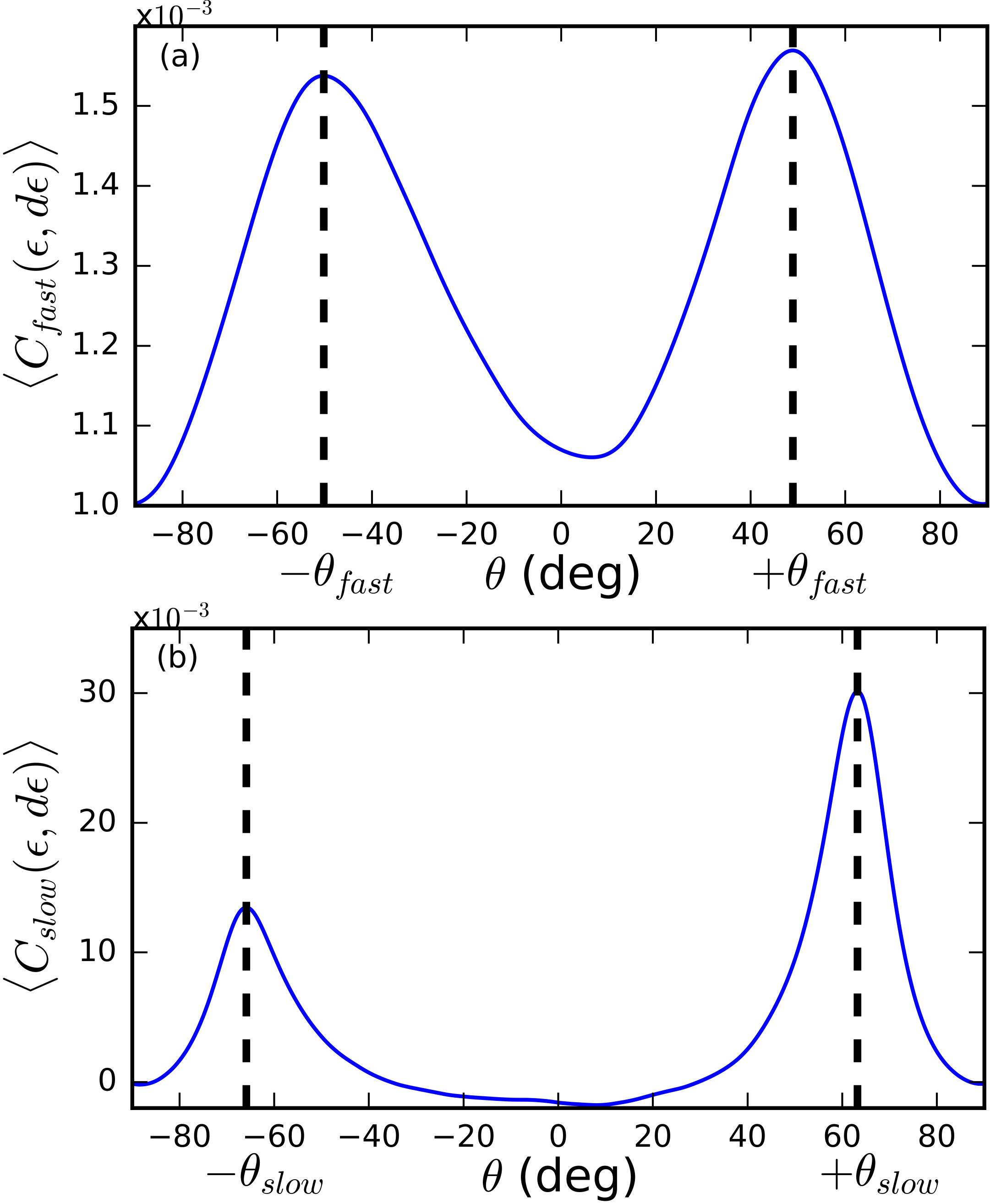
Figure 6: Angular projection of the spatial correlation functions, i.e. mean value of the pixels intersected by a line passing through the center of a spatial correlation function and making an angle $\theta$ with the $x$-axis as a function of $\theta$ for (a) $C_{\text{fast}}$ at $\varepsilon=5.95\,\%$ and (b) $C_{\text{slow}}$ at $\varepsilon=8.75\,\%$.

Fig. 7 shows the values of the angles at which the fast and the slow part of the correlation function are respectively maximals as a function of the macroscopic deformation in the $\varepsilon\in[2.45\,\%;9.80\,\%]$ range. The failure occurs for $\varepsilon\simeq 6.65\,\%$. We observe that angles at which correlation occurs are clearly different for the fluctuating and the slow parts. For a deformation in the range $\varepsilon\in[5.60\,\%;6.65\,\%]$ the coexistence of a fast and slow correlation oriented at different angles is clearly visible. Outside this range of deformation, we were not able to define two different angles simultaneously in the correlation functions.

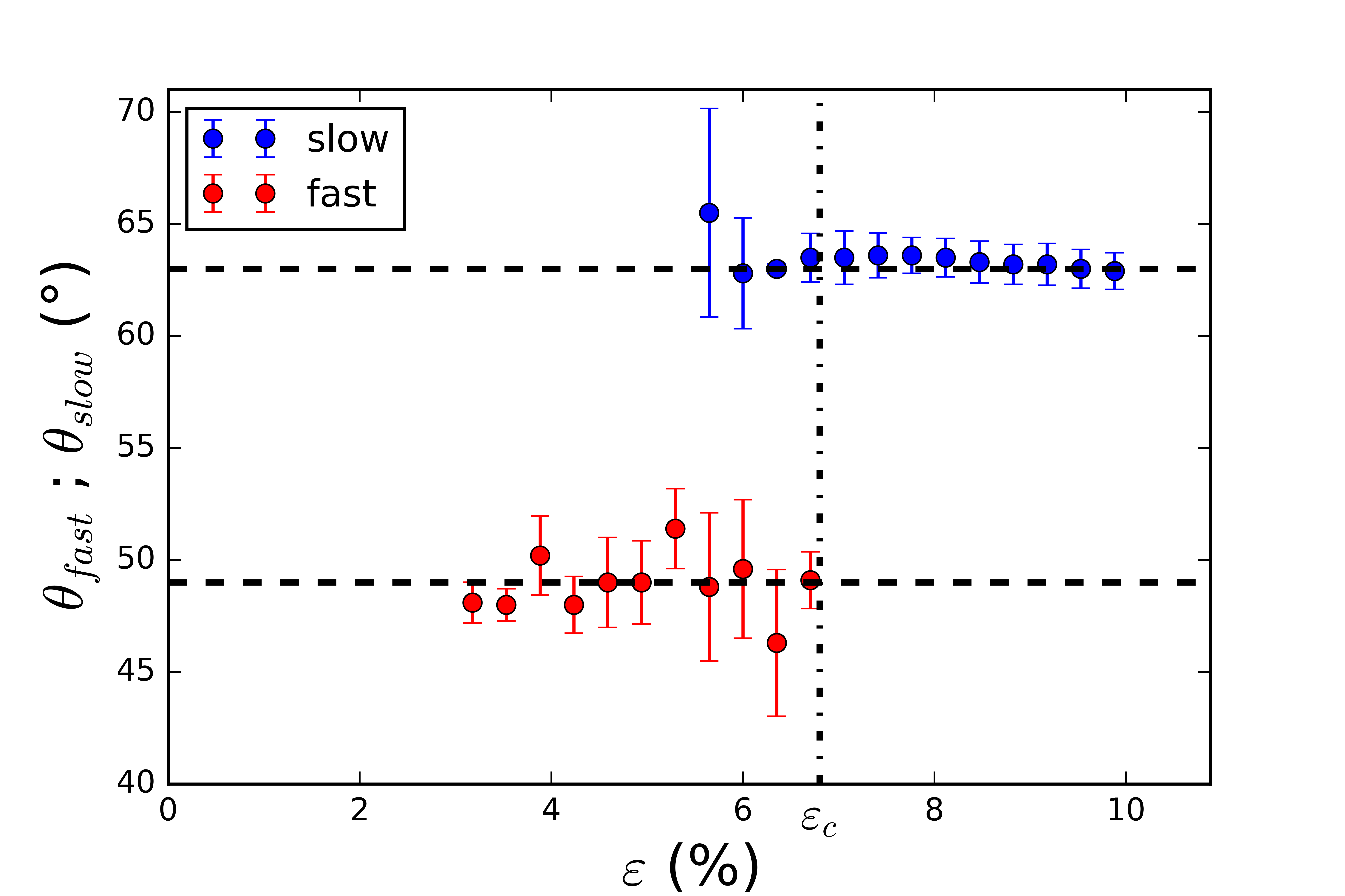
Figure 7: Angles of the fast and the slow parts of the spatial correlation function. A coexistence of two distinct directions is observed just before the failure represented by the dashed line. $\varepsilon_{c}$ stands for the critical value of the strain when the failure occurs.

V Discussion

V.1 Interpretation of geometrical angles for slow and fast correlation functions.

As it has been shown previously, we clearly observe two different angles for the correlation function. The fast part of the correlation function is quadrupolar, with an average inclination $\theta_{E}\simeq 48^{\circ}$. This orientation may be directly linked to the direction of maximum stress redistribution given by the Eshelby tensor. We can interpret the fast correlation of the plastic events as small cascades of events as represented schematically in Figure 8. Such fluctuations has also been reported in few numerical studies Kuhn1999 ; Maloney2006 .

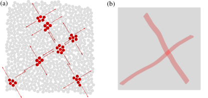
Figure 8: Schematic representation of our interpretation of the microbands as cascades of elementary events. (a) Local rearrangements coupled by elasticity. (b) Resulting deformation integrated on a larger time-scale.

The slowly varying part of the correlation function is oriented at an angle $\theta_{MC}\simeq 63^{\circ}$. This orientation may be related to the formation of a macroscopic shear band into the material. The orientation of the shear band depends on the value of internal friction ratio accordingly to a Mohr-Coulomb construction. This slow variation is related to large scale cooperative effects. It is important to note that two scales, and the two orientations coexist during the approach to failure (see Fig. 7): the fluctuations of plasticity are oriented along $\theta_{E}$ whereas the mean plasticity is oriented along $\theta_{MC}$. The two angles seem relatively constant during the loading process, and no intermediate orientations are observed, even close to failure.

V.2 Schematic interpretation of the experiment.

Figure 9 summarizes schematically our results. At the microscopic level, some grains reorganize when the applied stress is increased: this is one ”elementary event”, that is represented as a dot in Fig. 9(a1). This behavior can be observed at the very beginning of the experiment. On a larger time-scale, we observe correlated cascades of events which fluctuate rapidly Fig. 9(b1). Those micro-avalanches are inclined along a direction $\theta_{E}$ given by the Eshelby stress tensor (see Fig. 8). Increasing further the deformation field on a larger time scale, we observe a continuous field of plasticity (see Fig. 9(a3)).

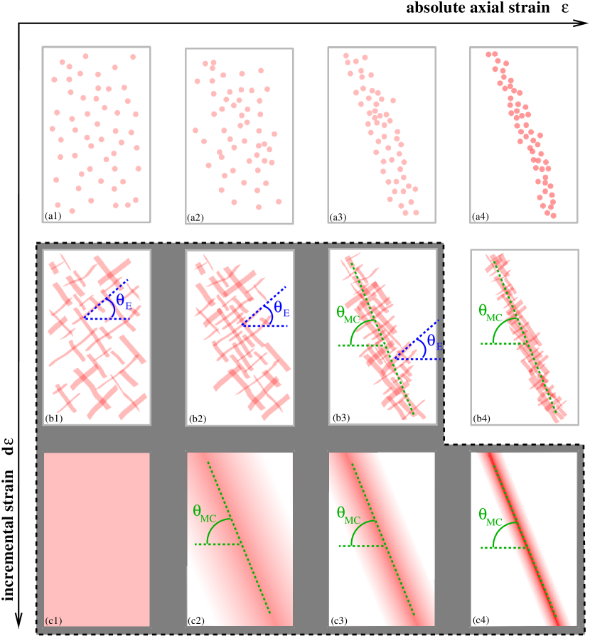
Figure 9: Schematic representation of the plastic activity at different values of the axial loading $\varepsilon$ (horizontal axis) and for different strain increments $d\varepsilon$. At an elementary level, plasticity is awaited to occur through local plastic events represented as dots on the first line. When integrating those spots on a larger strain increment, a correlated micro-strucutre emerges governed by the elastic properties of the bulk material (second line). The angle characterizing this elastic coupling, $\theta_{E}$, is given by the Eshelby kernel. On a larger strain increment this fluctuating pattern is lost and only a slowly evolving coarse-grained field remains. Shear band formation can be observed on this slow field as the emergence of an orientation $\theta_{MC}$ in the mean plastic field. The grey area displays the features actually observed experimentally. The reason why (b4) is not observed experimentally is linked to the nonlinearity in deformation of the measurement methods: the observed field saturates in the band. (a1)-(a4) are not observed because the acquisition rate is too small to reach small enough $d\varepsilon$.

At the beginning of the loading, the events repartition is roughly homogeneous at the sample scale (Fig. 9(a1)) and the corresponding mean plastic field is also homogeneous (Fig. 9(c1)). When the loading progresses, the events mainly accumulate on an active zone (Fig. 9(a2) and (a3)), and the plasticity field then becomes heterogeneous (Fig. 9(c2) and (c3)). This zone of activity is the precursor zone of the final shear band, and is inclined at an angle $\theta_{MC}$. Finally, at failure (Fig. 9(c4)), all the activity is concentrated on a narrow and stationary shear band.

V.3 Fluidity as slow part of the plastic field.

The physical interpretation of what is called fluidity is still a debated issue Bouzid2015 . The literature agrees on the fact that it corresponds to a coarse-grained field directly linked to the local plastic activity. Among the hypotheses underlying the Kinetic Elasto-Plastic model of Bocquet et al. Bocquet2009 an important point is a Boltzmann Stosszahlansatz-like hypothesis of the decoupling of the plastic-event dynamics. This means that the fluidity field is defined on a time scale large enough for the memory of the coupling between the underlying events to be lost.

We interpret the slow part of the plastic field (Fig. 9(c1) to (c4)) as the field of the so-called fluidity. Indeed, this field evolves smoothly spatially and has lost the quadrupolar symmetry of the underlying fluctuations of the plasticity. It corresponds to a coarse-grained field reflecting the local plastic activity and thus matches the theoretical definition of fluidity.

In the specific case of sheared granular materials, it has been proposed recently that a granular fluidity $g$ may be defined which is proportional to a local shear rate $\dot{\gamma}$ and which is also proportional to the velocity fluctuations $\delta v$ Zhang2017 . Experimentally (see Amon2017 for details), the speckle decorrelation is a function of the affine and the non-affine displacements of particles $\sqrt{\xi_{0}^{2}f(\varepsilon)+<\delta\xi^{2}>}$, where $\xi_{0}$ is a length of the order of the grain diameter, $f(\varepsilon)$ is a quadratic function of the affine deformation field $\varepsilon$, and $<\delta\xi^{2}>$ is the mean square non-affine displacement. The spatial scale on which the affine displacement field is defined is few bead diameters Amon2017 . For a sheared granular material, during a time $\tau$, we expect that $f(\varepsilon)\sim(\dot{\gamma}\tau)^{2}$ Amon2017 and $<\delta\xi^{2}>\sim(\delta v~{}\tau)^{2}$. It follows that $\sqrt{\xi_{0}^{2}f(\varepsilon)+<\delta\xi^{2}>}\propto g$. So our experimental probe of plastic activity seems closely related to the above-mentionned definition of the granular fluidity.

An important point in the definition of fluidity is the nature of the coarse-graining at play to obtain a smooth field. Theoretically fluidity is a variable obtained by a coarse-graining in space and time. It is unclear in the literature if this last coarse-graining is in “true” time or in strain increment. In our experiment, our technique of measurement gives intrinsically a coarse-grained measurement in space because it is based on multiple scattering of light (see erpelding2008 ; Amon2017 for a thorough discussion of the spatial resolution of the method). The measurement is also time-averaged as the acquisition rate of the camera is always much smaller than the inverse of the time of propagation of sound waves in the system. In addition to those resolution-based averages, we have studied in the present article the effect of a coarse-graining in strain increment on the observed plastic field. An important conclusion drawn from our observations is the fact that for a large enough strain increment $d\varepsilon$ the plastic field lose the memory of the “fast” correlation between the plastic events. The mean field thus obtained has its own dynamics on a slow scale. Consequently, there exists a strain increment above which a fluidity field can be defined as the slowly evolving part of the plastic field.

V.4 Inhomogeneous fluidity field and localization.

Our experiment allows to follow a fluidity field which is homogeneous at the beginning of the loading, and which condensates on a inclined band. The fact that strain localization occurs in bi- and tri-axial tests performed on granular materials is well known since many decades. However, a clear understanding of this feature is still missing Schall2007 . Some authors tried to relate strain localization with properties of the fluidity-field. In a first study, Goyon et al. Goyon2008 proposed a mechanism of formation of shear band in flows of emulsion. The authors assumed that walls that are at flow boundaries act as sources of fluidity. This fluidity then diffuses inside the sample, forming a fluid layer close to the wall. In Couette flow of granular material, fluidity increases preferentially close to the rotor because of the inhomogeneity of the stress field. In those cases, the fluidity source is localized, and the fluidity tends to spread into the sample.

In our experiment the situation is totally opposite. Fluidity accumulates on a band although the applied stress is increased homogeneously, i.e. the fluidity is initially homogeneous and finally heterogeneous. The single property that the fluidity diffuses inside the sample is not sufficient to explain this feature. Recently, Benzi and coworkers Benzi2016 have shown that shear band formation starting from an initially homogeneous fluidity in a fluidity model should be possible.

Another possible approach to understand this localization process can be to consider that there is some memory of where plasticity has already occurred. In the case of cohesive materials, the introduction of a modification of the local elastic modulus in mesoscopic models is known to lead to some localization Amitrano1999 . But the memory of previous local plastic activity is not specific to cohesive materials and can take different forms. It may described any local structural modification due to plasticity as for example a modification of the local structure or of the local packing fraction as well as the wear of some frictional contacts. In the case of shear band formation in granular materials, it is known that the packing fraction inside the flowing band takes a particular value (the so-called critical state) Andreotti2013 . The damage internal variable to take into account might then be the local packing fraction which should evolve when plastic events take place. The introduction of some memory or history-dependent effect is known to generate shear-banding in mesoscopic models Martens2012 ; Vandembroucq2011 .

V.5 Fluidity and Mohr-Coulomb theory

As mentionned in the Introduction, the Mohr-Coulomb theory gives a first order description of failure threshold and shear bands orientation for frictional materials Nedderman1992 ; Andreotti2013 . This theory introduces a frictional internal angle which is closely linked to the angle of repose for a granular material. Localisation is predicted to occur along a line which inclination is given by the internal friction. This picture of failure is very simplified but captures the prominent features observed experimentally.

In the previous parts we have shown that a shear band can be described by an inhomogeneous concentration of fluidity. Thus, it is very appealing to describe the emergence of a shear-band with a spontaneous orientation in the framework of fluidity theory. To our knowledge, in the current versions of this theory, shear bands orientation is always given by the loading geometry. It is very likely that a theory relying on a single internal variable is insufficient to predict the emergence of an angle in an homogeneous stress field. As discussed in the previous part, the introduction of another internal variable describing a form of damage might be necessary to display localization along an inclined line. This damage variable is likely to be linked to the local packing fraction. Nevertheless, the existence of a macroscopic friction in the absence of dilantancy for frictionless particles Peyneau2008 suggests that packing fraction might not be the right variable.

Very recently, a mesoscopic model using a local Mohr-Coulomb criterion and taking into account the tensorial nature of the stress redistribution have been able to reproduce macroscopic localization in the absence of a damage variable Karimi2018 as well as an orientation for avalanches different from the local coupling. Taking into account the redistributed pressure in addition to the deviatoric stress suggests also to introduce another internal variable to describe the effect of the pressure redistribution.

VI Conclusion

In this work we have discussed the nature of the spatio-temporal correlations observed in the plastic response of a granular material submitted to a biaxial test. We have detailed a procedure allowing us to separate a fluctuating component of the plastic field at small strain increments from a slowly evolving component. Those two components correspond to two different types of behaviors: the two fields have independent and coexisting characteristic orientations. We discuss the interpretation of those two behaviors in the framework of the present debated theories of plasticity and rheology of amorphous materials. We argue that the slowly varying component of the plastic field is a good candidate to be interpreted as the so-called fluidity field introduced in the last ten years to describe nonlocal effects in the flow of amorphous materials. We underline the importance of coarse-graining in strain increment in the definition of this field.

The question of the independence or correlation between the fast and slow components of the field is still open. Even if the two orientations observed are apparently unrelated it could be possible that the slow field inherits its characteristics from the fluctuations in a non trivial manner.

VII Acknowledgements

The authors thank Sean McNamara and Jérôme Weiss for many scientific discussion and acknowledge funding from Agence Nationale de la Recherche (ANR “Relfi”, ANR-16-CE30-0022).

References

- (1) J.-L. Barrat and A. Lemaitre. Heterogeneities in amorphous systems under shear in Dynamical Heterogeneities in Glasses, Colloids, and Granular Media, vol. 150, p. 264 (Oxford University Press, 2011).
- (2) A. S. Argon. Acta Metall., 27, 47 (1979).
- (3) F. Spaepen. Acta Metall., 25, 407 (1977).
- (4) A. Kabla and G. Debrégeas. Phys. Rev. Lett., 90, 258303 (2003).
- (5) P. Schall, D. A. Weitz, and F. Spaepen. Science, 318, 1895 (2007).
- (6) A. Amon, V. B. Nguyen, A. Bruand, J. Crassous, and E. Clément. Phys. Rev. Lett., 108, 135502 (2012).
- (7) C. E. Maloney and A. Lemaître. Phys. Rev. E, 74, 016118 (2006).
- (8) A. Tanguy, F. Leonforte, and J.-L. Barrat. Eur. Phys. J. E, 20, 355 (2006).
- (9) M. Tsamados, A. Tanguy, F. Léonforte, and J.-L. Barrat. Eur. Phys. J. E, 26, 283 (2008).
- (10) J. D. Eshelby. Proc. R. Soc. A, 241, 376 (1957).
- (11) P. Hébraud and F. Lequeux. Phys. Rev. Lett., 81, 2934 (1998).
- (12) J. Goyon, A. Colin, G. Ovarlez, A. Ajdari, and L. Bocquet. Nature, 454, 84 (2008).
- (13) L. Bocquet, A. Colin, and A. Ajdari. Phys. Rev. Lett., 103, 036001 (2009).
- (14) K. Kamrin and G. Koval. Phys. Rev. Lett., 108, 178301 (2012).
- (15) D. L. Henann and K. Kamrin. Proc. Natl. Acad. Sci., 110, 6730 (2013).
- (16) P. Schall and M. van Hecke. Annu. Rev. Fluid Mech., 42, 67 (2010).
- (17) A. Le Bouil, A. Amon, J.-C. Sangleboeuf, H. Orain, P. Bésuelle, G. Viggiani, P. Chasle, and J. Crassous. Granul. Matter, 16, 1 (2014).
- (18) J. Desrues and G. Viggiani. Int. J. Numer. Anal. Meth. Geomech, 28, 279-321 (2004).
- (19) T. B. Nguyen, and A. Amon. EPL, 116, 28007 (2016).
- (20) M. Erpelding, A. Amon, and J. Crassous. Phys. Rev. E, 78, 046104 (2008).
- (21) M. Erpelding, B. Dollet, A. Faisant, J. Crassous, and A. Amon. Strain, 49, 167 (2013).
- (22) A Amon, Mikhailovskaya A., and Crassous J. Rev. Sci. Instrum., 88, 051804 (2017).
- (23) A. Le Bouil, A. Amon, S. McNamara, and J. Crassous. Phys. Rev. Lett., 112, 246001 (2014).
- (24) M. R. Kuhn. Mech. Mater., 31, 407 (1999).
- (25) M. Bouzid, A. Izzet, M. Trulsson, E. Clément, P. Claudin, and B. Andreotti. Eur. Phys. J. E, 38, 125 (2015).
- (26) Q. Zhang and K. Kamrin. Phys. Rev. Lett., 116, 058001 (2017).
- (27) R. Benzi, M. Sbragaglia, M. Bernaschi, S. Succi, and F. Toschi. Soft Matter, 12, 514 (2016).
- (28) D. Amitrano, J.-R. Grasso, and D. Hantz. Geophys. Res. Lett., 26, 2109 (1999).
- (29) Granular media: between fluid and solid. B. Andreotti, Y. Forterre, and O. Pouliquen (Cambridge University Press, 2013).
- (30) K. Martens, L. Bocquet, and J.-L. Barrat. Soft Matter, 8, 4197 (2012).
- (31) D. Vandembroucq and S. Roux. Phys. Rev. B, 84, 134210 (2011).
- (32) Statics and Kinematics of Granular Materials. R. M. Nedderman (Cambridge University Press, 1992).
- (33) P.E. Peyneau and J.-N. Roux. Phys. Rev. E, 78, 011307 (2008).
- (34) K. Karimi and J.-L. Barrat. Scientific Reports, 8, 4021 (2018).