boxed logical pages=1, 1 border code= ,border shrink=,resized width=.95,resized height=.95,center=

The software development for Cyber-Physical Systems (CPS), e.g., autonomous vehicles, requires both functional and non-functional quality assurance to guarantee that the CPS operates safely and effectively. East-adl is a domain specific architectural language dedicated to safety-critical automotive embedded system design. We have previously modified East-adl to include energy constraints and transformed energy-aware real-time (ERT) behaviors modeled in East-adl/Stateflow
into Uppaal models amenable to formal verification. Previous work is extended in this paper by including support for Simulink and an integration of Simulink/Stateflow within a same tool-chain. Simulink/Stateflow models are transformed, based on extended ERT constraints in East-adl, into verifiable Uppaal models with stochastic semantics and integrate the translation with formal statistical analysis techniques: Probabilistic extension of East-adl constraints is defined as a semantics denotation. A set of mapping rules is proposed to facilitate the guarantee of translation. Formal analysis on both functional- and non-functional properties is performed using Simulink Design Verifier/Uppaal-smc. The analysis techniques are validated and demonstrated on the autonomous traffic sign recognition vehicle case study.

Keywords: CPS, East-adl, Uppaal-smc, Simulink Design Verifier, Verification & Validation

Contents

1. 1 Introduction
2. 2 Background
   1. 2.1 Simulink/Embedded Matlab
   2. 2.2 Simulink Design Verifier
   3. 2.3 Uppaal-smc
3. 3 Running Example
4. 4 Modeling and Translation of East-adl Nonfunctional Properties in Simulink & Stateflow
   1. 4.1 Architectural Mapping to Simulink & Stateflow  using Metaedit+
   2. 4.2 Behavioral Modeling of $f_{p}$s in Simulink & Stateflow
   3. 4.3 Timing and Energy Constraints Translation
5. 5 Modeling and Translation of East-adl  Nonfunctional Properties in Uppaal-smc
   1. 5.1 Architectural and Behavioral of East-adl  and Simulink & Stateflow  to Uppaal STA
   2. 5.2 Probabilistic Timing Constraints Translation
   3. 5.3 Energy-aware Modeling and Estimation
6. 6 Experiments: Verification & Validation
   1. 6.1 SDV verification
   2. 6.2 UppaalVerification and Simulation
   3. 6.3 Simulink & Stateflow  Simulation using Matlab  tool
7. 7 Related work
8. 8 Conclusion
9. Acknowledgment

List of Figures

1. 2.1 Proof outline in Simulink/SDV
2. 3.1 The eight types of traffic signs recognized by AV
3. 3.2 Design level East-adl model of AV
4. 4.1 Simulink & Stateflow model of AV
5. 4.2 Error in generated model
6. 4.3 Simulink subsystem of Camera $f_{p}$
7. 4.4 Simulink subsystem of SignRecognition $f_{p}$
8. 4.5 Simulink subsystem of Controller $f_{p}$
9. 4.6 Simulink subsystem of FLSpeedCalculator $f_{p}$
10. 4.7 The Stateflow of Controller $f_{p}$
11. 4.8 Event triggered timing constraint translation pattern
12. 4.9 Execution timing constraint translation patterns
13. 4.10 Synchronization timing constraint translation pattern and signal examples
14. 4.11 Periodic timing constraint translation pattern
15. 5.1 Translate Simulink/Stateflow model to Uppaal STA
16. 5.2 Model the continuous behaviour of Simulink/Stateflow in Uppaal
17. 5.3 STA of Controller
18. 5.4 STA of straight state in Controller
19. 5.5 STA of turn_left and turn_right state in Controller
20. 5.6 STA of stop state in Controller
21. 5.7 STA of East-adl/Tadl2 Probabilistic Extension of Timing Constraints
22. 5.8 STA of the energy consumption of Controller
23. 6.1 Example model of non-temporal functional property: If straight state is active and SignType is 4, turn_left state should be active next time step.
24. 6.2 Example model of temporal functional property: If turn_left state is active at previous time step and inactive at current time step, T_left should be between 800 and 1500 (The time duration for turning left should be between 800 and 1500 ms).
25. 6.3 Model of requirement R7: If constSpeed is active and the detected SignType is 5, then the system will enter the braking state in the next time step.
26. 6.4 Model of requirement R10: If the vehicle detects minimum speed limits sign when constSpeed state is active, and its speed is less than the speed limit (SignType equals 2), speed_up state will be activated in the next time step.
27. 6.5 Model of requirement R25: When totally_stop state is active, the speed of the four wheels of the vehicle should be zero.
28. 6.6 CE in Uppaal-smc: Initially, Controller transits to turn_left. When Turn_left stays in accelerater location, the wvr is increased while wvl is constant. When the vehicle detects a stop sign and brakes to stop, finally wvl is 0 but wvr is larger than 0 hence violates R16.
29. 6.7 CE in SDV: signType is turn left (4) at 3s and becomes stop (5) at 4s. Then the vehicle enters stop mode and decreases speeds of the left and right wheels. However, at 5s, the speed of the left wheels is 0 while the speed of the right wheels is greater than 0, which disproves R16.
30. 6.8 Energy estimation of braking mode
31. 6.9 The simulation result of maximum and minimum speed limit in S/S model
32. 6.10 The simulation result of maximum and minimum speed limit in Uppaal-smc model
33. 6.11 The simulation result of turning left in S/S model
34. 6.12 The simulation result of turning left in Uppaal-smc model
35. 6.13 The simulation result of turning right in S/S model
36. 6.14 The simulation result of turning right in Uppaal-smc model
37. 6.15 The simulation result of stop
38. 6.16 The simulation result of stop
39. 6.17 The simulation result of energy consumption
40. 6.18 Energy Consumption Estimation in Uppaal-smc
41. 6.19 Simulation of Execution and Periodic Constraints
42. 6.20 Simulation of Synchronization Constraint
43. 6.21 Simulation of End-to-End constraint in Uppaal-smc

Chapter 1 Introduction

The software development for Cyber-Physical Systems (CPS) requires both functional and non-functional quality assurance to guarantee that CPS operates in a safety-critical context under timing and resource constraints. Automotive electric/electronic systems are ideal examples of CPS, in which the software controllers interact with physical environments. The continuous time behaviors (evolved with various energy/cost rates) of those systems often rely on complex dynamics as well as on stochastic behaviors. Formal verification and validation (V&V) technologies are indispensable and highly recommended for development of safe and reliable automotive systems [1, 2]. Conventional V&V have limitations in terms of assessing the reliability of hybrid systems due to the both stochastic and non-linear dynamical features. To assure the reliability of safety critical hybrid dynamic systems, statistical model checking (SMC) techniques have been proposed [3, 4]. These techniques for fully stochastic models validate probabilistic performance properties of given deterministic (or stochastic) controllers in given stochastic environments.

East-adl [5] is a domain specific language that provides support for architectural specification and timing behavior constraints for automotive embedded systems. A system in East-adl is described by Functional Architectures (FA) at different abstraction levels. The FAs are composed of a number of interconnected functionprototypes ($f_{p}$), and the $f_{p}$s have ports and connectors for communication. East-adl relies on external tools for the analysis of specifications related to requirements or safety, V&V. For example, behavioral description in East-adl is captured in external tools, i.e., Simulink/Stateflow [6]. The latest release of East-adl has adopted the time model proposed in the Timing Augmented Description Language (Tadl2) [7]. Tadl2 allows for the expression and composition of timing constraints, e.g., repetition rates, end-to-end delay, and synchronization constraints on top of East-adl models.

Our previous work in [8, 9, 10, 11] extended East-adl timed behavior constraints with energy consumption constraints and introduced transformation algorithms which map energy-aware real-time (ERT) behaviors (modeled in UML/Stateflow) to the Uppaal [12] models. The results are used as the basis of the current approach, which include support for Simulink and an integration of Simulink/Stateflow (S/S) within a same tool-chain. S/S models are transformed, based on the extended ERT constraints with probability parameters, into verifiable Uppaal-smc [13] and integrate the translation with formal statistical analysis techniques: Probabilistic extension of East-adl constraints is defined as a semantics denotation. A set of mapping rules is proposed to facilitate the guarantee of translation. Formal analysis on both functional- and non-functional properties is performed using Simulink Design Verifier (SDV) [14] and Uppaal-smc. Our approach is demonstrated on the autonomous traffic sign recognition vehicle (AV) case study and identifies potential conflicts between different automotive functions.

The paper is organized as follows: Chapter 2 presents an overview of Simulink and Uppaal-smc. The AV case study is introduced as a running example in Chapter 3. Chapter 4 and 5 describe a set of mapping patterns and how our modeling approach provides support for simulation and formal analysis at the design level. The applicability of our method is demonstrated by performing V&V on the AV case study in Chapter 6. We discuss related work in Chapter 7. The conclusion is presented in Chapter 8.

Chapter 2 Background

In our framework, Simulink and Embedded Matlab are utilized for modeling purposes. Simulation and V&V are performed by Simulink and Uppaal-smc.

2.1 Simulink/Embedded Matlab

Simulink is a synchronous data flow language, which provides different types of blocks, i.e., primitive-, control flow-, and temporal-blocks with predefined libraries for modeling and simulation of dynamic systems and code generation. Simulink supports the definition of custom blocks via Stateflow diagrams or user-defined function blocks, namely S-Functions, written in Embedded Matlab (EML), C, C++, or Fortran. Each primitive block has a corresponding construct in EML except the unit delay block, which delays and holds its input signal by one sampling interval. Sample time [15] is a parameter of a block indicating when, during simulation, the block generates outputs and if appropriate, updates its internal state during simulation. The dynamic models can be simulated and the results displayed as simulation runs.

2.2 Simulink Design Verifier

SDV is a plug-in to Prover, which is a formal verification tool that performs reachability analysis. The satisfiability of each reachable state is determined by a SAT solver. SDV generates tests for Simulink/Embedded Matlab models according to model coverage and user-defined objectives.

Figure 2.1: Proof outline in Simulink/SDV

A proof objective is specified in Simulink/SDV and illustrated in Fig.2.1. A set of data (predicates) on the input flows of System is constrained via $\ll$Proof Assumption$\gg$ blocks during proof construction. A set of proof obligations is constructed via a function $F$ block and the output of $F$ is specified as input to block $P$. $P$ is connected to an $\ll$Assertion$\gg$ block and returns true when the predicates set on the input data flows of the outline model is satisfied. Whenever $\ll$Assertion$\gg$ is utilized, SDV verifies if the specified input data flow is always true. The underlying Prover engine allows the formal verification of properties for a given model. Any failed proof attempt ends in the generation of a counterexample representing an execution path to an invalid state. A harness model is generated to analyze the counterexample and refine the model.

2.3 Uppaal-smc

Uppaal-smc performs the probabilistic analysis of properties by monitoring simulations of the complex hybrid system in a given stochastic environment and using results from the statistics to decide if the system satisfies the property with some degree of confidence. It represents systems via networks of Timed Automata (TA) [16] whose behaviors depend on both stochastic and non-linear dynamical features. Its clocks evolve with various rates, which are specified with ordinary differential equations. Uppaal-smc provides a number of queries related to the stochastic interpretation of TA (STA) [4] and they are as follows, where $N$ and $bound$ indicate the number of simulations to be performed and the time bound on the simulations respectively:

• Probability Estimation estimates the probability of a requirement property $\phi$ being satisfied for a given STA model within the time bound: $Pr[bound]$ $\phi$;

• Hypothesis Testing checks if the probability of $\phi$ satisfied within a certain probability $P_{0}$: $Pr[bound]$ $\phi$ $\geq$ $P_{0}$;

• Simulations: Uppaal-smc runs multiple simulations on the STA model and the $k$ (state-based) properties/expressions $\phi_{1},...,\phi_{k}$ are monitored and visualized along the simulations: $simulate$ $N$ $[\leq$ $bound]\{\phi_{1},...,\phi_{k}\}$;

• Probability Comparison compares probabilities of two properties being satisfied in certain time bounds: $Pr[bound_{1}]$ $\phi_{1}$ $\geq$ $Pr[bound_{2}]$ $\phi_{2}$

• Expected Value evaluates the maximal or minimal value of a clock or an integer value while Uppaal-smc checks the STA model: $E[bound;N](min:\phi)$ or $E[bound;N](max:\phi)$.

Chapter 3 Running Example

An autonomous vehicle application using Traffic Sign Recognition (AV) is adopted to illustrate our approach. The AV reads the road signs, e.g., “speed limit” or “right/left turn ahead”, adjusts speeds and movements accordingly. The AV example is a 51Arduino-DS Robot vehicle consisting of a Robot-Eyes camera with 640*480p resolution, an 1800mah lithium battery, and four wheels and four motors. AV is able to recognize eight sign types (see Fig.3.1) automatically and restrict the speed of four wheels based on the signs. We manually set a max/min speed range ({100,120}/{70,80}). The structure of AV functionality is viewed as the Functional Design Architecture (FDA) in East-adl  augmented with timing/energy constraint: The Camera captures sign images and sends the image to Sign Recognition periodically. Sign Recognition analyzes each frame of the detected images in the YCbCr color space [17] and compute the desired images. Controller decides how the speed of the vehicle is adjusted based on the images and the current speeds of vehicle then sends the speed change requests to Speed Calculator accordingly in which the speeds of wheels are computed and changed.

Figure 3.1: The eight types of traffic signs recognized by AV

The requirements are listed as follows: R1 to R36 are given as functional properties and R37 to R45 are requirements related to energy consumption, i.e., Energy constraints. We also consider Delay, Synchronization, Repeat timing requirements (R46 to R51) illustrated on top of the AV East-adl model, which are sufficient to capture the constraints described in Fig.3.2. Energy constraint refers to battery power consumption of AV.

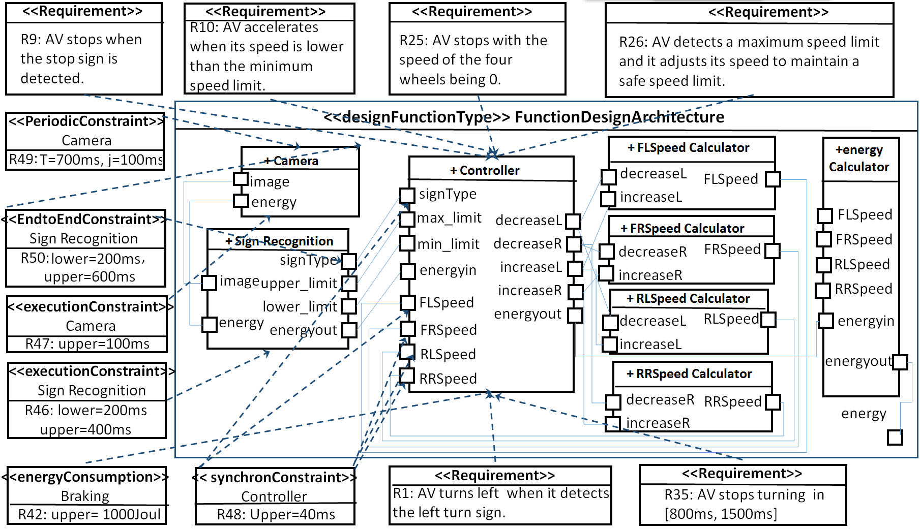
Figure 3.2: Design level East-adl model of AV

• R1. When the vehicle detects a left turn sign and it is going straight with a constant speed, it must turn towards left;

• R2. When the vehicle detects a left turn sign and it is accelerating, it must turn towards left;

• R3. When the vehicle recognizes a left turn sign and it is decelerating, it must turn towards left;

• R4. When the vehicle detects a right turn sign and it is going straight with a constant velocity, it must turn towards right;

• R5. When the vehicle recognizes a right turn sign and it is accelerating, it must turn towards right;

• R6. When the vehicle recognizes a right turn sign and it is decelerating, it must turn towards right;

• R7. When the vehicle detects a stop sign and it is going straight with a constant velocity, it must start to brake;

• R8. When the vehicle detects a stop sign and it is accelerating, it must start to brake;

• R9. When the vehicle detects a stop sign and it is decelerating, it must start to brake;

• R10. If the vehicle recognizes a minimum speed limit sign (70 or 80) when going straight with a constant speed, and the current velocity of the vehicle is smaller than the speed limit, the vehicle should accelerate;

• R11. If the vehicle recognizes a maximum speed limit sign (100 or 120) when going straight with a constant speed, and the current velocity of the vehicle is greater than the speed limit, the vehicle should decelerate;

• R12. If the vehicle recognizes a minimum speed limit sign (70 or 80) when it is decelerating, and the current speed of the vehicle is smaller than the speed limit, the vehicle should accelerate;

• R13. If the vehicle detects a minimum speed limit sign (70 or 80) when going straight with a constant speed and the current velocity of the vehicle is greater than the speed limit, it should maintain its speed;

• R14. If the vehicle detects a maximum speed limit sign (100 or 120) when accelerating, and the current velocity of the vehicle is greater than the limit, it must decelerate;

• R15. If the vehicle detects a maximum speed limit sign (100 or 120) when going straight with a constant velocity and its current velocity is smaller than the speed limit, the vehicle will maintain its speed;

• R16. When the vehicle detects a stop sign and it is turning left, it should decrease its speed and stop (the speeds of the four wheels should decelerate to 0);

• R17. When the vehicle detects a stop sign and it is turning right, it should decrease its speed and stop (the speeds of the four wheels should decelerate to 0);

• R18. When the vehicle recognizes a go straight sign and it is accelerating its speed, it should continue to accelerate.

• R19. When the vehicle recognizes a go straight sign and it is decelerating its speed, it should continue to decelerate;

• R20. When the vehicle is running at a high speed (i.e., the speed is greater than or equal to 70 m/s) and it detects a left turn sign, it should decelerate the speeds of the left wheels (in the front and rear) to turn towards left;

• R21. When the vehicle is running at a low speed (i.e., the speed of the vehicle is less than 70 m/s) and it detects a left turn sign, it will accelerate the speeds of the right wheels to turn towards left;

• R22. When the vehicle is running at a high speed and it detects a right turn sign, it should decelerates speeds of the right wheels to turn right;

• R23. When the vehicle is running at a low speed and it detects a right turn sign, it will accelerate the speeds of the left wheels to turn right;

• R24. When the vehicle is braking, it should finally stop with speeds of the four wheels 0;

• R25. When the vehicle decelerate to a full stop, the speeds of the four wheels should be 0;

• R26.When the vehicle detects a maximum speed limit sign with 100 as the limit, it automatically adjusts its speed to maintain a safe limit speed.

• R27.When the vehicle detects a maximum speed limit sign with 120 as the limit, it automatically adjusts its speed to maintain a safe limit speed.

• R28.When the vehicle detects a minimum speed limit sign with 70 as the limit, it automatically adjusts its speed to maintain a safe limit speed.

• R29.When the vehicle detects a maximum speed limit sign with 80 as the limit, it automatically adjusts its speed to maintain a safe limit speed.

• R30. When the vehicle is turning towards left, the speed of the wheels on the left side should be not greater than the speed of the wheels on the right side;

• R31. When the vehicle is turning towards right, the speed of the wheels on the right should be not greater than the speed of the wheels on the left side;

• R32. Once the vehicle starts to accelerate, it must complete its acceleration within certain time interval [0ms, 2400ms];

• R33. Once the vehicle starts to decelerate, it must complete its deceleration within certain time interval [0ms, 2400ms];

• R34. When the vehicle detects a stop sign, it must stop (the speeds of the four wheels become 0) within a certain time interval [0ms, 1200ms];

• R35. If the vehicle detects a left turn sign, it must turn left within a certain time interval [800ms, 1500ms];

• R36. If the vehicle detects a right turn sign, it must turn right within a certain time interval [800ms, 1500ms];

• R37. Energy constraint: The battery energy consumption for camera to captures an image should be within [1, 3] Joul;

• R38. Energy constraint: The battery energy consumption for computing the desired image (sign type) of an captured image in Sign Recognition should be within a certain interval [1, 5] Joul;

• R39. Energy constraint: The battery energy consumption for the vehicle to maintain a constant speed to go straight should be equal to the speed of the vehicle;

• R40. Energy constraint: The battery energy consumption for the vehicle to turn left should be within a certain interval [1, 270] Joul.

• R41. Energy constraint: The battery energy consumption for the vehicle to turn right should be within a certain interval [1, 270] Joul.

• R42. Energy constraint: The battery energy consumption for the vehicle to stop should be within a certain interval [1, 1000] Joul.

• R43. Energy constraint: The battery energy consumption for the vehicle to accelerate should be within a certain interval [0, 400] Joul.

• R44. Energy constraint: The battery consumption for the vehicle to decelerate should be within a certain interval [0, 400] Joul.

• R45. Energy constraint: When the velocity of vehicle is 0, the vehicle consumes no kinetics energy.

• R46. A Delay constraint applied on Sign Recognition $f_{p}$ is between 200 ms and 400 ms;

• R47. A Delay constraint applied on Camera is within 100 ms;

• R48. Synchronization constraint: The recognized sign types and the speeds of front/rear left/right wheels ( signType and F(R)L(R)Speed ports on Controller) must be detected by Controller within a given time window, i.e., the tolerated maximum constraint = 40 ms;

• R49. A Periodic acquisition of Camera must be vehicle should be carried out for every 700 ms with a jitter 100 ms.

• R50. A Delay is measured from Camera to Sign Type. The time interval is bounded with a minimum value of 200 ms and a maximum value of 600 ms;

• R51. The Delay from Camera to Sign Type should be less than or equal to the sum of the worst execution times of Camera and Sign Recognition.

According to the East-adl meta-model, the timing constraint describes a design constraint, but has the role of a property, requirement or validation result, based on its Context [5]. The Tadl2 meta-model is integrated with the East-adl meta-model and is supplemented with structural concepts from East-adl. The East-adl/Tadl2 constraints contain the identifiable state changes as Events. The causality related events are contained as a pair by EventChains. Based on Event and EventChains, data dependencies, control flows, and critical execution paths are represented as additional constraints for the East-adl functional architectural model, and apply timing constraints on these paths.

Delay constraint gives duration bounds (minimum and maximum) between two events source and target, i.e., period, end-to-end delays. This is specified using lower, upper values given as either Execution constraint (R46, R47) or End-to-End constraint (R50). Synchronization constraint describes how tightly the occurrences of a group of events follow each other. All events must occur within a sliding window, specified by the tolerance attribute, i.e., a maximum time interval allowed between events (R48). Repeat constraint states that the period of the successive occurrences of a single event must have a length of at least a lower and at most an upper time interval. The interval is given as Periodic constraint (R49). Those non-functional requirements (properties) are formally specified and verified in our approach using various analysis techniques that are described further in the following chapters.

Chapter 4 Modeling and Translation of East-adl Nonfunctional Properties in Simulink & Stateflow

4.1 Architectural Mapping to Simulink & Stateflow  using Metaedit+

Metaedit+  [18] tool provides .MDL export option to automatically generate MDL files from East-adl  model. The generated file of the East-adl model is an MDL file consisting of eight $<<$ Model Reference$>>$ blocks inside. The MDL file is mapped to the FunctionDesignArchitecture $F_{t}$ while each $<<$ Model Reference$>>$ blocks correspond to the $f_{p}$ with the identical name respectively.

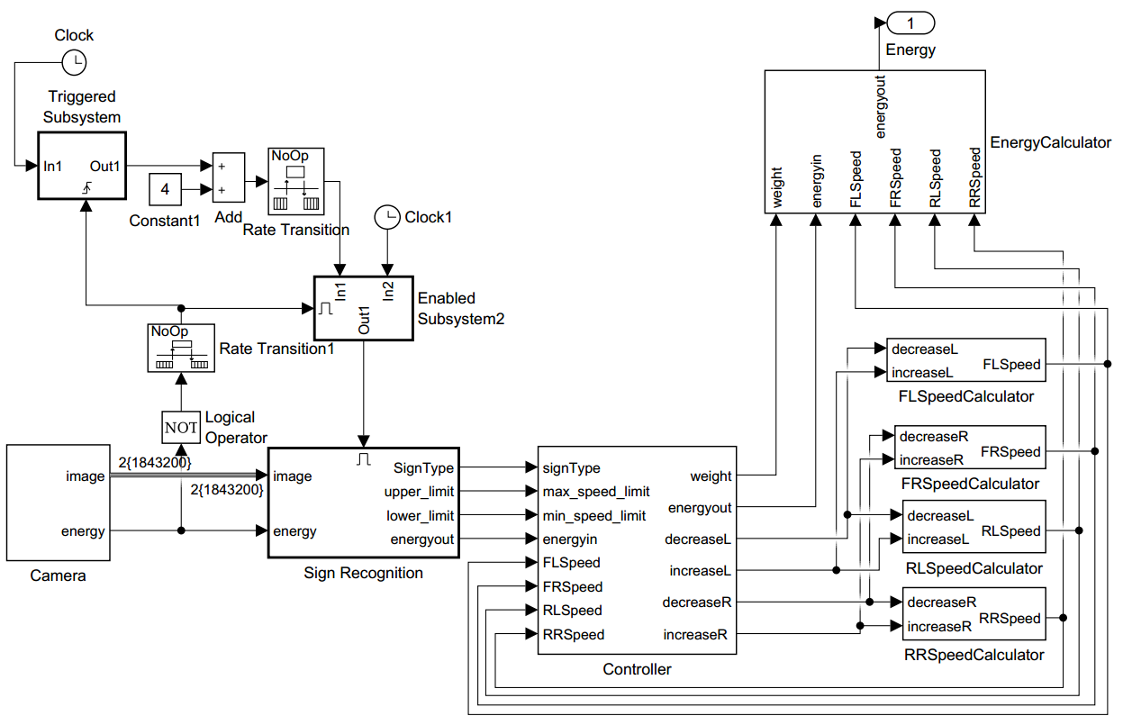
Figure 4.1: Simulink & Stateflow model of AV

The automatic model transformation is of great convenience for mapping architectural East-adl to Simulink/Stateflow model. However, if there are more than one connections from one output port in East-adl, after transformation, one of the connections may be lost in the exported model, which requests manual correction. As Fig.4.2 shows, the connection from upper_limit port to Controller is lost since there are two connections from the output port upper_limit.

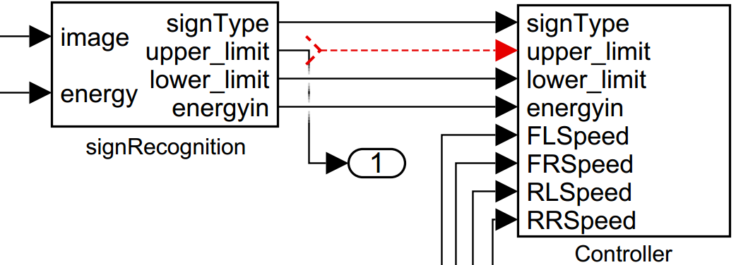
Figure 4.2: Error in generated model

4.2 Behavioral Modeling of $f_{p}$s in Simulink & Stateflow 

We refine the model and construct the behaviour of $f_{p}$s with Stateflow chart and Simulink blocks. Controller $f_{p}$ is modeled as a Stateflow chart while Camera, SignRecognition, Energy Calculator and (FL, FR, RL, RR) SpeedCalculator are modeled as subsystems with a number of descriptive blocks provided in Simulink block library. The architecture of Simulink/Stateflow model can be seen in Fig.4.1.

As shown in Fig.4.3, in Camera subsystem, a video is loaded from the workspace by using a $<<$ Multimedia File$>>$ block. Then Camera divides the source video into video frames (i.e. images) and output the frames to SignRecognition.

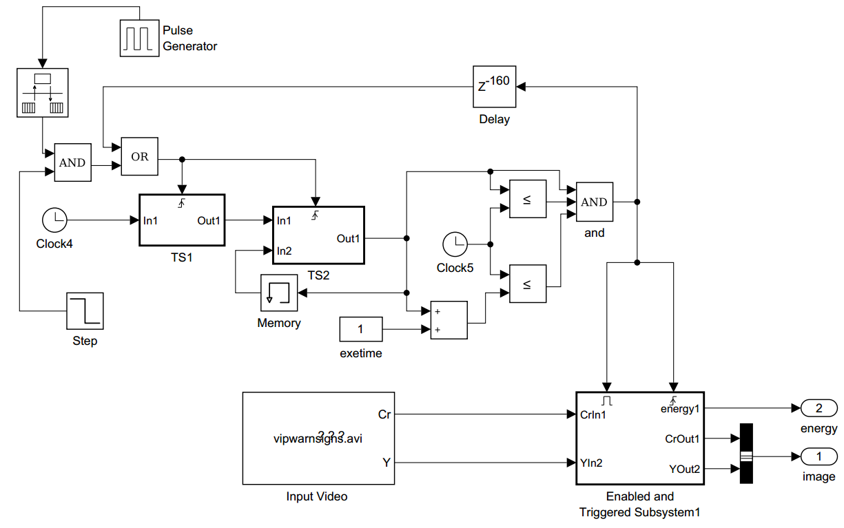
Figure 4.3: Simulink subsystem of Camera $f_{p}$

Fig. 4.4 illustrates the structure of SignRecognition subsystem, where the existed model for traffic warning sign recognition [19] provided by the Mathworks is applied and adapted. The model analyzes each input video frame in YCbCr color space. Y is the luma component and Cb and Cr are the blue-difference and red-difference saturability components. By thresholding and performing image processing on the Cr channel, the example extracts the outline of the key feature of the sign on the video frame. The model then compares the outline with each template signs stored in the Matlab workspace. If the outline is similar to any of the template signs, the model considers the most similar template to be the actual traffic sign.

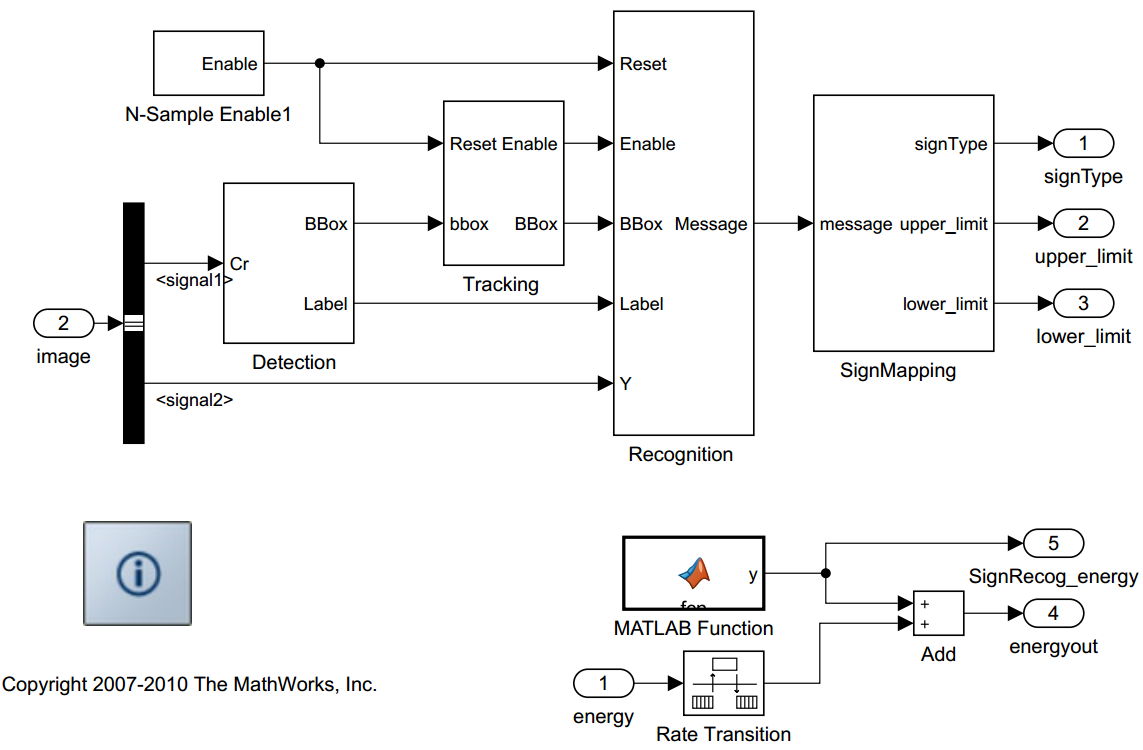
Figure 4.4: Simulink subsystem of SignRecognition $f_{p}$

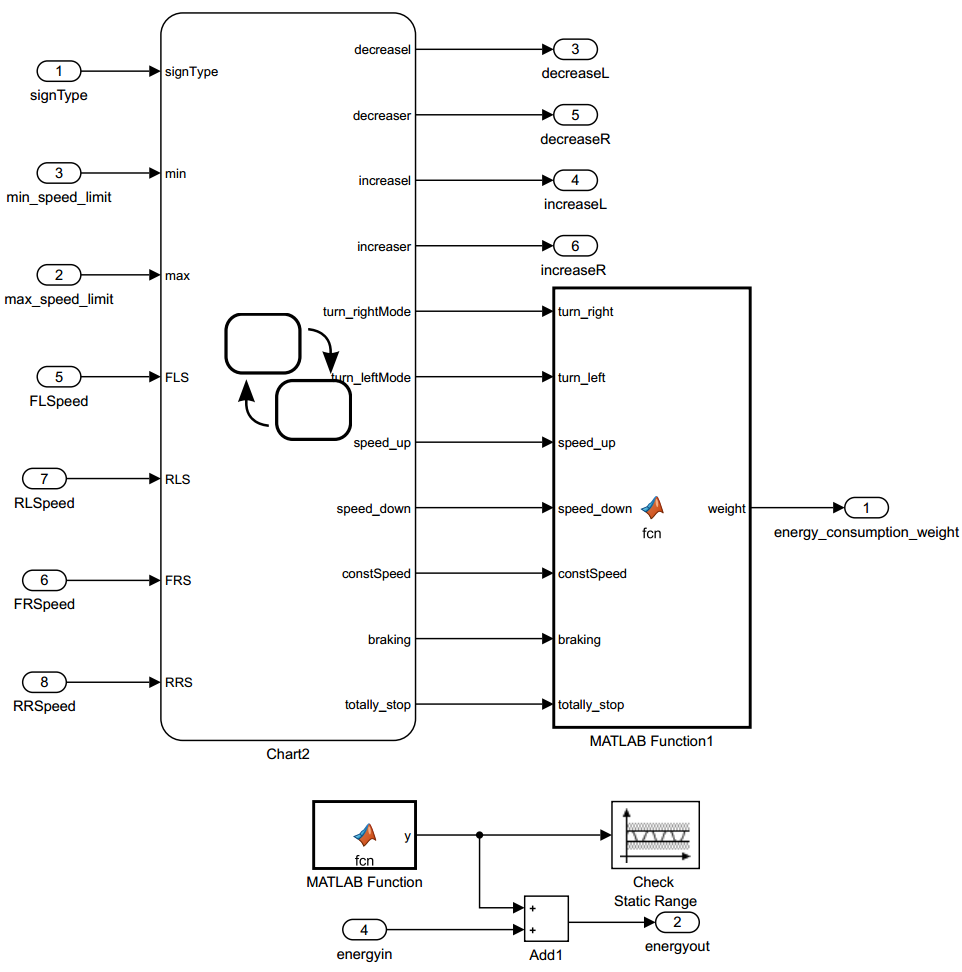
Figure 4.5: Simulink subsystem of Controller $f_{p}$

Controller subsystem is presented in Fig. 4.5 and the innner behaviour of Controller is illustrated in the Stateflow chart in Fig.4.7. The chart consists of four superstates turn_right, turn_left, straight, stop together with their child states. The edges represent transitions between the states with the conditions on the edges. The chart transits to either straight or stop based on the initial speeds of the wheels. The transitions will be taken according to the current speed of the wheels and the value of SignType. For example, when the vehicle is in speed_up state and the detected SignType is 5 (stop), braking and stop will be activated and decreaseL and decreaseR will become 1, indicating that the vehicle should decelerate the speeds of left wheels and right wheels. Whenever the vehicle detects a stop sign, the vehicle will start to brake. If the straight sign is detected, the vehicle will maintain the state/speed. If the vehicle recognizes a left turn sign, it can either decrease the speeds of the left wheels (in the front and rear) or increase the speed of right wheels to turn, which depends on whether the speed of the vehicle is greater than 70m/s. After turning left (right), the vehicle will finally go straight and maintain the speed. The embedded Matlab function checksign is applied to detect whether the stop sign is recognized when the vehicle is in the turning (left or right) mode.

SpeedCalculator subsystem calculates the speed of left (right) wheels. As shown in Fig. 4.6, in the FLSpeedCalculator subsystem, $<<$ Discrete-time Integrator$>>$ block and $<<$ Gain$>>$ operator are used to model the proportional relation between acceleration and speed. The value of the gain represents the acceleration of the movement (here is 8m/s²). The speed (of the front/rear left/right wheels ) is calculated based on the values of four boolean variables: increaseL, decreaseL, increaseR and decreaseR, whose value determine whether the acceleration is positive or negative. The same pattern can be applied for FRSpeedCalculator, RLSpeedCalculator and RRSpeedCalculator subsystems.

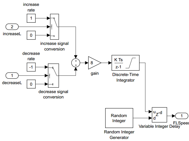
Figure 4.6: Simulink subsystem of FLSpeedCalculator $f_{p}$

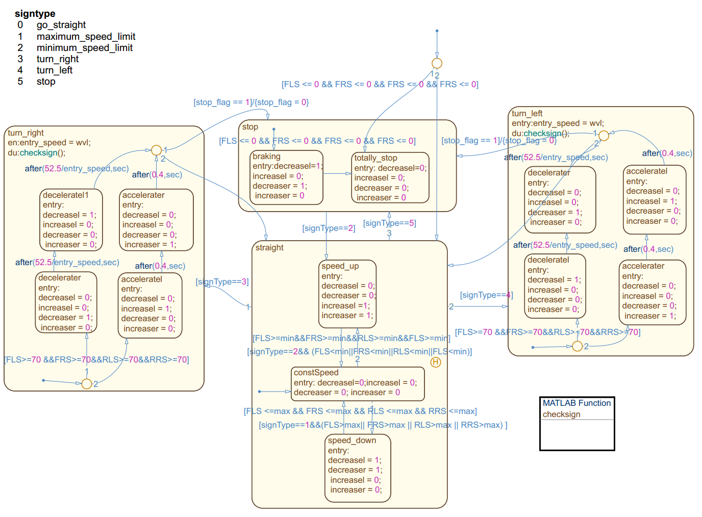
Figure 4.7: The Stateflow of Controller $f_{p}$

4.3 Timing and Energy Constraints Translation

Timing and energy constraints in East-adl are modeled by means of constraints specified on events and event chains. We show how the East-adl constraints can be interpreted in Simulink/Stateflow (S/S) and provide corresponding modeling extensions in S/S. We focus on Synchronization, Execution, End-to-End, Periodic constraints (R46 to 51) and energy consumption constraints (R42) that are associated to $f_{p}$s in East-adl. Additionally, we provide sufficient means to specify trigger conditions for:

1. Time-triggered $f_{p}$ is triggered every period T. We use sample time and set sample time = T for the block which corresponds to the $f_{p}$ in S/S. For example, Camera $f_{p}$ takes a picture every 20ms, the sample time of Camera block is set to 20ms, i.e., the block is executed every 20ms.

2. Event-triggered $f_{p}$. The condition is expressed by a set of ports, i.e., at least one data/event must be received/occured on each port after the last $f_{p}$ execution in order to trigger the $f_{p}$ again. It can be modeled as Trig_sub in S/S  (Fig.4.8). A trigger event is on an event_trig_in port, i.e., whenever an event occurs, the input signal of event_trig_in becomes true and Trig_sub is activated.

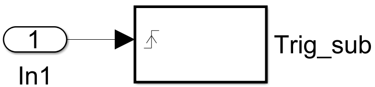
Figure 4.8: Event triggered timing constraint translation pattern

Execution constraints: In terms of Time- or Event-triggered $f_{p}$, two types of execution timing constraint translation patterns are provided: (1) Time-triggered $f_{p}$ translation pattern is shown in Fig.(a). Pulse Generator generates signals (square waves) based on Amplitude, Period, Pulse width parameters (Fig.4.9.(b)). Pulse width is a duty cycle specified as a percentage of Period. Enabled Subsystem (representative of $f_{p}$) is executed when the triggering signal is greater than zero. Hence, the execution time of Enabled Subsystem is $Pulsewidth*Period$ in this pattern; (2) Event triggered $f_{p}$ translation pattern is shown in Fig.4.9.(c). Trigg- ered Subsystem is triggered by the rising edge of the square wave (changing curve from 0 to 1), where the rising edge indicates an event occurrence from input port 1, Clock outputs the current time instance, and $exetime$ is Execution time constraint. For example, an event occurs and Triggered Subsystem is triggered at the t time point. In the meantime, the value of In1 of Compare becomes t+exetime. If the current time instance is in [t, t+exetime] (i.e., the current time is within the range of execution timing constraint), Out1 becomes true and Enabled Subsystem is executed.

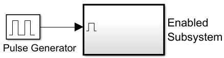
(a) Time-triggered $f_{p}$ Translation

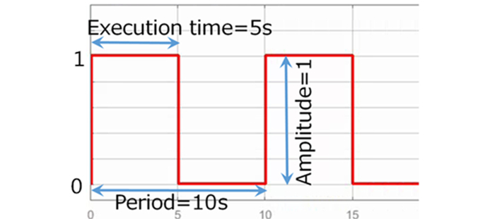
(b) Signal from Pulse Generator

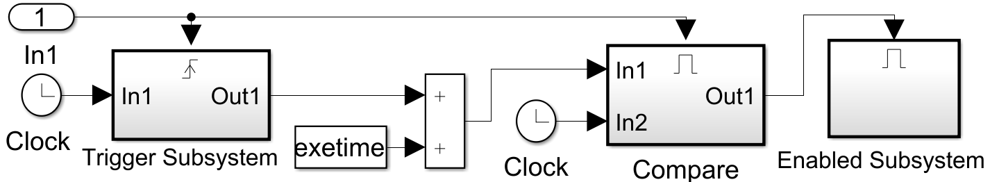
(c) Event-triggered $f_{p}$ Translation

Figure 4.9: Execution timing constraint translation patterns

Synchronization constraint is a constraint on a set of events, which restricts the time duration among the $n^{th}$ occurrence of all the events in the set (i.e., maximum allowed time between the arrival of the event occurrences). The translation pattern for Synchronization constraint is illustrated in Fig.4.10. An observer Stateflow is used to record the exact arrival time of each event occurrence. A Synchronization constraint (attached to the Controller $f_{p}$ in Fig.3.2) is the maximum tolerated time difference among the arrivals of recognized sign types and the speeds of left/right wheels (R48). To calculate the time interval between the earliest and latest arrivals, the observer Stateflow (Chart) is connected to Controller in Fig.4.10. The five inputs of Chart, $s_{1}$ represents a parameter (signal) of a sign type, and $s_{2},s_{3},s_{4},s_{5}$ denote the speed of the four wheels respectively. $o_{i}$ records the history value of each $s_{i}$, where $i=1,2,3,4,5$. $u_{i}$ indicates if the signal has updated (changed). A boolean y indicates if the calculated time interval meets the synchronization constraint. The arrival of each $s_{i}$ is monitored by comparing the current and previous values of the $s_{i}$ in judge function. If any $s_{i}$ is updated, the initial state is changed to start. If the other remained signals are subsequently updated within the synchronization constraint, y is set to 1. A graphical illustration of $s_{i}$ is given in Fig.4.10.(b), where, $t(s_{i})$ is a time point of the $i^{th}$ occurrence of $s$. Similarly, a consecutive event of $s_{i}$ and its time point can be shown as $s^{\prime}_{i}$ and $t^{\prime}(s_{i})$. Recall R48, the difference among $t(s_{i})$ and their consecutive events must be within the maximum tolerance (40ms).

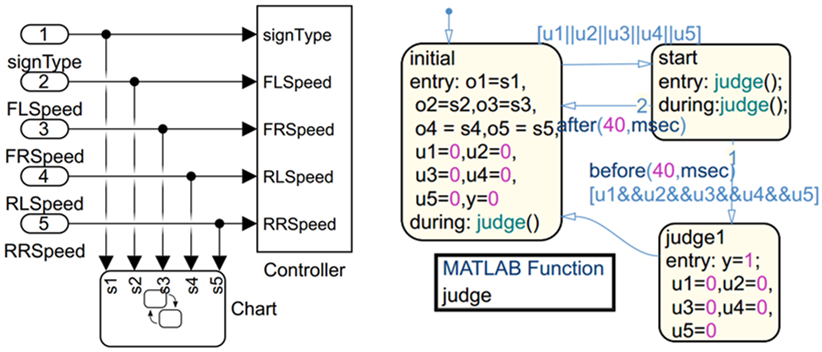
(a) Synchronization timing constraint translation pattern

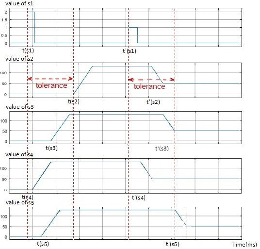
(b) Signal examples

Figure 4.10: Synchronization timing constraint translation pattern and signal examples

Periodic constraint restricts the period of successive occurrences of $f_{p}$ within a time interval [$T-j$, $T+j$], where $T$ and $j$ are a period and a jitter. The translation pattern is shown in Fig.4.11: An enabled subsystem, ES, which corresponds to $f_{p}$, is triggered by signals from two subsystems, TS1 and TS2. $t_{i}$ denotes a time point of the $i^{th}$ triggered ES (i.e., $i^{th}$ occurrence of $f_{p}$). To calculate $t_{1}$, Pulse Generator and Step blocks trigger TS1 and TS2 at time T-j. TS1 sends the current time T-j to TS2. Since $f_{p}$ can be triggered at any time point in [-j, j], TS2 generates a value $r_{i}$ $\in$ [0, 2j]. According to the pattern, the $1^{st}$ occurrence of $f_{p}$ happens at $t_{1}$ $=$ $T-j+r_{1}$, where $t_{1}$ $\in$ $[T-j,T+j]$. Similarly, the time point of each consecutive $f_{p}$ occurrence ($t_{2}=t_{1}+T-j+r_{2}$, $t_{3}=t_{2}+T+j+r_{3}$, etc.) can be calculated. The Delay block ensures that $t_{i}$ must be calculated prior to its lower bound ($t_{i-1}+T-j$). In order to guarantee $f_{p}$ is executed periodically, the execution timing constraint translation pattern is applied (exetime). Using this pattern, R49 is validated in section 6.

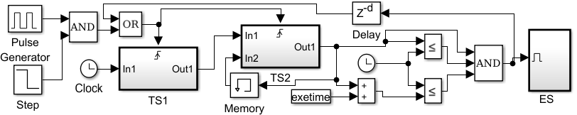
Figure 4.11: Periodic timing constraint translation pattern

End-to-End constraint specifies how long after the occurrence of a stimulus, a corresponding response must occur. The input and output of a block ($B$) in S/S are triggered by sample time ($st$). Assume that $B_{1}$/$B_{n}$ is the first (stimulus)/last (response) block of a series of connected blocks. $B_{i}$ is the $i^{th}$ block and its sample time is ${st}_{i}$. In Simulink, a time interval between $B_{1}$ (where the inputs arrive) and $B_{n}$ (from where the outputs leave) is $s_{sum}$ $=$ $\sum_{i=1}^{n}s_{i}$. In the case that $B_{i}$ finishes its execution before $B_{i}$ is triggered again (i.e., the execution time of $B_{i}$ is shorter than its triggered time interval), End-to-End constraint (the sum of all execution times of each $B_{i}$) can be less than or equal to $s_{sum}$. Therefore, End-to-End constraint cannot be expressed in S/S using sample times. The following sections elucidate how this constraint can be modeled alternatively and analyzed.

Energy constraint is associated to each $f_{p}$ to restrict minimum/maximum resource allocation on the execution platform. The energy consumption of either the $f_{p}$ or the whole systems consisting of $f_{p}$s is modeled using differential equation blocks in Simulink. According to the various modes of AV, the amount of battery power expended for the mechanical motion of the wheels is calculated:

$$energy=\int_{0}^{t}a*vdx$$

where, $t$, $a$, and $v$ denote running time, coefficient reflects an energy rate associated to the current mode of AV, and wheel speed respectively. Details of energy-aware analysis is presented in chapter 6.

Chapter 5 Modeling and Translation of East-adl  Nonfunctional Properties in Uppaal-smc

5.1 Architectural and Behavioral of East-adl  and Simulink & Stateflow  to Uppaal STA

To translate the dynamic and continuous behaviours of Camera and SignRcognition subsystems to Uppaal-smc, we use and modify the interface automaton (Fig. 5.1(a)) proposed in our previous work [20]. Read and Write locations are committed to guarantee that there is no delay or interruption. Then, we capitalizes on the automatic code generation function in Matlab and generate c code using Simulink Coder. The code is modified and embedded in SignRec function in the automaton. The automaton reads images data via PortIn? channel. After getting inputs, the automaton will execute and update the values of signType, lower_limit and upper_limit. These parameters and signals are then written to output port, and the automaton will return to Idle and wait for another trigger from the previous blocks. The STA shown in Fig.5.2(a) preserve the behaviour of Camera $f_{p}$. Fig.5.2(b) illustrates the STA that used for modeling the contimuous behaviour of four SpeedCalculator $f_{p}$s.

To model the stochastic behaviours of SignRecognition $f_{p}$ that the traffic sign occurs randomly, a STA with eight non-deterministic edges is used (Fig.5.1(b)). The eight edges corresponding to eight signs are associated with probability weight (here 0.3 for straight sign and 0.1 for the each of the other seven signs), which means that a discrete probabilistic choice ($\frac{30}{100}$ for straight sign versus $\frac{10}{100}$ for the other seven signs) is made.

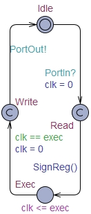
(a) TA

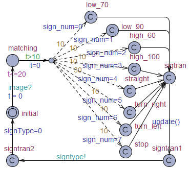
(b) Random generation of signType with probabilistic distribution

Figure 5.1: Translate Simulink/Stateflow model to Uppaal STA

We translate the Stateflow chart into Uppaal-smc STA by applying the methodology in [20]. The Stateflow chart is translated into 5 STAs: Controller, Stop, Straight, Turn_left and Turn_right respectively. Controller STA corresponds to the topmost superstate of the Stateflow and it contains 4 locations: turn_left/right, stop, straight. Each location is mapped to the the STA with the identical name. As shown in Fig.5.3 to Fig.5.6, each STA has an initial location. Controller interacts with other STA (representatives of child states in Stateflow chart) via synchronization channels. For example, if Controller stays in turn_left location, the initial location of Turn_left STA will be inactive. At the same time, the other three STAs, i.e. Turn_right, Straight and Stop STA should stay in their initial state respectively.

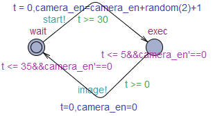
(a) STA of Camera $f_{p}$

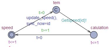
(b) STA of SpeedCalculator $f_{p}$

Figure 5.2: Model the continuous behaviour of Simulink/Stateflow in Uppaal

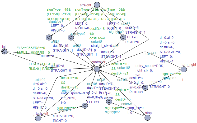
Figure 5.3: STA of Controller

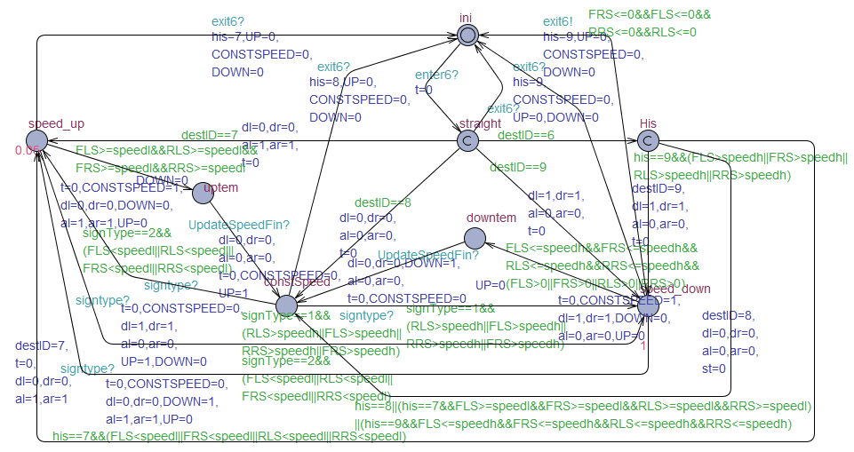
Figure 5.4: STA of straight state in Controller

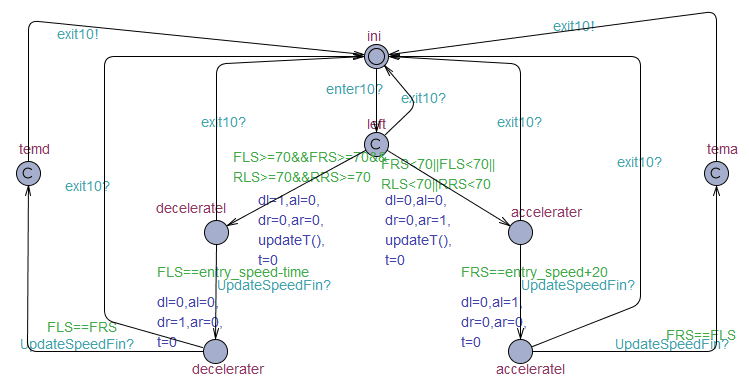
(a) STA of turn_left state

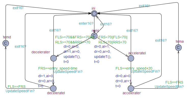
(b) STA of turn_right state

Figure 5.5: STA of turn_left and turn_right state in Controller

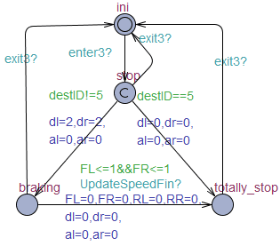
Figure 5.6: STA of stop state in Controller

5.2 Probabilistic Timing Constraints Translation

We discuss semantics of the extended Execution, Synchronization, Periodic, and End-To-End timing constraints (Xtc) with probabilistic parameter according to Tadl2 [7]. Afterwards, we provide Xtc translation in STA and discuss it with the view point of analysis engine Uppaal-smc. Xtc and its translation follow the weakly-hard (WH) approach [7], which describes a bounded number of all event occurrences are allowed to violate the constraints within a time window. The semantics of the WH(c,m,K) is that a system behavior must satisfy a given timing constraint c at least m times out of k consecutive occurrences of events. We use object-oriented notation to define the attributes of occurrences of an event. These attributes are time points showing when instances of the event happens, e.g., $f_{p}$.response refers to the time at which the response event of $f_{p}$ is specified.

WH(Execution,m,k) limits the time between the starting and stopping of an executable $f_{p}$ following run-to-complete semantics, i.e., not counting the intervals when the executable $f_{p}$ has been interrupted. At least m times out of k consecutive occurrences of the event, $f_{p}$.start, satisfy: lower $\leq$ $\mid$ $f_{p}$.stop $\setminus$ ( $f_{p}$.preempt, $f_{p}$.resume)$\mid$ $\leq$ upper, where lower (upper) denotes the time point showing when the $f_{p}$ starts (stops). The STA modeling of $f_{p}$’s execution constraint is shown in Fig.5.7.(a). The STA is executed via input[id]? and its completion is updated via output[id]?. The execution time of $f_{p}$ (execclk) is calculated in the exec location. When $f_{p}$ is started, a local clock execclk is reset. If $f_{p}$ is preempted (input[e]?), execclk holds (rate = 0) until the $f_{p}$ is resumed. When $f_{p}$ is completed, STA moves to finish location and it determines if execclk is within the given Execution constraint. In case of satisfying the constraint, it moves to success location, otherwise stays in fail location. The interpretation of WH(Execution,m,k) is given as a Hypothesis Testing query in Uppaal-smc and it is as follows, $P$: $Pr[bound]$ ($[\ ]\neg$$STA_{Execution}.fail$) $\geq$ $P$, where bound and $P$ indicate the time bound on the simulation and $\frac{m}{k}$ respectively.

WH(Synchronization,m,k): A set of input events of an $f_{p}$ constrains the maximum allowed time delay attribute, tolerance, among the arrival of the event occurrences. For any event e in the set s.t. the fastest arrival event (e(i).fastest) and the slowest arrival event (e(j).slowest), where i $\neq$ j, at least m times out of k consecutive occurrences of the set satisfy $\mid$ e(j).slowest-e(i).fastest$\mid$ $\leq$ tolerance. The corresponding STA in Fig. 5.7.(b) specifies the time width within which a set of ”input” event should occur. For simplicity, we assume three input events occur (denoted source[e]?). The parameter syn_upper (represented as tolerance) determines the maximum timed allowed among the three inputs. WH(Synchro- nization,m,K) is specified as $P$: $Pr[bound]$ ($[\ ]$ $\neg$ $STA_{Synchronization}.fail$) $\geq$ $P$. Output synchronization constraint translation is similar to the input synchronization except that instead of ”input”, ”output” are constrained to occurred in a specified time width.

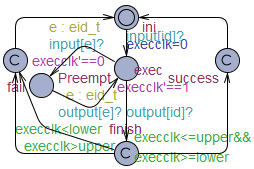
(a) Execution

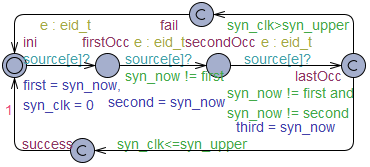
(b) Synchronization

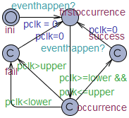
(c) Periodic

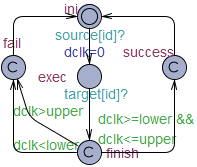
(d) End-to-End

Figure 5.7: STA of East-adl/Tadl2 Probabilistic Extension of Timing Constraints

WH(Periodic,m,k) limits the period of the successive occurrences of a single event $f_{p}$ including jitter. For any s(i) $\in$ $f_{p}$.start s.t. its successive occurrence s’(i) starting at s(i), out of k consecutive occurrences s(i), i.e., s(i) to s(i+k), at least m sequences satisfy (T-jitter $\leq$ $\mid$s’(i)-s(i)$\mid$ $\leq$ T+jitter) $\land$ ( lower $\leq$ T $\leq$ upper), where T denotes a bounded length of at least a lower and at most an upper time interval, given as the period without jitter. The STA in Fig. 5.7.(c) enforces the event eventhappen to arise within the bounded time interval between every two consecutive occurrences of it. When the $1^{st}$ occurrence happens, STA resets its local clock ($pclk$) and starts counting until the $2^{nd}$ occurrence happens. Afterwards, it judges if $pclk$ is within the periodic constraints and changes its current state to either (success or fail) based on the judgement. Finally, STA returns to firstocccurrence and repeats the calculation on the next two consecutive occurrences of the event. WH(End-to-End,m,k) is specified as $P$: $Pr[bound]$ ($[\ ]$ $\neg$$STA_{Periodic}.fail$) $\geq$ $P$.

WH(End-to-End,m,k) limits tolerance between the occurrences of two events ($f_{p}$s) source, target. Only one-to-one occurrence patterns are allowed. For any s $\in$ $f_{p}$.source s.t. s=source(i) for some i $\leq$ $\mid$source$\mid$, out of k consecutive occurrences s of $f_{p}$.source, i.e., source(i) to source(i+k), at least m satisfy lower $\leq$ $f_{p}$.target(i)-s $\leq$ upper, where $f_{p}$.target(i)-s denotes the corresponding delay of $f_{p}$.source(i). The STA in Fig. 5.7.(d) specifies tolerance between $f_{p}$.source and $f_{p}$.target. dclk counts the delay ( tolerance) based on inputs via source[id]? and target[id]?. After allowing one-to-one source and target occurrence patterns, STA changes its state to finish and decides its successor location either success or fail based on checking if dclk is within the End-to-End constraint. The interpretation of WH(End-to-End,m,k) is given as a query, $P$: $Pr[bound]$ ($[\ ]$ $\neg$$STA_{End-to-End}.fail$) $\geq$ $P$.

5.3 Energy-aware Modeling and Estimation

In order to estimate the energy consumption of hybrid AV based on Xtc and energy constraints, the Controller $f_{p}$ (which consumes batteries differently on variant modes) is selected and its ERT behaviors are formally specified in STA. The STA of Controller (Fig.5.8) presents stochastic hybrid behaviors with extended arithmetic on clocks and their rates: Con_en (defined as an ODE and assigned at each location). Different locations in the STA correspond to (one or two) states of Controller (visualized in Stateflow in Fig.4.7). A pair of modes having the same energy consumption rate can be combined into one and depicted as a location, i.e., since the energy consumption rates of turn_left/right modes are the same, they are expressed as a turnLeftorRight location in STA. Because the energy consumption rate varies in different running mode, e.g., the energy is consumed fast when the vehicle is in braking mode and slowly in constSpeed mode. We define Con_en’ (the rate of Con_en ) with ordinary differential equation (ODE) and assign different values to Con_en’ for different locations. UpDownRate, BrakingRate, ConstSpeedRate and TurningRate are user-supplied coefficients in ODE that represent battery consumption and its various rates on different modes respectively and BrakingRate $>$ UpDownRate $>$ TurningRate $>$ ConstSpeedRate. The value of the coefficients indicate the rapidity of the energy consumption. The estimation of energy consumption requirement of Controller will be evaluated in chapter 6.

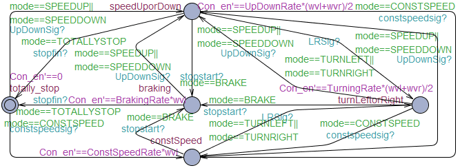
Figure 5.8: STA of the energy consumption of Controller

Chapter 6 Experiments: Verification & Validation

We employ Uppaal-smc and SDV for the verification and Matlab/Simulink for the simulation of functional (R1–R36) and timing- and energy constraints properties (R37–R51).

6.1 SDV verification

Fig. 6.1(b) illustrates an example model of non-temporal functional requirement in SDV. The value of SignType signal ranges from 0 to 5, which represents straight sign, maximum/minimum speed limit sign, turn right/left sign and stop sign respectively. In Fig.6.1(a), lower_limit, upper_limit and SignType are constrained in $<<$ Proof Assumption$>>$ block such that the signal must match one of the listed values at every time step, i.e., sample interval. The states in Stateflow chart are output as boolean signals for monitoring, e.g., the value of straight is 1 when state straight is active and 0 otherwise. A $<<$ Detector$>>$ block is applied to add a unit time delay for condition, suggesting that the condition should be true at previous time step.

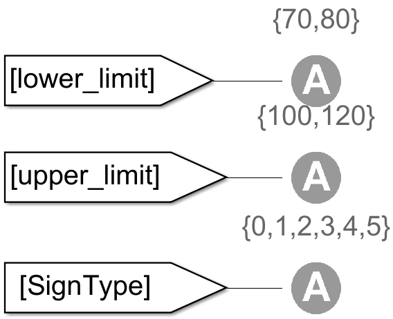
(a) Input constraint

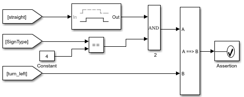
(b) Model of requirement

Figure 6.1: Example model of non-temporal functional property: If straight state is active and SignType is 4, turn_left state should be active next time step.

The temporal functional requirement can be model as Fig. 6.2. As shown in Fig.6.2(b), once the chart exits turn_left, temporalCount(msec) (which is an expression in absolute time temporal logic) returns the integer number of milliseconds that have elapsed since activation of the turn_left state (i.e, the time duration of turning left). Then the action assigns to T_left, which is an output variable to Simulink indicating the time duration of turning left.

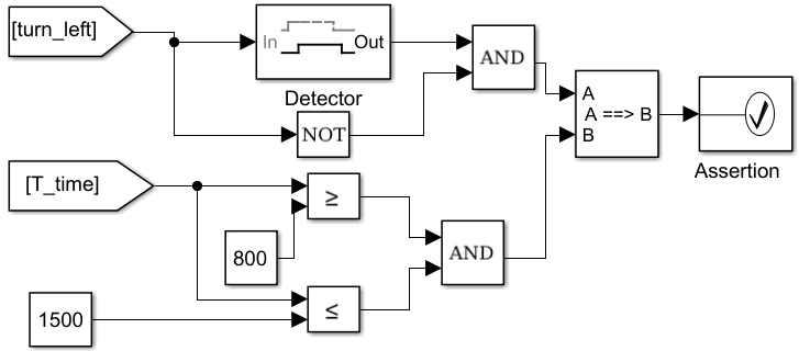
(a) Model of requirement

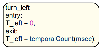
(b) temporalCount

Figure 6.2: Example model of temporal functional property: If turn_left state is active at previous time step and inactive at current time step, T_left should be between 800 and 1500 (The time duration for turning left should be between 800 and 1500 ms).

The proof objective model of the requirement R7 is presented below.

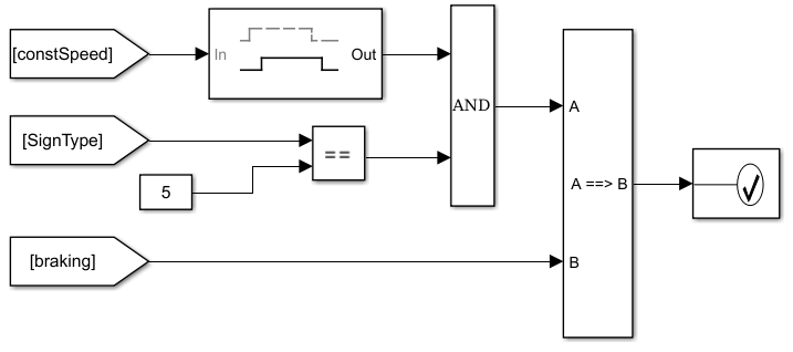
Figure 6.3: Model of requirement R7: If constSpeed is active and the detected SignType is 5, then the system will enter the braking state in the next time step.

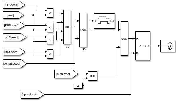
Figure 6.4: Model of requirement R10: If the vehicle detects minimum speed limits sign when constSpeed state is active, and its speed is less than the speed limit (SignType equals 2), speed_up state will be activated in the next time step.

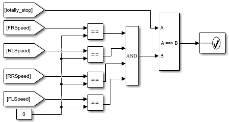
Figure 6.5: Model of requirement R25: When totally_stop state is active, the speed of the four wheels of the vehicle should be zero.

The non-functional properties includes energy properties and temporal properties. SDV is not applicable for verifying the timing constraints and energy properties because it lacks descriptive blocks for constructing the requirements. For constructing the timing constraints, to detect the time instant of the input arrival or the output departure, the trigger-based blocks should be applied. However, SDV does not support the trigger-based blocks. Moreover, when modeling the behaviour of energy consumption, we add the stochastic elements (blocks/algorithms), which is not supported in SDV, either.

Table LABEL:table_verification_result (where the variables with prime represent variables in the previous time step) shows the verification result of the requirements. For the functional properties that are not related to time (R1 to R25, R30 and R31), the verification results are all valid in SDV. SDV cannot provide the verification results (valid or not) of R32 to R36 because the verification time exceeds the user-defined maximum analysis time (here it is set as 50 minutes).

6.2 UppaalVerification and Simulation

A validation of the translation patterns becomes a reachability analysis in the following forms: 1. $A[\ ]$$\neg$$deadlock$verifies that a system is free of any inconsistencies iff there is no deadlock and all the constraints modeled in STA through the mapping strategy are satisfied; 2. $A[\ ]$$\neg$$(STA.fail)$, where $fail$ is a location containing constraints that are not satisfied. It verifies that a given constraint modeled with an STA never reaches the $fail$ location.

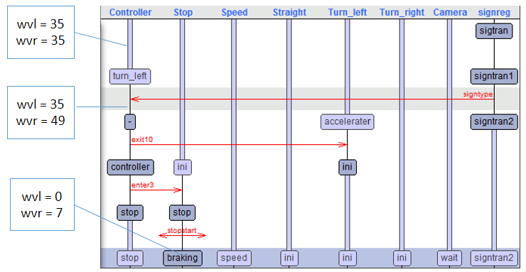
Figure 6.6: CE in Uppaal-smc: Initially, Controller transits to turn_left. When Turn_left stays in accelerater location, the wvr is increased while wvl is constant. When the vehicle detects a stop sign and brakes to stop, finally wvl is 0 but wvr is larger than 0 hence violates R16.

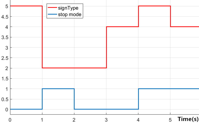
(a) signType and stop mode

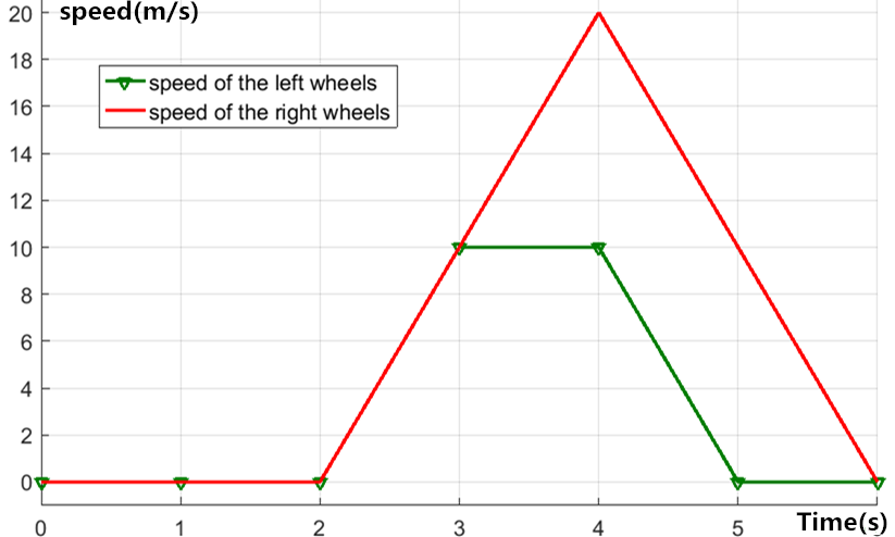
(b) speeds of the left/right wheels

Figure 6.7: CE in SDV: signType is turn left (4) at 3s and becomes stop (5) at 4s. Then the vehicle enters stop mode and decreases speeds of the left and right wheels. However, at 5s, the speed of the left wheels is 0 while the speed of the right wheels is greater than 0, which disproves R16.

When verifying R16, it is proved that R16 is invalid in both SDV and Uppaal-smc. By tracing the counter-example illustrated in Fig.6.6 and Fig.6.7, we can find the reason of the invalidity: If the vehicle detects a stop sign when turning left/right, it will enter stop state with the speeds of the left/right wheels unequal. Since the acceleration of the wheels are identical, the speed will not be decreased to zero simultaneously. We refine the requirement of R16 as: when the vehicle detects a stop sign when turning left/right, it should first finish the turning and then stop. The requirement becomes valid after modifying the model.

Table 6.1: Logic expression and verification results

Req	Type	Expression	Result	Time (min)	Memory (Mb)	CPU (%))
R1	SDV	${\mathop{constspeed^{\prime}}==true\wedge signType==4\implies turn\_left==true}\$	valid	6	1834	40.17
	Uppaal-smc	${Pr[\leqslant 3000]([\ ](CONSTSPEED==1\wedge signType==4}{\wedge\neg Ctrl.ctrl}$ $\wedge Ctrl.t==0){\implies}{Ctrl.turn\_left)\geqslant 0.95}$	valid	0.002	30.91	1.2
R2	SDV	${\mathop{speed\_up^{\prime}}==true\wedge signType==4\implies turn\_left==true}$	valid	6.25	1855	39.61
	Uppaal-smc	${Pr[\leqslant 3000]([\ ](SPEEDUP==1\wedge signType==4}\wedge\neg Ctrl.ctrl$ $\wedge Ctrl.t==0)\implies{Ctrl.turn\_left)\geqslant 0.95}$	valid	0.002	30.91	1.2
R3	SDV	${\mathop{speed\_down^{\prime}}==true\wedge signType==4\implies turn\_left==true}$	valid	6.25	1849	39.30
	Uppaal-smc	${Pr[\leqslant 3000]([\ ](SPEEDDOWN==1\wedge signType==4\wedge}\neg Ctrl.ctrl$ $\wedge Ctrl.t==0){\implies}{Ctrl.turn\_left)\geqslant 0.95}$	valid	0.002	30.91	1.2
R4	SDV	${\mathop{constspeed^{\prime}}==true\wedge signType==3\implies turn\_right==true}$	valid	6.30	1872	39.42
	Uppaal-smc	${Pr[\leqslant 3000]([\ ](CONSTSPEED==1\wedge signType==3}{\wedge\neg Ctrl.ctrl}$ $\wedge Ctrl.t==0)\implies{Ctrl.turn\_right)\geqslant 0.95}$	valid	0.003	31.02	1.3
R5	SDV	${\mathop{speed\_up^{\prime}}==true\wedge signType==3\implies turn\_right==true}$	valid	6.46	1872	40.14
	Uppaal-smc	${Pr[\leqslant 3000]([\ ](SPEEDUP==1\wedge signType==3}{\wedge\neg Ctrl.ctrl}$ $\wedge Ctrl.t==0)\implies{Ctrl.turn\_right)\geqslant 0.95}$	valid	0.003	31.02	1.3
R6	SDV	${\mathop{speed\_down^{\prime}}==true\wedge signType==3\implies turn\_right==true}$	valid	7.04	1895	40.16
	Uppaal-smc	${Pr[\leqslant 3000]([\ ](SPEEDDOWN==1\wedge signType==3\wedge}\neg Ctrl.ctrl$ $\wedge Ctrl.t==0)\implies{Ctrl.turn\_right)\geqslant 0.95}$	valid	0.003	31.02	1.3
R7	SDV	${\mathop{constspeed^{\prime}}==true\wedge signType==5\implies braking==true}$	valid	8.47	1953	39.61
	Uppaal-smc	${Pr[\leqslant 3000]([\ ](signType==5\wedge CONSTSPEED==1\wedge}\neg Ctrl.ctrl$ $\wedge{Ctrl.t==0)\implies Ctrl.stop)\geqslant 0.95}$	valid	0.003	30.91	1.3
R8	SDV	${\mathop{speed\_up^{\prime}}==true\wedge signType==5\implies braking==true}$	valid	8.47	1953	39.61
	Uppaal-smc	${Pr[\leqslant 3000]([\ ](signType==5\wedge SPEEDUP==1\wedge}\neg Ctrl.ctrl$ $\wedge{Ctrl.t==0)\implies Ctrl.stop)\geqslant 0.95}$	valid	0.003	30.91	1.3
R9	SDV	${\mathop{speed\_down^{\prime}}==true\wedge signType==5\implies braking==true}$	valid	6.36	1905	39.39
	Uppaal-smc	$Pr[\leqslant 3000]([\ ](signType==5\wedge SPEEDDOWN==1\wedge\neg Ctrl.ctrl$ $\wedge{Ctrl.t==0)\implies Ctrl.stop)\geqslant 0.95}$	valid	0.003	30.91	1.3

Req	Type	Expression	Result	Time (min)	Memory (Mb)	CPU (%))
R10	SDV	$constspeed^{\prime}==true\wedge signType==2{\wedge(FLS<min\vee FRS<min}\vee RLS<min\vee RRS<min)\implies{speed\_up==true}$	valid	7.18	1894	39.28
	Uppaal-smc	${Pr[\leqslant 3000]([\ ](Straight.CONSTSPEED==1\wedge sign==2}\wedge(FLS<speedl\vee FRS<speedl\vee RLS<speedl\vee RRS<speedl)\wedge Straight.t==0)\implies Straight.speed\_up)\geqslant 0.95$	valid	0.003	30.92	1.4
R11	SDV	${constspeed^{\prime}}==true\wedge signType==1\wedge(FLS>max\vee FRS>max\vee RLS>max\vee RRS>max)\implies speed\_down==true$	valid	6.40	1931	39.43
	Uppaal-smc	$Pr[\leqslant 3000]([\ ](Straight.CONSTSPEED==1\wedge sign==1\wedge(FLS>speedh\vee FRS>speedh\vee RLS>speedh$ $\vee RRS>speedh)\wedge Straight.t==0)\implies Straight.speed\_down)\geqslant 0.95$	valid	0.002	30.92	1.2
R12	SDV	$\mathop{speed\_up^{\prime}}==true\wedge signType==1\wedge(FLS>max\vee FRS>max\vee RLS>max\vee RRS>max)\implies speed\_down$	valid	11.58	1977	37.41
	Uppaal-smc	$Pr[\leqslant 3000]([\ ](Straight.UP==1\wedge sign==1\wedge(FLS>speedh\vee FRS>speedh\vee RLS>speedh\vee RRS>speedh)\wedge Straight.t==0)\implies Straight.speed\_down)$	valid	0.002	30.95	22.24
R13	SDV	$constspeed^{\prime}==true\wedge signType==2\wedge FLS\geqslant min\geqslant FRS\geqslant min\wedge RLS\geqslant min\wedge RRS\geqslant min\implies constspeed$	valid	5.37	2085	39.05
R14	SDV	$speed\_down^{\prime}==true\wedge signType==2\wedge(FLS<min\vee FRS<min\vee RLS<min\vee RRS<min)\implies speed\_up$	valid	10.21	1947	38.93
	Uppaal-smc	$Pr[\leqslant 3000]([\ ](Straight.DOWN==1\wedge sign==2\wedge(FLS<speedl\vee FRS<speedl\vee RLS<speedl\vee RRS<speedl)\wedge Straight.t==0)\implies Straight.speed\_up)\geqslant 0.95$	valid	0.002	30.95	1.1
R15	SDV	$constspeed^{\prime}==true\wedge signType==1\wedge FLS\leqslant max\wedge FRS\leqslant max\wedge RLS\leqslant max\wedge RRS\leqslant max\implies constspeed$	valid	5.10	2095	40.20
R16	SDV	$turn\_left^{\prime}==true\wedge signType==5\implies stop\_flag==0$	valid	0.15	2038	38.76
	Uppaal-smc	$Pr[\leqslant 3000]([\ ](LEFT==1\wedge sign==5\wedge\neg Controller.controller)\implies Controller.stop)\geqslant 0.95$	valid	1.31	30.97	2.8
R17	SDV	$turn\_right^{\prime}==true\wedge signType==5\implies stop\_flag==0$	valid	0.15	1963	23.04
	Uppaal-smc	$Pr[\leqslant 3000]([\ ](RIGHT==1\wedge sign==5\wedge\neg\ Controller.controller)\implies Controller.stop)\geqslant 0.95$	valid	1.2	30.98	2.6
R18	SDV	$speed\_up^{\prime}==true\wedge signType==0\implies speed\_up$	valid	11.52	2026	39.99
R19	SDV	$speed\_down^{\prime}==true\wedge signType==0\implies speed\_down$	valid	11.13	2054	40.09

Req	Type	Expression	Result	Time (min)	Memory (Mb)	CPU (%))
R20	SDV	$turn\_left^{\prime}==true\wedge FLS\geqslant 70\wedge FRS\geqslant 70\wedge RLS\geqslant 70\wedge RRS\geqslant 70\wedge turn\_left==true\implies TRDL==true$	valid	0.04	1961	4.38
	Uppaal-smc	$Pr[\leqslant 3000]([\ ](Controller.turn\_left\wedge entry\_speed\geqslant 70)\implies(Turn\_left.deceleratel||Turn\_left.decelerater))$	valid	0.002	34.07	1.2
R21	SDV	$turn\_left^{\prime}==true\wedge FLS<70\wedge FRS<70\wedge RLS<70\wedge RRS<70\wedge turn\_left==true\implies TRAR==true$	valid	0.01	1961	4.38
	Uppaal-smc	$Pr[\leqslant 3000]([\ ](Controller.turn\_left\wedge entry\_speed<70)\implies(Turn_{l}eft.accelerater||Turn\_left.acceleratel))$	valid	0.002	34.07	1.3
R22	SDV	$turn\_right^{\prime}==true\wedge FLS\geqslant 70\wedge FRS\geqslant 70\wedge RLS\geqslant 70\wedge RRS\geqslant 70\wedge turn\_right==true\implies TRDR==true$	valid	0.03	2234	3.92
	Uppaal-smc	$Pr[\leqslant 3000]([\ ](Controller.turn\_right\wedge entry\_speed\geqslant 70)\implies(Turn\_right.deceleratel||Turn\_right.decelerater))$	valid	0.002	34.07	1.1
R23	SDV	$turn\_right^{\prime}==true\wedge FLS<70\wedge FRS<70\wedge RLS<70\wedge RRS<70\wedge turn\_right==true\implies TRAL==true$	valid	0.01	1965	8.36
	Uppaal-smc	$Pr[\leqslant 3000]([\ ](Controller.turn\_right\wedge entry\_speed<70)\implies(Turn\_right.accelerater||Turn\_right.acceleratel))$	valid	1.08	34.07	2.5
R24	SDV	$braking^{\prime}==true\wedge braking==false\implies FLS==0\wedge FRS==0\wedge RLS==0\wedge RRS==0$	valid	1.10	1918	38.48
	Uppaal-smc	$Pr[\leqslant 3000]([\ ]Stop.braking\implies(FLS==FRS\wedge RLS==RRS\wedge FLS==RLS))$	valid	4	34.89	4.1
R25	SDV	$totally\_stop==true\implies FLS==0\wedge FRS==0\wedge RLS==0\wedge RRS==0$	valid	0.31	1930	24.02
	Uppaal-smc	$Pr[\leqslant 3000]([\ ]Stop.totally_{s}top\implies(FLS==FRS\wedge RLS==RRS\wedge FLS==RLS))$	valid	0.003	30.96	1.6
R26	Uppaal-smc	$Pr[\leqslant 3000]([\ ]speedh==100\implies FLS\leqslant 90)\geqslant Pr[\leqslant 3000]([\ ]speedh==100\implies FLS>90\wedge FLS\leqslant 100)$	valid	17.3	29.28	13.2
R27	Uppaal-smc	$Pr[\leqslant 3000]([\ ]speedh==120\implies FLS\leqslant 110)\geqslant Pr[\leqslant 3000]([\ ]speedh==120\implies FLS>110\wedge FLS\leqslant 120)$	valid	0.22	30.06	1.5
R28	Uppaal-smc	$Pr[\leqslant 3000]([\ ]speedl==70\implies FLS\geqslant 80)\geqslant Pr[\leqslant 3000]([\ ]speedl==70\implies FSL>70\wedge FLS\leqslant 80)$	invalid	2.45	28.55	11.2
R29	Uppaal-smc	$Pr[\leqslant 3000]([\ ]speedl==80\implies FLS\geqslant 90)\geqslant Pr[\leqslant 3000]([\ ]speedl==80\implies FLS>80\wedge FLS\leqslant 90)$	valid	21.85	29.57	16.3

Req	Type	Expression	Result	Time (min)	Memory (Mb)	CPU (%))
R30	SDV	$turn\_left==true\implies FLS\leqslant FRS\wedge RLS\leqslant RRS$	valid	31.26	2253	38.86
	Uppaal-smc	$Pr[\leqslant 3000]([\ ]Ctrl.turn\_left\implies(FLS\leqslant FRS))$	valid	0.001	30.96	0.9
R31	SDV	$turn\_left==true\implies FLS\leqslant FRS\wedge RLS\leqslant RRS$	valid	49.15	2253	38.85
	Uppaal-smc	$Pr[\leqslant 3000]([\ ]Controller.turn\_right\implies(FLS\geqslant FRS))$	valid	0.002	30.96	1.2
R32	SDV	$speed\_up^{\prime}==true\wedge speed\_up==false\implies speed\_up\_time<2400$	undecided	59.15	2125	36.40
	Uppaal-smc	$Pr[\leqslant 3000]([\ ]Straight.speed\_up\implies Straight.t\leqslant 120)$	undecided	23:03	1167.54	22.24
R33	SDV	$speed\_down^{\prime}==true\wedge speed\_down==false\implies speed\_down\_time<2400$	undecided	60.15	2282	36.8
	Uppaal-smc	$Pr[\leqslant 3000]([\ ]Straight.speed_{d}own\implies Straight.t\leqslant 120)$	valid	0.002	30.96	1.2
R34	SDV	$braking==true\wedge braking==false\implies braking\_time<2400$	undecided	49	2282	37.11
	Uppaal-smc	$Pr[\leqslant 3000]([\ ]\neg BrakeExec.fail)\geqslant 0.95$	valid	0.002	30.964	1.4
R35	SDV	$turn\_left^{\prime}==true\wedge turn\_left==false\implies turn\_left\_time\geqslant 800\wedge turn\_left\_time\leqslant 1500$	undecided	60.05	2282	37.66
	Uppaal-smc	$Pr[\leqslant 3000]([\ ]Ctrl.turn\_left\wedge\neg Turn\_left.ini\implies Ctrl.left\_clk\leqslant 75)\geqslant 0.95$	valid	0.002	30.96	1.1
R36	SDV	$turn\_right^{\prime}==true\wedge turn\_right==false\implies turn\_right\_time\geqslant 800\wedge turn\_right\_time\leqslant 1500$	undecided	55.47	2282	37.72
	Uppaal-smc	$Pr[\leqslant 3000]([\ ]Ctrl.turn\_right\wedge\neg Turn\_right.ini\implies Ctrl.right\_clk\leqslant 75)\geqslant 0.95$	valid	0.003	30.96	1.6
R37	Uppaal-smc	$Pr[\leqslant 3000]([\ ]Camera.CamExec_{e}n\leqslant 3)\geqslant 0.95$	valid	12.4	32.91	22
	Uppaal-smc	$simulate1[\leqslant 3000]\{camera\_en\}$	valid	0.22	31.65	2.6
R38	Uppaal-smc	${Pr[\leqslant 3000]([\ ]signreg.RegExec_{e}n\leqslant 5)\geqslant 0.95}$	valid	12.9	32.9	24.5
	Uppaal-smc	${simulate1[\leqslant 3000]\{signreg\_en\}}$	valid	0.23	31.62	1.8
R39	Uppaal-smc	${simulate1[\leqslant 3000]\{signType,average\_speed,constSpeed\_en\}}$	valid	0.23	31.57	2.5
R40	Uppaal-smc	${Pr[\leqslant 3000]([\ ]Turnning\_en\leqslant 270)\geqslant 0.95}$	valid	13.46	30.24	23.6
	Uppaal-smc	${simulate1[\leqslant 3000]\{signType,average\_speed,Turning\_en\}}$	valid	0.22	31.63	2.8
R41	Uppaal-smc	${Pr[\leqslant 3000]([\ ]Turnning\_en\leqslant 270)\geqslant 0.95}$	valid	13.46	30.24	23.6
	Uppaal-smc	${simulate1[\leqslant 3000]\{signType,average\_speed,Turning\_en\}}$	valid	0.22	31.63	2.8
R42	Uppaal-smc	${E[\geqslant 3000;100]([\ ]~{}max:energy.braking\_en)}$	valid	32.53	36.51	15.31
	Uppaal-smc	${simulate1[\leqslant 3000]\{signType,average\_speed,braking\_en\}}$	valid	0.002	30.96	1.2
R43	Uppaal-smc	${Pr[\leqslant 3000]([\ ]Up\_en\leqslant 400)\geqslant 0.95}$	valid	13.39	30.46	21.6
	Uppaal-smc	${simulate1[\leqslant 3000]\{signType,average\_speed,Up\_en\}}$	valid	0.22	31.63	2.3

Req	Type	Expression	Result	Time (min)	Memory (Mb)	CPU (%))
R44	Uppaal-smc	${Pr[\leqslant 3000]([\ ]Down\_en\leqslant 400)\geqslant 0.95}$	valid	13.63	30.24	19.8
	Uppaal-smc	${simulate1[\leqslant 3000]\{signType,average\_speed,Down\_en\}}$	valid	0.24	31.63	2.5
R45	Uppaal-smc	${simulate1[\leqslant 3000]\{average\_speed,Con\_en\}}$	valid	0.23	31.57	2.8
R46	Uppaal-smc	${Pr[\leqslant 3000]([\ ]\neg SignRegExec.fail)\geqslant 0.95}$	valid	0.02	30.96	1.6
	Uppaal-smc	${simulate100[\leqslant 3000]\{signType,cameraexec\}}$	valid	0.19	31.01	2.3
R47	Uppaal-smc	${Pr[\leqslant 3000]([\ ]\neg CameraExec.fail)\geqslant 0.95}$	valid	0.01	30.96	1.3
	Uppaal-smc	${simulate100[\leqslant 3000]\{cameraExec\}}$	valid	0.18	30.80	4.0
R48	Uppaal-smc	${Pr[\leqslant 3000]([\ ]\neg Synchronization.fail)\geqslant 0.95}$	valid	0.02	30.96	2.1
	Uppaal-smc	${simulate100[\leqslant 3000]\{signType,s_{1},s_{2},s_{3},s_{4}\}}$	valid	1.5	56.29	20.49
R49	Uppaal-smc	$Pr[\leq 3000]([\ ]\neg Periodic.fail)\geqslant 0.95$	valid	0.02	30.96	1.8
	Uppaal-smc	${simulate100[\leqslant 3000]\{cameraexec\}}$	valid	0.18	30.80	4.0
R50	Uppaal-smc	$Pr[\leqslant 3000]([\ ]\neg End-to-End.fail)\geqslant 0.95$	valid	1.10	30.96	17.1
	Uppaal-smc	$simulate100[\leqslant 3000]\{camera.Camera,signreg.SignReg\}$	valid	0.04	37.80	2.22
R51	Uppaal-smc	$Pr[\leqslant 3000]$( $[\ ]$$CamToReg.dclk\geqslant worst\_camexec+worst\_signregexec)$	[0.9,1]	11.83	29.62	11.2

The verification results using Uppaal-smc are established as valid with 95% confidence and given in Table LABEL:table_verification_result. The time bound on the simulations is set to 3000 time units (60s) and covers most cases of signType sequences. We also run one hundred simulations for each requirement separately. Regular Uppaal can not provide the verification results (valid or not) of non-functional requirements because the verification consumes long time and memory. Table LABEL:table_verification_result presents the verification results of all properties in Uppaal-smc. When verifying the temporal properties with large time steps, it takes a long time. To solve this problem, the time was scaled down in Uppaal-smc. Most functional properties (R1 to R25, R30 to R36) and energy- (R37 to R41, R43 to R45) and timing constraint requirements (R46 to R51) are valid with probability 0.95.

To guarantee safety of our AV, we verify R26 that when our car detects a maximum speed limit sign, even if the speeds of the car is not so high but satisfies maximum speed limit, the car will not increase its speed. The probability that the speeds of the car is less than 90 should be larger than the probability that the speeds of the car is in [90,100] is accepted with 95% confidence. Similar queries (R27 to R29) are provided for maximum speed limit to keep safety of the vehicle system.

The frequency histogram shown in Fig.6.8(a) is the result of query for R42 in Table LABEL:table_verification_result. Uppaal-smc evaluates the maximum battery consumption for braking the car within 3000 time units (60s) for 100 runs and generates frequency histogram. According to the graph, the average energy consumption is approx. 400J (green line). As shown in 6.8(b), the energy consumption of braking the car is more likely to be between 300J to 600J (with probability 63%).

The probability that the End-to-End time from inputs of Camera to outputs of Sign Recognition is less than or equal to sum of worst execution time of the two $f_{p}$s (R51) is provided within [0.9, 1] with 95% level of significance. worst_camexec and worst_signregexec represents for worst execution time of Camera and Sign Recognition respectively, which are 100ms and 400ms according to our requirements.

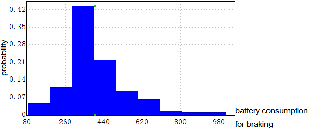
(a) Histogram of probability distribution of energy estimation

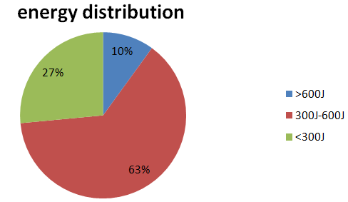
(b) Pie chart of probability

Figure 6.8: Energy estimation of braking mode

6.3 Simulink & Stateflow  Simulation using Matlab  tool

In our experiments, simulation is conducted in Simulink and Uppaal-smc to validate both functional properties and the non-functional properties.

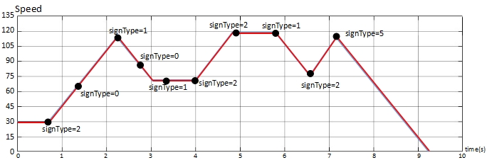
Figure 6.9: The simulation result of maximum and minimum speed limit in S/S model

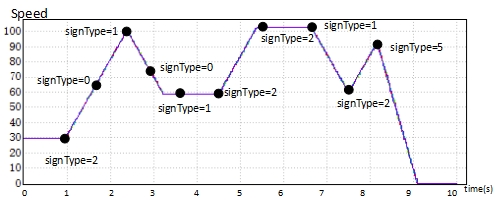
Figure 6.10: The simulation result of maximum and minimum speed limit in Uppaal-smc model

In this chapter, we present several simulation results of the requirements on the vehicle. For example, as shown in Fig.6.9, the requirements of R8, R10-R15, R18, R19, R24, R25, and R32-R34 are validated. When time equals to 0.61s and a minimum speed limit sign (signType == 2) is detected, since the current speed of the vehicle is 30m/s (less than min_speed_limit 70), the speed of the vehicle is increased. Thus R10 is validated. During the acceleration, a straight sign is recognized, and the vehicle keeps accelerating, which satisfies R18. At 2.2s, the vehicle recognizes a maximum speed limit sign (signType == 1 and the speed_limit is 100), it then decreases its speed. R14 is then guaranteed. Afterwards, the vehicle detects a straight sign, it continues decelerating its speed. In this case, R19 is satisfied. After completing the deceleration, the vehicle maintains the speed. At 3.4s, a maximum speed limit sign (100) is recognised, because the current speed of the vehicle is less than 100 according to R15, the speed of the vehicle is unchanged until 4s, at which the vehicle detects a minimum speed limit sign (80). The vehicle increases its speed to 119m/s. Then a minimum speed limit sign appears again, but as the speed of the vehicle now is 119, larger than min_speed_limit 70, the vehicle will keep its speed as R13. At 5.76s, a maximum speed limit sign is recognised, and the vehicle decreases its speed to satisfy the max_speed_limit which is 100, which satisfies R11. During the deceleration, if a minimum speed limit sign 80 is recognised and the speed of the vehicle is lower than 80, the vehicle will increase its speed according to R12. Finally, at 7.1s during acceleration, a stop sign is recognised, so the vehicle decreases the speed of its four wheels till 0, which validates R8. According to Fig.6.9, the longest acceleration time is 1.59s and the longest deceleration time is 0.82s, thus R32 and R33 is proved. The deceleration time for stop is 2.06s, satisfying R34. The differences between the speeds of the (front and rear) wheels on the left and right are nearly 0, as the four lines representing speed are almost overlapped. Similarly, the speeds of the four wheels are shown, and the requirements mentioned above can be proved from Fig.6.10.

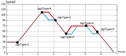
Figure 6.11: The simulation result of turning left in S/S model

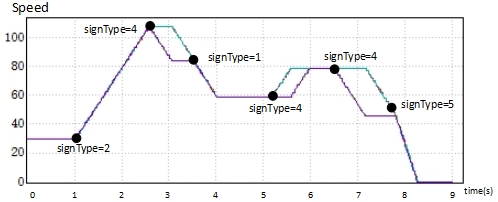
Figure 6.12: The simulation result of turning left in Uppaal-smc model

In Fig.6.11, R1-3, R16, R20-R21, R30 and R35 can be validated. At 0.64s, a minimum speed limit sign (signType == 2) is recognised, and as the speed of the vehicle now is 30m/s, which is less than the min_speed_limit 80, so the vehicle will increase its speed. During the acceleration, at 2.23s, a turn_left sign (signType == 4) is recognised. As the speed of the vehicle now is 112, larger than 70 (high speed), so the vehicle will decrease the speeds of rear and front left wheels to turn left, which satisfies R2 and R20. At 3.78s, as the speed of the vehicle is 52, less than 70 (low speed), the vehicle will turn left as a turn_left sign is recognised. This time, the turning is realized by increasing speeds of rear and front right wheels, according to R3 and R21. After the vehicle turns left, the vehicle will run at a constant speed, when at 5.05s, a turn_left sign is recognised. So the vehicle will turn left, which validates R1. During the turning, at 5.69s, a stop sign is recognised. The vehicle will finish turning, and then decrease to stop. Thus R16 is validated. Finally, the vehicle will stop with all the speed of the four wheels equals to 0, thus validates R24. The turning time are 0.906s, 0.8s and 0.91s, within 0.8s to 1.5s, thus R35 is validated. Similarly, the behaviour of the vehicle’s turning can be seen from Fig.6.12, and the requirements can be validated from differences among speeds. The vehicle will turn left by either increasing speed of the right wheels or decreasing speed of the left wheels depends on the speed of the vehicle, and the turning time is within [0.8s,1.5s], thus the requirements R30 and R35 can be valid.

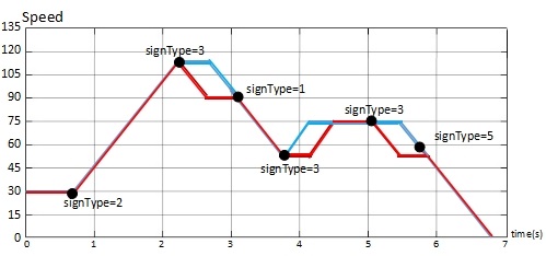
Figure 6.13: The simulation result of turning right in S/S model

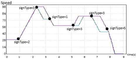
Figure 6.14: The simulation result of turning right in Uppaal-smc model

In Fig.6.13, R4-6, R17, R22-R23, R31 and R36 can be validated. At 0.62s, a minimum speed limit sign (signType == 2) is recognised, and as the speed of the vehicle now is 30m/s, which is less than the min_speed_limit 70, so the vehicle will increase its speed. During the acceleration, at 2.2s, a turn_right sign (signType == 3) is recognised. As the speed of the vehicle now is 110, larger than 70 (high speed), so the vehicle will decrease the speeds of rear and front right wheels to turn right, which satisfies R5 and R22. At 3.76s, when the vehicle is decelerating, it recognised a turn right sign. Thus it turn left, which satisfies R6. As the speed of the vehicle is 55, less than 70 (low speed), the vehicle will turn right as a turn_right sign is recognised. This time, the turning is realized by increasing speeds of rear and front left wheels according to R23. After the vehicle turns right, the vehicle will run at a constant speed, when at 5.0s, a turn_right sign is recognised. So the vehicle will turn right according to R4. During the turning, at 5.72s, a stop sign is recognised. The vehicle will finish turning, and then decrease to stop. Thus R17 can be validated. Finally, the vehicle will stop with all the speed of the four wheels equals to 0, thus validates R24. The turning time are 0.91s, 0.82s and 0.915s, within 0.8s to 1.5s, thus R36 is validated. During the whole run of the vehicle, when it is turning right, the speed of the left wheels are always no less then that of the right wheels. Thus R31 is valid. Recall Fig.6.14, same requirements can be valid in Uppaal-smc model.

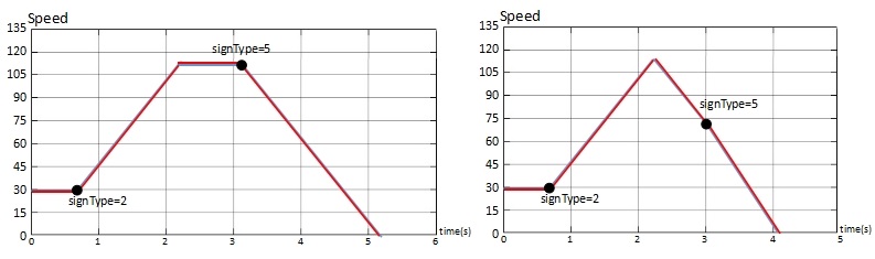
Figure 6.15: The simulation result of stop

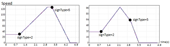
Figure 6.16: The simulation result of stop

In Fig.6.15, R7 and R9 can be validated. No matter whether the vehicle is driving at a constant speed, or the vehicle is decreasing its speed, if a stop sign is detected, the vehicle will decrease its speed and stop at last. Same requirements can also be valid from Fig.6.16, as whenever the vehicle recognises a stop sign, the vehicle will decrease its speed to stop.

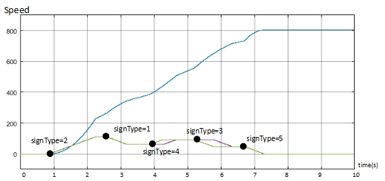
Figure 6.17: The simulation result of energy consumption

How the energy consumption rate of Controller changes and how the estimated energy consumption is influenced by the change are monitored using Simulink
(Fig.6.17) and Uppaal-smc (Fig.6.18). In Fig.6.17, AV detects the minimum speed limit sign (signType = 2) and it increases its speed (green and red curve). Since energy rate is proportional to speed, the energy consumption (blue curve) is continuously raised until AV detects the maximum speed limit sign (signType = 1). AV slows down after it reaches the maximum speed at 3.2s leading to a slow decrease in energy consumption accordingly. Then a turn left sign is recognised, thus the vehicle increases the speed of its right wheels, and then turn right due to a turn right sign. Energy consumption increases faster than in constSpeed mode. Then a stop sign is recognised at 6.6s, the energy consumption of the vehicle increases with a rapid increase rate. The energy consumption for each movement of the vehicle are: 223J (acceleration), 138J (deceleration), 125J (left turn), 150J (right turn) and 80J (stop). Thus R40-R45 can be validated. In Fig.6.18, same behaviour of the AV can be seen, and according energy consumption can be proved.

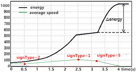
Figure 6.18: Energy Consumption Estimation in Uppaal-smc

Fig.6.19 illustrates the simulation results of execution constraints (R46, R47) in Simulink and in Uppaal-smc: In the upper graph (Fig.6.19.(a)), Camera consumes energy within 100ms (red line), which demonstrates R46. is valid. In the lower graph, the time between the occurrences whereby Sign Recognition receives a detected image from Camera and sends out its corresponding sign type (blue line) to Controller is within [200ms,600ms] thus validating R46. Similarly, in the simulation of Uppaal-smc (Fig.6.19.(b)), the execution times of Camera (green line) and Sign Recognition (distance between green and red lines) satisfy R47 and R46 respectively.

Furthermore, 1. Cameracaptures an image almost every 700ms with a deviation of 100ms; 2. The time intervals among different images Camera captured are within 700ms with the deviation 100ms . Both are illustrated in Fig.6.19.(a). Therefore, Periodic constraint (R49) is established as valid.

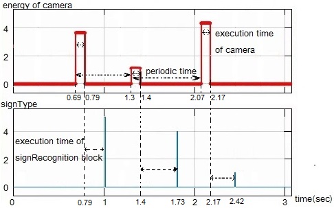
(a) Simulation in Simulink

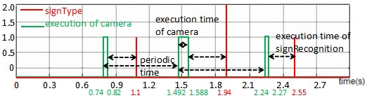
(b) Simulation in Uppaal-smc

Figure 6.19: Simulation of Execution and Periodic Constraints

Fig.6.20(a) demonstrates Synchronization constraint (R48) is valid: The blue line denotes the time point of which Controller detects a sign type. The other lines (represented by four different colors) indicate the time points of which Controller recognizes the speed signals of the four wheels. In both Fig.6.20(a).(a) and (b), the earliest event arrival time and the lastest event arrival time among all input events are within the 400ms tolerance.

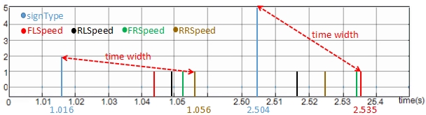
(a) Simulation in Simulink

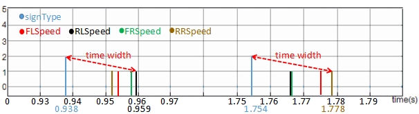
(b) Simulation in Uppaal-smc

Figure 6.20: Simulation of Synchronization Constraint

Fig.6.21 illustrates the simulation result of end-to-end constraint (R50) in Uppaal-smc: The red (blue) line indicates whether Camera (SignRecognition) is executed or not. The time between Sign Recognition receives a detected image from Camera (red line) and sends out its corresponding sign type (blue line) to Controller is within [200ms, 600ms] thus validating R50. Recall Fig.6.19.(a), R50 is similarly valid in Simulink.

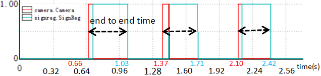
Figure 6.21: Simulation of End-to-End constraint in Uppaal-smc

Chapter 7 Related work

In the context of East-adl, an effort on the integration of East-adl and formal techniques based on timing constraints was investigated in several works [21, 22, 23], which are however, limited to the executional aspects of system functions without addressing energy-aware behaviors. An earlier study [24, 25] was performed towards the formal analysis of energy-aware East-adl models based on informal semantics of East-adl architectural models. Kang [9], Goknil et al. [26] and Seceleanu et al. [27] defined the execution semantics of both the controller and the environment of industrial systems in Ccsl [28] which are also given as mapping to Uppaal models amenable to model checking. In contrast to our current work, those approaches lack precise stochastic annotations specifying continuous dynamics in particular regarding different energy consumption rates during execution. Though, Kang et al. [11, 10] and Marinescu et al. [29] present both simulation and model checking approaches of Simulink and Uppaal-smc on East-adl models, neither formal specification nor verification of extended East-adl timing constraints with probability were conducted. Our approach is a first application on the integration of East-adl and formal V&V techniques based on a composition of energy- and probabilistic extension of East-adl/Tadl constraints.

There are several works that discuss formal analysis approaches to verify the requirements of the system model. Integrated in the Simulink environment, SDV is a powerful tool for verifying the property of Simulink/Stateflow model. In [30], Ali etc. compared Uppaal-smc and SDV for usability and adaptability for the functional requirements. In our work, applicability of SDV is evaluated by adding a set of non-functional properties. We translate Simulink/Stateflow model to Uppaal-smc and make advantages of Uppaal-smc  to verify the non-functional properties, which to some extent helps make up the limitation for expressing non-functional properties of SDV. Leitner[31] compares SDV with SPIN and concludes that SDV can only prove the properties written as assertions, but SPIN can also check the temporal properties. In our work, we found that not only assertions can be checked in SDV of MATLAB2014b, but also functionally temporal property can be verified. What’s more, we use Uppaal-smc instead of SPIN as there are some stochastic events in our plant, and we verify probabilistic timing constraints of our system to reduce the consumed time of verification. Filipovikj et al. [32] focus on the verification of Simulink blocks and proposed a method to transform Simulink blocks to Uppaal SMC model, which is limited in tackling timing requirements. In contrast to our work, we translate Simlink/Stateflow model and propose method for timing constraints analysis in Uppaal SMC. Moreover, simulation in both Simulink/Stateflow model and Uppaal model are conducted to ensure the consistency of the translation.

Chapter 8 Conclusion

We present an approach to perform non-functional properties verification and support stochastic analysis of an autonomous vehicle system at the early design phase: 1. East-adl/Tadl2 are used for structural, timing- and $f_{p}$’s causality constraints; the execution semantics of timing- and energy constraints are visualized in Simulink and specified in Uppaal-smc; 2. probabilistic extension of East-adl constraints is defined and the semantics of the extended constraints is translated into verifiable Uppaal-smc models with stochastic semantics for formal verification; 3. A set of mapping rules is proposed to facilitate the guarantee of translation. Simulation and V&V are performed on the extended timing and energy constraints using Uppaal-smc and Simulink; 4. The applicability of our approach in an autonomous automotive product is demonstrated.

We discuss open issues: 1. Although we have shown that our approach preserves ERT behaviors and the probabilistic extension of timing constraints of the AV model and that the obtained Uppaal-smc and Simulink models manifest the same behaviors and constraints, there is no formal correctness proof for the derived procedures. As ongoing work, we use conformance checking to show that the translation procedure correctly preserves probabilistic ERT behaviors and constraints; 2. From the tooling perspective, a dedicated plugin that directly provides translation of Simulink/Stateflow to Uppaal-smc in fully automatic will supplement our tool chain, A-BeTA (A$\beta$: EAST-ADL Behavioral Modeling and Translation into Aanalyzable Model) [25, 9, 8] for both model checking and simulation. We formally prove the validity of the obtained Uppaal-smc

References

- [1] “ISO 26262-6: Road vehicles functional safety part 6. Product development at the software level. international organization for standardization, geneva,” 2011.
- [2] “IEC 61508: Functional safety of electrical/electronic/programmable electronic safety related systems. international organization for standardization, geneva,” 2010.
- [3] A. David, D. Du, K. G. Larsen, A. Legay, M. Mikucionis, D. B. Poulsen, and S. Sedwards, “Statistical model checking for stochastic hybrid systems,” in HSB, ser. EPTCS 92, 2012, pp. 122–136.
- [4] A. David, K. G. Larsen, A. Legay, M. Miku cionis, and D. B. Poulsen, “UPPAAL-SMC Tutorial,” International Journal on Software Tools for Technology Transfer, vol. 17, no. 4, pp. 397–415, 2015.
- [5] EAST-ADL Consortium, “East-adl domain model specification v2.1.9,” Maenad European Project, Tech. Rep., 2011. [Online]. Available: www.maenad.eu/public/EAST-ADL-Specification_M2.1.9.1.pdf
- [6] “Simulink and StateFlow,” http://www.mathworks.nl/products/.
- [7] H. Blom, L. Feng, H. Lönn, J. Nordlander, S. Kuntz, B. Lisper, S. Quinton, M. Hanke, M.-A. Peraldi-Frati, A. Goknil, J. Deantoni, G. B. Defo, K. Klobedanz, M. zhan, and O. Honcharova, “Timing Model, Tools, algorithms, languages, methodology, USE cases,” TIMMO-2-USE, Tech. Rep., 2012.
- [8] E. Kang, G. Perrouin, and P. Schobbens, “Towards formal energy and time aware behaviors in east-adl: An mde approach,” in QSIC12. IEEE, 2012, pp. 124–127.
- [9] E. Kang and P. Schobbens, “Schedulability analysis support for automotive systems: from requirement to implementation,” in Symposium on Applied Computing, SAC 2014, Gyeongju, Republic of Korea - March 24 - 28, 2014, 2014, pp. 1080–1085.
- [10] E. Kang, L. Ke, M. Hua, and Y. Wang, “Verifying automotive systems in east-adl/stateflow using UPPAAL,” in 2015 Asia-Pacific Software Engineering Conference, APSEC 2015, New Delhi, India, December 1-4, 2015. IEEE, 2015, pp. 143–150.
- [11] E. Kang, J. Chen, L. Ke, and S. Chen, “Statistical analysis of energy-aware real-time automotive systems in east-adl/stateflow,” in 11th International Conference on Industrial Electronics and Applications (ICIEA). IEEE, 2016, pp. 1328–1333.
- [12] “UPPAAL Tools,” http://www.uppaal.org.
- [13] “UPPAAL-SMC,” http://people.cs.aau.dk/~adavid/smc/.
- [14] “Simulink Design Verifier,” https://www.mathworks.com/products/sldesignverifier/.
- [15] “what is sample time,” https://cn.mathworks.com/help/simulink/ug/what-is-sample-time.html, 2016.
- [16] R. Alur and D. L. Dill, “A theory of timed automata,” Theoretical Computer Science, vol. 126, no. 2, pp. 183–235, 1994.
- [17] “YCbCr definition and convert,” https://www.mathworks.com/help/images/convert-from-ycbcr-to-rgb-color-space.html.
- [18] MetaCase, http://www.metacase.com/mep/, 2017.
- [19] Mathworks, “Simulink model of traffic warning sign recognition,” https://www.mathworks.com/examples/simulink-computer-vision/mw/vision_product-vipwarningsigns-traffic-warning-sign-recognition.
- [20] E.-Y. Kang, J. Chen, L. Ke, and S. Chen, “Statistical analysis of energy-aware real-time automotive systems in east-adl/stateflow,” in Industrial Electronics and Applications (ICIEA), 2016 IEEE 11th Conference on. IEEE, 2016, pp. 1328–1333.
- [21] T. Naseer Qureshi, D. Chen, M. Persson, and M. Törngren, “Towards the integration of uppaal for formal verification of east-adl timing constraint specification,” in TiMoBD workshop, 2011.
- [22] E. Kang, E. P. Enois, R. Marinescu, C. Seceleanu, P. Schobbens, and P. Pettersson, “A methodology for formal analysis and verification of EAST-ADL models,” Reliability Engineering and System Safety Journal, pp. 127 – 138, 2013.
- [23] E. Kang, P. Schobbens, and P. Pettersson, “Verifying functional behaviors of automotive products in EAST-ADL2 using UPPAAL-PORT,” in SAFECOMP. Springer LNCS, vol 6894, September 2011, pp. 243–256.
- [24] E. Kang and P. Schobbens, “Extending east-adl towards formal modeling and analysis of energy-aware real-time systems,” in ICCA13. IEEE, 2013, pp. 1890–1895.
- [25] E. Kang, G. Perrouin, and P. Schobbens, “Model-based verification of energy-aware real-time automotive system,” in ICECCS13. IEEE Computer Society, 2013, pp. 135 – 144.
- [26] A. Goknil, J. Suryadevara, M.-A. Peraldi-Frati, and F. Mallet, “Analysis support for tadl2 timing constraints on east-adl models,” Software Architecture: 7th European Conference, ECSA, 2013.
- [27] C. Seceleanu, M. Johansson, J. Suryadevara, G. Sapienza, T. Seceleanu, S.-E. Ellevseth, and P. Pettersson, “Analyzing a wind turbine system: From simulation to formal verification,” Science of Computer Programming, vol. 133, pp. 216–242, 2017.
- [28] F. Mallet, M.-A. Peraldi-Frati, and C. Andre, “MARTE CCSL to execute east-adl timing requirements,” in ISORC ’09, 2009, pp. 249 –253.
- [29] R. Marinescu, H. Kaijser, M. Mikuèionis, C. Seceleanu, H. Lönn, and A. David, “Analyzing industrial architectural models by simulation and model-checking,” in Third International Workshop on Formal Techniques for Safety-Critical Systems, November 2014.
- [30] S. Ali, M. Sulyman, M. Nyberg, J. Westman, G. Dellapenna, G. R.-N. González, and P. Pettersson, “Applying model checking for verifying the functional requirements of a scania s vehicle control system,” 2012.
- [31] F. Leitner-Fischer and S. Leue, “Simulink design verifier vs. spin: a comparative case study,” 2008.
- [32] P. Filipovikj, N. Mahmud, R. Marinescu, C. Seceleanu, O. Ljungkrantz, and H. Lönn, “Simulink to uppaal statistical model checker: Analyzing automotive industrial systems,” in FM 2016: Formal Methods: 21st International Symposium, Limassol, Cyprus, November 9-11, 2016, Proceedings 21. Springer, 2016, pp. 748–756.