Expected Time to Extinction of SIS Epidemic Model Using Quasy– Stationary Distribution

Abstract

We study that the breakdown of epidemic depends on some parameters, that is expressed in epidemic reproduction ratio number. It is noted that when $R_{0}$ exceeds 1, the stochastic model have two different results. But, eventually the extinction will be reached even though the major epidemic occurs. The question is how long this process will reach extinction. In this paper, we will focus on the Markovian process of SIS model when major epidemic occurs. Using the approximation of quasi–stationary distribution, the expected mean time of extinction only occurs when the process is one step away from being extinct. Combining the theorm from Ethier and Kurtz, we use CLT to find the approximation of this quasi distribution and successfully determine the asymptotic mean time to extinction of SIS model without demography.

1 Introduction

According to the threshold theorem, epidemic can only occur if the initial number of susceptibles is larger than some critical values, which depends on the parameters under cosideration [4] . Usually, it is expressed in terms of epidemic reproductive ratio number, $R_{0}$.

Susvitasari [22] showed that both deterministic and stochastic models performed similar results when $R_{0}\leq 1$, i.e. the disease–free stage in the epidemic. But then, when $R_{0}>1$, the deterministic and stochastic models had different interpretations. In the deterministic model, both SIS and SIR showed an outbreak of the disease, and after some time $t$, the disease persisted and reached equilibrium stage, i.e. endemic. The stochastic model, on the other hand, had different interpretation. There are two possible outcomes of this approach. First, the infection may die out in the first cycle. If it did, it would happen very quickly since the time of the disease removed must less than the time of infectee–susceptible contact. Second, if it survives the first cycle, the outbreak was likely to occur, but after some time $t$, it would reach equilibrium as the deterministic version. In fact, the stochastic model would mimic the deterministic path and scattered randomly around its equilibrium. Furthermore, by letting population size be large and ignoring the initial value of infectious individuals, as $t\rightarrow\infty$, the empirical distribution of $n^{-1}Y_{n}(t)$, where $Y_{n}(t)$ is the number of infectious individuals at time $t$ with $n$ population size followed normal distribution in endemic phase as seen in Figure 2.

In this paper, we will focus on the endemic stage, the stage where $R_{0}>1$ and the outbreak occurs in SIS epidemic model without demography to determine the expected mean time to extinction of this model.

2 The Birth and Death Process in SIS

Suppose that $\{Y_{n}(t):t\geq 0\}$ denotes the Markovian process that represents the number of infected individuals in the population at time $t$. Then we define $S_{n}=\{0,1,\ldots,n\}$ as the state space of the process, where state zero is an absorbing state. Figure 1 is the illustration of this process.

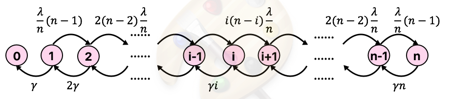
Figure 1: Birth–death of SIS without demography transition process

Consider the case where $R_{0}>1$ and the outbreak occurs. Eventually, given a necessary large $n$ and some time $t$, the process will not visit state zero. So, let us redefine the birth–death process before by only considering the transient states. Let $\{\hat{Y}_{n}(t):t\geq 0\}$ be the modified process of $\{Y_{n}(t):t\geq 0\}$ with state space $S_{n}^{\prime}=S_{n}\setminus\{0\}$. The intuitive explaination is that whenever the SIS process goes extinct, it immediately will restart again in state 1. It is not hard to show that the process $\{\hat{Y}_{n}(t):t\geq 0\}$ is time–reversible Markov chain. Therefore, there exist colections of equilibrium distributions $\pi_{j}$ for all $j\in S_{n}^{\prime}$ that sums to unity and satisfy the detailed–balanced conditions:

1. $(n-1)\displaystyle\frac{\lambda}{n}\hat{\pi}_{i}=2\gamma\hat{\pi}_{2}$,

2. $\left(i(n-i)\displaystyle\frac{\lambda}{n}+\gamma i\right)\hat{\pi}_{i}=(i-1)(n-i+1)\displaystyle\frac{\lambda}{n}\hat{\pi}_{i-1}+(i+1)\gamma\hat{\pi}_{i+1}$   $i=2,3,\ldots,n-1$,

3. $n\gamma\hat{\pi}_{n}=(n-1)\displaystyle\frac{\lambda}{n}\hat{\pi}_{n-1}$,

with constraint $\displaystyle\sum_{i\in S_{n}^{\prime}}\hat{\pi}_{i}=1$. Thus the solution is

$$\hat{\pi}_{i}=\frac{1}{i}\left(\frac{\lambda}{n\gamma}\right)^{i-1}\frac{(n-1)!}{(n-i)!}\hat{\pi}_{1}\qquad i=1,2,\ldots,n.$$ (1)

Therefore,

$$\hat{\pi}_{1}=\left(\sum_{i=1}^{n}\frac{(n-1)!}{i(n-i)!}\left(\frac{\lambda}{n\gamma}\right)^{i-1}\right)^{-1}.$$ (2)

Now, let $T_{ext}^{(n)}$ denote the time to extinction in SIS epidemic model. Recall that the process $\{\hat{Y}_{n}(t):t\geq 0\}$ is time-reversible on state $S_{n}^{\prime}$. Then, the time to extinction $T_{ext}^{(n)}$ is almost surely finite since the state $S_{n}^{\prime}$ is visited finitely often.

Suppose that $\{\hat{Y}_{n}(t):t\geq 0\}$ is in equilibrium, then the mean time to extinction has intensity $\hat{\pi}_{1}$ times the rate of the process getting absorbed to state $\{0\}$.

$$E\left(T_{ext}^{(n)}\right) =E(\text{interarival time of jump }1\rightarrow 0)$$

$$=\frac{1}{\gamma\hat{\pi}_{1}}=\frac{1}{\gamma}\sum_{i=1}^{n}\frac{(n-1)!}{i(n-i)!}\left(\frac{\lambda}{n\gamma}\right)^{i-1}.$$ (3)

As $n\rightarrow\infty,E\left(T_{ext}^{(n)}\right)\rightarrow\displaystyle-\frac{\log{(1-\lambda)}}{\lambda}$ when we set $R_{0}<1$. Ball et al. [6] showed the approximation of mean time extinction when $R_{0}<1,R_{0}=1,$ and $R_{0}>1$.

In this paper, we will focus on the time to extinction when the process reaches endemic–stage, i.e. when $R_{0}>1$ and the process survives the first cycle of extinction using quasi– statioary distribution and property of central limit theorm.

3 Expected Time of Extinction of SIS in Endemic–Stage

Before we start this section, we will introduce first the quasi–stationary distribution.

3.1 Quasi–Stationary Distribution

Recall the process $\{Y_{n}(t):t\geq 0\}$ with finite state space $S_{n}$, where 0 is an absorbing state. For $j\in T=S_{n}\setminus\{0\}$, let

$$q_{i,j}(t) =P(Y_{n}(t)=j\mid Y_{n}(t)>0,Y_{n}(0)=i)$$

$$=\frac{P_{i,j}(t)}{1-P_{i,0}(t)}\qquad i=1,2,\ldots,n.$$ (4)

Since we concerns on the distribution of the process in endemic stage, we wish to find $\tilde{q}_{j}=\displaystyle\lim_{t\rightarrow\infty}q_{i,j}(t)$.

We define $A$ and $T$ as sets of absorbing and transient state. Suppose

$$\boldsymbol{Q}=\left[\begin{array}[]{cc}\boldsymbol{Q}_{AA}&\boldsymbol{0}\\ \boldsymbol{Q}_{TA}&\boldsymbol{Q}_{TT}\end{array}\right]$$

where $\boldsymbol{Q}$ is transition rate matrix, defined as $\boldsymbol{Q}=(q_{ij})_{i,j\in S_{n}}$. Let $\boldsymbol{W}=diag_{n\times n}(\boldsymbol{\hat{\pi}})$. Since $\boldsymbol{W}^{1/2}\boldsymbol{Q}_{TT}\boldsymbol{W}^{-1/2}$ is symmetry, according to spectral decomposition theorem,

$$\boldsymbol{W}^{1/2}\boldsymbol{Q}_{TT}\boldsymbol{W}^{-1/2}=\sum_{i=1}^{n}\lambda_{i}\boldsymbol{u}_{i}\boldsymbol{u}_{i}^{T},$$

where $\lambda_{1},\lambda_{2},\ldots,\lambda_{n}$ are eigenvalues of $\boldsymbol{W}^{1/2}\boldsymbol{Q}_{TT}\boldsymbol{W}^{-1/2}$ and $\boldsymbol{u}_{1},\boldsymbol{u}_{2},\ldots,\boldsymbol{u}_{n}$ are corresponding orthonormal vectors of right-eigenvectors. Therefore,

$$\boldsymbol{Q}_{TT}=\sum_{i=1}^{n}\lambda_{i}\boldsymbol{E}_{i}\Rightarrow\boldsymbol{Q}_{TT}\cdot t=\sum_{i=1}^{n}\lambda_{i}t\cdot\boldsymbol{E}_{i}\Rightarrow exp(\boldsymbol{Q}_{TT}t)=exp\left(\sum_{i=1}^{n}\lambda_{i}t\cdot\boldsymbol{E}_{i}\right),$$ (5)

where $\mathbb{E}_{i}=\left(\mathbb{W}^{-1/2}\mathbb{u}_{i}\right)\left(\mathbb{u}_{i}^{T}\mathbb{W}^{1/2}\right)$ and we can see in Appendix ……… that $exp(\boldsymbol{Q}_{TT}t)=\displaystyle\sum_{i=1}^{n}exp(\lambda_{i}t)\boldsymbol{E}_{i}$. Recall that forward Kolmogorov equation, $\mathbb{P}(t)$ must satisfy $\mathbb{P}^{\prime}(t)=\mathbb{P}(t)\mathbb{Q}$, where $\mathbb{P}(0)=\mathbb{I}_{n\times n}$ with solution $\mathbb{P}(t)=exp(\mathbb{Q}t)$. So, for $i,j\in T$,

$$P_{i,j}(t) =P\{Y_{n}(t)=j\mid Y_{n}(0)=i\}$$

$$=\left[e^{\boldsymbol{Q}_{TT}t}\right]_{ij}=\left[\sum_{k=1}^{n}e^{\lambda_{k}t}\boldsymbol{E}_{k}\right]_{ij}.$$ (6)

According to Darroch and Seneta [12] there exists a simple, real eigenvalue $\lambda_{1}<0$ such that all other eigenvalues of $\boldsymbol{W}^{1/2}\boldsymbol{Q}_{TT}\boldsymbol{W}^{-1/2}$ have real part less than $\lambda_{1}$. Therefore, eq. (4) becomes

$$q_{i,j}(t) =\frac{\displaystyle e^{\lambda_{1}t}(\boldsymbol{E}_{1})_{ij}+e^{\lambda_{2}t}(\boldsymbol{E}_{2})_{ij}+\ldots+e^{\lambda_{n}t}(\boldsymbol{E}_{n})_{ij}}{\displaystyle\sum_{l=1}^{n}\{e^{\lambda_{1}t}(\boldsymbol{E}_{1})_{il}+e^{\lambda_{2}t}(\boldsymbol{E}_{2})_{il}+\ldots+e^{\lambda_{n}t}(\boldsymbol{E}_{n})_{il}\}}$$

$$=\frac{\displaystyle(\boldsymbol{E}_{1})_{ij}+e^{(\lambda_{2}-\lambda_{1})t}(\boldsymbol{E}_{2})_{ij}+\ldots+e^{(\lambda_{n}-\lambda_{1})t}(\boldsymbol{E}_{n})_{ij}}{\displaystyle\sum_{l=1}^{n}\{(\boldsymbol{E}_{1})_{il}+e^{(\lambda_{2}-\lambda_{1})t}(\boldsymbol{E}_{2})_{il}+\ldots+e^{(\lambda_{n}-\lambda_{1})t}(\boldsymbol{E}_{n})_{il}\}}.$$ (7)

Consequently, as $t\rightarrow\infty,\tilde{q}_{j}=\displaystyle\frac{(\mathbb{E}_{1})_{ij}}{\sum_{l=1}^{n}(\mathbb{E}_{1})_{il}}$.

Note that $\boldsymbol{E}_{1}=\left(\boldsymbol{W}^{-1/2}\boldsymbol{u}_{1}\right)\left(\boldsymbol{u}_{1}^{T}\boldsymbol{W}^{1/2}\right)$ and it turns out that $\left(\boldsymbol{u}_{1}^{T}\boldsymbol{W}^{1/2}\right)$ is left eigenvector of $\boldsymbol{Q}_{TT}$ (see Appendix B). In the stationary scenario, when $t\rightarrow\infty$, each row of probability transition matrix $\boldsymbol{P}(t)$ has nearly similar entries. So, it follows that the quasi-distribution $\tilde{\boldsymbol{q}}$ is given by the left-eigenvector of $\boldsymbol{Q}_{TT}$ corresponding to eigenvalue $\lambda_{1}$ with constraint $\tilde{\boldsymbol{q}}\boldsymbol{1}=\displaystyle\sum_{k=1}^{n}\tilde{q}_{k}=1$.

3.2 Expected Time to Extinction by Quasi–Stationary Distribution

Suppose that $\left(Y_{n}(t)\mid Y_{n}(t)>0,Y_{n}(0)=i\sim\tilde{\boldsymbol{q}}\right)$ and let $T_{Q}=\inf{\{t\geq 0;Y_{n}(t)=0,Y_{n}(t)\sim\tilde{\boldsymbol{q}}}\}$. Since two events (infection and recovery) in the epidemic model follows the Poisson process, there is zero probability that two or more events occur at the same time. So, the extinction only occurs when the process is one step away from being extinct. Therefore,

$$P(\text{not extinct at time }t) =P\left(T_{Q}>t\right)$$

$$=\sum_{j=1}^{n}\lim_{t\rightarrow\infty}P(Y_{n}(t)=j\mid Y_{n}(0)=i)$$

$$=\sum_{j=1}^{n}\tilde{q}_{j}\cdot P(Y_{n}(t)>0)$$

$$=\sum_{j=1}^{n}\tilde{q}_{j}\cdot e^{\boldsymbol{Q}_{TT}t}=\tilde{\boldsymbol{q}}\cdot e^{\boldsymbol{Q}_{TT}t}\cdot\boldsymbol{1}.$$ (8)

Recall that $\tilde{\boldsymbol{q}}$ is the left-eigenvector of $\boldsymbol{Q}_{TT}$, corresponding to the eigenvalue $\lambda_{1}$. So,

$$\tilde{\boldsymbol{q}}\cdot\boldsymbol{Q}_{TT}=\lambda_{1}\tilde{\boldsymbol{q}}\quad\Rightarrow\quad\tilde{\boldsymbol{q}}\cdot\boldsymbol{Q}_{TT}^{k}=\lambda_{1}^{k}\tilde{\boldsymbol{q}}\quad\Rightarrow\quad\tilde{\boldsymbol{q}}\cdot e^{\boldsymbol{Q}_{TT}t}=e^{\lambda_{1}t}\tilde{\boldsymbol{q}}.$$

Hence, the equation (8) becomes

$$P(\text{not extinct at time }t) =e^{\lambda_{1}t}.$$ (9)

Since the process is Poisson process, then the inter arrival time must follow exponential distribution. Therefore, in eq. (9), $T_{Q}$ follows exponential distribustion with intensity $-\lambda_{1}$. But, recall the memoryless property of the Poisson process and that the extinction only occurs if the process is one step away from being extinct. Intuitively, it also means that the extinction happens with intensity $\tilde{q}_{1}$ times the rate of the process to jump into absorption state $0$, which is $\gamma$. On the other hand, $\lambda_{1}=-\gamma\tilde{q}_{1}$ (note that $\lambda_{1}<0$).

Proof.

Using the fact that $\tilde{\boldsymbol{q}}$ is the left-eigenvector of $\boldsymbol{Q}_{TT}$,

$$\tilde{\boldsymbol{q}}\cdot\boldsymbol{Q}_{TT}=\lambda_{1}\tilde{\boldsymbol{q}}\Rightarrow\tilde{\boldsymbol{q}}\cdot\underbrace{\boldsymbol{Q}_{TT}\cdot\boldsymbol{1}}_{(-\gamma,0,\ldots,0)^{T}}=\lambda_{1}\underbrace{(\tilde{\boldsymbol{q}}\boldsymbol{1})}_{=1}\Rightarrow-\gamma\cdot\tilde{q}_{1}=\lambda_{1}.$$

∎

Therefore, the mean time to extinction of the SIS process is

$$E\left(T_{Q}\right) =\frac{1}{\gamma\tilde{q}_{1}}.$$ (10)

where $\tilde{q}_{1}=(\tilde{\boldsymbol{q}})_{1}$.

The quasi–stationary is a very powerful approximation when we let population size large enough. Unfortunately, consider that by using this method, we need to capture all the possible transition rate for matrix $\mathbb{Q}$. Considering the large $n$, the size of matrix $\mathbb{Q}$ will also big and leads to inefficient computation. Therefore, we should approximate the distribution of $\tilde{q}_{1}$.

Now, suppose that we only concern on the size of infectious individuals in population when the outbreak occurs, i.e. $\{Y_{n}(t)|Y_{n}(t)>0,Y_{n}(t)\sim\mathbb{\tilde{q}}\}$. By ignoring the initial value of infectives, the empirical distribution of $n^{-1}Y_{n}(t)$ follows normal distribution with mean converges to equilibrium point in deterministic model as seen in Figure 2. It turns out that by applying Central Limit Theorem, we could approximate the quantity of $\tilde{q}_{1}$.

4 Central Limit Theorem

We define $\{\boldsymbol{X}_{n}(t);t\geq 0\}$ to be the CTMC on $\mathbb{Z}^{d}$ with finite state space and finite number of possible transition $\boldsymbol{l}\in\Delta\subseteq\mathbb{Z}^{d}$ in such a way that $\beta_{\boldsymbol{l}}:\mathbb{Z}^{d}\rightarrow[0,\infty),\sum_{l\in\Delta}\beta_{l}(\boldsymbol{x})<\infty$ for all $\boldsymbol{x}\in\mathbb{Z}^{d}$. Then let $F(\boldsymbol{x})=\sum_{\boldsymbol{l}\in\Delta}\boldsymbol{l}\beta_{\boldsymbol{l}}(\boldsymbol{x})$ as the drift function of the process $\{\boldsymbol{X}_{n}(t):t\geq 0\}$.

Suppose that $F(\boldsymbol{x})$ is a continuous function and differentiable in $\mathbb{Z}^{d}$ lattice such that $\partial F(\boldsymbol{x})$ exists and is continuous and let $G(\boldsymbol{x})$ be $d\times d$ matrix function defined as

$$G(\boldsymbol{x})=\displaystyle\sum_{\boldsymbol{l}\in\Delta}\boldsymbol{l}^{T}\boldsymbol{l}\beta_{\boldsymbol{l}}(\boldsymbol{x}).$$

Further, let $\Phi(t,s)$, where $0\leq s\leq t$, be the solution of the matrix differential equation

$$\frac{\partial}{\partial t}\Phi(t,s)=\partial F(\boldsymbol{x}(t))\cdot\Phi(t,s)$$ (11)

where $\Phi(s,s)=\boldsymbol{I}$.

Theorem 4.1.

(Ethier and Kurtz) Suppose that

1. $\displaystyle\lim_{n\rightarrow\infty}\sqrt{n}\left(\frac{\displaystyle\boldsymbol{X}_{n}(0)}{n}-\boldsymbol{x}_{0}\right)=\boldsymbol{v}_{0}$ is a constant, where $\boldsymbol{x}(t)=\boldsymbol{x}_{0}+\displaystyle\int_{0}^{t}F(\boldsymbol{x}(u))du$,

2. $\beta_{\boldsymbol{l}}$ and $\partial F(\boldsymbol{x})$ are continuous functions.

Then, for $t\geq 0$,

$$\sqrt{n}\left(\frac{\boldsymbol{X}_{n}(t)}{n}-\boldsymbol{x}(t)\right)\xrightarrow[\text{weakly}]{\quad D\quad}\boldsymbol{V}(t)$$

as $n\rightarrow\infty$, where $\{\boldsymbol{V}(t):t\geq 0\}$ is a zero–mean Gaussian process with covariance function given as

$$\text{cov}(\boldsymbol{V}(t),\boldsymbol{V}(s))=\int_{0}^{\min{(t,s)}}\Phi(t,u)\cdot G(\boldsymbol{x}(u))\cdot\Phi(s,u)^{T}du.$$ (12)

The functions $\Phi(t,s)$ and $G(\boldsymbol{x})$ are as defined previously.

The proof of this theorem can be seen in Britton and Andersson [9] or in Ethier and Kurtz [14].

Note that the covarian function in equation (12) is time-dependent. It implies that the variance function is also time-dependent. Using equation (12), the variance function of $\{\boldsymbol{V}(t):t\geq 0\}$ is

$$\Sigma(t) =\text{cov}(\boldsymbol{V}(t),\boldsymbol{V}(t))$$

$$=\int_{0}^{t}\Phi(t,u)\cdot G(\boldsymbol{x}(u))\cdot\Phi(t,u)^{T}du$$ (13)

where $\Phi(t,s)\quad(0\leq s\leq t)$ must satisfy equation (11). By differentiating equation (13) with respect to $t$,

$$\frac{d\Sigma(t)}{dt} =\Phi(t,t)\cdot G(\boldsymbol{x}(t))\cdot\Phi(t,t)^{T}+\frac{\partial}{\partial t}\int_{0}^{t}\Phi(t,u)\cdot G(\boldsymbol{x}(u))\cdot\Phi(t,u)^{T}du$$

$$=G(\boldsymbol{x}(t))+\partial F(\boldsymbol{x}(t))\int_{0}^{t}\Phi(t,s)\cdot G(\boldsymbol{x}(u))\cdot\Phi(t,u)^{T}du+$$

$$\qquad\int_{0}^{t}\Phi(t,u)\cdot G(\boldsymbol{x}(u))\cdot\Phi(t,s)^{T}du\cdot[\partial F(\boldsymbol{x}(t))]^{T}$$

$$=G(\boldsymbol{x}(t))+\partial F(\boldsymbol{x}(t))\cdot\Sigma(t)+\Sigma(t)\cdot[\partial F(\boldsymbol{x}(t))]^{T},$$ (14)

where $\Sigma(0)=\boldsymbol{0}$.

Note that in the epidemic case, when we let $t\rightarrow\infty$, $\displaystyle\frac{d\ Sigma(t)}{dt}$ tends to zero because if the epidemic survives and takes off, it will reach the endemic stage and the infection process converges to a certain distribution. Otherwise, if the epidemic dies out, we will see in the later section that the stable stage is reached in the disease-free stage. Both scenarios are in equilibrium level. Therefore, once one of these two cases is attained, $\displaystyle\frac{d\Sigma(t)}{dt}$ definitely goes to zero as $t\rightarrow\infty$.

Now let $\hat{\Sigma}$ and $\hat{\boldsymbol{x}}$ be the variance-covariance matrix and the stationary infection point when the epidemic reaches endemic stage. Hence, as $t\rightarrow\infty$,

$$0=\frac{d\Sigma(t)}{dt} =G(\hat{\boldsymbol{x}})+\partial F(\hat{\boldsymbol{x}})\cdot\hat{\Sigma}+\hat{\Sigma}\cdot[\partial F(\hat{\boldsymbol{x}})]^{T}$$

$$-G(\hat{\boldsymbol{x}}) =\partial F(\hat{\boldsymbol{x}})\cdot\hat{\Sigma}+\hat{\Sigma}\cdot[\partial F(\hat{\boldsymbol{x}})]^{T}.$$ (15)

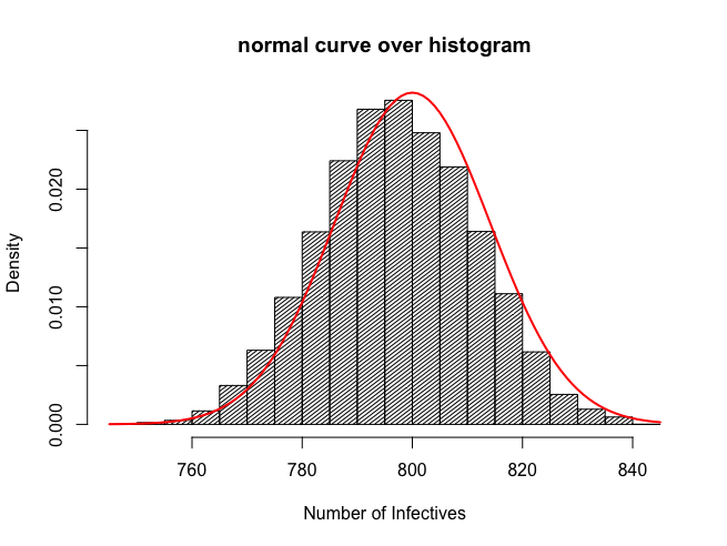
(a) $(n,m,R_{0})=(1000,2,5)$

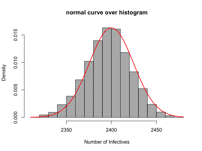
(b) $(n,m,R_{0})=(3000,2,5)$

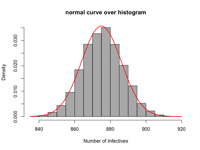
(c) $(n,m,R_{0})=(1000,2,8)$

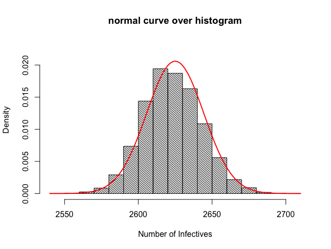
(d) $(n,m,R_{0})=(3000,2,8)$

Figure 2: Empirical distribution of SIS endemic level with CLT approximation

Figure 2 illustrates the distribution of $\{n^{-1}Y_{n}(t)|Y_{n}(t)>0,Y_{n}(t)\sim\mathbb{\tilde{q}}\}$.

4.1 Expected Mean Time to Extinction by CLT

Suppose that $R_{0}>1$ and $\{Y_{n}(t):t\geq 0\}$ is in quasi– equilibrium (meaning that $Y_{n}(t)$ enters endemic level). Then, the process will definitely mimic the deterministic model and with equilibrium point $\hat{y}=1-R_{0}^{-1}$.

Now, recall a drift function $F(y)$, where we define $y\in\mathbb{Z}$ in such a way that $\beta_{l}:\mathbb{Z}\rightarrow\left[0,\infty\right),l\in\Delta\subseteq\mathbb{Z},\sum_{l}\beta_{l}\left(y\right)<\infty$. In SIS, $\Delta=\{1,-1\}$ represents the possible transitions of the process, i.e., $1$ for infection to occur and $-1$ for removal to occur. Therefore,

$$F(y) =\beta_{1}(y)+(-1)\cdot\beta_{-1}(y)$$

$$=\lambda y(t)\cdot(1-y(t))-\gamma y(t)$$ (16)

Furthermore,

$$\partial F(y)=\left[\frac{\partial F(y)}{\partial y}\right] =\lambda(1-2y(t))-\gamma$$ (17)

and

$$G(y) =\beta_{1}(y)+\beta_{-1}(y)$$

$$=\lambda y(t)\cdot(1-y(t))+\gamma y(t).$$ (18)

Thus since we assume that the process is in quasi–equilibrium, $y(t)=\hat{y}$ for all $t\in\{t\geq 0:Y_{n}(t)\mid Y_{n}(0)\neq 0\sim\tilde{\boldsymbol{q}}\}$. Therefore,

$$\partial F(\hat{y}) =-(\lambda-\gamma),$$ (19)

$$G(\hat{y}) =2\cdot\frac{\gamma}{\lambda}(\lambda-\gamma).$$ (20)

Since (19) is continuous, then according to Theorem 4.1, for any $t\geq 0$,

$$\sqrt{n}\left(\frac{Y_{n}(t)}{n}-(1-R_{0}^{-1})\right)\xrightarrow{\text{\quad D \quad}}N(0,\sigma^{2}(t))$$ (21)

as $n\rightarrow\infty$ and $\sigma^{2}(t)$ must satisfy

$$\frac{d\sigma^{2}(t)}{dt} =2\cdot\frac{\gamma}{\lambda}(\lambda-\gamma)-2\cdot(\lambda-\gamma)\sigma^{2}(t)$$ (22)

with initial value $\sigma^{2}(0)=0$. Therefore, the solution of equation (22), for $t\rightarrow\infty$, is

$$\sigma^{2}(t)=\frac{\gamma}{\lambda}\left(1-e^{-2(\lambda-\gamma)t}\right)\rightarrow\frac{\gamma}{\lambda}=R_{0}^{-1}.$$ (23)

The eq.(21) is equivalent to

$$\sqrt{n}\left(\frac{Y_{n}(t)}{n}-(1-R_{0}^{-1})\right) \approx N(0,R_{0}^{-1})$$

$$\frac{Y_{n}(t)}{n}-(1-R_{0}^{-1}) \approx N\left(0,\frac{1}{nR_{0}}\right)$$

$$Y_{n}(t) \approx N\left((1-R_{0}^{-1})n,\frac{n}{R_{0}}\right)$$ (24)

for large $n$ and large $t$.

Suppose that $\mu_{n}=(1-R_{0}^{-1})n$ and $\sigma^{2}_{n}=\frac{\displaystyle n}{\displaystyle R_{0}}$ for simpler notations. Let $f_{n}$ and $F_{n}$ denote the pdf and cdf of $N(\mu_{n},\sigma_{n}^{2})$. Then using a continuity correction, we can approximate quasi-stationary distribution in (10) as follows

$$\tilde{q}_{1} \approx\frac{f_{n}(1)}{F_{n}\left(n+\displaystyle\frac{1}{2}\right)-F_{n}\left(\displaystyle\frac{1}{2}\right)}$$

$$=\displaystyle\frac{\displaystyle\frac{1}{\sqrt{2\pi\sigma_{n}^{2}}}e^{-\frac{(x-\mu_{n})^{2}}{2\sigma_{n}^{2}}}}{\displaystyle\int_{-\infty}^{n+\frac{1}{2}}\displaystyle\frac{1}{\sqrt{2\pi\sigma_{n}^{2}}}e^{-\frac{(x-\mu_{n})^{2}}{2\sigma_{n}^{2}}}dx-\displaystyle\int_{-\infty}^{\frac{1}{2}}\displaystyle\frac{1}{\sqrt{2\pi\sigma_{n}^{2}}}e^{-\frac{(x-\mu_{n})^{2}}{2\sigma_{n}^{2}}}dx}$$

$$=\frac{\frac{1}{\sigma_{n}}\phi\left(\frac{1-\mu_{n}}{\sigma_{n}}\right)}{\Phi\left(\frac{n+\frac{1}{2}-\mu_{n}}{\sigma_{n}}\right)-\Phi\left(\frac{\frac{1}{2}-\mu_{n}}{\sigma_{n}}\right)}$$ (25)

where $\phi(x)$ and $\Phi(x)$ are pdf and cdf of standardised normal distribution. Therefore, the approximate mean time to extinction of the SIS epidemic model by applying Theorem 4.1 is

$$E(T_{Q}) =\frac{1}{\gamma\tilde{q}_{1}}$$

$$\approx\left[\frac{\displaystyle\frac{\gamma}{\sigma_{n}}\phi\left(\frac{1-\mu_{n}}{\sigma_{n}}\right)}{\Phi\left(\displaystyle\frac{n+\frac{1}{2}-\mu_{n}}{\sigma_{n}}\right)-\Phi\left(\displaystyle\frac{\frac{1}{2}-\mu_{n}}{\sigma_{n}}\right)}\right]^{-1}$$ (26)

for large $n$ and large $t$.

5 Conclusion

We have successfully determined the approximation of expected mean time to extinction of SIS model using quasi–stationary distribution . An interesting result is that the empirical distribution of the SIS in endemic–stage followed normal distribution as the population size went to infinity. By using the CLT of Ethier and Kurtz, it turned out that the mean parameters of the SIS is the equilibrium points derived from solving deterministic’s ODE. This result was not surprising since we have showed in previous work that the stochastic models moved randomly around the deterministic model’s equilibrium point. Furthermore, the variances of the models converged to some positive constants since intuitively, as the population size went sufficiently large, the stochastic paths moved randomly around its endemic–equilibrium point.

6 Appendix A

First, we need to show that for $i,j\in T$, $\boldsymbol{E}_{i}\boldsymbol{E}_{j}=\begin{cases}\boldsymbol{E}_{i}&\text{if }i\neq j\\ \boldsymbol{0}&\text{if }i\neq j\end{cases}.$

Proof.

Note that since $\boldsymbol{u}_{i}$ is orthonormal, then

$$\boldsymbol{E}_{i}\boldsymbol{E}_{j} =\boldsymbol{W}^{-1/2}\left(\boldsymbol{u}_{i}\boldsymbol{u}_{i}^{T}\right)\boldsymbol{W}^{1/2}\boldsymbol{W}^{-1/2}\left(\boldsymbol{u}_{j}\boldsymbol{u}_{j}^{T}\right)\boldsymbol{W}^{1/2}$$

$$=\left(\boldsymbol{W}^{-1/2}\boldsymbol{u}_{i}\right)\left(\boldsymbol{u}_{i}^{T}\boldsymbol{u}_{j}\right)\left(\boldsymbol{u}_{j}^{T}\boldsymbol{W}^{1/2}\right)$$

$$=\begin{cases}\boldsymbol{E}_{i}&\quad\text{if }i=j\\ \boldsymbol{0}&\quad\text{if }i\neq j\end{cases}$$ (27)

since $\boldsymbol{u}_{i}^{T}\boldsymbol{u}_{j}=\begin{cases}1&\quad\text{if }i=j\\ 0&\quad\text{if }i\neq j\end{cases}.$ ∎

And secondly, we need to show that $\displaystyle\sum_{i=1}^{n}\boldsymbol{E}_{i}=I_{n\times n}$.

Proof.

Note that,

$$\sum_{i=1}^{n}\boldsymbol{E}_{i} =\left(\boldsymbol{W}^{-1/2}\boldsymbol{u}_{1}\right)\left(\boldsymbol{u}_{1}^{T}\boldsymbol{W}^{1/2}\right)+\ldots+\left(\boldsymbol{W}^{-1/2}\boldsymbol{u}_{n}\right)\left(\boldsymbol{u}_{n}^{T}\boldsymbol{W}^{1/2}\right)$$

$$=\boldsymbol{W}^{-1/2}\left(\boldsymbol{u}_{1}\boldsymbol{u}_{1}^{T}+\ldots+\boldsymbol{u}_{n}\boldsymbol{u}_{n}^{T}\right)\boldsymbol{W}^{1/2}$$

$$=\boldsymbol{W}^{-1/2}I_{n\times n}\boldsymbol{W}^{1/2}=I_{n\times n}.$$ (28)

∎

Note that $\exp{(\boldsymbol{Q}t)}=\displaystyle\sum_{k=0}^{\infty}\frac{\displaystyle\boldsymbol{Q}^{k}t^{k}}{\displaystyle k!}$. Then, for any $i\in T$,

$$\exp{(\lambda_{i}t\boldsymbol{E}_{i})} =\sum_{k=0}^{\infty}\frac{(\lambda_{i}t)^{k}\boldsymbol{E}_{i}^{k}}{k!}=\boldsymbol{E}_{i}\sum_{k=0}^{\infty}\frac{(\lambda_{i}t)^{k}}{k!}=\exp{(\lambda_{i}t)}\boldsymbol{E}_{i}.$$

7 Appendix B

Notice $\boldsymbol{E}_{i}=\left(\boldsymbol{W}^{-1/2}\boldsymbol{u}_{i}\right)\left(\boldsymbol{u}_{i}^{T}\boldsymbol{W}^{1/2}\right)$. Then,

$$\boldsymbol{Q}_{TT} =\sum_{i=1}^{n}\lambda_{i}\left(\boldsymbol{W}^{-1/2}\boldsymbol{u}_{i}\right)\left(\boldsymbol{u}_{i}^{T}\boldsymbol{W}^{1/2}\right)$$

$$\left(\boldsymbol{u}_{i}^{T}\boldsymbol{W}^{1/2}\right)\boldsymbol{Q}_{TT} =\sum_{i=1}^{n}\lambda_{i}\underbrace{\left(\boldsymbol{u}_{i}^{T}\boldsymbol{W}^{1/2}\right)\left(\boldsymbol{W}^{-1/2}\boldsymbol{u}_{i}\right)}_{=1}\left(\boldsymbol{u}_{i}^{T}\boldsymbol{W}^{1/2}\right)$$

$$=\sum_{i=1}^{n}\lambda_{i}\left(\boldsymbol{u}_{i}^{T}\boldsymbol{W}^{1/2}\right).$$

Hence, $\left(\boldsymbol{u}_{i}^{T}\boldsymbol{W}^{1/2}\right)$ is the left-eigenvector of $\boldsymbol{Q}_{TT}$.

8 References

References

• [1] H. Andersson and T. Djehiche, “Stochastic Epidemics in Dynamic Populations: Quasi-Stationary and Extinction”, J. Math. Bio.  41, 559–580 (2000).
• [2] H. Andersson and B. Djehiche, “A Threshold Limit Theorem for the Stochastic Logistic Epidemic”, J. Appl. Prob.  35, 662–670 (1998).
• [3] N. T. Bailey, The Mathematical Theory of Infectious Diseases and its Applications, 2nd edition (Griffin, London, 1975).
• [4] F. G. Ball, “The Threshold Behaviour of Epidemic Models”, J. Appl. Prob.  20, 227–241 (1983).
• [5] F. G. Ball, Epidemic Thresholds. Encyclopedia of Biostatistics. 3. (John Wiley & Sons, Chichester, 1998).
• [6] F. G. Ball, T. Britton, and P. Neal, “On Expected Durations of Birth-Death Processes, with Application to Branching Processes and SIS Epidemics”, Submitted J. Appl. Prob. 53, 203–215 (2016).
• [7] F. G. Ball and O. D. Lyne, “Optimal Vaccination Policies for Stochastic Epidemics among a Population of Households”, Submitted Math. Bioscie.  177–178, 333–354 (2002).
• [8] P. G. Ballard, N. G. Bean, J. V. Ross, “The Probability of Epidemic Fade-Out is Non-Monotonic in Transmission Rate for Markovian SIR Model with Demography”, Submitted J. Theoretical Bio.  393, 170–178 (2016).
• [9] H. Andersson and T. Britton, Stochastic Epidemic Models and Their Statistical Analysis (Springer, New York, 2000).
• [10] T. Britton and P. Neal “The Time to Extinction for an SIS-houshold-epidemic Model”, Submitted J. Math. Bio.  61, 763–779 (2010).
• [11] D. Clancy and P. K. Pollett, “A Note on Quasi-Stationary Distributions of Birth-Death Processes and the SIS Logistic Epidemic”, Submitted J. Appl. Prob.  40, 821–825 (2003).
• [12] J.N. Darroch and E. Seneta, “On Quasy-Stationary Distributions in Absorbing Discrete-Time Finite Markov Chains”, Submitted J. Appl. Prob.  2, 88–100 (1965).
• [13] J.N. Darroch and E. Seneta, “On Quasy-Stationary Distributions in Absorbing Continuous-Time Finite Markov Chains”, Submitted J. Appl. Prob.  4, 192–196 (1967).
• [14] S. N. Ethier and T. G. Kurtz, Markov Processes Characterization and Convergence (Wiley, New York, 1982).
• [15] s.‘Karlin, A First Course in Stochastic Processes. 2nd ed. (Academic Press Inc., California, 1975).
• [16] F. P. Kelly, Reversibility and Stochastic Networks (Cambridge University Press, Cambridge, 2011).
• [17] D. G. Kendall, “On the Generalized Birth and Death Process”, The Annals of Mathematical Statistics  19, 1–15 (1948).
• [18] R. J. Kryscio and C. Lefévre, “On the Extinction of SIS Stochastic Logistic Epidemic”, J. Appl. Prob.  26, 685–694 (1989).
• [19] I. Nåsell, “Stochastic Models of Some Endemic Infections”, Math. Bioscie. 179, 1–19 (2002).
• [20] R.H. Norden, “On the Distribution of The Time to Extinction in the Stochastic Logistic Population Model”, Adv. in Appl. Prob.  14, 687–708 (1982).
• [21] S.M. Ross, Introduction to Probability Models. 9th ed. (Elsevier Inc., London, 2007).
• [22] K. Susvitasari, “Comparing the Behaviour of Deterministic and Stochastic Model of SIS Epidemic”, arXiv:1803.01497 [q-bio.PE]