boxed logical pages=1, 1 border code= ,border shrink=,resized width=.95,resized height=.95,center=

Modeling and analysis of nonfunctional requirements is crucial in automotive systems. East-adl is an architectural language dedicated to safety-critical automotive system design. We have previously modified East-adl to include energy constraints and transformed energy-aware timed (ET) behaviors modeled in Simulink/ Stateflow into Uppaal models amenable to formal verification. Previous work is extended in this paper by including support for Simulink Design Verifier (SDV), i.e., the ET constraints are translated into proof objective models that can be verified using SDV. Furthermore, probabilistic extension of East-adl constraints is defined and the semantics of the extended constraints is translated into verifiable Uppaal models with stochastic semantics for formal verification. A set of mapping rules are proposed to facilitate the guarantee of translation. Verification & Validation are performed on the extended timing and energy constraints using SDV and Uppaal-smc. Our approach is demonstrated on a cooperative automotive system case study.

Keywords: East-adl, Uppaal-smc, Simulink Design Verifier

Contents

1. 1 Introduction
2. 2 Preliminary
3. 3 Case Study
4. 4 Modeling Non-functional Behaviors in Simulink & Stateflow
   1. 4.1 Behavioral Modeling of $f_{p}$s in Simulink & Stateflow
   2. 4.2 Modeling Timing and Energy Constraints in Simulink/Stateflow
5. 5 Timing & Energy Requirements Translation in SDV
   1. 5.1 LTL Properties
   2. 5.2 Timing Constraints in SDV
   3. 5.3 Energy Constraints in SDV
6. 6 Modeling Functional Behaviours in Uppaal-smc
7. 7 (Non)-functional Property Translation in Uppaal-smc
   1. 7.1 Probabilistic Timing Constraints Translation
   2. 7.2 Energy Constraint Estimation
8. 8 Experiment and Verification
9. 9 Verification of Comparison Constraint in Uppaal-smc
10. 10 Related Work
11. 11 Conclusion
12. Acknowledgment

List of Figures

1. 2.1 General verification models in SDV
2. 2.2 Simulink Blocks used for property modeling
3. 3.1 Cooperative Automotive System
4. 3.2 East-adl Architecture of CAS
5. 4.1 Top-level diagram of CAS Simulink & Stateflow model
6. 4.2 Stateflow chart of v1Controller
7. 4.3 leader state in v1Controller
8. 4.4 follower state in v1Controller
9. 4.5 userCtrl state in v1Controller
10. 4.6 Simulink & Stateflow model of localEnv
11. 4.7 Simulink & Stateflow model of DriverBehavior
12. 4.8 Simulink & Stateflow model of VehicleDynamic
13. 4.9 Simulink & Stateflow model of ComDevice
14. 4.10 Timing constraints modeling
15. 4.11 Cumulative and Noncumulative constraint
16. 4.12 Periodic constraint modeling
17. 5.1 Bounded Always and Eventually property
18. 5.2 p Until q: G (F${}_{[0,\ t]}$ q $\wedge$ ($\neg$q $\implies$ p))
19. 5.3 Functional Property: When auto is true and msg is false for 200ms, userCtrl should become true within 200ms.
20. 5.4 Property: If the dis12 is smaller than safeDis, v2dec should be true within 500ms.
21. 5.5 Synchronization timing constraint
22. 5.6 Timing constraints translation
23. 5.7 Sporadic timing constraint
24. 5.8 R30: if the message transmission is failed (msgNormal == false) when the vehicle runs in auto-mode, for the next 20 seconds, the vehicle should not run automatically, i.e., auto == false
25. 5.9 Cumulative Periodic Timing Constraint
26. 5.10 Non-cumulative Periodic Timing Constraint
27. 5.11 Energy constraint
28. 6.1 STA of SignRecognition
29. 6.2 STA of VehicleDynamic
30. 6.3 STA for modeling ComDevice
31. 6.4 STA for modeling DriverBehaviour
32. 6.5 STA of Controller
33. 6.6 STA of Control state
34. 6.7 STA for deciding whether the message is missing
35. 6.8 STA for modeling Communication state
36. 6.9 STA for modeling leader state
37. 6.10 STA for modeling substates of leader state
38. 6.11 STA for modeling substates of leader state
39. 6.12 STA of turnLeft state
40. 6.13 STA of turnRight state
41. 6.14 STA of follower state
42. 6.15 STA of follower state
43. 6.16 STA for modeling substates of straight state
44. 6.17 STA for modeling substates of turn state
45. 6.18 STA for modeling userctrl state
46. 6.19 STA of UserCtrl state
47. 6.20 STA for modeling substates of straight state
48. 6.21 STA for modeling substates of turnleft state
49. 6.22 STA for modeling substates of turnright state
50. 7.1 Probabilistic Extension of Timing Constraints in Uppaal-smc
51. 7.2 Energy estimation of v1Controller
52. 7.3 Energy constraints on sensors in Uppaal-smc
53. 8.1 When v1 runs automatically and if there is no message received by the vehicle for a certain time, the running mode of the vehicle should be changed to manual mode within a certain time: G (G_[0,200] v1.Auto==true $\wedge$ v1.msg == false $\implies$ F_[0,2000] v1.userCtrl == true)
54. 8.2 When v1 runs automatically with a constant speed, if it detects a stop sign, it should start to brake in 500ms: G (v1.Auto == true $\wedge$ v1.const == true $\wedge$ signType == 5 $\implies$ F_[0,500] v1.stop == true)
55. 8.3 When the lead vehicle (v1) runs automatically with a constant speed, if it detects left turn sign, it should start to turn left in 200ms: G (v1.auto == true $\wedge$ v1.const == true $\wedge$ signType == 4 $\implies$ F_[0,200] v1.turnLeft == true)
56. 8.4 If v1 is driven by the driver and it is running with a constant speed, the driver steers to the left, the vehicle will turn left within 200ms: G (v1.userCtrl == true $\wedge$ v1.const == true $\wedge$ v1.steerReq == 1 $\implies$ F_[0,200] v1.turnLeft == true)
57. 8.5 If v1 is driven by the driver and it is running at a constant speed, the driver brakes the car, the vehicle will slow down. G: (v1.userCtrl == true $\wedge$ v1.const == true $\wedge$ v1.brakeReq == 2 $\implies$ F_[0,200] v1.brake == true)
58. 8.6 When v1 is driven by the driver and it is running at a constant speed, if the driver gears up, the vehicle will accelerate. G (v1.userCtrl == true $\wedge$ v1.const == true $\wedge$ v1.gearReq $>$ v1.gear $\implies$ F_[0,200] v1.acc == true)
59. 8.7 When the vehicles are running horizontally, following vehicle should not run ahead of lead vehicle. G (v1.dx == 1 $\wedge$ v2.dx == 1 $\wedge$ v3.dx == 1 $\implies$ v1.x $>$ v2.x)
60. 8.8 When the lead vehicle detects a stop sign, the three vehicles should stop in 5s. G (v1.auto == true $\wedge$ signType == 5 $\implies$ F_[0,5000] v1.static == true $\wedge$ v2.static == true $\wedge$ v3.static==true)
61. 8.9 Noncumulative Periodic timing constraint: A Periodic acquisition of VehicleDynamic of v1 must be carried out for every 50 ms with a jitter 10 ms. G (v1.velIn == true $\implies$ v1.velIn == false U_{[40, 60]} v1.velIn == true)
62. 8.10 Cumulative Periodic timing constraint of R27
63. 8.11 Sporadic constraint: After the running mode of the lead vehicle is changed to manual mode because of the failed message transmission, the driver should not change it into auto mode within 20 seconds. G (v1.msgNormal == false $\implies$ v1.auto == false U${}_{[2000,\ \infty]}$) v1.auto == true
64. 8.12 An Execution constraint applied on v3Controller, which measured from the inputs ports Avel to output ports gearReq, torqueReq, and brake, should be between 100 ms and 300 ms; G (v3.ctrlIn $\implies$ F_[100,300] v3.ctrlOut)
65. 8.13 An Execution constraint applied on v3Controller, which measured from the inputs ports Avel to output ports gearReq, torqueReq, and brake, should be between 100 ms and 300 ms; G (v3.ctrlIn $\implies$ F_[100,300] v3.ctrlOut)
66. 8.14 An Execution constraint applied on ComDevice of v1, which measured from the inputs ports torqueSet, gearSet and brake to output ports wheelSpeed, direct should be between 100 ms and 150 ms; G (v1.sdrIn $\implies$ F_[100,300] v1.sdrOut
67. 8.15 Observer STA of R1 and its triggering
68. 8.16 Uppaal-smc STAs for timing constraints verification
69. 8.17 Uppaal-smc STAs for End-to-End timing constraints verification
70. 8.18 Uppaal-smc STAs for End-to-End timing constraints verification
71. 8.19 CE in SDV: In (b), leadVe.y equals to followVe.y) from 0 to 8s, which indicates that the two vehicles run in the same lane. In (a), signType becomes “turn left (4)” at 8s and the lead vehicle begins to turn left. However, the following vehicle turns left at a different location (leadVe.x is not equal to followVe.x at 9s). Hence, the “x” is unequal after turning, which means that the two vehicles run on different lanes. Thus R23 and R24 is violated.
72. 8.20 CE in SMC: At the beginning, three vehicles run towards direction (1,0). The three values of posy are the same, which indicates that the three vehicles are in the same lane. After a left turn sign is detected, the lead vehicle starts to turn left. Since the first follower turns left at (184, 0) and the second turns left at (157, 0), the three values of posx are not equal after turning, which indicates the three vehicle are not running in the same lane. Thus R5 is violated.
73. 8.21 Probabilistic distribution of the expected energy consumption
74. 8.22 Total energy consumption estimation of the lead vehicle

Chapter 1 Introduction

Model-driven development is rigorously applied in automotive systems in which the software controllers interact with physical environments. The continuous time behaviors (evolved with various energy rates) of those systems often rely on complex dynamics as well as on stochastic behaviors. Formal verification and validation (V&V) technologies are indispensable and highly recommended for development of safe and reliable automotive systems [1, 2]. Conventional V&V, i.e., testing and model checking have limitations in terms of assessing the reliability of hybrid systems due to both the stochastic and non-linear dynamical features. To ensure the reliability of safety critical hybrid dynamic systems, statistical model checking (SMC) techniques have been proposed [3, 4, 5]. These techniques for fully stochastic models validate probabilistic performance properties of given deterministic (or stochastic) controllers in given stochastic environments.

East-adl [6, 7] is a domain specific language that provides support for architectural modeling of automotive embedded systems. A system in East-adl is described by Functional Architectures (FA) at different abstraction levels. The FA are composed of a number of interconnected functionprototypes ($f_{p}$s), and the $f_{p}$s have ports and connectors for communication. East-adl relies on external tools for the analysis of specifications related to requirements. For example, behavioral description in East-adl is captured in external tools, i.e., Simulink/Stateflow[8]. The latest release of East-adl has adopted the time model proposed in the Timing Augmented Description Language (Tadl2) [9]. Tadl2 allows for the expression and composition of timing constraints, e.g., periodic, end-to-end delay, and synchronization constraints on top of East-adl models.

In this paper, we propose a model-driven approach to support formal analysis of energy and timed (ET) requirements for automotive systems at the design level: 1. The ET constraints in East-adl are interpreted in Simulink/Stateflow (S/S) and provide corresponding modeling extensions in S/S; 2. The ET requirements, specified in temporal logics, are translated into proof objective models to perform formal verification using SDV; 3. Probabilistic extension of East-adl/Tadl constraints is defined and the semantics of the extended constraints (Xtc) is translated into verifiable Uppaal-smc [10] models with stochastic semantics for formal verification; 4. A set of mapping rules are proposed to facilitate the guarantee of translation; 5. Simulation and V&V are performed on the Xtc and energy constraints using SDV and Uppaal-smc. Our approach is demonstrated on the cooperative automotive system (CAS) case study.

The paper is organized as follows: Chap. 2 presents an overview of Simulink, SDV, and Uppaal-smc. The CAS is introduced as a running example in Chap. 3. Chap. 4, 5, 6 and 7 describe a set of translation patterns and how our approaches provide support for formal analysis at the design level. The applicability of our method is demonstrated by performing verification on the CAS case study in Chap. 8. Chap. 10 and Chap. 11 present related work and conclusion.

Chapter 2 Preliminary

In our framework, Simulink and Embedded Matlab (EML) are utilized for modeling purposes. Verification and experiment are performed by SDV and Uppaal-smc.

Simulink and SDV: Simulink [8] is a synchronous data flow language, which provides different types of blocks, i.e., primitive-, control flow-, and temporal-blocks with predefined libraries for modeling and simulation of dynamic systems and code generation. Simulink supports the definition of custom blocks via Stateflow diagrams or user-defined function blocks written in EML, C, and C++. SDV is a plug-in to Prover, which is a formal verification tool that performs reachability analysis on Simulink/Stateflow model. The satisfiability of each reachable state is determined by a SAT solver. A proof objective model is specified in Simulink/SDV and illustrated in Fig.2.1. A set of data (predicates) on the input flows of System is constrained via $\ll$Proof Assumption$\gg$ blocks during proof construction. A set of proof obligations is constructed via a function $F$ block and the output of $F$ is specified as input to a property $P$ block. $P$ passes its output signal to an $\ll$Proof Objective$\gg$ block and returns true when the predicates set on the input data flows of the outline model are satisfied. Whenever $\ll$Proof Objective$\gg$ (P block) is utilized, SDV verifies whether the specified input data flow is always true. The underlying Prover engine allows the formal verification of properties for a given model. Any failed proof attempt ends in the generation of a counterexample representing an execution path to an invalid state. A harness model is generated to analyze the counterexample and refine the model.

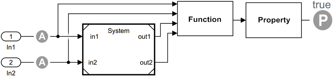
Figure 2.1: General verification models in SDV

Fig.2.2 shows blocks in SDV that can be employed in properties specification. $\ll$Implies$\gg$ block (Fig.2.2.(a)) allows to specify a condition to produce a certain response: if A is true and B is false, the output is false; for all other pairs of A and B, the outputs are true. $\ll$Within Implies$\gg$ block (Fig.2.2.(b)) verifies the property that the response occurs within a given duration. This block captures the within implication by observing whether the Obs input is true for at least one step within each true duration of In. If Obs is always false within a particular input true duration of In, the output becomes false for one time step following the input true duration. As shown in Fig.2.2.(c), the two blocks always appear in pairs with the same tags. The output signal from Block A goes to the $\ll$Goto$\gg$ block tagged with A. $\ll$Goto$\gg$ block then passes that signal to the $\ll$From$\gg$ block tagged with A. Block B receives the signal from the $\ll$From$\gg$ block.

(a) Implies

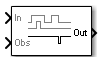
(b) Within Implies

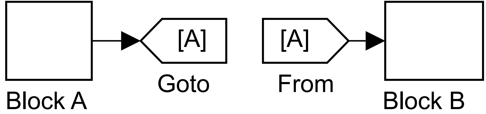
(c) From and Goto

Figure 2.2: Simulink Blocks used for property modeling

Uppaal-smc provides probabilistic analysis of properties based on statistical estimation of system models. By monitoring simulations of an hybrid system and using the statistic result to determine whether the properties are satisfied on top of the system model, an exhaustive exploration of the state-space of the system can be avoided. Uppaal-smc represents systems via networks of Timed Automata (TA) whose behaviours depend on both stochastic and non-linear dynamical features. Its clocks evolve with various rates, such rates can be specified with ordinary differential equations. Uppaal-smc provides a number of queries related to the stochastic interpretation of TA (STA) [5]. The following four queries are sufficient to perform V&V on timing and energy constraints in East-adl, where $N$ and $bound$ indicate the number of simulations and the simulation time for each simulation respectively.

1. Probability Estimation estimates the probability that a requirement property $\phi$ is satisfied for a given STA model within the time bound: $Pr[bound]$ $\phi$;

2. Hypothesis Testing checks if the probability of $\phi$ is satisfied over a given probability $P_{0}$: $Pr[bound]$ $\phi$ $\geq$ $P_{0}$;

3. Simulations: Uppaal-smc runs multiple simulations on the system model and the $k$ (state-based) properties/expressions $\phi_{1},...,\phi_{k}$ are monitored and visualized along the simulations: $simulate$ $N$ $[\leq$ $bound]\{\phi_{1},...,\phi_{k}\}$;

4. Expected Value evaluates the minimal or maximal value of a clock or an integer value while Uppaal-smc checks the STA model: $E[bound;N](min:\phi)$ or $E[bound;N](max:\phi)$.

Chapter 3 Case Study

A Cooperative Automotive System (CAS) is adopted as our running example where sensing and actuation are distributed over a number of vehicles, which is illustrated in Fig.3.1. A vehicle can be either a lead vehicle (leadVe) or a following vehicle (followVe) depends on its absolute position. We name the first vehicle as v1, the vehicle in the middle as v2 and the last vehicle v3. Communication between vehicles are realized by the Dedicated Short-Range Communication (DSRC), which is a wireless communication technology specifically dedicated for message transmission among automotive systems. The lead vehicle can either run automatically (auto mode) by detecting traffic signs on the road or be driven by the driver (userCtrl mode). Any two adjacent vehicles should be distant enough to avoid rear-end collision and close enough to guarantee the communication quality.

The requested vehicle motion is based on driver’s input, detected environment (e.g., traffic sign) and running situation. The vehicle movement can be either horizontal or vertical and the position of each vehicle is represented by two-dimension coordinates (x, y) in Cartesian coordinate system, where x and y are distances measured from vehicle to two fixed perpendicular directed lines respectively. Ideally, the following vehicle should maintain the same movement as the vehicle ahead and behaves similarly, e.g., when a lead vehicle accelerates, the following vehicles should be able to accelerate to a similar extent.

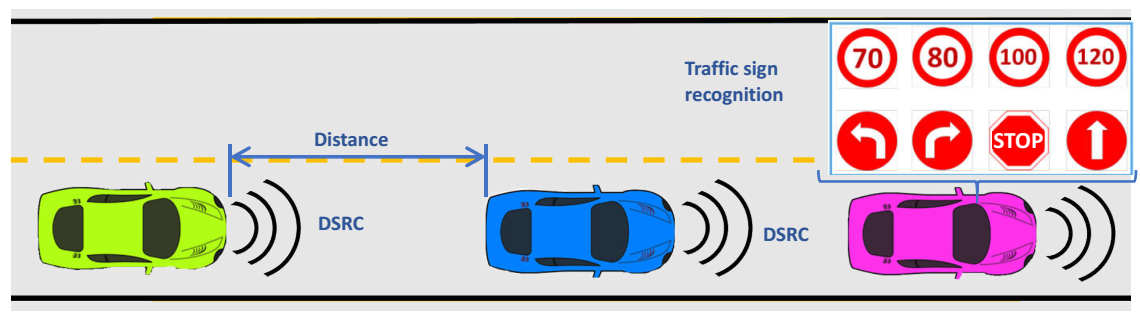
Figure 3.1: Cooperative Automotive System

Fig.3.2(a) shows the East-adl model of the CAS, which consists of cooperative environment (CoopEnv) and local environments, left and middle, and the software controllers of three vehicles, right. The three LocalEnv $f_{p}$s receive information of positions and the traffic sign from the CoopEnv. Each lead vehicle sends its own position and velocity to its adjacent following vehicle. The functionality of an individual vehicle, augmented with timing/energy constraints and viewed as FunctionDesignArchitecture (FDA) in 3.2(b), consists of the following $f_{p}$s (components): ComDevice represents the DSRC device for vehicle to send and receive messages. SignRecDevice analyzes the detected images and computes desired images (sign types). VeModeDevice reads the driver’s requests by means of pedals (brakeReq), steering wheel (steerReq), gear (gearReq) and a switch (driverState) which indicates whether the driver intends to drive. v1Controller determines how the torque and gear of the vehicle are adjusted based on the received information. VeDynamicDevice specifies the kinematics behaviors of the vehicle based on engine torque, brake, steer and gear. The value of signType ranges from 0 to 5, which represents “straight”, “min/max speed limit”, “left/right turn ahead” and “stop” signs respectively.

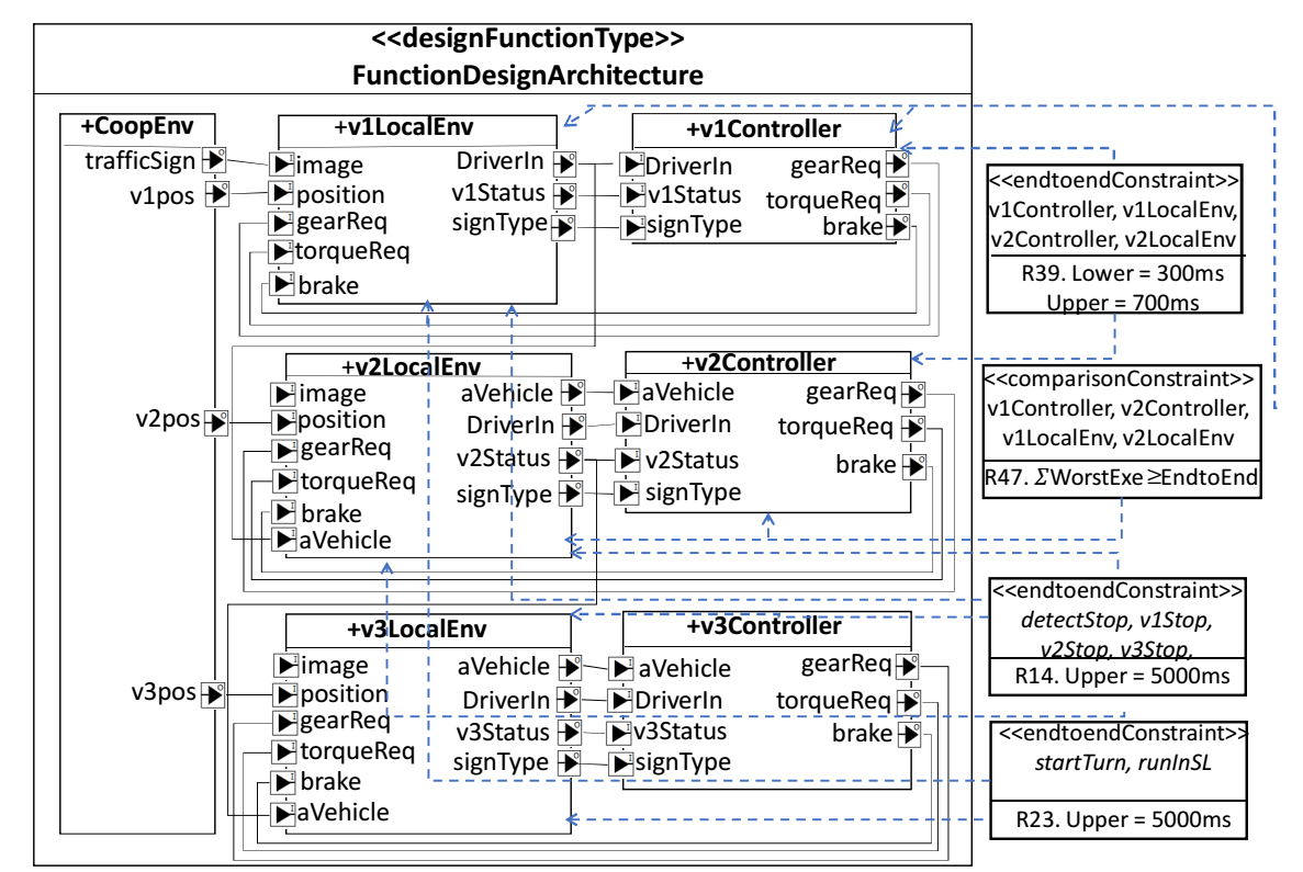
(a) Architecture of cooperative automotive system model

(b) Function architecture of a vehicle

Figure 3.2: East-adl Architecture of CAS

We consider the following functional and non-functional properties, which includes Execution, End-to-End, Synchronization, Periodic, Sporadic and
Comparison timing and Energy constraints, on top of the CAS EAST-ADL model, which are sufficient to capture the constraints described in Fig.3.2. Energy constraint refers to the battery consumption of an individual vehicle in CAS.

• R1. When v1 runs automatically and if there is no message received by the vehicle for a certain time, the running mode of the vehicle should be changed to manual mode within a certain time.

• R2. When v2 runs automatically and if there is no message received by the vehicle for a certain time, the running mode of the vehicle should be changed to manual mode within a certain time.

• R3. When v3 runs automatically and if there is no message received by the vehicle for a certain time, the running mode of the vehicle should be changed to manual mode within a certain time.

• R4. When v1 runs automatically at a constant speed, if it detects a stop sign, it should start to brake in 500ms.

• R5. When v1 runs automatically at a constant speed, if it detects left turn sign, it should start to turn left in 200ms.

• R6. When v1 runs automatically at a constant speed, if it detects right turn sign, it should start to turn right in 200ms.

• R7. If v1 is driven by the driver and it is running with a constant speed, the driver steers to the left, the vehicle will turn left within 200ms.

• R8. If v1 is driven by the driver and it is running at a constant speed, the driver steers to the right, the vehicle will turn right within 200ms.

• R9. If v1 is driven by the driver and it is running at a constant speed, the driver brake the car, the vehicle will slow down.

• R10. When v1 is driven by the driver and it is running at a constant speed, if the driver gears up, the vehicle will accelerate.

• R11. When v1 is driven by the driver and it is running at a constant speed, if the driver gears down, the vehicle will decelerate.

• R12. v2 should not run ahead of v1.

• R13. v3 should not run ahead of v2.

• R14. When the lead vehicle detects a stop sign, the three vehicles should stop in 5s.

• R15. When the vehicles are running straight with a constant speed, if v2 runs slower than v1, it should start to accelerate within a certain time.

• R16. When the vehicles are running straight with a constant speed, if v3 runs slower than v2, it should start to accelerate within a certain time.

• R17. When the vehicles are running straight with a constant speed, if v2 runs faster than v1, it should start to decelerate within a certain time.

• R18. When the vehicles are running straight with a constant speed, if v3 runs faster than v2, it should start to decelerate within a certain time.

• R19. If the distance between v1 and v2 is larger than 500m, v2 should accelerate within a certain time, e.g. 200ms.

• R20. If the distance between v2 and v3 is larger than 500m, v3 should accelerate within a certain time, e.g. 200ms.

• R21. If the distance between v1 and v2 is smaller than the safety distance, v2 should decelerate within a certain time, e.g. 500ms.

• R22. If the distance between v2 and v3 is smaller than the safety distance, v3 should decelerate within a certain time, e.g. 500ms.

• R23. When v1 starts to turn left, v1 and v2 should finish turning and run in the same lane within a given time.

• R24. When v2 starts to turn left, v2 and v3 should finish turning and run in the same lane within a given time.

• R25. When v1 starts to turn right, v1 and v2 should finish turning and run in the same lane within a given time.

• R26. When v2 starts to turn right, v2 and v3 should finish turning and run in the same lane within a given time.

• R27. A Periodic acquisition of VehicleDynamic of v1 must be carried out for every 50 ms with a jitter 10 ms.

• R28. A Periodic acquisition of VehicleDynamic of v2 must be carried out for every 50 ms with a jitter 10 ms.

• R29. A Periodic acquisition of VehicleDynamic of v3 must be carried out for every 50 ms with a jitter 10 ms.

• R30. Sporadic constraint: After the running mode of v1 is changed to manual mode because of the failed message transmission, the driver should not change it into auto mode within 20 seconds.

• R31. Sporadic constraint: After the running mode of v2 is changed to manual mode because of the failed message transmission, the driver should not change it into auto mode within 20 seconds.

• R32. Sporadic constraint: After the running mode of v3 is changed to manual mode because of the failed message transmission, the driver should not change it into auto mode within 20 seconds.

• R33. An Execution constraint applied on v1Controller, which measured from the input port Avel to output ports gearReq, torqueReq and brake, should be between 100 ms and 300 ms;

• R34. An Execution constraint applied on v2Controller, which measured from the input port Avel to output ports gearReq, torqueReq and brake, should be between 100 ms and 300 ms;

• R35. An Execution constraint applied on v3Controller, which measured from the input port Avel to output ports gearReq, torqueReq and brake, should be between 100 ms and 300 ms;

• R36. An Execution constraint applied on ComDevice of v1, which measured from the input ports Avel, Apos, Adirect and pos to output ports Avel, Apos, Adirect and pos should be between 50 ms and 100 ms;

• R37. An Execution constraint applied on ComDevice of v2, which measured from the input ports Avel, Apos, Adirect and pos to output ports Avel, Apos, Adirect and pos should be between 50 ms and 100 ms;

• R38. An Execution constraint applied on ComDevice of v3, which measured from the input ports Avel, Apos, Adirect and pos to output ports Avel, Apos, Adirect and pos should be between 50 ms and 100 ms;

• R39. An End-to-End is measured from v1Controller to v2Controller. The time interval is bounded with a minimum value of 300 ms and a maximum value of 700 ms;

• R40. An End-to-End is measured from v2Controller to v3Controller. The time interval is bounded with a minimum value of 300 ms and a maximum value of 700 ms;

• R41. An End-to-End constraint measured from input port position of v1LocalEnv to output ports gearReq, torqueReq and brake of v1Controller should be limited within [200, 500]ms;

• R42. An End-to-End constraint measured from input port position of v2LocalEnv to output ports gearReq, torqueReq and brake of v2Controller should be limited within [200, 500]ms;

• R43. An End-to-End constraint measured from input port position of v3LocalEnv to output ports gearReq, torqueReq and brake of v3Controller should be limited within [200, 500]ms;

• R44. Synchronization constraint: The position and velocity of the vehicle and its lead vehicle (pos, vel, Apos and Avel ports on v1Controller) must be detected by v1Controller within a given time window, i.e., the tolerated maximum constraint = 200 ms;

• R45. Synchronization constraint: The position and velocity of the vehicle and its lead vehicle (pos, vel, Apos and Avel ports on v2Controller) must be detected by v2Controller within a given time window, i.e., the tolerated maximum constraint = 200 ms;

• R46. Synchronization constraint: The position and velocity of the vehicle and its lead vehicle (pos, vel, Apos and Avel ports on v3Controller) must be detected by v3Controller within a given time window, i.e., the tolerated maximum constraint = 200 ms;

• R47. A Comparison constraint: The execution time interval measured from
  v1Controller to v2Controller needs to be larger than or equal to the sum of the worst-case execution times of the $f_{p}$s.

• R48. Energy constraint: The maximum battery energy consumption for the braking of a vehicle should be less than 30kJ;

• R49. Energy constraint: The maximum battery energy consumption for the controller to decide its movement for once should be less than 30J;

• R50. Energy constraint: The maximum battery energy consumption for ComDevice to get/send signals for once should be less than 5J;

According to the East-adl meta-model, the timing constraint describes a design constraint, but has the role of a property, requirement or validation result, based on its Context [6]. The Tadl meta-model is integrated with the East-adl meta-model and is supplemented with structural concepts from East-adl. The East-adl/Tadl constraints contain the identifiable state changes as Events. The causality related events are contained as a pair by EventChains. Based on Event and EventChains, data dependencies, control flows, and critical execution paths are represented as additional constraints for the East-adl functional architectural model, and apply timing constraints on these paths.

Sporadic constraint specifies a minimum delay min between any two consecutive occurrences of an event. Execution constraint restricts the time interval between inputs and outputs of a $f_{p}$, which can be specified using lower, upper values given as Execution constraint. End-to-End constraint gives duration bounds (minimum and maximum) between two events source and target. The time intervals between source event and target event should satisfy lower, upper values given as End-to-End constraint. Synchronization constraint describes how tightly the occurrences of a group of events follow each other. All events must occur within a sliding window, specified by the tolerance attribute, i.e., the maximum time interval allowed between events. Comparison constraint specifies the comparison relation (including $<$, $\leq$, $=$, $\geq$ and $>$) among timing expressions. Periodic constraint states that the period of successive occurrences of a single event must have a length of at least a lower and at most an upper time interval. The interval is given as Periodic constraint. There are two types of Periodic timing constraints: cumulative (Cumu_Periodic) and non-cumulative timing constraints (Noncumu_Periodic). Those (non)-functional properties are formally specified and verified in the following sections.

Chapter 4 Modeling Non-functional Behaviors in Simulink & Stateflow

4.1 Behavioral Modeling of $f_{p}$s in Simulink & Stateflow 

Based on the East-adl architectural model of CAS, the functional and non-functional behaviours of $f_{p}$s is constructed with Stateflow chart and Simulink blocks. The architecture of Simulink/Stateflow model can be seen in Fig.4.1. v1Controller $f_{p}$ is modeled as a Stateflow chart while localEnv, CoopEnv are modeled as Simulink subsystems with a number of mathematical and descriptive blocks provided in Simulink block library.

Figure 4.1: Top-level diagram of CAS Simulink & Stateflow model

The top-level diagram of v1Controller Stateflow chart is illustrated in Fig.4.2, where three Matlab functions blocks are embedded: checkGear() is used to ensure that gear is in the reasonable value range; reDirect() adjusts vehicle’s direction when vehicle turns; checkDis calculates the distance between the vehicle and the vehicle in front of it. A single Stateflow chart, consisting of two parallel states, implements the control logic of the system in its entirety. In Control state, Auto and userCtrl refer two different running modes of a vehicle depend on whether the driver controls the vehicle.

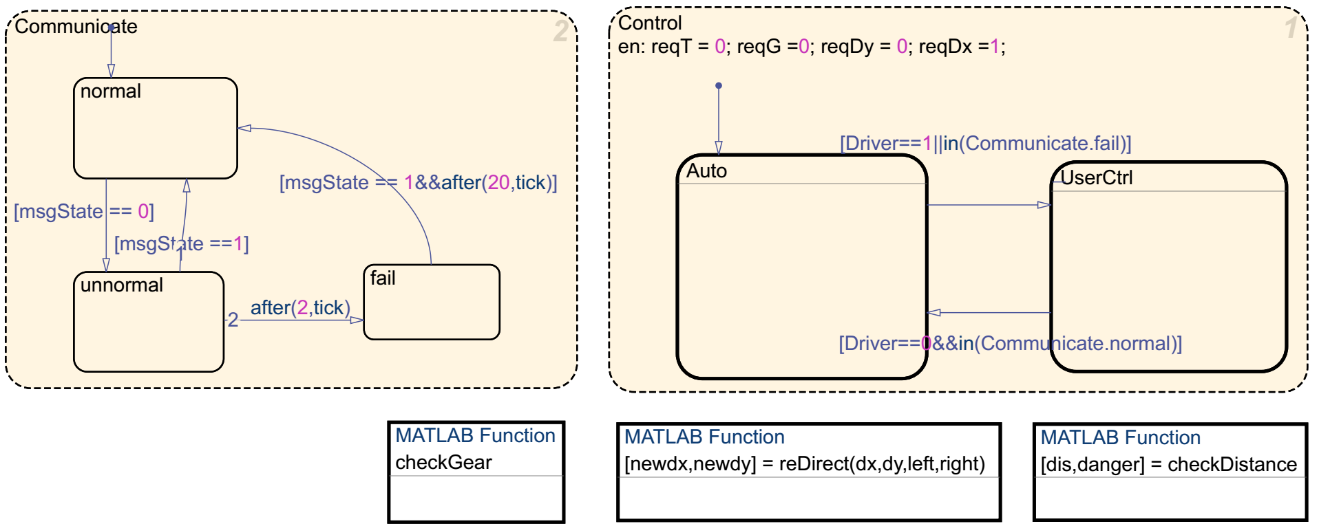
Figure 4.2: Stateflow chart of v1Controller

If the vehicle runs automatically, either leader (shown in Fig.4.3) or follower (shown in Fig.4.4) will be activated according to the absolute positions of the three vehicles. Inside the leader state, there are six superstates turn_right, turn_left, constSpeed, acc, dec and stop together with their child states. The edges represent transitions between the states with the conditions on the edges. Initially, The chart transits to either straight or stop based on the initial speeds of the wheels. The transitions will be taken according to the current speed of the wheels and the value of signType, whose various evaluation represents the different traffic sign. For example, when the vehicle is in constSpeed state and the detected signType is 5 (stop sign is encountered), braking and stop will be activated and brake will become 1 indicating that the velocity of vehicle should be decreased steeply. Whenever the vehicle detects a stop sign, the vehicle will start to brake. If the straight sign is detected (signType is 0), the vehicle will maintain the current state and speed. If the vehicle recognizes a left turn sign, it will first decrease its speed to a low level (less than 30 km/h) and start to turn. After turning left, the vehicle will finally go straight and maintain the speed. turnX and turnY specify the location at which the vehicle turns.

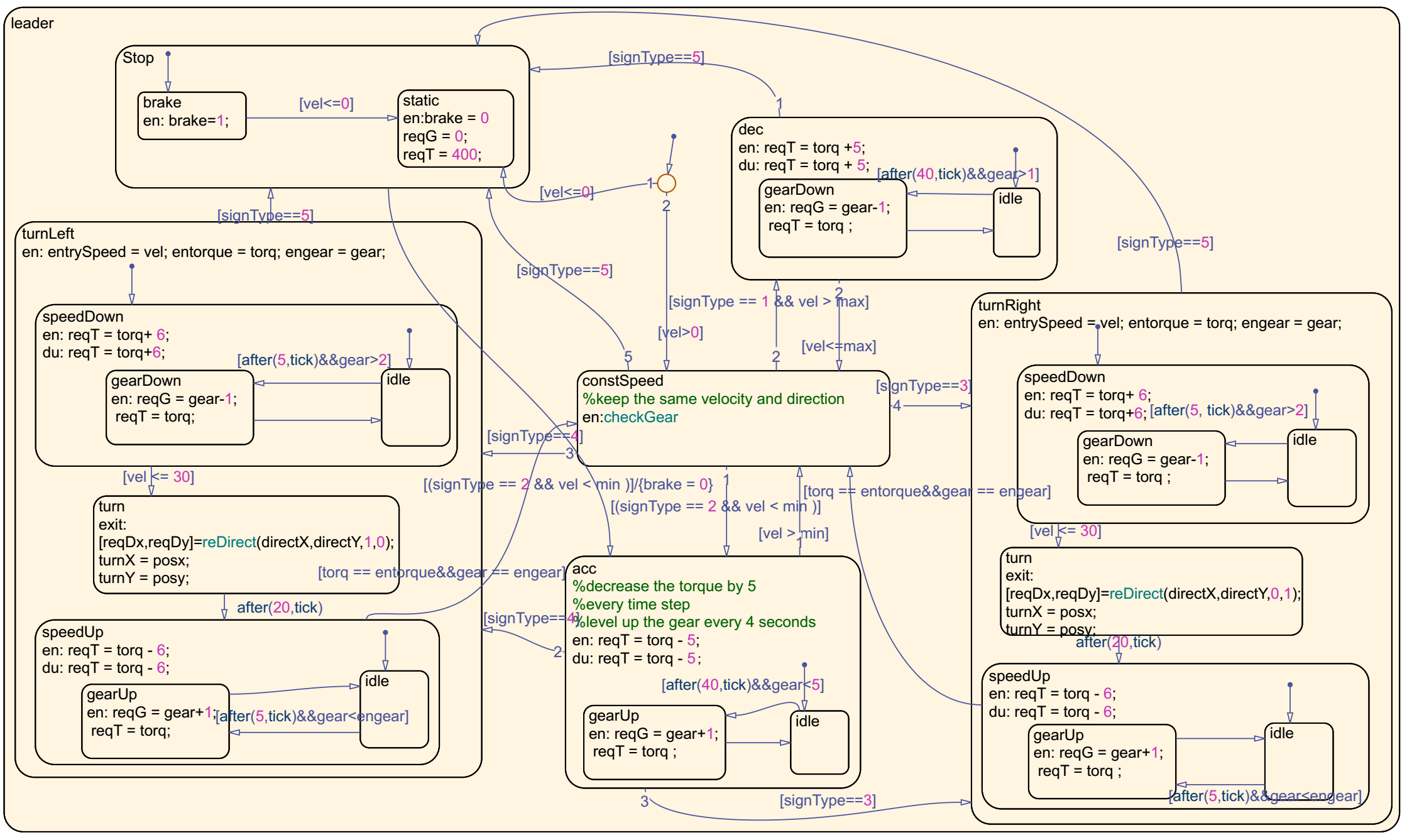
Figure 4.3: leader state in v1Controller

Since a following vehicle should follow the traces and movements of the vehicle in front of it, in follower state, the transitions will be taken once the safety condition is violated, e.g., the distance between the two adjacent vehicles is either larger than 500m or less than the safety distance. As illustrated in turn state on the left of Fig.4.4, when the following vehicle is turning left/right, it will first accelerate to reach to the turning location at which the lead vehicle turns.

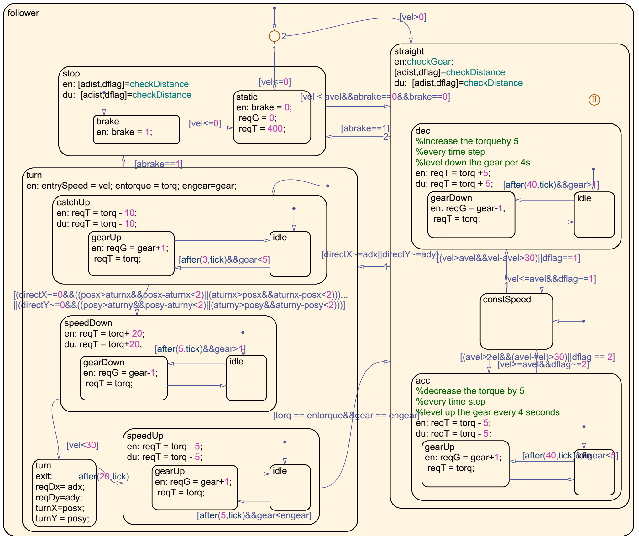
Figure 4.4: follower state in v1Controller

If the vehicle is driven by its driver, userCtrl state (as illustrated in Fig.4.5) will be active. The running mode (stop, turnLeft, turnRight and straight) of the vehicle will be changed based on the driver’s operations. steer represents the steering operation is conducted, i.e., steering to left (steer = 1), right (steer = 2) and straight (steer = 3).

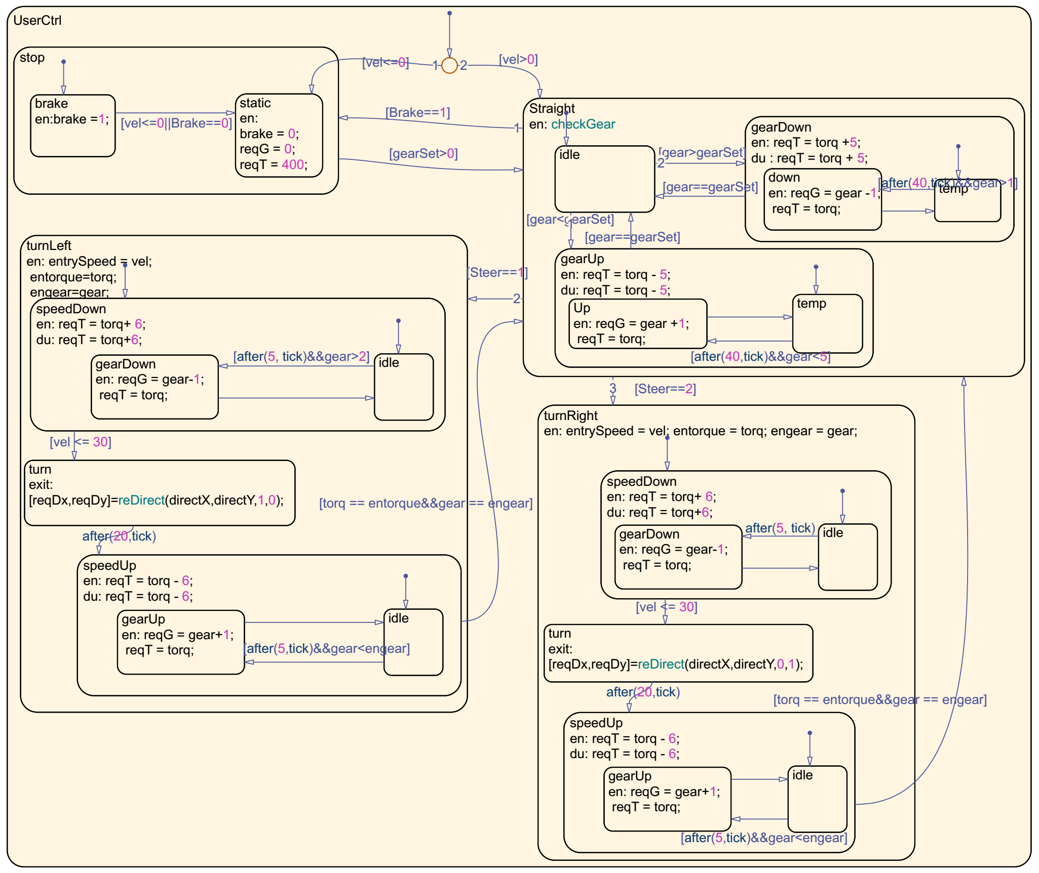
Figure 4.5: userCtrl state in v1Controller

Fig.4.6 illustrates the Simulink and Stateflow model of localEnv, whose functionality is captured in three subsystems: ComDevice is responsible for signal propagation and message receiving; DriverBehavior records the value of signals (gear, steer, brake and DriverState) that represent various operations conducted by the driver; VehicleDynamic specifies the how the velocity and running direction of the vehicle are changed according to the input torque and gear value. In this figure, blocks/entities in green format are employed to model timing constraints, whose modeling process will be explained detailly in the following section.

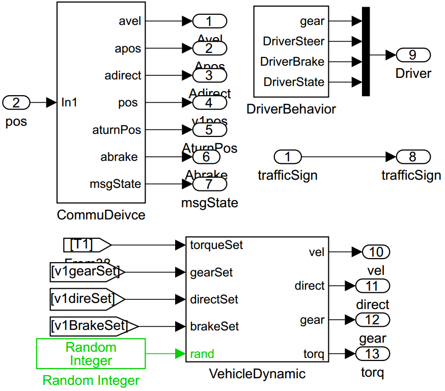
Figure 4.6: Simulink & Stateflow model of localEnv

Fig.4.7 shows the Simulink and Stateflow model of DriverBehavior $f_{p}$. This subsystem obtains inputs from the driver by $\ll$Manual Switch$\gg$ block, which represents a toggle switch where one of its two inputs (1 or 0) will be selected to pass through and become the value of the output.

Figure 4.7: Simulink & Stateflow model of DriverBehavior

Fig.4.8 shows the Simulink and Stateflow model of VehicleDynamic $f_{p}$. In VehicleDynamic subsystem, a $\ll$Look Up Table$\gg$ block maps inputs (gear and torqueSet) to an output value (wheelspeed) by looking up or interpolating the predefined values in a table. $\ll$DataStore$\gg$ block records the energy consumption in the duration of braking.

Figure 4.8: Simulink & Stateflow model of VehicleDynamic

Figure 4.9: Simulink & Stateflow model of ComDevice

4.2 Modeling Timing and Energy Constraints in Simulink/Stateflow

In this section, we investigate how to model timing and energy constraints in S/S. In our previous work, we have shown how those constraints are interpreted in S/S and provided corresponding modeling extensions in S/S. However, the previous modeling extensions contain blocks that are unsupported in SDV, which leads to incompatibility problem. To perform verification of timing and energy constraints in SDV, the modeling extensions are modified to ensure the compatibility.

Sporadic timing constraint is modeled using “after(min, msec)” expression, which returns true after min milliseconds (msec) have elapsed since activation of the associated state. Synchronization timing constraint restricts the time duration among a set of events (i.e., maximum allowed time between the arrival of the event occurrences). We use In1, In2 and In3 (in Fig.4.10(a)) to indicate the arrivals of the three inputs of $f_{p}$. To verify Synchronization constraint, we check whether the interval between occurrences of earliest and latest input event is within tolerance, which is described in Chap. 5.

As shown in Fig.4.10(a), to model Execution timing constraint of an $f_{p}$, a Stateflow chart is used to create a true duration to execute the $f_{p}$. The $\ll$Enable Subsystem$\gg$ ES (representative of $f_{p}$) executes when Exe state is active. t is the Execution constraint applied on the $f_{p}$. id is a monotonically increased value. To ensure the one-to-one correspondence of input and output event, we use two variables, r and s, to represent the value of input and output event respectively. When input event occurs, $f_{p}$ will start to execute and r will be assigned by the value of current id. After t milliseconds, $f_{p}$ finishes execution and s becomes identical with r, which indicates the occurrence of output event.

Fig.4.10(b) shows an EventChain of n $f_{p}$s, we model each $f_{p}$ based on the pattern of Fig.4.10(a). For each $f_{p}$, $r_{i}$ and $s_{i}$ represent the values of input and output event. Hence in this EventChain, r₁ is the value of source event and s_n is the value of target event of End-to-End constraint. To identify the one-to-one correspondence of source and target event, r₁ and s_n should have the same assigned value.

(a) Execution

(b) End-to-End

Figure 4.10: Timing constraints modeling

We consider two types of Periodic timing constraints: cumulative constraint and noncumulative constraint. T and j indicate the period and jitter of Periodic constraint. In Fig.4.11, e(i) denotes the time point of the $i^{th}$ occurrence of a single event e. e${}_{\texttt{i}}$ represents the $i^{th}$ occurrence of event e. Cumulative Periodic constraint limits that the time intervals between any two consecutive occurrences of e (e.g, $\mid$e(2)-e(1)$\mid$ and $\mid$e(3)-e(2)$\mid$) should be within [T-j, T+j]. Noncumulative Periodic constraint limits that e(i) should be within [i*T-j, i*T+j].

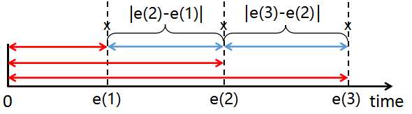
Figure 4.11: Cumulative and Noncumulative constraint

Fig.4.12(a) shows the model of Cumulative Periodic timing constraint of $f_{p}$. The behaviour of $f_{p}$ is modeled in TS (Trigger subsystem) The Stateflow chart generates a signal Trig to trigger TS. rand is a random number within [0, 2*j]. Once $f_{p}$ is triggered, it will be triggered again after T-j+rand ms such that the time interval between any two consecutive triggerings of $f_{p}$ is in [T-j, T+j]. Fig.4.12(b) shows the model of Noncumulative Periodic timing constraint of $f_{p}$ (modeled in TS1). A $\ll$Pulse Generator$\gg$ (PG) generates square waves based on Period and Phase delay parameters. Phase delay specifies the delay before the pulse is generated. PG generates a square wave signal whose Period is T and Phase delay is T-j such that the $i^{th}$ rising edge of the signal arrives at the time point of i*T-j. In the mean time, TS will be triggered to pass rand and $\ll$Delay$\gg$ block delays the rising edges by rand ms s.t. the time point of the $i^{th}$ rising edge will be in [i*T-j, i*T+j].

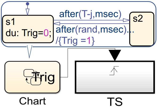
(a) Cumulative

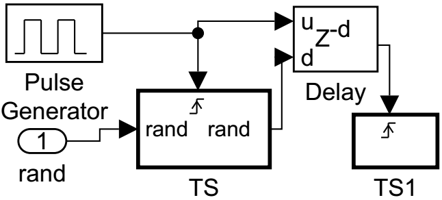
(b) Noncumulative

Figure 4.12: Periodic constraint modeling

Energy constraints are modeled with $\ll$Data Store$\gg$ and integrated Matlab blocks, which calculate and record energy consumption in different modes of a vehicle. According to the various modes of vehicles in CAS, the amount of battery consumed for the mechanical motion of wheels is calculated: $energy$ $=$ $\int_{0}^{t}$ $a*v$ $dx$ where, $t$, $a$, and $v$ denote running time, coefficient reflects an energy rate associated to the current mode of an individual vehicle, and velocity respectively.

Chapter 5 Timing & Energy Requirements Translation in SDV

To enable the verification of the timing and energy requirements illustrated in Chap. 4, we specify timing and energy requirements as LTL formulas and provide the approach to model linear temporal logic (LTL) [11] formulas into proof objective models.

5.1 LTL Properties

An LTL formula usually consists of predicates and propositional connectives, together with temporal operators (e.g. Always, Eventually and Until).

Always p (G p) states that property p always holds along the execution, which is modeled as the proof objective model described in Chap. 2.

Always and Eventually within t time steps: Always p within t time steps, denoted by G${}_{[0,\ t]}$ p, is valid if property p holds over the first t time steps during execution. Eventually p within t time steps, denoted as F${}_{[0,\ t]}$ p, holds if p occurs within the first t time steps during the execution. The model of Always property and Eventually are illustrated on the left and right of Fig.5.1: dur is a signal which is true within the first t time steps. To checks whether p always holds true within the true duration, p is connected to $\ll$Implies$\gg$ block. $\ll$Within Implies$\gg$ block is employed to verify whether p holds for at least one time step within the true duration dur. P block is applied to prove whether the property is satisfied.

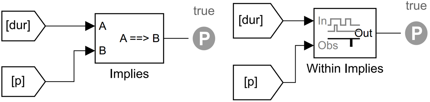
Figure 5.1: Bounded Always and Eventually property

p Until q within t time steps. Denoted as p U_[0,t] q, this property states that p should always hold before q becomes true within the first t time steps during the execution. The satisfaction of this property requires $\varphi_{1}$: q must hold at least one time step within the first t time steps; $\varphi_{2}$: before q holds, p must always be true. This property can be interpreted as: F${}_{[0,\ t]}$ q $\wedge$ G${}_{[0,\ t]}$ ($\neg$q $\implies$ p). The implementation of this property is shown in Fig.5.2: dur has a true duration with length t. First, a $\ll$Within Implies$\gg$ block check whether $\varphi_{1}$: F${}_{[0,\ t]}$ q holds. An $\ll$Extender$\gg$ block is applied to extend the true duration of q to t time steps after q occurs. $\ll$Not$\gg$ block is then employed to capture the true duration of $\neg$q. $\ll$Implies$\gg$ block checks whether “not q implies p” holds. Afterwards, $\ll$And$\gg$ and $\ll$Proof Objective$\gg$ validate whether “$\varphi_{1}$ $\wedge$ $\varphi_{2}$” is always true.

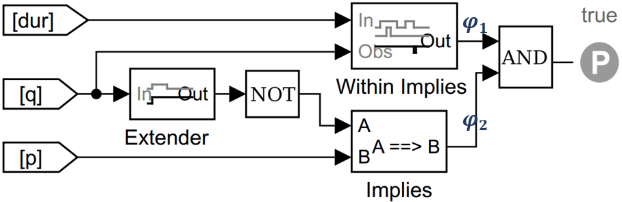
Figure 5.2: p Until q: G (F${}_{[0,\ t]}$ q $\wedge$ ($\neg$q $\implies$ p))

Fig.5.3 illustrates the functional property (R1) which can be specified by using Always and Eventually operators: G_[0,200](auto == true $\wedge$ msgNormal == false) $\implies$ F_[0,200] userCtrl == true. auto (userCtrl) represents whether the vehicle is running automatically (driven manually). msgNormal indicates whether the message is transmitted normally. In Fig.5.3, $\ll$Detector$\gg$ constructs a signal with a 200ms true duration after “auto == true and msg == false” becomes true for 200ms. Within this true duration, “userCtrl == true” should be satisfied at least one time step. To check this, the output signal from $\ll$Detector$\gg$ goes to the $\ll$Goto$\gg$ block tagged with dur. Then it is passed to the corresponding dur tag on the right of Fig.5.1. Similarly, the signal that represents “userCtrl == true” is passed to p tag on the right of Fig.5.1 (the input of $\ll$Within Imply$\gg$) block.

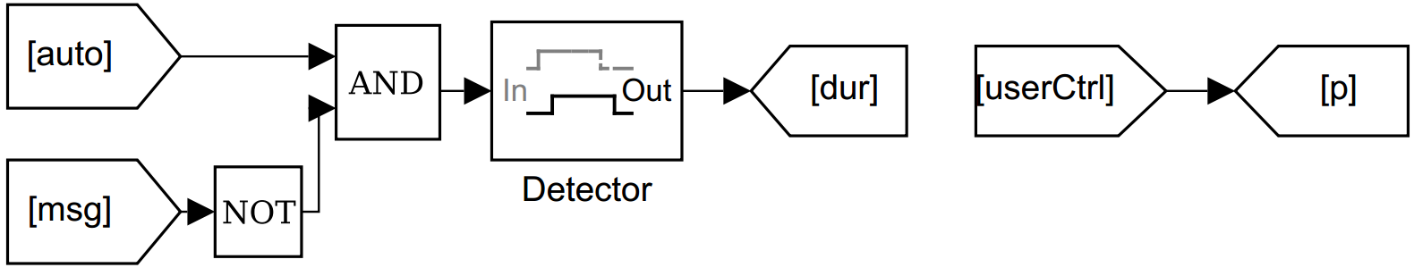
Figure 5.3: Functional Property: When auto is true and msg is false for 200ms, userCtrl should become true within 200ms.

Fig.5.4 illustrates the model of the functional property (R21), which can be specified with Util and Always temporal operators: G (dist12 $<$ safeDis $\implies$ v2.dec == false U_[0,500] v2.dec == true). dist12 is the distance between the lead vehicle (v1) and the following vehicle (v2). safeDis is the required safety distance between them. v2.dec represents whether v2 is decelerating. $\ll$Detector$\gg$ creates a signal with a 500ms true duration after “dist12 $<$ safeDis” becomes true. This signal then goes to the $\ll$From$\gg$ block tagged with dur in Fig.5.2. In this example, p represents the property “v2.dec == false” and q represents “v2.dec == true” as illustrated on the right of Fig.5.4.

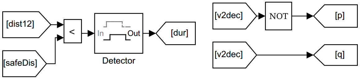
Figure 5.4: Property: If the dis12 is smaller than safeDis, v2dec should be true within 500ms.

5.2 Timing Constraints in SDV

Timing constraints in East-adl are modeled by means of constraints specified on Events and EventChains. A constraint is expressed as a proof objective model in SDV. To proof the correctness of the timing behaviours of Simulink/Stateflow model, we show how to construct the proof objective models for the design model based on the timing constraints. We focus on Synchronization, Execution, End-to-End, Periodic, Sporadic constraints (R27-R46) that are associated to $f_{p}$s in East-adl.

Synchronization timing constraint can be interpreted as: all the input signals should be received within tolerance after the first (earliest) input signal arrives. The model of the timing constraint is shown in Fig.5.5: Assume that there are three input signals of an $f_{p}$. firstIn represents whether the first (earliest) input signal is received. In1, In2 and In3 indicate the arrival of three input signals of $f_{p}$ respectively. $\ll$Extender$\gg$ is employed to construct a true duration with length tolerance from the time step in which firstIn becomes true. Three $\ll$Within Implies$\gg$ block are applied to capture whether In1, In2 and In3 becomes true within the true duration. $\ll$And$\gg$ block then validates whether In1, In2 and In3 all become true within the true duration and pass the output signal to a $\ll$Proof Objective$\gg$ block, which proves whether the constraint is valid.

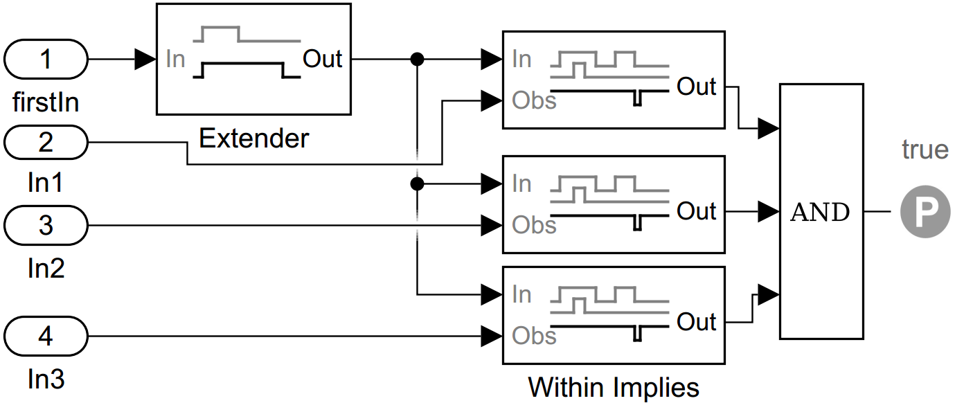
Figure 5.5: Synchronization timing constraint

Execution timing constraint limits that after the input signals are received, the output data should be sent out within upper time steps. The construct of this timing constraint is shown on the left of Fig.5.6 (a): dataIn (dataOut) indicates the input (output) signal received (sent out). $\ll$Extender$\gg$ is applied to construct a true duration with length upper after dataIn becomes true. Afterwards $\ll$Within Implies$\gg$ and $\ll$Proof Objective$\gg$ blocks are used to verify whether the dataOut becomes true within the true duration.

End-to-End timing constraint restricts that after source event occurs, target event should happen within tolerance. The model of this timing constraint is illustrated on the right of Fig.5.6 (b): source and target indicate the source and target event occurs (true) or not (false). $\ll$Extender$\gg$ constructs a true duration with length tolerance after source becomes true. Afterwards $\ll$Within Implies$\gg$ and $\ll$Proof Objective$\gg$ blocks are used to verify whether the target becomes true within the true duration.

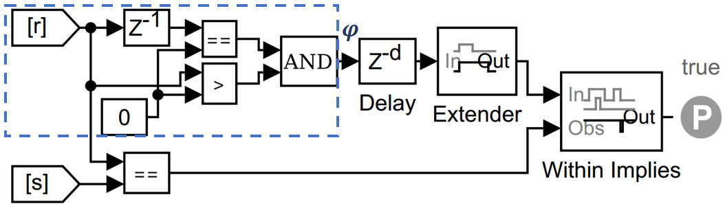
(a) Execution

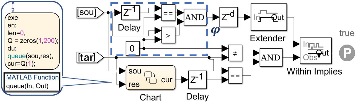
(b) End-to-end

Figure 5.6: Timing constraints translation

Sporadic timing constraint specifies that after the event occurs, the next occurrence should not happen within min time steps. This timing constraint is constructed as the model in Fig.5.7. event indicates the occurrence of an event. $\ll$Detector$\gg$ constructs a true duration with length min after event becomes true. Afterwards, $\ll$Negation$\gg$ (Not) and $\ll$Implies$\gg$ blocks are employed to validate whether p is false over the true duration. At last, $\ll$Proof Objective$\gg$ block checks whether the property is satisfied. Fig.5.8 illustrates an example of sporadic timing constraint (R30), where the constraint is modeled in the dash box. In this example, event is “auto == true”.

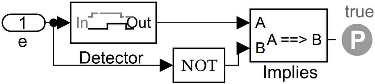
Figure 5.7: Sporadic timing constraint

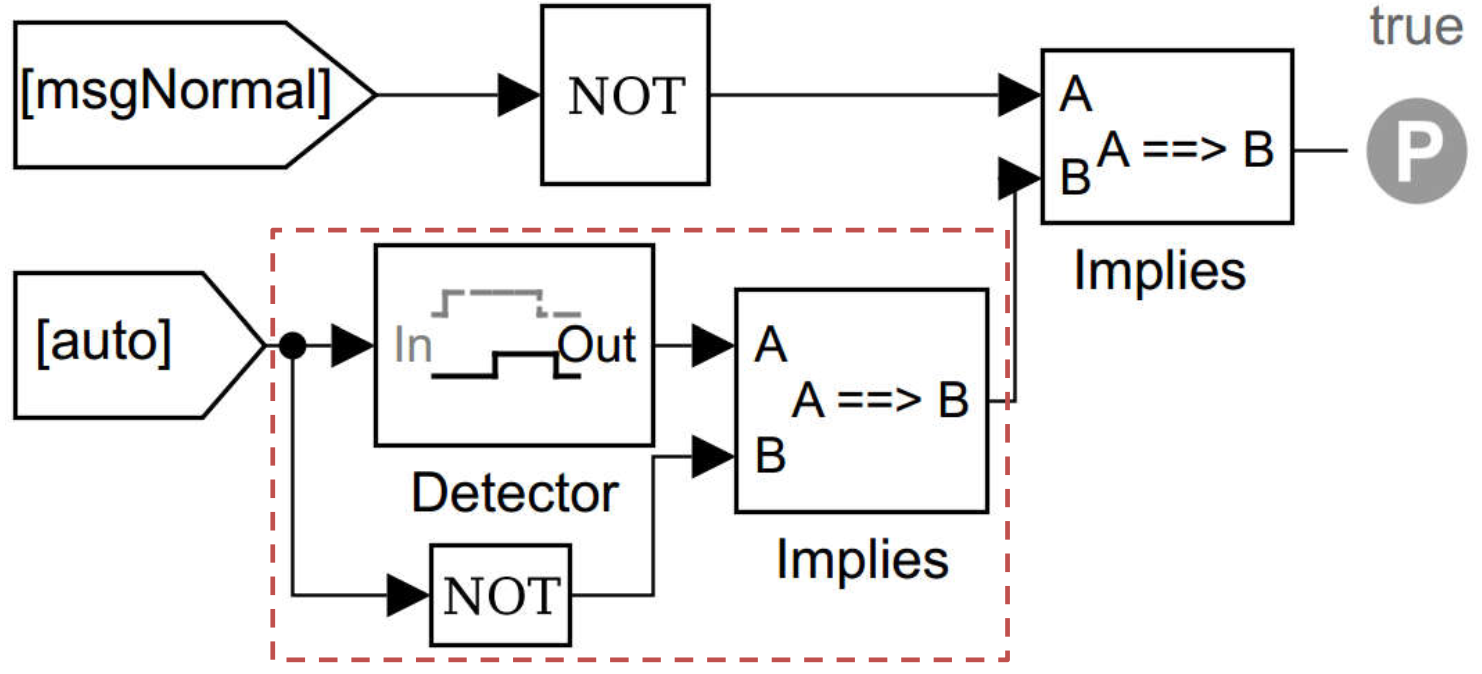
Figure 5.8: R30: if the message transmission is failed (msgNormal == false) when the vehicle runs in auto-mode, for the next 20 seconds, the vehicle should not run automatically, i.e., auto == false

Periodic timing constraint limits a single event $f_{p}$ should occur periodically with period T and jitter j. We consider two types of timing constraints in SDV: 1. Cumulative Periodictiming constraint is modeled as the proof objective model illustrated in Fig.5.9. To verify this property, we check whether $t_{i}+1$ locates in [$t_{i}$+$T$-$j$, $t_{i}$+$T$+$j$]. As shown on the left of Fig.5.9, a $\ll$Delay$\gg$ is to add a T-j delay to the input signal event. As illustrated on the right of Fig.5.9, an $\ll$Extender$\gg$ then generates a true duration with length 2*j such that the range of true duration is [$t_{i}$+$T$-$j$, $t_{i}$+$T$+$j$]. Afterwards, $\ll$Within Implies$\gg$ checks whether event occurs within each true duration. Take R27 as an example, if event firstly occurs at 0.01s, a corresponding true duration [0.05, 0.07] is generated, where the existence of the second occurrence is checked. 2. Noncumulative Periodictiming constraint is constructed with the blocks illustrated in Fig.5.10: a $\ll$Pulse Generator$\gg$ is applied to generate signals (square waves) based on Period, Pulse width, Phase delay parameters (see Fig.5.10). Pulse width is a duty cycle specified as a percentage of Period, i.e., Pulse width = Width/Period. Phase delay specifies the delay before the pulse is generated. $\ll$Convert$\gg$ block is used to transform the signal type from double to boolean. The generated signal and event signal from the input port, are then passed to $\ll$Within Implies$\gg$ block. $\ll$Within Implies$\gg$ checks whether event becomes true within each true duration of the generated signal. Take R27 as an example, the Phase delay is specified as 0.04s, Period is 0.05s and Pulse width is 40%, which is illustrated on the right of Fig.5.10. To satisfy this timing constraint, VehicleDynamic should be triggered within each true duration of the generated signal.

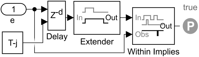
Figure 5.9: Cumulative Periodic Timing Constraint

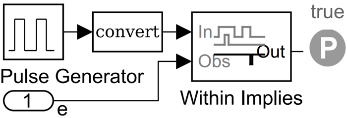
Figure 5.10: Non-cumulative Periodic Timing Constraint

5.3 Energy Constraints in SDV

According to the various modes of vehicles in CAS, the amount of battery consumed for the mechanical motion of wheels is calculated: $energy$ $=$ $\int_{0}^{t}$ $a*v$ $dx$ where, $t$, $a$, and $v$ denote running time, coefficient reflects an energy rate associated to the current mode of an individual vehicle, and wheel speed respectively.

Energy constraint demarcates that the energy consumption on different modes of an individual vehicle is within $[lower,upper]$. It is specified as G$(lower$ $\leqslant$ $energy$ $\wedge$ $energy$ $\leqslant$ $upper)$ and its POM is depicted in Fig. 5.11, where the value of the energy consumption is obtained through $\ll$Data Store Read$\gg$ block and compared with upper and lower.

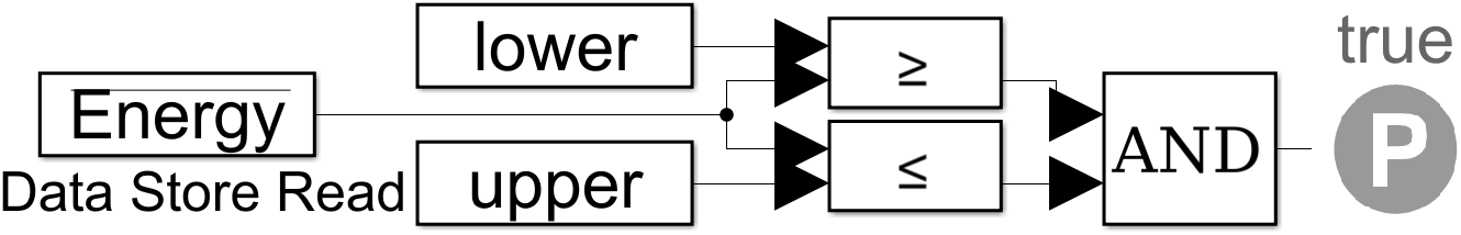
Figure 5.11: Energy constraint

Chapter 6 Modeling Functional Behaviours in Uppaal-smc

We translate the East-adl architectural model illustrated in Fig.3.2 and Simulink/Stateflow model in Fig.4.1 into a networks of STAs in Uppaal-smc. In the model, there are three vehicles receiving the information of traffic signs from cooperative environment CoopEnv $f_{p}$. The functionality traffic sign recognition is modeled as the STA shown in Fig.6.1. The type of traffic signs include stop, left/right turn, straight, minimum/maximum speed limit. The dash line in Fig.6.1 indicates the probabilistic distribution of different traffic signs, i.e., traffic sign occurs randomly with a certain probability. The lead vehicle (v1) will adjust its speed and running direction according to the detected sign types. The two follower vehicles (v2 and v3) will follow the lead vehicle.

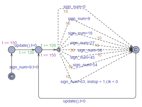
Figure 6.1: STA of SignRecognition

The functionality of the three vehicles are similar. Each vehicle consists of a localEnv $f_{p}$ and a Controller. Each localEnv consists of three $f_{p}$s: ComDevice, VehicleDynamic and DriverBehaviour. ComDevice is modeled in Fig.6.3. The inner behaviour of the vehicle calculating velocity according to the gears and torque is modeled in Fig.6.2. This $f_{p}$ will be triggered to execute periodically with period 50ms and jitter 10ms, i.e., STA of VehicleDynamic will be triggered to update the speed, gear and torque of the vehicle periodically. The computation is implemented as the function speedCal(), which will be called to update the states and valuation of variables whenever the corresponding transition is taken.

Figure 6.2: STA of VehicleDynamic

Fig.6.3(a) captures the behaviour of the sensor sending out signals of position, velocity and direction of vehicle. Fig.6.3(b) models the behaviour of the sensor receiving signals from other vehicles. It receives information (the position, velocity and direction) from the lead vehicle, and detects whether the lead vehicle is braking periodically. The sensor will send out signals/information when the Controller of the vehicle finishes execution.

(a) Sensor of sending signals

(b) Sensor of receiving signals

Figure 6.3: STA for modeling ComDevice

The behaviors of the driver is modeled as the STAs shown in Fig.6.4. Brake Pedal STA represents the behaviors of braking pedal (Fig.6.4(a)). Control status button STA records whether the driver intends to drive the vehicle manually (Fig.6.4(b)). The behaviors of controlling gear and steer is modeled as the STA in Fig.6.4(c) and Fig.6.4(d) respectively. The driver can take charge of the running state of the vehicle by switching the running state to userCtrl mode using Control Button. The driver can control the vehicle by steer (steer the running direction of vehicle), gear (control the speeds of the wheels) and the brake pedal (to stop the vehicle).

(a) Brake Pedal

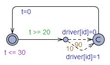
(b) Control Status Button

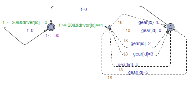
(c) Gear

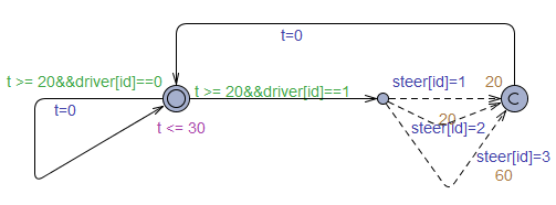
(d) Steer

Figure 6.4: STA for modeling DriverBehaviour

The top view of the Controller modeled in Fig.4.2 is shown in Fig.6.5. The controller gets information from four different sensors. After receiving all input signals, the Controller will decide which state should be activated. Fig.6.6 and Fig.6.8 describe two states that represent auto mode and userCtrl mode of vehicle. If the driver intends to control the vehicle, the Control Button will transit to userCtrl, indicating that the vehicle is driven manually. When Auto location is active, and the vehicle cannot get the information from the ahead vehicle, then userCtrl will be activated automatically.

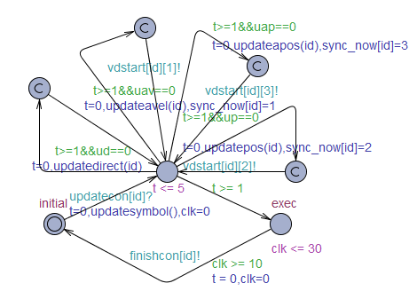
Figure 6.5: STA of Controller

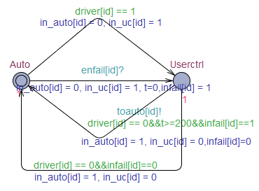
Figure 6.6: STA of Control state

Fig.6.8 describes the behavior that it is of 50% probability that the message transmission is failed. The message state is modeled by STA in Fig.6.7. When the message is missed for 2s, userCtrl mode will be activated.

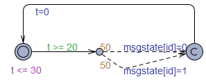
Figure 6.7: STA for deciding whether the message is missing

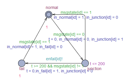
Figure 6.8: STA for modeling Communication state

The behaviour of leader state in the Stateflow chart is captured by STA illustrated in Fig.6.9. The leader gets image information from CoopEnv and changes its running mode according to signType, the current running state and velocity. The substates of leader state is modeled in Fig.6.10.

The inner behaviours of Stop can be captured in Fig.6.10(a). Similarly, Fig.6.10 (b) and Fig.6.10 (c) describe the behaviour of turnLeft, turnRight. Fig.6.11 (a) and Fig.6.11 (b) illustrates the STA of acc and dec state respectively. When the leader vehicle detects a stop sign (signType == 5) and if it is in Auto mode, Stop state in leader STA will be activated and the torque will be set to maximum value (the velocity will be decreased rapidly). When the velocity of the vehicle is less than or equal to 0, it will stop and static state (shown in Fig.6.10) will be active. When a minimum speed limit sign is detected or the driver takes control of the vehicle, the straight state will be active. When the lead vehicle detects a left turn sign and the straight state is active, turnLeft state will be active. The vehicle will first decelerate by decreasing the value of its gear until its velocity is less than or equal to 30km/h. Afterwards, the direction of the vehicle will be changed according to its current direction and the detected traffic sign. After turning, the vehicle will increase its velocity to the original velocity before turning.

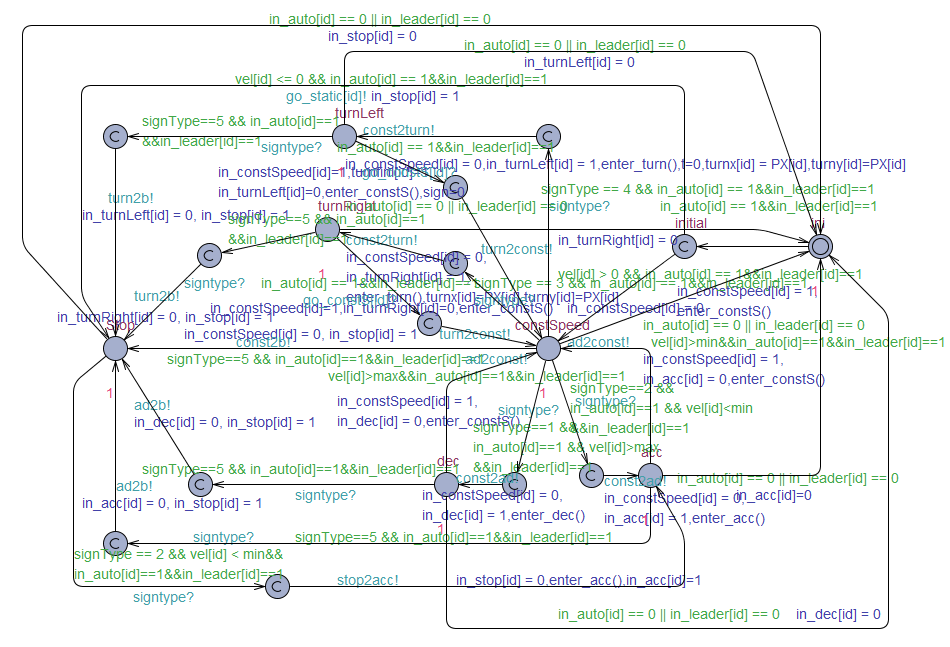
Figure 6.9: STA for modeling leader state

(a) Stop

(b) Turn Left

(c) Turn Right

Figure 6.10: STA for modeling substates of leader state

(a) Accelerate

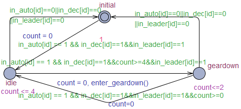
(b) Decelerate

Figure 6.11: STA for modeling substates of leader state

The inner behaviour speedUp and speedDown is modeled in Fig.6.12. When the vehicle is decelerating, the torque (torq) of the vehicle will be increased and the gear (gear) will be decreased. Since the velocity of one vehicle is positively proportional to gear, the velocity will be increased when gear is increased. When the vehicle finishes turning, the torque of the vehicle will be decreased and the gear will be increased to resume to the original velocity.

The inner behaviour of turnLeft state is captured in Fig.6.13. Similarly, when the vehicle detects a turn right sign, it will decelerate until its speed velocity is less than 30km/h. Afterwards, it will turn (its running directions will be changed) and increases its velocity. The acc and dec states (Fig.6.10(d), (e)) represent the states that the vehicle is accelerating or decelerating. When the lead vehicle (v1) detects a minimum speed limit, and the velocity of the vehicle is less than the limit, acc state will be active. The torque of the vehicle will be decreased to order to increase the velocity. In the mean time, the gear of the vehicle will be increased every 40ms until it reaches the maximum value. When the lead vehicle detects a maximum speed limit and the velocity is larger than the limit, it will activate dec state and its velocity will be decreased.

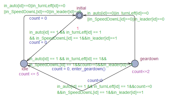
(a) speedDown

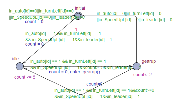
(b) speedUp

Figure 6.12: STA of turnLeft state

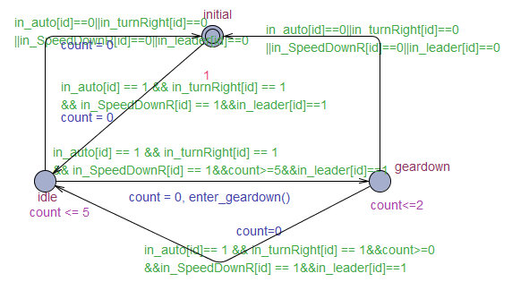
(a) speedDown

(b) speedUp

Figure 6.13: STA of turnRight state

The behaviour of the follower is captured in Fig.6.14. The follow vehicle will decide its behaviour by three super-states: stop, turn and straight, which will be active according to the velocity and running mode of the lead vehicle. It is required to guarantee the distance between the following vehicle and the lead vehicle should be limited in order to ensure the safety. When the follower is in straight state (Fig.6.15(c)), it will always check the distance departing from the leader vehicle by executing checkDistance() function. If the distance is less than the safety distance, then it will activate dec state (Fig.6.15(c)) inside straight state. If the following vehicle is in dec state, which is shown in Fig.6.16(a), it will increase its torque or decrease its gear every 40ms until it reaches 0. If the distance between the following vehicle and the leader vehicle is greater than the safety distance, the vehicle will stop decelerating. When the distance between the following vehicle and the leader vehicle is greater than 500m, in this case, the communication between the two vehicles may be lost. Hence the following vehicle should increase its speed in order to maintain the communication quality.

As presented in Fig.6.16(b), when the vehicle accelerates, it will decrease its torque and increase its gear every 40ms. If the lead vehicle is braking, the follower will activate stop state (shown in Fig.6.15(a)). When the follower stops, it will maintain the safety distance with the lead vehicle. When the follow vehicle detects that its running direction and the running direction of the lead vehicle are different, it will turn left/right in order to keep the same running direction with the lead vehicle. In this case, the following vehicle will first reach the turning point of the lead vehicle (recorded in judgeturnpoint), which is illustrated in Fig.6.14. Similar to lead vehicle, the following vehicle will first decreases the velocity to turn and increase to finish turning. Detailed behaviors of turn state is captured in Fig.6.17.

Figure 6.14: STA of follower state

(a) stop

(b) turn

(c) straight

Figure 6.15: STA of follower state

(a) dec

(b) acc

Figure 6.16: STA for modeling substates of straight state

(a) speedDown

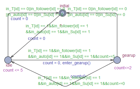
(b) speedUp

Figure 6.17: STA for modeling substates of turn state

If the driver takes control of the vehicle, userCtrl (Fig.6.18) state will be active. The movement of the vehicle will be controlled by the driver. Hence when the driver pressed the brake pedal, stop state in userCtrl will be active. Detailed behaviours of stop state is captured in Fig.6.19(a).

However, when the driver increases the velocity of the vehicle, stop state will transit to straight state. In straight mode,the speed of the vehicle can be increased/decreased by changing the gear (gear up or gear down). As shown in Fig.6.16, the vehicle will adjust its velocity according to the operation by the driver. If the driver steer to left or right, the vehicle will decrease its velocity to turn and increase the velocity to the original velocity after turning (as illustrated in Fig.6.21 and Fig. 6.22).

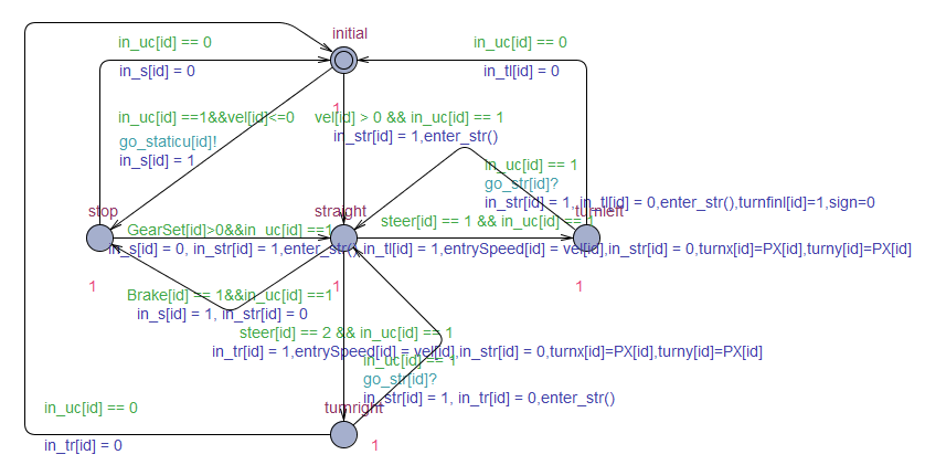
Figure 6.18: STA for modeling userctrl state

(a) stop

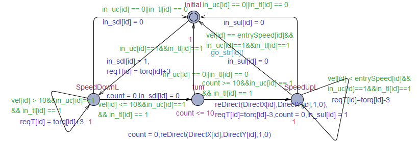
(b) TurnLeft

(c) TurnRight

(d) Straight

Figure 6.19: STA of UserCtrl state

(a) gearUp

(b) gearDown

Figure 6.20: STA for modeling substates of straight state

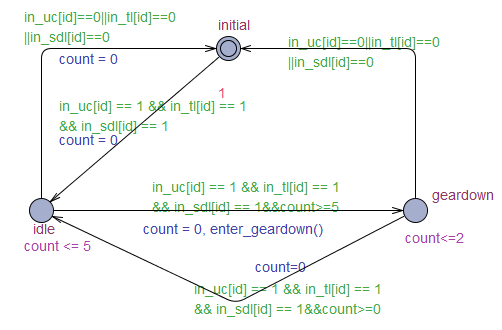
(a) SpeedDownL

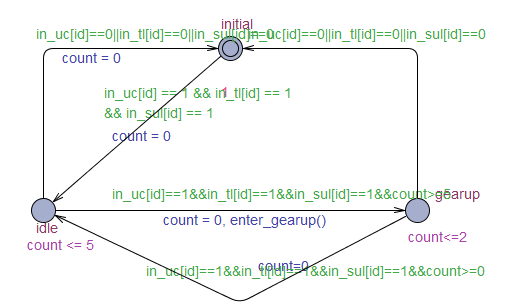
(b) SpeedUpL

Figure 6.21: STA for modeling substates of turnleft state

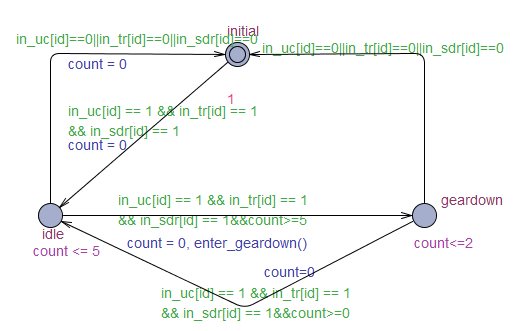
(a) SpeedDownR

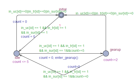
(b) SpeedUpR

Figure 6.22: STA for modeling substates of turnright state

Chapter 7 (Non)-functional Property Translation in Uppaal-smc

In this section, we discuss semantics of the extended Periodic, Sporadic, and Comparison timing constraints (Xtc) with probabilistic parameters according to Tadl[9]. Afterwards, we provide translation of Xtc in Uppaal-smc. Finally, we present how the energy consumption of an individual vehicle in CAS can be modeled in Uppaal-smc.

7.1 Probabilistic Timing Constraints Translation

Xtc that we verified follow the weakly-hard (WH) approach [9], which describes that a bounded number of occurrences among all are allowed to violate the constraints. The semantics of the WH(c,m,k) is that a system behavior must satisfy a given timing constraint c at least m times out of k consecutive occurrences. We use object-oriented notation to define the attributes of occurrences of an event except for Comparison timing constraint, which does not related to any event. $f_{p}$.e refers to an event e of $f_{p}$. we apply e${}_{\texttt{i}}$ and e(i) to represent the $i^{th}$ occurrence of $f_{p}$.e and the time point of $i^{th}$ occurrence respectively.

WH(End-to-End,m,k) limits the interval between the occurrences of $f_{p}$.source and corresponding $f_{p}$.target. For any source${}_{\texttt{i}}$ $\in$ $f_{p}$.source (i $\leq$ $\mid$$f_{p}$.source$\mid$), out of k consecutive occurrences of $f_{p}$.source, i.e., source${}_{\texttt{i}}$ to source${}_{\texttt{i+k}}$, at least m satisfy lower $\leq$ $\mid$target(i)-source(i)$\mid$ $\leq$ upper, where $\mid$target(i)-source(i)$\mid$ denotes the corresponding delay of $f_{p}$.source. We have previously proposed the translation pattern of probabilistic End-to-End constraint, which is applicable for the system where target${}_{\texttt{i}}$ always happens prior to source${}_{\texttt{i+1}}$. To allow the case that source${}_{\texttt{i+1}}$ occurs prior to target${}_{\texttt{i}}$, we model End-to-End constraint as a spawnable STA [5]. As shown in Fig.7.1(a), whenever $f_{p}$.source occurs, Source STA will activate a spawned STA (STA${}_{\texttt{sp}}$(i)) from End-to-End STA (in Fig.7.1(b)). When STA${}_{\texttt{sp}}$(i) is activated, the clock $clk$ starts to count from 0 until target${}_{\texttt{i}}$ occurs. STA${}_{\texttt{sp}}$(i) will judge whether the time interval from source${}_{\texttt{i}}$ to target${}_{\texttt{i}}$ is within the lower and upper bound. According to the judgment, either success or fail location will be activated, representing that the End-to-End constraint is satisfied or not. Afterwards, STA${}_{\texttt{sp}}$(i) will be inactive. To ensure the correspondence of $f_{p}$.source and $f_{p}$.target, if target${}_{\texttt{i}}$ doesn’t occur, STA${}_{\texttt{sp}}$(i) will be inactive when target${}_{\texttt{i+1}}$ occurs. WH(End-to-End,m,k) is specified as: $Pr[bound]$ ($[\ ]$ $\forall$ source${}_{\texttt{i}}$ $\in$ $f_{p}$.source ($\neg$ STA${}_{\texttt{sp}}$(i).$fail$)) $\geqslant$ $P$.

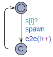
(a) Source

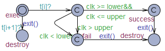
(b) End-to-End (e2e)

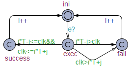
(c) Noncumulative

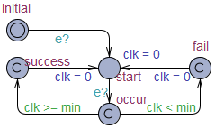
(d) Sporadic

Figure 7.1: Probabilistic Extension of Timing Constraints in Uppaal-smc

WH(Periodic,m,k) limits the period of the successive occurrences of an event including jitter. As our previous work has provide probabilistic extension of Cumu_
Periodic and translation rules to STA, we focus on Noncumu_Periodic. Noncumu_
Periodic: For any e(i) $\in$ $f_{p}$.start, at least m times out of k occurrences, e(i) satisfies: (i*T-jitter $\leq$ e(i) $\leq$ i*T+jitter). In Fig.7.1(c), the STA enforces the $i^{th}$ event event to occur within [i*T-jitter, i*T+jitter]. Initially, STA resets the local clock $clk$ when it counts to $jitter$, which indicates that the time moves backwards by $jitter$ time on the time line. When event happen, STA will judge if $clk$ is within [T-2*jitter, T] and changes its current state to either (success or fail) based on the judgment. Afterwards, the STA will wait at reset till period $T$ and reset $clk$. Finally the STA repeats the calculation. WH(Noncumu_Periodic,m,k) is specified as: $Pr[bound]$ ($[\ ]$ $\neg$ $STA_{Noncumu\_Periodic}.fail$) $\geq$ $P$.

WH(Sporadic,m,k) describes a single event $f_{p}$ that occurs sporadically. For any e(i) $\in$ $f_{p}$.start s.t. its successive occurrence e’(i) starts at e(i), out of k consecutive occurrences e(i), i.e., e(i) to e(i+k), at least m sequences satisfy ($\mid$e’(i)-e(i)$\mid$ $\geq$ min), where min denotes the minimum time interval between consecutive occurrences.In Fig.7.1(d), initially, STA resets the local clock $clk$ when it receives signal $event?$, which indicates the first occurrence of an event. When STA receives $event?$ again, it will judge if $clk$ is larger than $min$ and changes its current state to either (success or fail) based on the judgment. Finally STA reset $clk$ and repeat calculation. WH(Sporadic,m,k) is specified as: $Pr[bound]$ ($[\ ]$ $\neg$ $STA_{Sporadic}.fail$) $\geq$ $P$.

WH(Comparison,m,k) limits the comparison relation (including $<$, $\leq$, $==$, $\geq$ and $>$) among timing expressions, where WH(Comparison,m,k) can be expressed as arithmetic. WH(Comparison,m,k) is defined as: out of k runs, at least m times the comparison relation between TimingExpr1 and TimingExpr2 is satisfied.
WH(Comparison,m,k) is interpreted as: $Pr[bound]$($[]$ TimingExpr1 $\prec$ TimingExpr2) $\geq$ $P$, where $\prec$ $\in$ {$<$, $\leq$, $=$, $\geq$ or $>$}.

7.2 Energy Constraint Estimation

Fig.7.2 shows the stochastic timed automata (STA) that estimates the energy consumption of the Controller of the lead vehicle with extended arithmetic on clocks: total_energy represents the total energy consumption of the Controller of the lead vehicle. Different modes of the vehicle are corresponded to different locations in the STA. As the energy consumption rate for turning right and turning left mode are the same, we combine the two modes into one location in the STA, i.e., turnLeftorRight. Similarly, the acceleration and deceleration mode of the Controller are combined into decoracc. Since the energy consumption rate varies with the running mode of the vehicle, e.g., the energy consumes faster when the vehicle is in braking mode than when the vehicle drives in a constant speed, we define total_energy’ (the rate of total_energy) with ordinary differential equation (ODE) and assign different values to total_energy’ for different locations in the STA. Parameters a, b, c and d are user-defined coefficients to estimate energy consumption of the lead vehicle when it drives in a constant speed, brakes, turns or increases (decreases) its speed respectively. The values of the coefficients indicate the increasing rate of the energy consumption of the Controller and b $>$ d $>$ c $>$ a. The estimation of energy consumption requirement of Controller (R48) will be evaluated in Chap.8.

Figure 7.2: Energy estimation of v1Controller

Also, the four sensors in Fig.3.2(b) will consume energy. As VeDynamicDevice is an imitation of how the velocity of an vehicle can be achieved, its energy consumption is more like the mechanical kinetic energy of the vehicle. While in our case, the velocity and the energy consumption of the vehicle is strongly related to the mode of the vehicle, thus we model the mechanical kinetic energy consumption in Controller (Fig.7.2). The energy of the other three $f_{p}$s, ComDevice, SignRecDevice and VeModeDevice, are modeled in Fig.7.3. In order to simplify calculation, we set constants as the increasing rate of energy consumption of each sensor. When the sensor is working, the energy consumption will increase uniformly. And when the sensors don’t work anymore, the energy consumption will not increase.

(a) Energy of ComDevice

(b) Energy of VeModeDevice

(c) Energy of SignRecDevice

Figure 7.3: Energy constraints on sensors in Uppaal-smc

Chapter 8 Experiment and Verification

Formal verification of functional and non-functional properties are conducted by using SDV and Uppaal-smc. Since SDV only supports a sub-set of blocks in Simulink block library, several blocks need to be replaced from the original model, e.g., look-up table block and random value generator. The proof objective models that specify the functional and non-functional properties are constructed, which are illustrated in the following figures.

Figure 8.1: When v1 runs automatically and if there is no message received by the vehicle for a certain time, the running mode of the vehicle should be changed to manual mode within a certain time: G (G_[0,200] v1.Auto==true $\wedge$ v1.msg == false $\implies$ F_[0,2000] v1.userCtrl == true)

Figure 8.2: When v1 runs automatically with a constant speed, if it detects a stop sign, it should start to brake in 500ms: G (v1.Auto == true $\wedge$ v1.const == true $\wedge$ signType == 5 $\implies$ F_[0,500] v1.stop == true)

Figure 8.3: When the lead vehicle (v1) runs automatically with a constant speed, if it detects left turn sign, it should start to turn left in 200ms: G (v1.auto == true $\wedge$ v1.const == true $\wedge$ signType == 4 $\implies$ F_[0,200] v1.turnLeft == true)

Figure 8.4: If v1 is driven by the driver and it is running with a constant speed, the driver steers to the left, the vehicle will turn left within 200ms: G (v1.userCtrl == true $\wedge$ v1.const == true $\wedge$ v1.steerReq == 1 $\implies$ F_[0,200] v1.turnLeft == true)

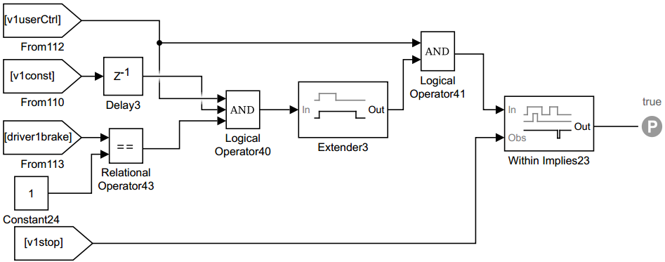
Figure 8.5: If v1 is driven by the driver and it is running at a constant speed, the driver brakes the car, the vehicle will slow down. G: (v1.userCtrl == true $\wedge$ v1.const == true $\wedge$ v1.brakeReq == 2 $\implies$ F_[0,200] v1.brake == true)

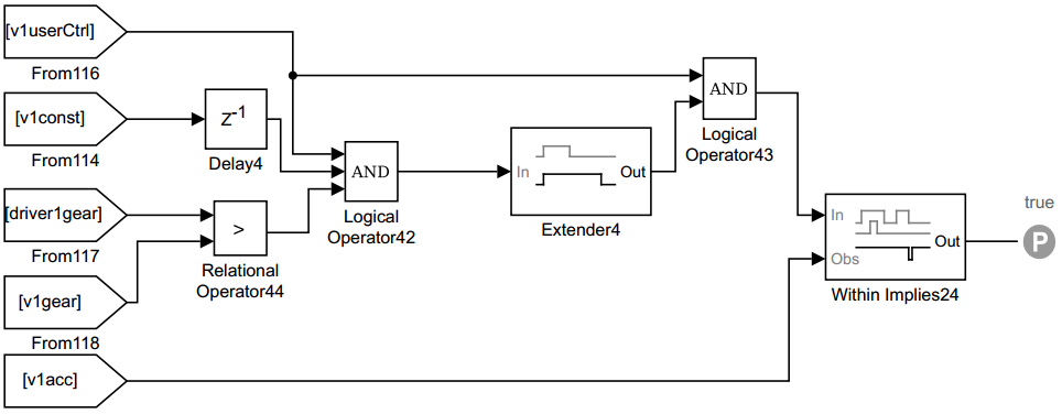
Figure 8.6: When v1 is driven by the driver and it is running at a constant speed, if the driver gears up, the vehicle will accelerate. G (v1.userCtrl == true $\wedge$ v1.const == true $\wedge$ v1.gearReq $>$ v1.gear $\implies$ F_[0,200] v1.acc == true)

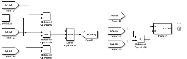
Figure 8.7: When the vehicles are running horizontally, following vehicle should not run ahead of lead vehicle. G (v1.dx == 1 $\wedge$ v2.dx == 1 $\wedge$ v3.dx == 1 $\implies$ v1.x $>$ v2.x)

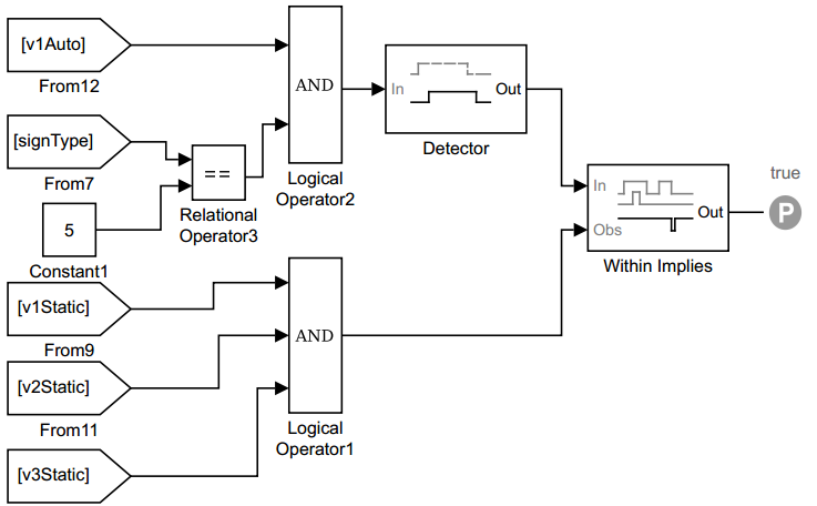
Figure 8.8: When the lead vehicle detects a stop sign, the three vehicles should stop in 5s. G (v1.auto == true $\wedge$ signType == 5 $\implies$ F_[0,5000] v1.static == true $\wedge$ v2.static == true $\wedge$ v3.static==true)

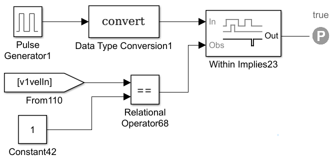
Figure 8.9: Noncumulative Periodic timing constraint: A Periodic acquisition of VehicleDynamic of v1 must be carried out for every 50 ms with a jitter 10 ms. G (v1.velIn == true $\implies$ v1.velIn == false U_{[40, 60]} v1.velIn == true)

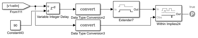
Figure 8.10: Cumulative Periodic timing constraint of R27

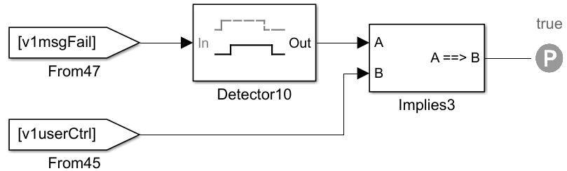
Figure 8.11: Sporadic constraint: After the running mode of the lead vehicle is changed to manual mode because of the failed message transmission, the driver should not change it into auto mode within 20 seconds. G (v1.msgNormal == false $\implies$ v1.auto == false U${}_{[2000,\ \infty]}$) v1.auto == true

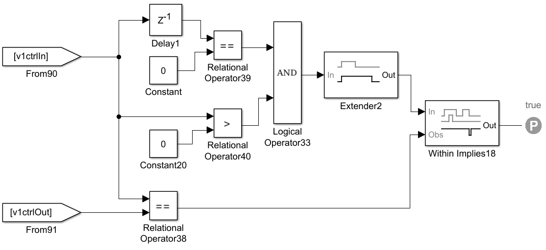
Figure 8.12: An Execution constraint applied on v3Controller, which measured from the inputs ports Avel to output ports gearReq, torqueReq, and brake, should be between 100 ms and 300 ms; G (v3.ctrlIn $\implies$ F_[100,300] v3.ctrlOut)

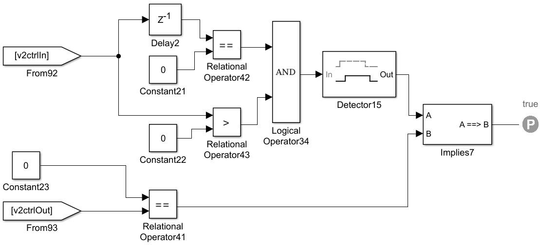
Figure 8.13: An Execution constraint applied on v3Controller, which measured from the inputs ports Avel to output ports gearReq, torqueReq, and brake, should be between 100 ms and 300 ms; G (v3.ctrlIn $\implies$ F_[100,300] v3.ctrlOut)

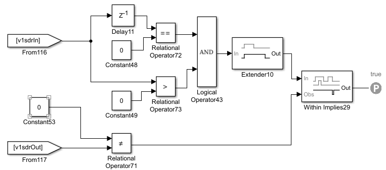
(a) Upper bound

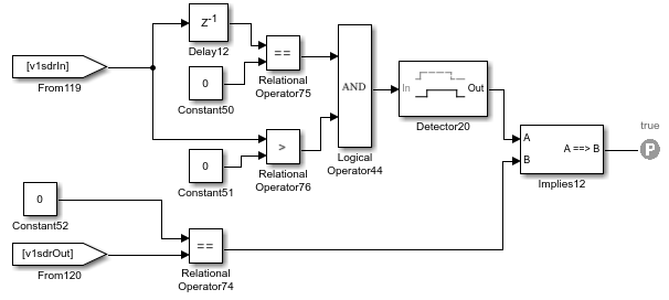
(b) Lower bound

Figure 8.14: An Execution constraint applied on ComDevice of v1, which measured from the inputs ports torqueSet, gearSet and brake to output ports wheelSpeed, direct should be between 100 ms and 150 ms; G (v1.sdrIn $\implies$ F_[100,300] v1.sdrOut

Functional properties of CAS (R1-R26) can be measured using observer STAs. Observer STA describes the time delay between two transitions, i.e., two events. An event can be indicated by a synchronization channel, changes of states or data. Trigger STA represents the events that are represented by changes of states or data. Fig.8.15 shows how functional requirements can be modeled in observer STA. For R1, the observer STA will start to count the elapsed time when communication failure occurs. It stops counting when the driver of this vehicle takes control of the vehicle. An STA is used to indicate the time instant at which the driver takes control of the car (the manual mode is activated). Whenever the user takes control (in_uc[0]==1), a signal will be sent to the STA in Fig.8.15(a) and time counting will be ceased.

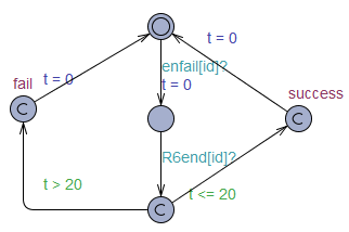
(a) R1

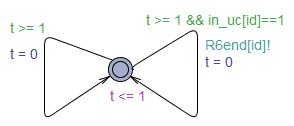
(b) Trigger of R1

Figure 8.15: Observer STA of R1 and its triggering

Verification of timing properties (R27-R50) are done by adapting observer STAs in Fig.8.16. R27-R29 are verified by using the STAs in Fig.8.16(a) and (b), where the VeDynamicDevice is triggered periodly with jitter 10ms. R30-R32 are Sporadic constraints: if communication is missing, the driver should take control of the vehicle for at least 2s (Fig.8.16(c)). The Execution timing constraint of Controller and ComDevice are considered in STAs shown in Fig.8.16(d), (e). The End-to-End constraints measured from the Controller of the lead vehicles to the Controller of the follow vehicles (R39 and R40) can be checked by employing the STAs in Fig.8.16(f). R41-R43 measure the time duration from the Controller of each vehicle receiving signal from the sensors to sendig information to other vehicles (Fig.8.16(g)). The synchronization of the input ports of the Controller can be modeled in STA in Fig.8.16(h).

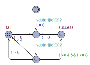
(a) Cumulative Periodic

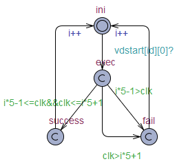
(b) Noncumulative Periodic

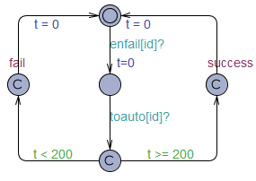
(c) Sporadic

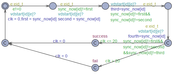
(d) Synchronization

Figure 8.16: Uppaal-smc STAs for timing constraints verification

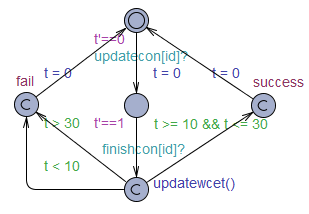
(a) Execution on Controller

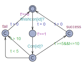
(b) Execution on Sensor

Figure 8.17: Uppaal-smc STAs for End-to-End timing constraints verification

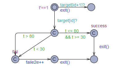
(a) End-to-End between vehicles

(b) End-to-End for one vehicle

Figure 8.18: Uppaal-smc STAs for End-to-End timing constraints verification

Table.LABEL:table_verification_result depicts the verification result of a list of functional (R1-R26) and non-functional (R27-R50) properties. The experiments are performed on a computer with Intel Core i3 CPU and 4GB of RAM. For Periodic timing constraints (R27-R29), results are provided in two categories: cumulative (R27.1, R28.1, R29.1) and non-cumulative (R27.2, R28.2, R29.2). The non-functional properties (R27-R50) are all satisfied in both Uppaal-smc and SDV. The functional properties R1-R22, R25-R26 are established as valid in SDV and are satisfied in Uppaal-smc with confidence greater than 95%, while R23-R24 is invalid in both SDV and Uppaal-smc.

Table 8.1: Logic expression and verification results of the requirements

Req	Type	Expression	Result	Time (min)	Memory (Mb)	CPU (%))
R1	SDV	G (G[0,2000] v1.auto==true $\wedge$ v1.msgNormal==false $\implies$ F[0,200] v1.userCtrl==true)	valid	14.95	1675.47	0.55
	Uppaal-smc	Pr[$\leqslant$3000] ([ ] ($\neg$Commufail(0).fail))	[0.902, 1]	7.61	38.48	22.40
R2	SDV	G (G[0,200] v2.auto==true $\wedge$ v2.msgNormal==false $\implies$ F[0,200] v2.userCtrl==true)	valid	18.45	1782.39	0.29
	Uppaal-smc	Pr[$\leqslant$3000] ([ ] ($\neg$Commufail(1).fail))	[0.902, 1]	6.83	40.49	22.49
R3	SDV	G (G[0,200] v3.auto==true $\wedge$ v3.msgNormal==false $\implies$ F[0,200] v3.userCtrl==true)	valid	26.3	1932.35	0.69
	Uppaal-smc	Pr[$\leqslant$3000] ([ ] ($\neg$Commufail(2).fail))	[0.902, 1]	7.89	42.88	22.62
R4	SDV	G (v1.auto==true $\wedge$ v1.const==true $\wedge$ signType==5 $\implies$ F[0,500] v1.brake==true)	valid	46.8	1964.57	10.25
	Uppaal-smc	Pr[$\leqslant$3000] ([ ] ($\neg$R4TR.fail)) $\geqslant$ 0.95	valid	21.63	39.27	24.75
R5	SDV	G (v1.auto==true $\wedge$ v1.const==true $\wedge$ signType==4 $\implies$ F[0,200] v1.turnLeft==true)	valid	40.08	2072.23	11.21
	Uppaal-smc	Pr[$\leqslant$3000] ([ ] ($\neg$R5TR.fail)) $\geqslant$ 0.95	valid	25.33	39.20	24.52
R6	SDV	G (v1.auto==true $\wedge$ v1.const==true $\wedge$ signType==3 $\implies$ F[0,200] v1.turnRight==true)	valid	40.28	2026.57	6.84
	Uppaal-smc	Pr[$\leqslant$3000] ([ ] ($\neg$R6TR.fail)) $\geqslant$ 0.95	valid	25.67	39.20	24.78
R7	SDV	G (v1.userCtrl==true $\wedge$ v1.const==true $\wedge$ v1.steerReq==1 $\implies$ F[0,200] v1.turnLeft==true)	valid	99.95	2144.16	8.64
	Uppaal-smc	Pr[$\leqslant$3000] ([ ] ($\neg$R7TR.fail)) $\geqslant$ 0.95	valid	27.6	39.10	24.67
R8	SDV	G (v1.userCtrl==true $\wedge$ v1.const==true $\wedge$ v1.steerReq==2 $\implies$ F[0,200] v1.turnRight==true)	valid	157.68	1852.91	1.78
	Uppaal-smc	Pr[$\leqslant$3000] ([ ] ($\neg$R8TR.fail)) $\geqslant$ 0.95	valid	24.48	39.09	24.65
R9	SDV	G (v1.userCtrl==true $\wedge$ v1.const==true $\wedge$ v1.brakeReq==2 $\implies$ F[0,200] v1.brake==true)	valid	80.46	1667	1.46
	Uppaal-smc	Pr[$\leqslant$3000] ([ ] ($\neg$R9TR.fail)) $\geqslant$ 0.95	valid	28.2	39.26	24.63
R10	SDV	G (v1.userCtrl==true $\wedge$ v1.const==true $\wedge$ v1.gearReq$>$v1.gear $\implies$ F[0,200] v1.acc==true)	valid	6.98	1882.97	2.95
	Uppaal-smc	Pr[$\leqslant$3000] ([ ] ($\neg$R10TR.fail)) $\geqslant$ 0.95	valid	29.16	38.92	24.52
R11	SDV	G (v1.userCtrl==true $\wedge$ v1.const==true $\wedge$ v1.gearReq$<$v1.gear $\implies$ F[0,200] v1.dec==true)	valid	259.98	1430	1.85
	Uppaal-smc	Pr[$\leqslant$3000] ([ ] ($\neg$R11TR.fail)) $\geqslant$ 0.95	valid	29.03	39.24	24.57

Req	Type	Expression	Result	Time (min)	Memory (Mb)	CPU (%))
R12	SDV	G (v1.dx==1 $\wedge$ v2.dx==1 $\wedge$ v3.dx==1 $\implies$ v1.x$>$v2.x)	valid	14.02	1320	3.65
	Uppaal-smc	Pr[$\leqslant$3000]([ ] (dx[0]==1 $\wedge$ dy[0]==0 $\wedge$ dx[1]==1 $\wedge$ dy[1]==0 $\wedge$ (in_Str[0] $\vee$ in_dec[0] $\vee$in_str[0]$\vee$in_acc[0]$\vee$in_constSpeed[0]) $\wedge$ (in_Str[1]$\vee$in_str[1]) $\implies$ x[0] $>$ x[1])) $\geqslant$ 0.95	valid	13.27	57.06	24.31
R13	SDV	G (v1.dx==1 $\wedge$ v2.dx==1 $\wedge$ v3.dx==1 $\implies$ v2.x$>$v3.x)	valid	35.37	2085	3.05
	Uppaal-smc	Pr[$\leqslant$3000]([ ] (dx[1]==1 $\wedge$ dy[1]==0 $\wedge$ dx[2]==1 $\wedge$ dy[2]==0 $\wedge$ (in_Str[1] $\vee$ in_dec[1] $\vee$in_str[1]$\vee$in_acc[1]$\vee$in_constSpeed[1]) $\wedge$ (in_Str[2]$\vee$in_str[2]) $\implies$ x[1] $>$ x[2])) $\geqslant$ 0.95	valid	11.43	55.67	24.42
R14	SDV	G ( v1auto $\wedge$ signType==5 $\implies$ F[0,5000] (v1static $\wedge$ v2static $\wedge$ v3static) )	valid	4.67	1903	4.91
	Uppaal-smc	Pr[$\leqslant$3000] ([ ] ($\neg$allstop.fail)) $\geqslant$ 0.95	valid	20.28	52.47	23.10
R15	SDV	G (v1.const==true $\wedge$ v2.const==true $\wedge$ v1.vel$>$v2.vel $\implies$ F[0,200] v2.acc==true)	valid	5.10	2095	4.20
	Uppaal-smc	Pr[$\leqslant$3000] ([ ] ($\neg$acc(1).fail)) $\geqslant$ 0.95	valid	21.52	43.68	22.43
R16	SDV	G (v2.const==true $\wedge$ v3.const==true $\wedge$ v2.vel$>$v3.vel $\implies$ F[0,200] v3.acc==true)	valid	0.15	2038	38.76
	Uppaal-smc	Pr[$\leqslant$3000] ([ ] ($\neg$acc(2).fail)) $\geqslant$ 0.95	valid	19.43	40.46	23.21
R17	SDV	G (v1.const==true $\wedge$ v2.const==true $\wedge$ v1.vel$<$v2.vel $\implies$ F[0,200] v2.dec==true)	valid	0.15	1963	23.04
	Uppaal-smc	Pr[$\leqslant$3000] ([ ] ($\neg$R17TR.fail)) $\geqslant$ 0.95	valid	27.3	39.10	24.60
R18	SDV	G (v2.const==true $\wedge$ v3.const==true $\wedge$ v2.vel$<$v3.vel $\implies$ F[0,200] v3.dec==true)	valid	11.52	2026	3.99
	Uppaal-smc	Pr[$\leqslant$3000] ([ ] ($\neg$R18TR.fail)) $\geqslant$ 0.95	valid	26.89	39.07	24.73
R19	SDV	G (v1.const==true $\wedge$ v2.const==true $\wedge$ dist12$>$500 $\implies$ v2.acc==true	valid	0.04	1961	4.38
	Uppaal-smc	Pr[$\leqslant$3000] ([ ] ($\neg$R19TR.fail)) $\geqslant$ 0.95	valid	27.2	39.16	24.84
R20	SDV	G (v1.const==true $\wedge$ v2.const==true $\wedge$ dist12$>$500$\implies$ v3.acc==true	valid	0.01	1961	4.38
	Uppaal-smc	Pr[$\leqslant$3000] ([ ] ($\neg$R20TR.fail)) $\geqslant$ 0.95	valid	26.53	38.92	24.65
R21	SDV	G (v1.const==true $\wedge$ v2.const==true $\wedge$ dist12$<$safeDis $\implies$ v2.dec==true	valid	11.13	2054	4.09
	Uppaal-smc	Pr[$\leqslant$3000] ([ ] ($\neg$dec(1).fail)) $\geqslant$ 0.95	valid	22.1	43.23	22.60
R22	SDV	G (v2.const==true $\wedge$ v3.const==true $\wedge$ dist23$<$safeDis$\implies$ v3.dec==true	valid	0.03	2234	3.92
	Uppaal-smc	Pr[$\leqslant$3000] ([ ] ($\neg$dec(1).fail)) $\geqslant$ 0.95	valid	20.59	43.27	22.81

Req	Type	Expression	Result	Time (min)	Memory (Mb)	CPU (%))
R23	SDV	G (v1TurnLeft $\implies$ F[0,5000] RunInSameLine)	valid	15.49	1492.96	1.82
	Uppaal-smc	Pr[$\leqslant$3000] ([ ] $\neg$turnleftTime12.fail)$\geqslant$ 0.95	valid	40.93	42.46	24.79
R24	SDV	G(v2TurnLeft $\implies$ F[0,5000] RunInSameLine)	valid	1.10	1918	3.48
	Uppaal-smc	Pr[$\leqslant$3000] ([ ] $\neg$turnleftTime23.fail)$\geqslant$ 0.95	valid	42.71	47.23	23.80
R25	SDV	G (v1.turnRight==true $\implies$ F[0,5000] v1.turnRight==false $\wedge$ v2.turnRight==false $\wedge$ v1.x==v2.x $\vee$ v1.y==v2.y)	valid	0.31	1930	2.02
	Uppaal-smc	Pr[$\leqslant$3000] ([ ] $\neg$turnrightTime23.fail)$\geqslant$ 0.95	valid	39.13	55.11	24.63
R26	SDV	G (v2.turnRight==true $\implies$ F[0,5000] v2.turnRight==false $\wedge$ v3.turnRight==false $\wedge$ v2.x==v3.x $\vee$ v2.y==v3.y)	valid	31.26	2253	3.86
	Uppaal-smc	Pr[$\leqslant$3000] ([ ] $\neg$turnrightTime23.fail)$\geqslant$ 0.95	valid	40.24	56.20	24.89
R27.1	SDV	G (velIn==1 $\implies$ F[40, 60] velIn==1)	valid	28.4	1642	6.51
	Uppaal-smc	Pr[$\leqslant$3000] ([ ] $\neg$VehicleDynamic(0)cumulative.fail)$\geqslant$ 0.95	valid	7.18	51.57	24.64
R27.2	SDV	G (periodpre==0 $\wedge$ period==1 $\implies$ F[0,20] velIn)	valid	8.42	1819.24	1.22
	Uppaal-smc	Pr[$\leqslant$3000] ([ ] $\neg$VehicleDynamic(0)noncumulative.fail)$\geqslant$ 0.95	valid	9.17	51.19	23.25
R28.1	SDV	G (vel2In==1 $\implies$ F[40, 60] vel2In==1)	valid	0.71	1285	0.5
	Uppaal-smc	Pr[$\leqslant$3000] ([ ] $\neg$VehicleDynamic(1)cumulative.fail)$\geqslant$ 0.95	valid	7.28	42.70	24.65
R28.2	SDV	G (p2pre==0 $\wedge$ p2==1 $\implies$ F[0, 20] vel2In)	valid	10.98	2002.17	8.10
	Uppaal-smc	Pr[$\leqslant$3000] ([ ] $\neg$VehicleDynamic(1)noncumulative.fail)$\geqslant$ 0.95	valid	5.6	51.79	24.66
R29.1	SDV	G (vel3In==1 $\implies$ F[40, 60] vel2In==1)	valid	0.65	54.69	8.3
	Uppaal-smc	Pr[$\leqslant$3000] ([ ] $\neg$VehicleDynamic(2)cumulative.fail)$\geqslant$ 0.95	valid	7.23	42.70	24.69
R29.2	SDV	G (p3pre==0 $\wedge$ p3==1 $\implies$ F[0, 20] vel3In)	valid	6.97	2084	8.30
	Uppaal-smc	Pr[$\leqslant$3000] ([ ] $\neg$VehicleDynamic(2)noncumulative.fail)$\geqslant$ 0.95	valid	6.13	51.79	24.49
R30	SDV	G ($\neg$msgNormal $\implies$ $\neg$autoU[2000,∞] auto==true)	valid	4h	1588.14	7.27
	Uppaal-smc	Pr[$\leqslant$3000] ([ ] ($\neg$sporadic(0).fail)) $\geqslant$ 0.95	valid	0.001	30.96	0.9
R31	SDV	G ($\neg$msgNormal2 $\implies$ $\neg$auto2U[2000,∞] auto2==true)	valid	49.15	2253	38.85
	Uppaal-smc	Pr[$\leqslant$3000] ([ ] ($\neg$sporadic(1).fail)) $\geqslant$ 0.95	valid	0.002	30.96	1.2
R32	SDV	G ($\neg$msgNormal $\implies$ $\neg$auto3U[2000,∞] auto3==true)	valid	59.15	2125	36.40
	Uppaal-smc	Pr[$\leqslant$3000] ([ ] ($\neg$sporadic(2).fail)) $\geqslant$ 0.95	valid	23:03	1167.54	22.24
R33	SDV	G (rpre==0 $\wedge$ r$>$0 $\implies$ F[100,300] s==r)	valid	19.7	1661	7.31
	Uppaal-smc	Pr[$\leqslant$3000] ([ ] ($\neg$v1Controllerexecution.fail)) $\geqslant$ 0.95	valid	7.7	51.67	24.71
R34	SDV	G (r2pre==0 $\wedge$ r2$>$0 $\implies$ F[100,300] s2==r2)	valid	1.38	1493	3.63
	Uppaal-smc	Pr[$\leqslant$3000] ([ ] ($\neg$v2Controllerexecution.fail)) $\geqslant$ 0.95	valid	6.5	42.61	24.72
R35	SDV	G (r3pre==0 $\wedge$ r3$>$0 $\implies$ F[100,300] s3==r3)	valid	1.08	1551	20.3
	Uppaal-smc	Pr[$\leqslant$3000] ([ ] ($\neg$v3Controllerexecution.fail)) $\geqslant$ 0.95	valid	7.12	43.24	24.79
R36	SDV	G (rcdpre==0 $\wedge$ rcd$>$0 $\implies$ F[50,100] scd==rcd)	valid	1.83	1533.81	1.49
	Uppaal-smc	Pr[$\leqslant$3000] ([ ] ($\neg$sensor1execution.fail)) $\geqslant$ 0.95	valid	7.47	43.24	24.97

Req	Type	Expression	Result	Time (min)	Memory (Mb)	CPU (%))
R37	SDV	G (rcd2pre==0 $\wedge$ rcd2$>$0 $\implies$ F[50,100] scd2==rcd2)	valid	1.23	12.69	8.07
	Uppaal-smc	Pr[$\leqslant$3000] ([ ] ($\neg$sensor2execution.fail)) $\geqslant$ 0.95	valid	7.03	42.72	24.63
R38	SDV	G (rcd3pre==0 $\wedge$ rcd3$>$0 $\implies$ F[50, 100] scd3==rcd3)	valid	2.26	1515.98	3.41
	Uppaal-smc	Pr[$\leqslant$3000] ([ ] ($\neg$sensor3execution.fail)) $\geqslant$ 0.95	valid	9.91	35.12	24.56
R39	SDV	G (sou1pre==0 $\wedge$ sou2$>$0 $\implies$ (F[300,700] tar1==cur1 $\wedge$ tar1$\neq$0))	valid	30.01	1718.32	3.78
	Uppaal-smc	Pr[$\leqslant$3000] ([ ] forall (e:endtoend) ($\neg$e.fail)) $\geqslant$ 0.95	valid	5.15	39.38	24.54
R40	SDV	G (sou2pre==0 $\wedge$ sou2$>$0 $\implies$ (F[300,700] tar2==cur2 $\wedge$ tar2$\neq$0))	valid	10.08	1204.86	5.96
	Uppaal-smc	Pr[$\leqslant$3000] ([ ] forall (e:endtoend2) ($\neg$e.fail)) $\geqslant$ 0.95	valid	6.27	42.56	24.68
R41	SDV	G(v1.const==true $\wedge$ v2.const==true $\wedge$ dist12$>$500$\implies$ v2.acc==true	valid	0.04	1961	4.38
	Uppaal-smc	Pr[$\leqslant$3000] ([ ] ($\neg$execv1.fail)) $\geqslant$ 0.95	valid	7.28	42.70	24.76
R42	SDV	G(v1.const==true $\wedge$ v2.const==true $\wedge$ dist12$>$500$\implies$ v3.acc==true	valid	0.01	1961	4.38
	Uppaal-smc	Pr[$\leqslant$3000] ([ ] ($\neg$execv2.fail)) $\geqslant$ 0.95	valid	7.47	42.70	24.67
R43	SDV	G(v2.const==true $\wedge$ v3.const==true $\wedge$ dist23$<$safeDis$\implies$ v3.dec==true	valid	0.03	2234	3.92
	Uppaal-smc	Pr[$\leqslant$3000] ([ ] ($\neg$execv3.fail)) $\geqslant$ 0.95	valid	7.33	42.70	24.77
R44	SDV	G ($\neg$ rpre==0 $\wedge$ r$>$0 $\implies$ F[0,200] posIn $\wedge$ F[0,200] AposIn $\wedge$ F[0,200] velIn $\wedge$ F[0,200] AvelIn)	valid	32.53	36.51	15.31
	Uppaal-smc	Pr[$\leqslant$3000] ([ ] $\neg$v1Controllersynchronization.fail)) $\geqslant$ 0.95	valid	5.98	50.84	24.51
R45	SDV	G ($\neg$ r2pre==0 $\wedge$ r2$>$0 $\implies$ F[0,200] posIn2 $\wedge$ F[0,200] AposIn2 $\wedge$ F[0,200] velIn2 $\wedge$ F[0,200] AvelIn2)	valid	105.75	1197.67	6.56
	Uppaal-smc	Pr[$\leqslant$3000] ([ ] $\neg$v2Controllersynchronization.fail)) $\geqslant$ 0.95	valid	7.17	42.37	24.74
R46	SDV	G ($\neg$ r3pre==0 $\wedge$ r3$>$0 $\implies$ F[0,200] posIn3 $\wedge$ F[0,200] AposIn3 $\wedge$ F[0,200] velIn3 $\wedge$ F[0,200] AvelIn3)	valid	1.04	1249.30	4.3
	Uppaal-smc	Pr[$\leqslant$3000] ([ ] $\neg$v3Controllersynchronization.fail)) $\geqslant$ 0.95	valid	7.33	42.37	24.52
R47	SDV	G (etcon1==wcon1 $\wedge$ etcon2==wcon2 $\wedge$ etsen1==wsen1 $\wedge$ etsen2==wsen2 $\implies$ wcon1 + wcon2 + wsen1 + wsen2 $\geqslant$ EndtoEnd)	valid	31.26	2253	38.86
	Uppaal-smc	Pr[$\leqslant$3000]($<$ $>$ $\neg$(etcon1==wcon1 $\wedge$ etcon2==wcon2 $\wedge$ etsen1==wsen1 $\wedge$ etsen2==wsen2 $\implies$ wcon1 + wcon2 + wsen1 + wsen2 $\geqslant$ EndtoEnd) $\leqslant$ 0.05	valid	165.65	175.24	23.53
R48	SDV	G (BrakeEnergy $<$ 30000)	valid	32.53	36.51	1.31
	SMC	E[$\leqslant$3000;100] (max: energy.braking_energy)	7944$\pm$1172	8.7	51.44	24.58
	SMC	simulate 100 [$\leqslant$3000] (total_energy)	valid	7.67	45.50	24.63
R49	SDV	G (ConEnergy $\leqslant$ 30)	valid	18.05	1000.8	2.05
	Uppaal-smc	Pr[$\leqslant$3000] ([ ] energy_con $\leqslant$ 30)) $\geqslant$ 0.95	valid	18.05	1000.8	0.9
R50	SDV	G (CDEnergy $\leqslant$ 5)	valid	31.26	2253	38.86
	Uppaal-smc	Pr[$\leqslant$3000] ([ ] energy_sen $\leqslant$ 5)) $\geqslant$ 0.95	valid	20.2	80.9	24.02

The invalid property R23 is identified using SDV and Uppaal-smc. The counter-examples (CE) generated by SDV is shown in Fig.8.19. We perform the simulation in Uppaal-smc to obtain the error trace of CE, which is illustrated in Fig.8.20. DirectX and DirectY represent the directions of the three vehicles and posx and posy indicate the position of the three vehicles. After analyzing CE, the cause of errors was found: After the lead vehicle turns left, the following vehicle begins to turn left after it detects that the running direction of the lead vehicle is changed. The two vehicles turn left at different locations. We modify SDV and Uppaal-smc models according to the CE: a turning location where the lead vehicle turns is recorded and sent to the following vehicle. Hence all the following vehicles should turn at the same turning location to ensure that the three vehicles are still in a lane after turning. After the refinement, R23 and R24 are satisfied in both SDV and Uppaal-smc.

(a) signType

(b) Vehicles’ position

Figure 8.19: CE in SDV: In (b), leadVe.y equals to followVe.y) from 0 to 8s, which indicates that the two vehicles run in the same lane. In (a), signType becomes “turn left (4)” at 8s and the lead vehicle begins to turn left. However, the following vehicle turns left at a different location (leadVe.x is not equal to followVe.x at 9s). Hence, the “x” is unequal after turning, which means that the two vehicles run on different lanes. Thus R23 and R24 is violated.

Figure 8.20: CE in SMC: At the beginning, three vehicles run towards direction (1,0). The three values of posy are the same, which indicates that the three vehicles are in the same lane. After a left turn sign is detected, the lead vehicle starts to turn left. Since the first follower turns left at (184, 0) and the second turns left at (157, 0), the three values of posx are not equal after turning, which indicates the three vehicle are not running in the same lane. Thus R5 is violated.

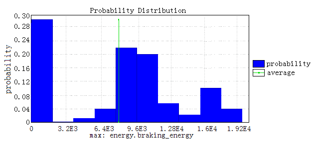
Figure 8.21: Probabilistic distribution of the expected energy consumption

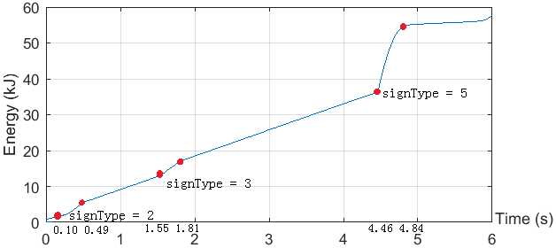
Figure 8.22: Total energy consumption estimation of the lead vehicle

Probability Estimation query is applied on R1-R47, R49-R50, indicating that the property can be verified as valid within [0.902, 1]. For estimate the maximum energy consumption for braking the vehicles (R48), we adapt Expected value query and generate probability distribution diagram (Fig.8.21) of the expected energy consumption. It illustrates that the average of energy consumption is approx. 7944J and the expected energy consumption is always less than 30kJ. The total energy of the lead vehicle is estimated with Simulation query for 100 times within 300 time units. Fig.8.22 shows the result of one time simulation. At the beginning, the lead vehicle runs at constant speed, hence the total energy consumption increases constantly. When it recognizes the minimum speed limit sign (signType = 2), the vehicle starts to accelerate thus energy is consumed faster. The total energy then increases constantly with slight fluctuation due to energy consumption of the sensor and the camera. When the vehicle recognizes a turn right sign (signType = 3), it turns right from 1.55s to 1.88s, during which the energy is consumed faster than when the vehicle is running constantly. The vehicle finally recognizes a stop sign (signType = 5) at 4.46s and stops at 4.84s. The total energy consumed during braking is 18.33kJ, which is less than 30kJ, which validates R48. After the vehicle stops, the sensors and the camera still work, thus the consumed energy increases slowly.

Chapter 9 Verification of Comparison Constraint in Uppaal-smc

For comparison constraint (R47), which states that the execution time interval measured from v1Controller to v2Controller needs to be greater than or equal to the sum of the worst-case execution time of $f_{p}$s, can be specified as:

$\varphi$ = [ ](et_con1==w_con1 $\wedge$ et_con2==w_con2 $\wedge$ et_sen1==w_sen1 $\wedge$ et_sen2==w_sen2 $\implies$ w_con1 + w_con2 + w_sen1 + w_sen2 $\geqslant$ EndtoEnd.

We verify this requirement in Uppaal-smc with the query:

$$Pr[\leqslant 3000]\varphi\geqslant 0.95$$ (9.1)

which means that the probability that $\varphi$ is satisfied should be greater than or equal to 0.95. However, Uppaal-smc cannot give the decidable result because of the large state space. Hence we transform the “always” operator with its dual operator “eventually” and then verify that the probability that the negation of $\varphi$ is satisfied is less than or equal to 0.05, i.e.,

$$Pr[\leqslant 3000]\neg\varphi\leqslant 0.05$$ (9.2)

In CTL, A[ ] $\psi$ $\equiv$ E$<$ $>$ $\neg\ \psi$. Here we want to validates the equivalence between (9.1) and (9.2) by specifying same requirements into the two different types of formulas and compare the verification results. We applied the existed case studies of Fischer protocol and train gate system provided in Uppaal-smcİn Fischer protocol example, we check the mutual exclusion property that two processes can get into the critical section at the same time. We verify

$$Pr[\leqslant 3000]([\ ]\forall(i:id)\forall(j:id)P(i).cs\wedge P(j).cs\implies\newline i=j)\geqslant p$$ (9.3)

$$Pr[\leqslant 3000](<\ >\neg(\forall(i:id)\forall(j:id)P(i).cs\wedge P(j).cs\implies i=j))\leqslant 1-p$$ (9.4)

The verification results of (9.3) and (9.4) are shown in Table.9.1. The verification results of (9.3) and (9.4) are the same. We then conduct the same verification for the mutual exclusion property in train gate system, i.e., only one train can cross the gate at one time.

$$Pr[\leqslant 100]([]\forall(i:id)\forall(j:id)Train(i).cross\wedge Train(j).cross\implies i=j)\geqslant p$$ (9.5)

$$Pr[\leqslant 100](<>\neg(\forall(i:id)\forall(j:id)Train(i).cross\wedge Train(j).cross\\ \implies i=j))\leqslant 1-p$$ (9.6)

Table.9.2 shows that verification result of (9.5) and (9.6) are the same. From the above experimental results, we can conclude that (9.1) and (9.2) are equivalent. By verifying the negation of R47 is satisfied with the probability at most 0.05, we can get the decidable result of R47.

Table 9.1: Verification Results of Mutual Exclusion in Fischer Protocol Example

Expression	Result	Time (s)	No. of Runs	Mem (Kb)
Pr [$\leqslant$3000] ([ ] forall (i:id_t) forall (j:id_t) P(i).cs $\wedge$ P(j).cs $\implies$ i == j) $\geqslant$ 0.95	valid	0.003	140	26188
Pr [$\leqslant$3000] ($<\ >$ $\neg$ (forall (i:id_t) forall (j:id_t) P(i).cs $\wedge$ P(j).cs $\implies$ i == j)) $\leqslant$ 0.05	valid	8.672	140	26188
Pr [$\leqslant$3000] ([ ] forall (i:id_t) forall (j:id_t) P(i).cs $\wedge$ P(j).cs $\implies$ i == j) $\geqslant$ 0.9	valid	0.009	67	26752
Pr [$\leqslant$3000] ($<\ >$ $\neg$ (forall (i:id_t) forall (j:id_t) P(i).cs $\wedge$ P(j).cs $\implies$ i == j)) $\leqslant$ 0.1	valid	4.175	67	26752
Pr [$\leqslant$3000] ([ ] forall (i:id_t) forall (j:id_t) P(i).cs $\wedge$ P(j).cs $\implies$ i == j) $\geqslant$ 0.8	valid	0.007	60	27688
Pr [$\leqslant$3000] ($<\ >$ $\neg$ (forall (i:id_t) forall (j:id_t) P(i).cs $\wedge$ P(j).cs $\implies$ i == j)) $\leqslant$ 0.2	valid	3.081	60	27688
Pr [$\leqslant$3000] ([ ] forall (i:id_t) forall (j:id_t) P(i).cs $\wedge$ P(j).cs $\implies$ i == j) $\geqslant$ 0.7	valid	0.002	53	26996
Pr [$\leqslant$3000] ($<\ >$ $\neg$ (forall (i:id_t) forall (j:id_t) P(i).cs $\wedge$ P(j).cs $\implies$ i == j)) $\leqslant$ 0.3	valid	3.263	53	26996
Pr [$\leqslant$3000] ([ ] forall (i:id_t) forall (j:id_t) P(i).cs $\wedge$ P(j).cs $\implies$ i == j) $\geqslant$ 0.6	valid	0.007	31	27584
Pr [$\leqslant$3000] ($<\ >$ $\neg$ (forall (i:id_t) forall (j:id_t) P(i).cs $\wedge$ P(j).cs $\implies$ i == j)) $\leqslant$ 0.4	valid	1.755	31	27584
Pr [$\leqslant$3000] ([ ] forall (i:id_t) forall (j:id_t) P(i).cs $\wedge$ P(j).cs $\implies$ i == j) $\geqslant$ 0.5	valid	0.005	26	27724
Pr [$\leqslant$3000] ($<\ >$ $\neg$ (forall (i:id_t) forall (j:id_t) P(i).cs $\wedge$ P(j).cs $\implies$ i == j)) $\leqslant$ 0.5	valid	1.487	26	27740

Table 9.2: Verification Results of Mutual Exclusion in Train Gate Example

Expression	Result	Time (s)	No. of Runs	Mem (Kb)
Pr [$\leqslant$100] ([ ] forall (i:id_t) forall (j:id_t) Train(i).Cross $\wedge$ Train(j).Cross $\implies$ i == j) $\geqslant$ 0.95	valid	0.004	140	26988
Pr [$\leqslant$100] ($<\ >$ $\neg$ (forall (i:id_t) forall (j:id_t) Train(i).Cross $\wedge$ Train(j).Cross $\implies$ i == j)) $\leqslant$ 0.05	valid	0.078	140	26988
Pr [$\leqslant$100] ([ ] forall (i:id_t) forall (j:id_t) Train(i).Cross $\wedge$ Train(j).Cross $\implies$ i == j) $\geqslant$ 0.85	valid	0.003	126	26980
Pr [$\leqslant$100] ($<\ >$ $\neg$ (forall (i:id_t) forall (j:id_t) Train(i).Cross $\wedge$ Train(j).Cross $\implies$ i == j)) $\leqslant$ 0.15	valid	0.003	126	26996
Pr [$\leqslant$100] ([ ] forall (i:id_t) forall (j:id_t) Train(i).Cross $\wedge$ Train(j).Cross $\implies$ i == j) $\geqslant$ 0.75	valid	0.004	111	27080
Pr [$\leqslant$100] ($<\ >$ $\neg$ (forall (i:id_t) forall (j:id_t) Train(i).Cross $\wedge$ Train(j).Cross $\implies$ i == j)) $\leqslant$ 0.25	valid	0.003	111	27436
Pr [$\leqslant$100] ([ ] forall (i:id_t) forall (j:id_t) Train(i).Cross $\wedge$ Train(j).Cross $\implies$ i == j) $\geqslant$ 0.65	valid	0.003	96	27436
Pr [$\leqslant$100] ($<\ >$ $\neg$ (forall (i:id_t) forall (j:id_t) Train(i).Cross $\wedge$ Train(j).Cross $\implies$ i == j)) $\leqslant$ 0.35	valid	0.002	96	27260
Pr [$\leqslant$100] ([ ] forall (i:id_t) forall (j:id_t) Train(i).Cross $\wedge$ Train(j).Cross $\implies$ i == j) $\geqslant$ 0.55	valid	0.003	81	27272
Pr [$\leqslant$100] ($<\ >$ $\neg$ (forall (i:id_t) forall (j:id_t) Train(i).Cross $\wedge$ Train(j).Cross $\implies$ i == j)) $\leqslant$ 0.45	valid	0.057	81	27272
Pr [$\leqslant$100] ([ ] forall (i:id_t) forall (j:id_t) Train(i).Cross $\wedge$ Train(j).Cross $\implies$ i == j) $\geqslant$ 0.45	valid	0.003	67	27308
Pr [$\leqslant$100] ($<\ >$ $\neg$ (forall (i:id_t) forall (j:id_t) Train(i).Cross $\wedge$ Train(j).Cross $\implies$ i == j)) $\leqslant$ 0.55	valid	0.032	67	27328
Pr [$\leqslant$100] ([ ] forall (i:id_t) forall (j:id_t) Train(i).Cross $\wedge$ Train(j).Cross $\implies$ i == j) $\geqslant$ 0.35	valid	0.005	52	26752
Pr [$\leqslant$100] ($<\ >$ $\neg$ (forall (i:id_t) forall (j:id_t) Train(i).Cross $\wedge$ Train(j).Cross $\implies$ i == j)) $\leqslant$ 0.65	valid	0.041	52	26752
Pr [$\leqslant$100] ([ ] forall (i:id_t) forall (j:id_t) Train(i).Cross $\wedge$ Train(j).Cross $\implies$ i == j) $\geqslant$ 0.25	valid	0.003	37	27896
Pr [$\leqslant$100] ($<\ >$ $\neg$ (forall (i:id_t) forall (j:id_t) Train(i).Cross $\wedge$ Train(j).Cross $\implies$ i == j)) $\leqslant$ 0.75	valid	0.007	37	27840
Pr [$\leqslant$100] ([ ] forall (i:id_t) forall (j:id_t) Train(i).Cross $\wedge$ Train(j).Cross $\implies$ i == j) $\geqslant$ 0.15	valid	0.007	23	27840
Pr [$\leqslant$100] ($<\ >$ $\neg$ (forall (i:id_t) forall (j:id_t) Train(i).Cross $\wedge$ Train(j).Cross $\implies$ i == j)) $\leqslant$ 0.85	valid	0.007	23	27840
Pr [$\leqslant$100] ([ ] forall (i:id_t) forall (j:id_t) Train(i).Cross $\wedge$ Train(j).Cross $\implies$ i == j) $\geqslant$ 0.05	valid	0.0.007	8	27840
Pr [$\leqslant$100] ($<\ >$ $\neg$ (forall (i:id_t) forall (j:id_t) Train(i).Cross $\wedge$ Train(j).Cross $\implies$ i == j)) $\leqslant$ 0.95	valid	0.007	8	27840

Chapter 10 Related Work

In the context of East-adl, efforts on the integration of East-adl and formal techniques based on timing constraints were investigated in several works [14, 15, 16], which are however, limited to the executional aspects of system functions without addressing energy-aware behaviors. Kang [17], Goknil et al. [18] and Seceleanu et al. [19] defined the execution semantics of both the controller and the environment of industrial systems in CCSL [20] which are also given as mapping to Uppaal models amenable to model checking. In contrast to our current work, those approaches lack precise stochastic annotations specifying continuous dynamics in particular regarding different energy consumption rates during execution. Though, Kang et al. [21, 22] and Marinescu et al. [23] present both simulation and model checking approaches of Simulink and Uppaal-smc on East-adl models, neither formal specification nor verification of extended East-adl timing constraints with probability were conducted. Our approach is a first application on the integration of East-adl and formal V&V techniques based on a composition of energy- and probabilistic extension of East-adl/Tadl constraints. Gholami [24] extended the block library of Simulink in order to specify basic LTL properties and to transform them into assertions that are verifiable by SDV. However, this work is limited to functional properties (i.e., Neither energy nor timing constraints are addressed) and restricted to specify a subset of LTL.

Chapter 11 Conclusion

We present an approach to perform V&V on nonfunctional properties of (cooperative)-automotive systems using SDV and Uppaal-smc at the early design phase: 1. ET requirements are translated into POMs to perform formal verification using SDV; 2. Probabilistic extension of East-adl constraints is defined and the semantics of the Xtc is translated into analyzable Uppaal-smc models for formal verification; 3. A set of mapping rules is proposed to facilitate the guarantee of translation and V&V are performed on the Xtc. As ongoing work, a dedicated plugin that directly provides translation of LTL2Simulink and of S/S to Uppaal-smc in fully automatic will supplement our tool chain, A-BeTA (A$\beta$: EAST-ADL Behavioral Modeling and Translation into Analy-zable Model).

References

- [1] “ISO 26262-6: Road vehicles functional safety part 6. Product development at the software level. International organization for standardization, geneva,” 2011.
- [2] “IEC 61508: Functional safety of electrical, electronic, programmable electronic safety related systems. International organization for standardization, geneva,” 2010.
- [3] A. Legay and M. Viswanathan, “Statistical model checking: Challenges and perspectives,” STTT, vol. 17, no. 4, pp. 369–376, 2015.
- [4] A. David, D. Du, K. G. Larsen, A. Legay, M. Mikucionis, D. B. Poulsen, and S. Sedwards, “Statistical model checking for stochastic hybrid systems,” in HSB, ser. EPTCS 92, 2012, pp. 122–136.
- [5] A. David, K. G. Larsen, A. Legay, M. Mikucionis, and D. B. Poulsen, “Uppaal SMC tutorial,” STTT, vol. 17, no. 4, 2015, pp. 397–415.
- [6] EAST-ADL Consortium, “EAST-ADL domain model specification v2.1.9,” Maenad European Project, Tech. Rep., 2011. http://www.maenad.eu/public/EAST-ADL-Specification_M2.1.9.1.pdf
- [7] H. Blom, H. Lönn, F. Hagl, Y. Papadopoulos, M.-O.Reiser, C.-J. Sjöstedt, D.-J. Chen, F. Tagliabò, S. Torchiaro, S. Tucci et al., “EAST-ADL: An architecture description language for automotive software-intensive systems,” Embedded Computing Systems: Applications, Optimization, and Advanced Design, 2013, p. 456.
- [8] “Simulink/StateFlow,”http://www.mathworks.nl/products/.
- [9] H. Blom, L. Feng, H. Lönn, J. Nordlander, S. Kuntz, B. Lisper, S. Quinton, M. Hanke, M.-A. Peraldi-Frati, A. Goknil, J. Deantoni, G. B. Defo, K. Klobedanz, M. zhan, and O. Honcharova, “Timing Model, Tools, algorithms, languages, methodology, USE cases,” TIMMO-2-USE, Tech. Rep., 2012.
- [10] “UPPAAL-SMC,” http://people.cs.aau.dk/~adavid/smc/.
- [11] C. Baier, J.-P. Katoen, and K. G. Larsen, Principles of Model Checking. MIT press, 2008.
- [12] E. Y. Kang, D. Mu, and L. Huang, “Verification and validation of a cooperative automotive system,” Tech. Rep., 2017. [Online]. Available: https://sites.google.com/site/kangeu/home/publications
- [13] E. Y. Kang, D. Mu, L. Huang, and Q. Lan, “Model-based analysis of timing and energy constraints in an autonomous vehicle system,” IEEE QRS-C, July 2017, pp. 525–532.
- [14] T. N. Qureshi, D.-J. Chen, and M. Törngren, A Timed Automata-Based Method to Analyze EAST-ADL Timing Constraint Specifications. Springer, 2012.
- [15] E. Kang, E. P. Enois, R. Marinescu, C. Seceleanu, P. Schobbens, and P. Pettersson, “A methodology for formal analysis and verification of EAST-ADL models,” Reliability Engineering and System Safety Journal, 2013, pp. 127 – 138.
- [16] E. Kang, P. Schobbens, and P. Pettersson, “Verifying functional behaviors of automotive products in EAST-ADL2 using UPPAAL-PORT,” in SAFECOMP. Springer, vol 6894, 2011, pp. 243–256.
- [17] E. Kang and P. Schobbens, “Schedulability analysis support for automotive systems: from requirement to implementation,” in 29th Symposium on Applied Computing, 2014, pp. 1080–1085.
- [18] A. Goknil, J. Suryadevara, M.-A. Peraldi-Frati, and F. Mallet, “Analysis support for TADL 2 timing constraints on EAST-ADL models,” ECSA. Springer, 2013.
- [19] C. Seceleanu, M. Johansson, J. Suryadevara, G. Sapienza, T. Seceleanu, S.-E. Ellevseth, and P. Pettersson, “Analyzing a wind turbine system: From simulation to formal verification,” Science of Computer Programming, vol. 133, 2017, pp. 216–242.
- [20] F. Mallet, M.-A. Peraldi-Frati, and C. Andre, “MARTE CCSL to execute EAST-ADL timing requirements,” in 12th International Symposium on Obejct, Component, Service-oriented Real-time Distributed Computing, 2009, pp. 249 –253.
- [21] E. Kang, J. Chen, L. Ke, and S. Chen, “Statistical analysis of energy-aware real-time automotive systems in EAST-ADL/Stateflow,”ICIEA. IEEE, 2016, pp. 1328–1333.
- [22] E. Kang, L. Ke, M. Hua, and Y. Wang, “Verifying automotive systems in EAST-ADL/Stateflow using UPPAAL,” in 2015 22nd Asia-Pacific Software Engineering Conference. IEEE, 2015, pp. 143–150.
- [23] R. Marinescu, H. Kaijser, M. Mikuèionis, C. Seceleanu, H. Lönn, and A. David, “Analyzing industrial architectural models by simulation and model-checking,” in 3rd International Workshop on Formal Techniques for Safety-Critical Systems. Springer, 2014, pp. 189 – 205.
- [24] M.-R. Gholami, “Verifying timed LTL properties using simulink design verifier,” Ph.D. dissertation, École Polytechnique de Montréal, 2016.