Simulation of angular resolved RABBITT measurements in noble gas atoms

Abstract

We simulate angular resolved RABBITT (Reconstruction of Attosecond Beating By Interference of Two-photon Transitions) measurements on valence shells of noble gas atoms (Ne, Ar, Kr, and Xe). Our non-perturbative numerical simulation is based on solution of the time-dependent Schrödinger equation for a target atom driven by an ionizing XUV and dressing IR fields. From these simulations we extract the angular dependent magnitude and phase of the RABBITT oscillations and deduce the corresponding angular anisotropy $\beta$ parameter and Wigner time delay $\tau_{W}$ for the single XUV photon absorption which initiates the RABBITT process. Said $\beta$ and $\tau_{W}$ parameters are compared with calculations in the random phase approximation with exchange (RPAE) which includes inter-shell correlation. This comparison is used to test various effective potentials employed in the one-electron TDSE. In lighter atoms (Ne and Ar), several effective potentials are found to provide accurate simulation of RABBITT measurements for a wide range of photon energies up to 100 eV above the valence shell threshold. In heavier atoms (Kr and Xe), the onset of strong correlation with the $d$-shell restricts the validity of the single active electron approximation to several tens of eV above the valence shell threshold.

I Introduction

Angular resolved RABBITT (Reconstruction of Attosecond Beating By Interference of Two-photon Transitions) experiments have been used to coherently control the photoelectron emission direction Laurent et al. (2012) and, more recently, to measure angular dependent time delay in atomic photoionization Heuser et al. (2016); Cirelli et al. (2018). These experiments bring sensitive information on ultrafast electron dynamics influenced by correlation and exchange effects. Theoretical modeling of the angular resolved RABBITT process have been provided within the framework of lowest order perturbation theory (LOPT) Dahlström and Lindroth (2014); Hockett (2017) and non-perturbatively, by solving the time-dependent Schrödinger equation (TDSE) Heuser et al. (2016); Ivanov and Kheifets (2017). As in our preceding paper Ivanov and Kheifets (2017), we solved TDSE for a noble gas atom (He and Ne) driven by an ionizing XUV and dressing IR fields in the configuration of a typical RABBITT measurement. From this solution we deduced the angular dependence of the photoemission time delay as measured by the RABBITT technique Muller (2002a); Toma and Muller (2002). Our model was calibrated against a recent angular resolved measurement on He Heuser et al. (2016). We employed the soft photon approximation (SPA) and used a hydrogenic continuum-continuum (CC) correction to connect the magnitude and phase of the RABBITT oscillations with the angular anisotropy $\beta$ parameter and the Wigner time delay $\tau_{W}$ for the single XUV photon absorption which initiates the RABBITT process.

Solution of the TDSE in Ivanov and Kheifets (2017) was obtained in the single active electron (SAE) approximation and utilized the optimized effective potentials (OEP) of Sarsa et al. (2004). While such approach was found to be valid for He, this remains to be shown for Ne and heavier noble gas atoms. In the present work, we conduct these tests for noble gases from Ne to Xe by making comparison of the $\beta$ and $\tau_{W}$ parameters with those coming from calculations performed in the random phase approximation with exchange (RPAE), the latter including inter-shell correlation and exchange of the photoelectron with the remaining ionic core. These effects are not included in the TDSE/SAE model. However, the latter model takes an accurate account of ultrafast electron dynamics whereas the RPAE is unable to do so by its basis based construction. In lighter atoms (Ne and Ar), several effective potentials are found to provide accurate simulation of RABBITT measurements over a wide range of photon energies up to 100 eV above the valence shell threshold. In heavier atoms (Kr and Xe), the onset of strong correlation with the sub-valent $d$-shell restricts validity of the SAE approximation to several tens of eV above the valence shell threshold.

A further goal of the present work is to test universality of the hydrogenic CC correction ($\tau_{cc}$). This correction relates the single-photon Wigner time delay ($\tau_{W}$) and the measured atomic time delay ($\tau_{a}$) via

$$\tau_{a}=\tau_{W}+\tau_{cc}\ .$$ (1)

A hydrogenic CC correction was used in the theoretical analysis of the photoemission time delay measured close to the $3s$ ionization cross-section minimum in Ar Guénot et al. (2012). The theoretical and experimental time delays reported in Guénot et al. (2012) differed by as much as 50 as and no plausible explanation to this disagreement was found to date. We address this issue in the present work. More recently, the RABBITT measurement on Ne of Isinger et al. (2017) has finally reconciled the persistent disagreement between the earlier experiment Schultze et al (2010) and a large number of theoretical predictions Kheifets and Ivanov (2010); Moore et al. (2011); Dahlström et al. (2012a); Kheifets (2013); Feist et al. (2014); Omiste and Madsen (2018). Our present calculations are similarly in perfect agreement with Isinger et al. (2017).

The remainder of this paper is organized as follows. In Section II we describe our method and numerical techniques. In Section III we present and analyse our numerical data. We conclude by highlighting links with existing experimental measurements and propose several new areas of interest.

II Theory

II.1 Solution of TDSE

As previously Ivanov and Kheifets (2017), we solve the one-electron TDSE for a target atom

$$i{\partial\Psi({\bm{r}})/\partial t}=\left[\hat{H}_{\rm atom}+\hat{H}_{\rm int}(t)\right]\Psi({\bm{r}})\ ,$$ (2)

where the radial part of the atomic Hamiltonian

$$\hat{H}_{\rm atom}(r)=-\frac{1}{2}{d^{2}\over dr^{2}}+{l(l+1)\over 2r^{2}}+V(r)$$ (3)

contains an effective one-electron potential $V(r)$. The various potentials considered are detailed in Sec. II.2. The Hamiltonian $\hat{H}_{\rm int}(t)$ describes interaction with the external field and is written in the velocity gauge

$$\hat{H}_{\rm int}(t)={\bm{A}}(t)\cdot\hat{\bm{p}}\ \ ,\ \ {\bm{A}(t)}=-\int_{0}^{t}{\bm{F}(t^{\prime})}\ dt^{\prime}\ .$$ (4)

This external field is comprised of both XUV and IR fields. The XUV field is modelled by an attosecond pulse train (APT) with the vector potential

$$A_{x}(t) = \sum_{n=-5}^{5}(-1)^{n}A_{n}\exp\left(-2\ln 2{(t-nT/2)^{2}\over\tau_{x}^{2}}\right)$$ (5)

$$\times\cos\Big{[}\omega_{x}(t-nT/2)\Big{]}\ ,$$

where

$$A_{n}=A_{0}\exp\left(-2\ln 2{(nT/2)^{2}\over\tau_{T}^{2}}\right)\ .$$

Here $A_{0}$ is the vector potential peak value and $T=2\pi/\omega$ is the period of the IR field. The XUV central frequency is $\omega_{x}$ and the time constants $\tau_{x},\tau_{T}$ are chosen to span a sufficient number of harmonics in the range of photon frequencies of interest for a given atom.

The vector potential of the IR pulse is modelled by the cosine squared envelope

$$A(t)=A_{0}\cos^{2}\left({\pi(t-\tau)\over 2\tau_{\rm IR}}\right)\cos[\omega(t-\tau)]\ .$$ (6)

The IR pulse is shifted relative to the APT by a variable delay $\tau$ such that the RABBITT signal of the even $2q$ sideband (SB) oscillates as

$$S_{2q}(\tau)=A+B\cos[2\omega\tau-C]\ .$$ (7)

Solution of the TDSE (2) is found using the iSURF method as given in Morales et al. (2016). A typical calculation with XUV and IR field intensities of $5\times 10^{9}$ and $3\times 10^{10}$ W/cm² respectively would take up to 35 CPU hours for each $\tau$.

The RABBITT parameters $A$, $B$ and $C$ entering Eq. (7) can be expressed via the absorption and emission amplitudes

$$A = |{\cal M}^{(-)}_{{\bm{k}}}|^{2}+|{\cal M}^{*(+)}_{{\bm{k}}}|^{2}\ ,\ B=2{\rm Re}\left[{\cal M}^{(-)}_{{\bm{k}}}{\cal M}^{*(+)}_{{\bm{k}}}\right]$$

$$C = \arg\left[{M}^{(\rm-)}_{{\bm{k}}}{M}^{*(\rm+)}_{{\bm{k}}}\right]=2\omega\tau_{a}\ .$$ (8)

Here ${\cal M}^{(\pm)}_{{\bm{k}}}$ are complex amplitudes for the angle-resolved photoelectron produced by adding or subtracting an IR photon, respectively. By adopting the soft photon approximation (SPA) Maquet and Taïeb (2007) we can write

$$A,B \propto |J_{1}({\bm{\alpha}}_{0}\cdot{\bm{k}})|^{2}|\langle f|z|i\rangle|^{2}$$

$$\propto \left[1+\beta P_{2}(\cos\theta_{k})\right]\cos^{2}\theta_{k}\ .$$

Here we made a linear approximation to the Bessel function as the parameter $\alpha_{0}=F_{0}/\omega^{2}$ is small in a weak IR field. See Appendix for a more detailed derivation. In Eq. (II.1) $\theta_{k}$ is the angle between the photoelectron emission direction $\hat{\bm{k}}$ and the electric field vector of the linearly polarised light. By fitting the calculated angular dependence of the $A$ and $B$ parameters with the SFA expression Eq. (II.1) we can obtain the two sets of the angular anisotropy parameters $\beta^{\rm SB}_{A}$ and $\beta^{\rm SB}_{B}$ and compare them with the value calculated by the RPAE model. At the same time, we derive the angular dependence from the odd high harmonic (HH) peaks by fitting angular variation of their amplitude with $1+\beta^{\rm HH}P_{2}(\cos\theta_{k})$. Thus, for each target atom three sets of $\beta$ parameters are extracted and analyzed over a wide photon energy range.

Laurent et al. (2012) proposed a different parameterization of the angular dependence of the RABBITT signal. In case the APT has only the odd HH peaks, it reads

$$F_{q}(\theta_{k},\tau) = \sum\limits_{j=0}^{2L_{\max}}\beta_{j}(q,\tau)P_{j}(\cos\theta_{k})$$

$$\propto 1+\beta_{2}P_{2}(\cos\theta_{k})+\beta_{4}P_{4}(\cos\theta_{k})$$

While $\beta_{2}$ in Eq. (II.1) is identical with our definition of $\beta^{\rm HH}$, $\beta_{2}$ and $\beta_{4}$ can be expressed via $\beta^{\rm SB}$. By expanding Eq. (II.1) over the Legendre polynomials, we arrive to the following expressions:

$$\beta_{2}={70+55\beta^{\rm SB}\over 35+14\beta^{\rm SB}}\ \ \ ,\ \ \ \beta_{4}={36\beta^{\rm SB}\over 35+14\beta^{\rm SB}}\ .$$ (11)

In the following, we will show that in all presently studied cases, $\beta^{\rm HH}\simeq\beta^{\rm SB}_{A}\simeq\beta^{\rm SB}_{B}$ and one set of $\beta$ parameters fits all the RABBITT measurement. The $\beta_{4}$ and $\beta_{2}$ parameters depend on this $\beta$ linearly. Thus $\beta_{4}$ parameter is redundant and its introduction by Cirelli et al. (2018) is superfluous.

The $C$ parameter is converted to the atomic time delay $\tau_{a}$ by (8) and analyzed as a function of the photoelectron direction relative to the polarization axis. The angular dependence of $\tau_{a}$ is compared with the analogous dependence of the Wigner time delay $\tau_{\rm W}$ Kheifets et al (2016). The time delay difference $\tau_{a}-\tau_{\rm W}$ in the zero angle direction is compared with the hydrogenic CC correction $\tau_{\rm CC}$ Dahlström et al. (2012b).

II.2 One-electron potential

In our previous work on He and Ne, we employed an optimized effective potential (OEP) Sarsa et al. (2004). This potential is derived by a simplified treatment of the exchange term in the Hartree-Fock (HF) equations using the Slater X-$\alpha$ ansatz Slater (1951). The OEP potential takes the form

$$V_{e}(r) = -{1\over r}\left(1+(Z_{0}-1)\sum_{p=0}^{S}\sum_{k=1}^{n_{p}}c_{k,p}r^{p}e^{-\beta_{k,p}r}\right)$$ (12)

$$\equiv-{Z^{*}(r)\over r}$$

where the effective charge $Z^{*}(r)$ varies from the unscreened nucleus charge $Z_{0}$ as $r\to 0$ and unity at large distances $r\to\infty$. The former limit is satisfied by imposing the condition $\sum_{k=1}^{n_{0}}c_{k,0}=1$. The effective charges $Z^{*}(r)$ for Ne and Ar are shown in Fig. 1 and Fig. 2, respectively.

Figure 1: (Color online) The effective charge $Z^{*}(r)=-rV(r)$ of Ne generated from various one-electron potentials. Top: the effective charge $Z^{*}$ derived from the LHF potential using the HF radial orbital $\kappa=0.01$ and $\ell=0$ is shown with the (red) open circles. The fit with the analytic expression (15) is shown with the (red) solid line. Middle: the effective charges generated from the optimized effective potential (OEP) of Sarsa et al. (2004) and the LHF potential are compared with the spherically symmetric Hartree potential (13). Bottom: The charge difference (exchange hole) $Z^{*}-Z^{*}_{\rm H}$ for the OEP and LHF potentials.

Figure 2: (Color online) Same as Fig. 1 for argon. In addition, the effective charge $Z^{*}(r)=-rV(r)$ is generated from the atomic pseudopotential of Miller and Dow (1977) (labeled MD) and the Muller potential Muller (2002b).

It is instructive to compare $Z^{*}$ with the effective charge derived from the spherically symmetric part of the Hartree potential $Z^{*}_{\rm H}=Z_{0}-rV_{\rm H}(r)$ where

$$V_{\rm H}(r)={1\over 4\pi}\int d\Omega_{r}\int\limits_{0}^{\infty}d{\bm{r}}^{\prime}\,{\rho({\bm{r}}^{\prime})\over|{\bm{r}}^{\prime}-{\bm{r}}|}\ \ ,\ \rho({\bm{r}}^{\prime})=\sum_{nlm}|\psi_{nlm}({\bm{r}}^{\prime})|^{2}\ .$$

By way of spherical integration, the above expression can be reduced to the following radial integral

$$V_{\rm H}(r)=\int\limits_{0}^{\infty}{r^{\prime}}^{2}dr^{\prime}\,{\rho(r^{\prime})\over r_{>}}\ \ ,\ \rho(r^{\prime})=\sum_{nl}^{N-1}|R_{nl}(r^{\prime})|^{2}\ .$$ (13)

Here $r_{>}=\max(r,r^{\prime})$ and the upper limit in the sum $N-1$ indicates that the number of electrons in the singly ionized atomic core is reduced by one. The charge $Z^{*}_{\rm H}$ is derived from the charge density of the occupied atomic orbitals and it neglects the exchange of the departing photoelectron with those in the core. Thus $Z^{*}_{\rm H}$ provides a convenient baseline for elucidating the exchange effects. The charge difference $Z^{*}-Z^{*}_{\rm H}$ is expected to be negative as the exchange softens the atomic core and reduces its screening capacity. In density functional theory (DFT), this effect is termed the exchange and correlation hole Jones and Gunnarsson (1989).

A further model potential that we employ is that of a localized Hartree-Fock (LHF) potential generated from a known continuous orbital calculated in a frozen HF core Wendin and Starace (1978). The radial Schrödinger equation with the atomic Hamiltonian (3) can be rewritten such that the LHF is expressed in terms of the known HF radial orbital and its second derivative

$$V_{\rm HF}(r)={\kappa^{2}\over 2}-{\ell(\ell+1)\over 2r^{2}}+{P^{\prime\prime}_{\kappa\ell}(r)\over P_{\kappa\ell}(r)}\ .$$ (14)

The LHF should be weakly sensitive to the choice of the momentum $\kappa$ and the orbital momentum $\ell$. For practical reasons, we chose $\kappa=0.01$ and $\ell=0$ to avoid multiple nodes of $P_{\kappa\ell}(r)$ where the RHS of Eq. (14) diverges. The effective charge $Z^{*}=-rV_{\rm HF}(r)$ derived from Eq. (14) is a smooth function outside of these nodes and can be fitted with an analytical expression

$$Z^{*}_{\rm HF}(r)=(Z_{0}-1)e^{-ar}+1\ .$$ (15)

This fit with $a=2.29$ for Ne and $a=2.11$ for Ar is shown on the top panels of Fig. 1 and Fig. 2, respectively.

The $p=0$ term in Eq. (12) is analogous to the Muller potential introduced specifically for Ar Muller (2002b)

$$V_{\rm M}(r)=-{1\over r}\Big{[}1+5.4\exp(-r)+11.6\exp(-3.682r)\Big{]}\ .$$ (16)

Miller and Dow (1977) suggested an alternative analytical expression

$$Z^{*}_{\rm MD}(r)=1+{(Z_{0}-1)(1-r/R)^{2}\theta(R-r)\over 1+Cr+Dr^{2}}\ ,$$ (17)

where $\theta(R-r)$ is the unit step function. The numerical parameters $R$, $C$ and $D$ are chosen to match the variation of the angular anisotropy parameter $\beta$ with energy across the Cooper minimum (CM) known from experiment. The effective charges generated with the potentials (16) and (17) for Ar are shown in Fig. 2 along with those extracted from the OEP and LHF potentials. As compared with Ne, the role of exchange is significantly larger in Ar with the corresponding exchange hole being much greater. We also note that charge difference $Z^{*}-Z^{*}_{\rm H}$ in argon with the LHF, and particularly MD, potentials is slightly positive at larger distances.

The valence shell energies calculated with various model potentials along with the experimental threshold energies are compiled in Table 1. For the LHF potential, we also show in parentheses the $\alpha$ parameters from Eq. (15).

Table 1: The valence shell energies, in atomic units, calculated with various model potentials. The experimental thresholds are from Ralchenko et al. (2011). The LHF entries also contain the $\alpha$ parameters from Eq. (15).

Method	Ne $2p$	Ar $3p$	Kr $4p$	Xe $5p$
Expt Ralchenko et al. (2011)	0.792	0.579	0.514	0.445
HF	0.850	0.591	0.524	0.457
OEP Sarsa et al. (2004)	0.851	0.590	0.528	0.467
LHF	0.843(2.29)	0.583(2.11)	0.202(2.80)	0.412(2.54)
Muller Muller (2002b)		0.581
MD Miller and Dow (1977)		0.423	0.203

III Results

III.1 Neon $2p$ shell

In Fig. 3 we display the angular anisotropy $\beta$ parameters for the Ne $2p$ valence shell extracted from the TDSE calculations with the LHF potential (top) and the OEP potential (bottom). The $\beta^{\rm HH}$ parameters extracted from the angular dependence of the high harmonic peaks are plotted along with the $\beta^{\rm SB}$ parameters extracted from the angular variation of the RABBITT $A$ and $B$ parameters in Eq. (8). The RPAE calculation is shown with the solid line. This calculation is known to reproduce accurately the experimental $\beta$ parameters across the studied photon energy range Codling et al. (1976).

We see that the harmonics and sidebands TDSE calculations of $\beta$ parameters are consistent between each other and are fairly close to the XUV-only RPAE calculation, with the LHF results marginally closer to the RPAE than the OEP ones. In our previous work Ivanov and Kheifets (2017) we employed the OEP potential and quoted $\beta^{\rm SB}\simeq 0.3$ for sideband 20 (SB20) which is in reasonable agreement with the present results of both potentials.

Figure 3: (Color online) Angular anisotropy $\beta$ parameters for the Ne $2p$ valence shell extracted from the TDSE calculations with the LHF potential (top) and the OEP potential (bottom). The $\beta^{\rm HH}$ parameters extracted from the angular dependence of the high harmonic peaks are plotted with (red) filled circles. Same parameters $\beta^{\rm SB}$ extracted from the angular variation of the RABBITT $A$ and $B$ coefficients in Eq. (8) are plotted with (orange) triangles and (blue) asterisks, respectively. The RPAE calculation is shown with the solid line. The experiment Codling et al. (1976) is given by the points with the error bars.

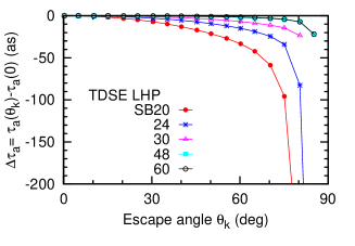
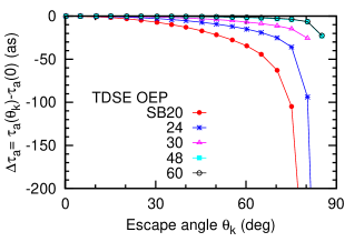
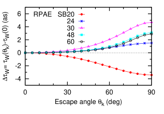
Figure 4: (Color online) Angular variation of the atomic time delay $\Delta\tau_{a}=\tau_{a}(\theta_{k})-\tau_{a}(0)$ in various sidebands of the Ne $2p$ RABBITT trace calculated with the LHF potential (top) and the OEP potential (middle). Bottom: angular variation of the Wigner time delay $\Delta\tau_{\rm W}=\tau_{\rm W}(\theta_{k})-\tau_{\rm W}(0)$ from the XUV-only RPAE calculation.

Angular dependence of the atomic time delay $\tau_{a}(\theta_{k})$ as a function of the escape angle is shown in Fig. 4. The top and middle panels display the TDSE calculations with the LHF and OEP potentials, respectively. The bottom panel shows the angular dependence of the Wigner time delay $\tau_{\rm W}(\theta_{k})$ from the XUV-only RPAE calculation. We see that both TDSE calculations are quite close to one another while the RPAE calculation suggests an angular dependence which is an order of magnitude weaker. The consequence being that nearly all the angular dependence of the atomic time delay in Ne comes from the CC correction introduced by the probe IR field. A similar observation was made in He where the Wigner time delay is isotropic Heuser et al. (2016). In Ne, the Wigner time delay is not entirely isotropic because the $2p\to\epsilon s$ and $2p\to\epsilon d$ channels enter the ionization amplitude with their own spherical harmonics, namely $Y_{00}(\theta_{k})$ and $Y_{20}(\theta_{k})$. However, as a result of the Fano propensity rule Fano (1985), the $d$-continuum is strongly dominant and the $s$-continuum contributes only a very weak angular modulation. We note that this situation would change drastically near the CM in Ar and heavier noble gases where the angular dependence of the Wigner time delay is very strong.

The time delay in the polarization axis direction $\theta_{k}=0$ is shown in Fig. 5. On the top panel, we compare the atomic time delay from the TDSE calculation with the LHF potential and the Wigner time delay $\tau_{\rm W}$ from the RPAE calculation. The hydrogenic CC correction $\tau_{\rm CC}$, which is shown separately, is then added to the Wigner time delay. This correction, as a function of the photoelectron energy, is represented by the analytic expression

$$\tau_{\rm CC}(E)=NE^{-3/2}[a\log(E)+b]$$ (18)

where the coefficients $N$, $a$ and $b$ are found from fitting the regularized continuum-continuum delay shown in Fig. 7 of Dahlström et al. (2012b). We see that except for the near threshold region where the photoelectron energy is very small and where the regularization of $\tau_{\rm CC}$ may not be applicable, the identity (1) $\tau_{a}\simeq\tau_{W}+\tau_{cc}$ holds very well.

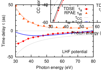
Figure 5: (Color online) Time delay in the polarization axis direction $\theta_{k}=0$. Top: the atomic time delay $\tau_{a}$ from the TDSE calculation (red filled circles) is compared with the Wigner time delay (orange triangle) from the RPAE calculation. The CC correction $\tau_{\rm CC}$ is shown with the thin dotted line whereas the sum $\tau_{\rm W}+\tau_{\rm CC}$ is displayed with the (blue) dotted line. Bottom: the CC correction $\tau_{\rm CC}$ (thin dotted line) is compared with the atomic and Wigner time delay difference $\tau_{a}-\tau_{\rm W}$ from the TDSE calcualtions with the LHF and OEP potentials (shown with the red filled and black open circles).

This utility of the hydrogenic CC correction can be used to analyze the recent set of RABBITT measurements on Ne Isinger et al. (2017) where the time delay difference between the $2s$ and $2p$ shells in Ne was determined. This analysis is shown in Fig. 6. On the top panel, we plot the Wigner time delay from the RPAE calculation for the individual $2s$ and $2p$ shells and their difference. On the bottom panel, the Wigner time delay difference is augmented by that of the CC correction. We assume that the CC correction $\tau_{\rm CC}$ is a universal function of the photoelectron energy and as such the CC correction difference between shells at the same photon energy is caused by their varying ionization potentials. The atomic time delay difference

$$\tau_{a}(2s)-\tau_{a}(2p) = \tau_{\rm W}(2s)-\tau_{\rm W}(2p)$$

$$+ \tau_{\rm CC}(2s)-\tau_{\rm CC}(2p)$$

is compared with the RABBITT measurement and the RPA calculation presented in Isinger et al. (2017). We see that both calculations (almost indistinguishable in the scale of the figure) reproduce the measurement Isinger et al. (2017) very well. In contrast, the older measurement Schultze et al (2010) deviates from the theoretical predictions by nearly a factor of 2.

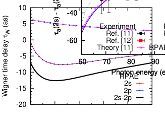
Figure 6: (Color online) Top: the Wigner time delay in the $2s$ and $2p$ shells of Ne and their difference. Bottom: the atomic time delay difference $\tau_{a}(2s)-\tau_{a}(2p)$ as measured experimentally by Isinger et al. (2017) (filled circles) and Schultze et al (2010) (red square). The Wigner time delay difference $\tau_{\rm W}(2s)-\tau_{\rm W}(2p)$ (red solid line) is augmented by the CC correction difference $\tau_{\rm CC}(2s)-\tau_{\rm CC}(2p)$ (dotted line) to get the atomic time delay difference $\tau_{a}(2s)-\tau_{a}(2p)$ (blue solid line) which is compared with the calculated result of Isinger et al. (2017) (purple dashed line).

III.2 Argon $3p$ shell

The $\beta$ parameters for the Ar $3p$ shell extracted from the angular dependence of the high harmonic peaks and sidebands are shown in Fig. 7. The TDSE calculations performed with the LHF and OEP potentials are shown on the top and bottom panels, respectively. The three sets of $\beta$ parameters are compared with the RPAE calculation and the experiment Houlgate et al. (1974). We observe from this figure that all three sets of $\beta$ parameters extracted from the TDSE calculation with the LHF potential follow closely the RPAE prediction and agree with the experiment. At the same time, the OEP TDSE results are displaced relative to the RPAE in the photon energy scale by as much as 10 eV. This mismatch is a reflection of the displacement of the CM position in the photoionization cross-section. This position can be located very accurately from the squared radial integral Mauritsson et al. (2005)

$$\left|\int\limits_{0}^{\infty}P_{3p}(r)P_{Ed}(r)\ rdr\right|^{2}\ .$$ (20)

A plot of this integral is given in Fig. 8 where the radial orbitals of the bound and continuous states have been calculated from the Schrödinger equation with Hamiltonian (3) using the LHF, OEP, Muller Muller (2002b) and Miller and Dow (1977) potentials. The equivalent value from the HF and RPAE calculations are also shown. We see that the CM position is misplaced for each of the potentials except the LHF. Subsequently, in the following, we present our TDSE results calculated with the LHF potential only.

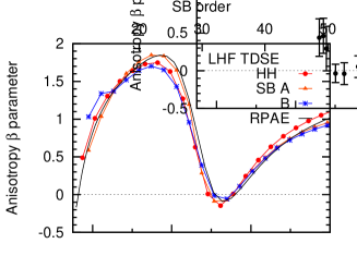
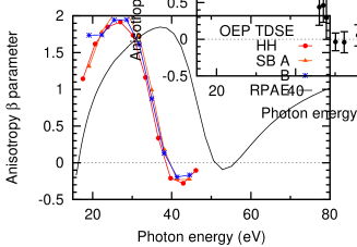
Figure 7: (Color online) Same as Fig. 3 for Ar $3p$ shell. The experiment Houlgate et al. (1974) is given by the points with error bars.

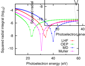
Figure 8: (Color online) The squared radial integral (20) calculated with the LHF (red filled circles), OEP (open green circles), Miller and Dow (1977) (blue asterisks) and Muller Muller (2002b) (purple triangles) potentials for Ar. The HF and RPAE results are shown with black dotted and solid lines respectively.

In Fig. 9 we compare $\beta_{2}$ and $\beta_{4}$ parameters as measured by Cirelli et al. (2018) and those expressed in Eq. (11). On the top panel we compare $\beta_{2}$ and $\beta^{\rm HH}$ derived from the main harmonic peaks while on the bottom panel we display $\beta_{2},\beta_{4}$ as measured directly from the SB amplitude and as expressed via $\beta^{\rm SB}(A)$ and $\beta^{\rm SB}(B)$ in Eq. (11). We see that the $\beta_{4}$ parameters compare rather favourably whereas the $\beta_{2}$ parameters are a bit higher than in the experiment.

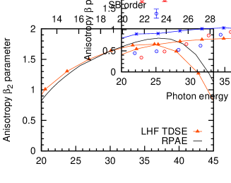
Figure 9: (Color online) Top: the anisotropy parameters derived from the angular variation of the high harmonic peaks. The two sets of experimental values $\beta_{2}$ from Cirelli et al. (2018) are shown by open circles with error bars. The synchrotron measurement Southworth et al. (1986) is shown with black dots. The orange triangles connected with solid line visualize $\beta^{\rm HH}$ from the LHF TDSE calculation whereas the black solid line displays the RPAE result. Bottom: the experimental $\beta_{2}$ and $\beta_{4}$ parameters are shown by the same symbols as on the top panel. The same parameters extracted from the LHF TDSE calculation are shown with purple triangles (derived from $A$ parameter) and blue asterisks ($B$ parameter).

The angular variations of the atomic time delay $\Delta\tau_{a}=\tau_{a}(\theta_{k})-\tau_{a}(0)$ in various sidebands of the Ar $3p$ RABBITT trace, and the Wigner time delay angular variation $\Delta\tau_{\rm W}=\tau_{\rm W}(\theta_{k})-\tau_{\rm W}(0)$ at the same photon energies, are displayed in Fig. 10 (top and bottom panels respectively). In stark contrast to the analogous set of data for Ne $2p$ shown in Fig. 4, the angular variation of the Wigner time delay for Ar $3p$ is of the same order of magnitude, and is almost identical for SB30 near the CM. As a reference, in both panels of Fig. 10, the LOPT calculation Dahlström and Lindroth (2014) for SB32 is shown. Beyond the CM (SB48 and SB60), the angular variation of the Wigner time delay flattens whereas the same variation of the atomic time delay changes its sign and simultaneously lessens in magnitude.

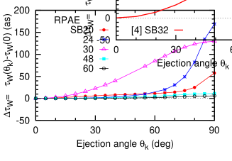
Figure 10: (Color online) Top: angular variation of the atomic time delay $\Delta\tau_{a}=\tau_{a}(\theta_{k})-\tau_{a}(0)$ in various sidebands of the Ar $3p$ RABBITT trace calculated with the LHF potential. Bottom: angular variation of the Wigner time delay $\Delta\tau_{\rm W}=\tau_{\rm W}(\theta_{k})-\tau_{\rm W}(0)$ from the XUV-only RPAE calculation. The angular variation of time delay for SB32 from Dahlström and Lindroth (2014) is shown for comparison.

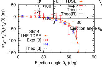
Figure 11: (Color online) Same as Fig. 10 for SB14 (top) and SB16 (bottom). Two sets of measurements from Cirelli et al. (2018) are shown by open circles with error bars. The LOPT result from the same work is visualized by a dashed line. The LHF TDSE result is shown with orange triangles connected by the solid line. The bottom panel also shows the calculation from Cirelli et al. (2018) which includes the Fano resonance (black solid line).

In Fig. 11 we compare the angular variation of the atomic time delay $\Delta\tau_{a}=\tau_{a}(\theta_{k})-\tau_{a}(0)$ in SB14 (top) and SB16. In the experiment Cirelli et al. (2018), SB16 is tuned in resonance with the $4s^{-1}5p$ autoionizing state while SB14 is off the resonance. For SB14 we find a fairly good agreement between the experiment and the present LHF TDSE calculation. The LOPT calculation reported in Cirelli et al. (2018) is also very close. For SB16 both the TDSE and LOPT calculations predict considerably weaker angular dependence than in the experiment and the calculation which accounts for resonance by the Fano configuration interaction formalism.

Various time delays for the Ar $3p$ shell in the zero angle polarization direction are shown in Fig. 12. On the top panel, we display the atomic time delay $\tau_{a}$ from the TDSE LHF calculation, the Wigner time delay $\tau_{\rm W}$ from the RPAE calculation, the regularized hydrogenic CC correction $\tau_{\rm CC}$ and their sum $\tau_{\rm W}+\tau_{\rm CC}$. We also show the atomic time delay $\tau_{a}$ from the LOPT calculation Dahlström and Lindroth (2014). The latter is almost indistinguishable from the sum $\tau_{\rm W}+\tau_{\rm CC}$, but visibly different from the TDSE calculation for $\tau_{a}$. On the bottom panel we show the hydrogenic $\tau_{\rm CC}$ and the argon specific value $\tau_{\rm CC}=(\phi^{-}_{\rm CC}-\phi^{+}_{\rm CC})/2\omega$ obtained from the phases $\phi^{\pm}_{\rm CC}$ reported in Cirelli et al. (2018). Both values, which are remarkably close, are compared with the difference $\tau_{a}-\tau_{\rm W}$. Unlike in the Ne $2p$ case, displayed on the bottom panel of Fig. 5, these two derivations of the CC correction give quite different results. This difference may, in principle, be attributed to the different approximations used in TDSE-LHF and RPAE calculations. The former employes a localized version of the HF potential and neglects the correlation while the latter gives the full account to the exchange and inter-shell correlation. However, the same calculations return quite similar sets of $\beta$ parameters. As such it is more likely that the hydrogenic approximation to $\tau_{\rm CC}$ breaks for the argon $3p$ shell.

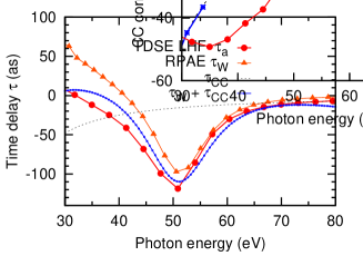
Figure 12: (Color online) Same as Fig. 5 for Ar $3p$ shell. In addition, the atomic time delay $\tau_{a}$ from the LOPT calculation Dahlström and Lindroth (2014) and the CC correction $\tau_{\rm CC}=(\phi^{-}_{\rm CC}-\phi^{+}_{\rm CC})/2\omega$ obtained from the phases $\phi^{\pm}_{\rm CC}$ reported in Cirelli et al. (2018) are shown.

This break down may have implications to theoretical interpretation of the time delay difference in the valence shell of Ar shown in Fig. 13. Here the atomic time delay difference

$$\tau_{a}(3s)-\tau_{a}(3p) = \tau_{\rm W}(3s)-\tau_{\rm W}(3p)$$

$$+ \tau_{\rm CC}(3s)-\tau_{\rm CC}(3p)$$

is computed with the hydrogenic CC corrections and compared with the RABBITT measurement Guénot et al. (2012). As $\tau_{\rm CC}(3p)$ deduced from the present TDSE calculation is more negative by about 20 as near the 40 eV mark as compared to the hydrogenic estimate, the atomic time delay difference estimated from Eq. (III.2) will be shifted upwards by the same amount. It will make the disagreement with the measurement Guénot et al. (2012) even worse. The present TDSE calculation is not able to give an estimate to $\tau_{\rm CC}(3s)$ as ionization of this shell is strongly correlated with that of the valence $3p$ shell and goes beyond the SAE approximation.

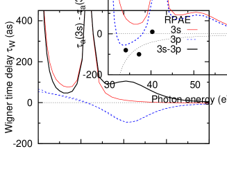
Figure 13: (Color online) Top: the Wigner time delay in the $3s$ and $3p$ shells of Ar and their difference. Bottom: the atomic time delay difference $\tau_{a}(3s)-\tau_{a}(3p)$ as measured experimentally by Guénot et al. (2012) (filled circles). The Wigner time delay difference $\tau_{\rm W}(3s)-\tau_{\rm W}(3p)$ (red solid line) is augmented by the CC correction difference $\tau_{\rm CC}(3s)-\tau_{\rm CC}(3p)$ (dotted line) to get the atomic time delay difference $\tau_{a}(3s)-\tau_{a}(3p)$ (blue dashed line).

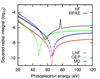
Figure 14: (Color online) The squared radial integral (20) calculated with the LHF (red filled circles), OEP (open green circles), Muller Muller (2002b) (blue asterisks) and Miller&Dow Miller and Dow (1977) (purple triangles) potentials for Kr. The HF and RPAE results are shown with black dotted and solid lines respectively.

III.3 Krypton $4p$ shell

We test validity of various effective potentials for Kr by determining the CM position in the $4p$ photoionization cross-section. We do so by comparing the squared radial integrals (20) calculated with the bound state $4p$ orbital and the continuous $d$-wave obtained from the radial Schrödinger equation Eq. (3). This comparison is shown in Fig. 14. Unlike in the case of Ar $3p$ photoionization, illustrated in Fig. 8, the CM position calculated in the HF and RPAE differs by nearly 20 eV. This is so because of the influence of the inter-shell correlation between the $4p$ and $3d$ shells and which is accounted for in the RPAE but not in the HF calculation. This correlation is absent in the case of Ar $3p$ as the $3d$ shell is vacant for this atom. The CM position calculated with the LHF and MD potentials is in between the HF and RPAE whereas the OEP calculation displaces the CM to lower energies very significantly. We discard the OEP in the following.

The three sets of angular anisotropy $\beta$ parameters extracted from the high harmonic peaks and the side bands are shown in Fig. 15 calculated with the LHF (top) and MD (bottom) potentials. We see that agreement between the TDSE and RPAE calculations is generally good but these calculations diverge at higher photon energies. This occurs well below the $3d$ threshold whose position can be identified by the converging autoionization resonances visible in the RPAE curve. The experiment Miller et al. (1977) clearly favors the RPAE calculation. Partial agreement between the TDSE calculations with the LHF and MD potentials, the RPAE and the experiment may be somewhat fortuitous given a strong deviation of the TDSE binding energies from the experimental threshold (see Table 1). Should the $\beta$ parameters in Fig. 15 be plotted versus the photoelectron energy, this agreement will disappear.

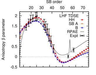
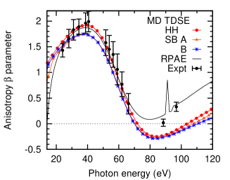
Figure 15: (Color online) Same as Fig. 3 for the Kr $4p$ shell. The experimental data are from Miller et al. (1977).

III.4 Xenon $5p$ shell

This tendency of deviation of the TDSE calculations with various local potentials from the RPAE and experiment is aggravated further in Xe. As an illustration, we show in Fig. 16 the CM position deduced from the squared radial integral (20). Firstly, we observe that the HF and RPAE results diverge by as much as 40 eV. This is a clear sign of a very strong correlation between the $5p$ and $4d$ shells accounted for in the RPAE but missing in the HF. Second, both the LHF and OEP give the CM position which is displaced by 20 eV from the RPAE for the same reason.

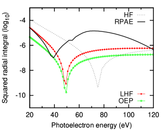
Figure 16: (Color online) The squared radial integral (20) calculated with the LHF (red filled circles), and OEP (open green circles) potentials for Xe. The HF and RPAE results are given by the black dotted and solid lines respectively.

It is well known that missing the inter-shell correlation between the $5p$ and $4d$ shells in Xe has a profound effect on the anisotropy $\beta$ parameter. It becomes strongly displaced relative to the experiment as shown graphically in Fig. 1 of West (1980). We therefore do not expect any reasonable agreement of the presently employed TDSE/SAE model with the experiment either.

IV Conclusions

We presented a series of simulations and their analysis for the angular dependent RABBITT traces in the valence shells of noble gas atoms from Ne to Xe. Our simulations are based on numerical solutions of the one-electron TDSE driven with the XUV ionizing field and the IR probing pulse. Exchange between the departing photoelectron and the ionized atomic core is accounted for by various effective one-electron potentials. The accuracy of this account is tested by making comparison with the Hartree-Fock approximation which includes the exchange by constriction. The inter-shell correlation between the valence $np$ and sub-valent $ns,(n-1)d$ shells are neglected in a one-electron TDSE. To elucidate the strength of this correlation, we compare the TDSE results with the RPAE calculation which is known to account for the inter-shell correlation very accurately. However, the RPAE is unable to account for ultrafast electron dynamics and designed for much slower ionization processes initiated by long pulses of synchrotron radiation.

We focus our analysis on the anisotropy $\beta$ parameter which is extracted from the angular dependence of the high harmonic peaks as well as sideband RABBITT oscillation amplitude $A$ and $B$ factors. Within the scope of the soft photon approximation, all the three sets of $\beta$ should be in agreement which was found to be the case. This streamlines considerably the analysis of a angular resolved RABBITT measurement and makes redundant the introduction of multiple sets of angular anisotropy parameters which was made by Cirelli et al. (2018). The phase of the RABBITT oscillation is converted to the angular dependent time delay which is compared with the RPAE calculations. The time delay in the polarization direction is used to test accuracy of the hydrogenic CC correction.

Our results can be broadly categorized into the two groups. In lighter atoms, Ne and Ar, the single active electron model is generally valid. The Ne calculations are particularly robust with all the tested effective potentials producing accurate results close to the RPAE predictions both for the angular anisotropy and the time delay. In Ar, because of the appearance of the Cooper minimum, the TDSE calculations become very sensitive to the choice of the effective potential and a simple analytic fit to the localized HF potential produces the best results for $\beta$ parameters. At the same time, this calculation suggests deviation of the CC correction from the regularized hydrogenic expression. Because of the Cooper minimum, the angular variation of the Wigner time delay is of the same magnitude as the that variation of the atomic time delay. In Ne, the angular variation of the Wigner time delay is negligible.

In heavier atoms, in Kr and particularly in Xe, the inter-shell correlation between the valence $np$-shell and sub-valent $(n-1)d$ shell becomes very strong. In Kr, with some choice of effective potentials, the present model can return sensible Cooper minimum position and $\beta$ parameters away from the $(n-1)d$ shell threshold. In Xe, no effective potential is expected to replace the strong effect of inter-shell correlation and the present model is generally invalid.

Our findings are of importance to the theoretical analysis of angular resolved RABBITT measurements. Particularly that there is a linear dependence of the $\beta_{2}$ and $\beta_{4}$ parameters which can be derived from the single set describing the whole RABBITT measurement, both the high harmonic peaks and the side bands. This set can be easily compared with predictions of the RPAE theory which is valid for all noble gas atoms. These $\beta$ parameters can also be tested against the XUV only measurements Codling et al. (1976); Houlgate et al. (1974); Miller et al. (1977); West (1980); Southworth et al. (1986).

This work is a step forward in resolving the persistent controversy in the time delay measurement in Ar Guénot et al. (2012). However, as the measurement involved both the valence $3p$ and the sub-valent $3s$ shells, we are unable to conclusively do so. The $3s$ shell in argon is strongly correlated with the $3p$ shell and this inter-shell correlation goes beyond the scope of the present model.

The model, as it stands now, can be applied to the sub-valent Kr $3d$ and Xe $4d$ shells which are not effected strongly by inter-shell correlation with outer valence shells. The $nd$ correlation with inner core is only noticeable near corresponding deeper thresholds. We can also easily incorporate the effect of a fullerene cage Mandal et al. (2017) to model a RABBITT process in encapsulated atoms. Eventually, we will attempt to generalize our model to account for inter-shell correlation. This will require considerable development of the existing one-electron TDSE code.

Appendix: RABBITT in soft photon approximation

We start from Eqs. (10) and (11) of Maquet and Taïeb (2007) and write the amplitude of the XUV photon absorption modulated by absorption ($+$) or emission ($-$) of $n$ IR photons as

$$S\phantom{{}_{n}} = \sum_{n=-\infty}^{+\infty}S_{n}\delta(k^{2}/2-E_{0}-\omega_{x}-n\omega)$$ (A1 )

$$S_{n} = -2\pi iJ_{-n}({\bm{a}}_{0}\cdot{\bm{k}}_{n})\exp[-i(\phi_{x}+n\phi)]\langle{\bm{k}}_{n}|{\bm{\epsilon}}\cdot\nabla|i\rangle$$

with $k_{n}\simeq[2(E_{0}+\omega_{x}+n\omega)]^{1/2}$ being the shifted momentum of the photoelectron and $\omega_{x}$, $\phi_{x}$ and $\omega$, $\phi$ as the XUV and IR frequencies and phase shifts respectively. Here the matrix element $\langle{\bm{k}}_{n}|{\bm{\epsilon}}\cdot\nabla|i\rangle$ of the XUV photon absorption is written in the velocity gauge.

In RABBITT we are only interested in the $n=1$ and $n=-1$ sidebands. Their corresponding amplitudes are

$$S_{\pm 1}\equiv{\cal M}^{(\pm)}_{{\bm{k}}_{\pm 1}} = -2\pi iJ_{\mp 1}({\bm{a}}_{0}\cdot{\bm{k}}_{\pm 1})$$

$$\times \exp[\mp i\phi^{\pm}_{\rm CC}]\langle{{\bm{k}}_{\pm 1}}|{\bm{\epsilon}}\cdot\nabla|i\rangle\ .$$

Here we introduced the phase $\phi^{\pm}_{\rm CC}$ associated with the continuum-continuum transition in absorption or emission of an IR photon. For simplicity we have dropped the XUV phase $\phi_{x}$ and thus neglected the harmonic group delay. Using the transformation $J_{-n}=(-1)^{n}J_{n}$ we write

$$S_{+1}+S_{-1} =$$

$$-2\pi i\Big{[}J_{1}({\bm{a}}_{0}\cdot{\bm{k}}_{-1})\langle{{\bm{k}}_{-1}}|{\bm{\epsilon}}\cdot\nabla|i\rangle\ e^{\displaystyle-i\phi^{+}_{\rm CC}}$$

$$-J_{1}({\bm{a}}_{0}\cdot{\bm{k}}_{+1})\langle{{\bm{k}}_{+1}}|{\bm{\epsilon}}\cdot\nabla|i\rangle\ e^{\displaystyle+i\phi^{-}_{\rm CC}}\Big{]}\ .$$

We can relate the phases of the dipole matrix elements with the soft photon shifted momenta by the phase energy derivative,

$$\langle{{\bm{k}}_{\pm 1}}|{\bm{\epsilon}}\cdot\nabla|i\rangle \approx \langle{\bm{k}}|{\bm{\epsilon}}\cdot\nabla|i\rangle e^{\pm i\omega\partial\delta_{m_{i}}({\bm{k}})/\partial E}$$

$$\delta_{m_{i}}({\bm{k}}) = \arg\langle{\bm{k}}|{\bm{\epsilon}}\cdot\nabla|i\rangle\ .$$ (A4 )

Further, we assume $J_{1}({\bm{\alpha}}_{0}\cdot{\bm{k}}_{\pm 1})\approx J_{1}({\bm{\alpha}}_{0}\cdot{\bm{k}})$ and subsequently find the magnitude of the RABBITT signal (8) to be proportional to

$${\rm Re}\left[{\cal M}^{(-)}_{{\bm{k}}}{\cal M}^{*(+)}_{{\bm{k}}}\right] \propto \big{|}J_{1}({\bm{\alpha}}_{0}\cdot{\bm{k}})\big{|}^{2}\Big{[}\sum_{m_{i}}|\langle\chi_{\bm{k}}|{\bm{\epsilon}}\cdot\nabla|\psi_{i}\rangle|^{2}\Big{]}$$ (A5 )

$$\propto \cos^{2}\theta\Big{[}1+\beta P_{2}(\cos\theta)\Big{]}\ .$$

Here we used the expansion $J_{1}(x)\simeq x/2+O(x^{3})$ valid for a weak IR field and accordingly small parameter ${\bm{\alpha}}_{0}={\bm{F}}_{0}/\omega^{2}\ .$ We also performed the angular momentum projection summation Amusia (1990)

$$\sum_{m_{i}}|\langle{\bm{k}}|{\bm{\epsilon}}\cdot\nabla|i\rangle|^{2}\propto{\sigma_{i}\over 4\pi}\Big{[}1+\beta P_{2}(\cos\theta)\Big{]}\ ,$$ (A6 )

where $\beta$ is the angular anisotropy parameter and $\sigma_{i}$ is the photoionization cross-section of the $i$-th atomic shell.

The atomic time delay is given by

$$\tau = {1\over 2\omega}\arg\left[{\cal M}^{(-)}_{{\bm{k}}}{\cal M}^{*(+)}_{{\bm{k}}}\right]$$

$$\equiv {1\over 2\omega}\arg\Big{[}\sum_{m_{i}}|c_{m_{i}}|^{2}e^{2i\phi_{m_{i}}}\Big{]}+{\phi^{-}_{\rm CC}-\phi^{+}_{\rm CC}\over 2\omega}$$

$$\equiv \tau_{\rm W}+\tau_{\rm CC}$$

where we have used the shorthand

$$\phi_{m_{i}}=\omega\ {\partial\delta_{m_{i}}({\bm{k}})\over\partial E}\ ,\ c_{m_{i}}=\langle\chi_{\bm{k}}|{\bm{\epsilon}}\cdot\nabla|\psi_{i}\rangle$$

for the quantities associated with the XUV photon absorption which define the Wigner time delay $\tau_{\rm W}$.

References

- Laurent et al. (2012) G. Laurent, W. Cao, H. Li, Z. Wang, I. Ben-Itzhak, and C. L. Cocke, Attosecond control of orbital parity mix interferences and the relative phase of even and odd harmonics in an attosecond pulse train, Phys. Rev. Lett. 109, 083001 (2012).
- Heuser et al. (2016) S. Heuser, A. Jiménez Galán, C. Cirelli, C. Marante, M. Sabbar, R. Boge, M. Lucchini, L. Gallmann, I. Ivanov, A. S. Kheifets, et al., Angular dependence of photoemission time delay in helium, Phys. Rev. A 94, 063409 (2016).
- Cirelli et al. (2018) C. Cirelli, C. Marante, S. Heuser, C. L. M. Petersson, A. J. Galán, L. Argenti, S. Zhong, D. Busto, M. Isinger, S. Nandi, et al., Anisotropic photoemission time delays close to a Fano resonance, Nature Comm. 9, 955 (2018).
- Dahlström and Lindroth (2014) J. M. Dahlström and E. Lindroth, Study of attosecond delays using perturbation diagrams and exterior complex scaling, J. Phys. B 47(12), 124012 (2014).
- Hockett (2017) P. Hockett, Angle-resolved RABBITT: theory and numerics, J. Phys. B 50(15), 154002 (2017).
- Ivanov and Kheifets (2017) I. A. Ivanov and A. S. Kheifets, Angle-dependent time delay in two-color XUV+IR photoemission of He and Ne, Phys. Rev. A 96, 013408 (2017).
- Muller (2002a) H. Muller, Reconstruction of attosecond harmonic beating by interference of two-photon transitions, Appl. Phys. B 74, s17 (2002a).
- Toma and Muller (2002) E. S. Toma and H. G. Muller, Calculation of matrix elements for mixed extreme-ultraviolet–infrared two-photon above-threshold ionization of argon, J. Phys. B 35(16), 3435 (2002).
- Sarsa et al. (2004) A. Sarsa, F. J. Gálvez, and E. Buendia, Parameterized optimized effective potential for the ground state of the atoms He through Xe, Atomic Data and Nuclear Data Tables 88(1), 163 (2004).
- Guénot et al. (2012) D. Guénot, K. Klünder, C. L. Arnold, D. Kroon, J. M. Dahlström, M. Miranda, T. Fordell, M. Gisselbrecht, P. Johnsson, J. Mauritsson, et al., Photoemission-time-delay measurements and calculations close to the 3-ionization-cross-section minimum in Ar, Phys. Rev. A 85, 053424 (2012).
- Isinger et al. (2017) M. Isinger, R. Squibb, D. Busto, S. Zhong, A. Harth, D. Kroon, S. Nandi, C. L. Arnold, M. Miranda, J. M. Dahlström, et al., Photoionization in the time and frequency domain, Science (2017).
- Schultze et al (2010) M. Schultze et al, Delay in Photoemission, Science 328(5986), 1658 (2010).
- Kheifets and Ivanov (2010) A. S. Kheifets and I. A. Ivanov, Delay in atomic photoionization, Phys. Rev. Lett. 105(23), 233002 (2010).
- Moore et al. (2011) L. R. Moore, M. A. Lysaght, J. S. Parker, H. W. van der Hart, and K. T. Taylor, Time delay between photoemission from the and subshells of neon, Phys. Rev. A 84, 061404 (2011).
- Dahlström et al. (2012a) J. M. Dahlström, T. Carette, and E. Lindroth, Diagrammatic approach to attosecond delays in photoionization, Phys. Rev. A 86, 061402 (2012a).
- Kheifets (2013) A. S. Kheifets, Time delay in valence-shell photoionization of noble-gas atoms, Phys. Rev. A 87, 063404 (2013).
- Feist et al. (2014) J. Feist, O. Zatsarinny, S. Nagele, R. Pazourek, J. Burgdörfer, X. Guan, K. Bartschat, and B. I. Schneider, Time delays for attosecond streaking in photoionization of neon, Phys. Rev. A 89, 033417 (2014).
- Omiste and Madsen (2018) J. J. Omiste and L. B. Madsen, Attosecond photoionization dynamics in neon, Phys. Rev. A 97, 013422 (2018).
- Morales et al. (2016) F. Morales, T. Bredtmann, and S. Patchkovskii, isurf: a family of infinite-time surface flux methods, J. Phys. B 49(24), 245001 (2016).
- Maquet and Taïeb (2007) A. Maquet and R. Taïeb, Two-colour ir+xuv spectroscopies: the soft-photon approximation, J. Modern Optics 54(13-15), 1847 (2007).
- Kheifets et al (2016) A. S. Kheifets et al, Relativistic calculations of angle-dependent photoemission time delay, Phys. Rev. A 94, 013423 (2016).
- Dahlström et al. (2012b) J. Dahlström, D. Guénot, K. Klünder, M. Gisselbrecht, J. Mauritsson, A. L. Huillier, A. Maquet, and R. Taïeb, Theory of attosecond delays in laser-assisted photoionization, Chem. Phys. 414, 53 (2012b).
- Slater (1951) J. C. Slater, A simplification of the Hartree-Fock method, Phys. Rev. 81, 385 (1951).
- Miller and Dow (1977) D. L. Miller and J. D. Dow, Atomic pseudopotentials for soft x-ray excitations, Physics Letters A 60(1), 16 (1977).
- Muller (2002b) H. Muller, Reconstruction of attosecond harmonic beating by interference of two-photon transitions, Applied Physics B 74(1), s17 (2002b).
- Jones and Gunnarsson (1989) R. O. Jones and O. Gunnarsson, The density functional formalism, its applications and prospects, Rev. Mod. Phys. 61, 689 (1989).
- Wendin and Starace (1978) G. Wendin and A. F. Starace, Perturbation theory in a strong-interaction regime with application to 4d-subshell spectra of ba and la, J. Phys. B 11(24), 4119 (1978).
- Ralchenko et al. (2011) Y. Ralchenko, A. E. Kramida, J. Reader, and NIST ASD Team, NIST atomic spectra database (version 3.1.5) (2011), URL http://physics.nist.gov/asd.
- Codling et al. (1976) K. Codling, R. G. Houlgate, J. B. West, and P. R. Woodruff, Angular distribution and photoionization measurements on the 2p and 2s electrons in neon, J. Phys. B 9(5), L83 (1976).
- Fano (1985) U. Fano, Propensity rules: An analytical approach, Phys. Rev. A 32, 617 (1985).
- Houlgate et al. (1974) R. G. Houlgate, K. Codling, G. V. Marr, and J. B. West, Angular distribution and photoionization cross section measurements on the 3p and 3s subshells of argon, J. Phys. B 7(17), L470 (1974).
- Mauritsson et al. (2005) J. Mauritsson, M. B. Gaarde, and K. J. Schafer, Accessing properties of electron wave packets generated by attosecond pulse trains through time-dependent calculations, Phys. Rev. A 72, 013401 (2005).
- Southworth et al. (1986) S. Southworth, A. Parr, J. Hardis, J. Dehmer, and D. Holland, Calibration of a monochromator/spectrometer system for the measurement of photoelectron angular distributions and branching ratios, Nucl. Instr. Methods A 246(1), 782 (1986).
- Miller et al. (1977) D. L. Miller, J. D. Dow, R. G. Houlgate, G. V. Marr, and J. B. West, The photoionisation of krypton atoms: a comparison of pseudopotential calculations with experimental data for the 4p asymmetry parameter and cross section as a function of the energy of the ejected photoelectrons, J. Phys. B 10(16), 3205 (1977).
- West (1980) J. B. West, Progress in photoionization spectroscopy of atoms and molecules: an experimental viewpoint, Appl. Opt. 19(23), 4063 (1980).
- Mandal et al. (2017) A. Mandal, P. C. Deshmukh, A. S. Kheifets, V. K. Dolmatov, and S. T. Manson, Angle-resolved wigner time delay in atomic photoionization: The subshell of free and confined Xe, Phys. Rev. A 96, 053407 (2017).
- Amusia (1990) M. Y. Amusia, Atomic photoeffect (Plenum Press, New York, 1990).