Constant-Time Predictive Distributions for Gaussian Processes

Abstract

One of the most compelling features of Gaussian process (GP) regression is its ability to provide well-calibrated posterior distributions. Recent advances in inducing point methods have sped up GP marginal likelihood and posterior mean computations, leaving posterior covariance estimation and sampling as the remaining computational bottlenecks. In this paper we address these shortcomings by using the Lanczos algorithm to rapidly approximate the predictive covariance matrix. Our approach, which we refer to as LOVE (LanczOs Variance Estimates), substantially improves time and space complexity. In our experiments, LOVE computes covariances up to $2,\!000$ times faster and draws samples $18,\!000$ times faster than existing methods, all without sacrificing accuracy.

1 Introduction

Gaussian processes (GPs) are fully probabilistic models which can naturally estimate predictive uncertainty through posterior variances. These uncertainties play a pivotal role in many application domains. For example, uncertainty information is crucial when incorrect predictions could have catastrophic consequences, such as in medicine (Schulam & Saria, 2017) or large-scale robotics (Deisenroth et al., 2015); Bayesian optimization approaches typically incorporate model uncertainty when choosing actions (Snoek et al., 2012; Deisenroth & Rasmussen, 2011; Wang & Jegelka, 2017); and reliable uncertainty estimates are arguably useful for establishing trust in predictive models, especially when predictions would be otherwise difficult to interpret (Doshi-Velez & Kim, 2017; Zhou et al., 2017).

Although predictive uncertainties are a primary advantage of GP models, they have recently become their computational bottleneck. Historically, the use of GPs has been limited to problems with small datasets, since learning and inference computations naïvely scale cubically with the number of data points ($n$). Recent advances in inducing point methods have managed to scale up GP training and computing predictive means to larger datasets (Snelson & Ghahramani, 2006; Quiñonero-Candela & Rasmussen, 2005; Titsias, 2009). Kernel Interpolation for Scalable Structured GPs (KISS-GP) is one such method that scales to millions of data points (Wilson & Nickisch, 2015; Wilson et al., 2015). For a test point $\mathbf{x}^{*}$, KISS-GP expresses the predictive mean as ${{\color[rgb]{0,0,1}\mathbf{a}}^{\top}}\mathbf{w}(\mathbf{x}^{*})$, where ${\color[rgb]{0,0,1}\mathbf{a}}$ is a pre-computed vector dependent only on training data, and $\mathbf{w}(\mathbf{x}^{*})$ is a sparse interpolation vector. This formulation affords the ability to compute predictive means in constant time, independent of $n$.

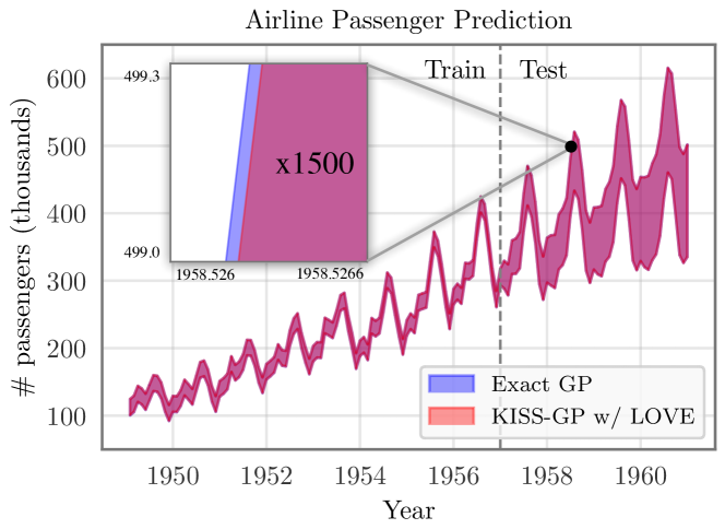
Figure 1: Comparison of predictive variances on airline passenger extrapolation. The variances predicted with LOVE are accurate within $10^{-4}$, yet can be computed orders of magnitude faster.

However, these computational savings do not extend naturally to predictive uncertainties. With KISS-GP, computing the predictive covariance between two points requires $\mathcal{O}(n+m\log m)$ computations, where $m$ is the number of inducing points (see Table 1). While this asymptotic complexity is lower than standard GP inference and alternative scalable approaches, it becomes prohibitive when $n$ is large, or when making many repeated computations. Additionally, drawing samples from the predictive distributions – a necessary operation in many applications – is similarly expensive. Existing fast approximations for these operations (Papandreou & Yuille, 2011; Wilson et al., 2015; Wang & Jegelka, 2017) typically incur a significant amount of error. Matching the reduced complexity of predictive mean inference without sacrificing accuracy has remained an open problem.

Table 1: Asymptotic complexities of predictive (co)variances ($n$ training points, $m$ inducing points, $k$ Lanczos/CG iterations) and sampling from the predictive distribution ($s$ samples, $t$ test points).

Method	Pre-computation		Computing variances	Drawing $s$ samples
	(time)	(storage)	(time)	(time)
Standard GP	$\mathcal{O}(n^{3})$	$\mathcal{O}(n^{2})$	$\mathcal{O}(n^{2})$	$\mathcal{O}(tn^{2}+t^{2}(n+s)+t^{3})$
SGPR	$\mathcal{O}(nm^{2})$	$\mathcal{O}(m^{2})$	$\mathcal{O}(m^{2})$	$\mathcal{O}(tm^{2}+t^{2}(m+s)+t^{3})$
KISS-GP	–	–	$\mathcal{O}(k(n\!+\!m\log m))$	$\mathcal{O}(kt(n\!+\!m\log m)\!+\!t^{2}(m+s)\!+\!t^{3})$
KISS-GP (w/ LOVE)	$\mathcal{O}(k(n\!+\!m\log m))$	$\mathcal{O}(km)$	$\mathcal{O}(k)$	$\mathcal{O}(ks(t+m))$

In this paper, we provide a solution based on the tridiagonalization algorithm of Lanczos (1950). Our method takes inspiration from KISS-GP’s mean computations: we express the predictive covariance between $\mathbf{x}^{*}_{i}$ and $\mathbf{x}^{*}_{j}$ as $\mathbf{w}(\mathbf{x}^{*}_{i})^{\top}{\color[rgb]{0,0,1}C}\>\mathbf{w}(\mathbf{x}^{*}_{j})$, where ${\color[rgb]{0,0,1}C}$ is an $m\times m$ matrix dependent only on training data. However, we take advantage of the fact that ${\color[rgb]{0,0,1}C}$ affords fast matrix-vector multiplications (MVMs) and avoid explicitly computing the matrix. Using the Lanczos algorithm, we can efficiently decompose ${\color[rgb]{0,0,1}C}$ as two rank-$k$ matrices ${\color[rgb]{0,0,1}C}\!\approx\!{\color[rgb]{0,0,1}R^{T}R^{\prime}}$ in nearly linear time. After this one-time upfront computation, and due to the special structure of ${\color[rgb]{0,0,1}R,R^{\prime}}$, all variances can be computed in constant time – $\mathcal{O}(k)$ – per (co)variance entry. We extend this method to sample from the predictive distribution at $t$ points in $\mathcal{O}(t+m)$ time – independent of training dataset size.

We refer to this method as LanczOs Variance Estimates, or LOVE for short. LOVE has the lowest asymptotic complexity for computing predictive (co)variances and drawing samples with GPs. We empirically validate LOVE on seven datasets and find that it consistently provides substantial speedups over existing methods without sacrificing accuracy. Variances and samples are accurate to within four decimals, and can be computed up to 18,000 times faster.

2 Background

A Gaussian process is a prior over functions, $p(f(\mathbf{x}))$, specified by a prior mean function $\mu(\mathbf{x})$ and prior covariance function $k(\mathbf{x},\mathbf{x}^{\prime})$. Given a dataset of observations $\mathcal{D}=(X,\mathbf{y})=\{(\mathbf{x}_{i},y_{i})\}_{i=1}^{n}$ and a Gaussian noise model, the posterior $p(f(\mathbf{x})\!\mid\!\mathcal{D})$ is again a Gaussian process with mean $\mu_{f\mid\mathcal{D}}(\mathbf{x}^{*})$ and covariance $k_{f\mid\mathcal{D}}(\mathbf{x}^{*},\mathbf{x}^{*\prime})$:

$$\mu_{f\mid\mathcal{D}}(\mathbf{x}^{*}) =\mu(\mathbf{x}^{*})+\mathbf{k}_{X\mathbf{x}^{*}}^{\top}\widehat{K}_{X\!X}^{-1}(\mathbf{y}-\mu(X)),$$ (1)

$$k_{f\mid\mathcal{D}}(\mathbf{x}^{*},\mathbf{x}^{*\prime}) =k_{\mathbf{x}^{*}\mathbf{x}^{*\prime}}-\mathbf{k}_{X\mathbf{x}^{*}}^{\top}\widehat{K}_{X\!X}^{-1}\mathbf{k}_{X\mathbf{x}^{*\prime}},$$ (2)

where $K_{AB}$ denotes the kernel matrix between $A$ and $B$, $\widehat{K}_{XX}=K_{XX}+\sigma^{2}I$ (for observed noise $\sigma$) and $\mathbf{y}=[y(\mathbf{x}_{1}),\dots,y(\mathbf{x}_{n})]^{\top}$. Given a set of $t$ test points $X^{*}$, the equations above give rise to a $t$ dimensional multivariate Gaussian joint distribution $p([f(\mathbf{x}^{*}_{1}),...,f(\mathbf{x}^{*}_{t}))]\!\mid\!\mathcal{D})$ over the function values of the $t$ test points. This last property allows for sampling functions from a posterior Gaussian process by sampling from this joint predictive distribution. For a full overview, see (Rasmussen & Williams, 2006).

2.1 Inference with matrix-vector multiplies

Computing predictive means and variances with (1) and (2) requires computing solves with the kernel matrix $\widehat{K}_{X\!X}$ (e.g. $\widehat{K}_{X\!X}^{-1}\mathbf{y}$). These solves are often computed using the Cholesky decomposition of $\widehat{K}_{X\!X}=LL^{\top}$, which requires $\mathcal{O}(n^{3})$ time to compute. Linear conjugate gradients (CG) provides an alternative approach, computing solves through matrix-vector multiplies (MVMs). CG exploits the fact that the solution $A^{-1}\mathbf{b}$ is the unique minimizer of the quadratic function $f(\mathbf{x})=\frac{1}{2}\mathbf{x}^{\top}A\mathbf{x}-\mathbf{x}^{\top}\mathbf{b}$ for positive definite matrices (Golub & Van Loan, 2012). This function is minimized with a simple three-term recurrence, where each iteration involves a single MVM with the matrix $A$.

After $n$ iterations CG is guaranteed to converge to the exact solution $A^{-1}\mathbf{b}$, although in practice numerical convergence may require substantially fewer than $n$ iterations. Extremely accurate solutions typically require only $k\ll n$ iterations (depending on the conditioning of $A$) and $k\leq 100$ suffices in most cases (Golub & Van Loan, 2012). For the kernel matrix $\widehat{K}_{X\!X}$, the standard running time of $k$ CG iterations is $\mathcal{O}(kn^{2})$ (the time for $k$ MVMs). This runtime, which is already faster than the Cholesky decomposition, can be greatly improved if the kernel matrix $K_{X\!X}$ affords fast MVMs. Fast MVMs are possible if the data are structured (Cunningham et al., 2008; Saatçi, 2012), or by using a structured inducing point method (Wilson & Nickisch, 2015).

2.2 The Lanczos algorithm

The Lanczos algorithm factorizes a symmetric matrix $A\in\mathbb{R}^{n\times n}$ as $QTQ^{\top}$, where $T\!\in\!\mathbb{R}^{n\times n}$ is symmetric tridiagonal and $Q\!\in\!\mathbb{R}^{n\times n}$ is orthonormal. For a full discussion of the Lanczos algorithm see Golub & Van Loan (2012). Briefly, the Lanczos algorithm uses a probe vector $\mathbf{b}$ and computes an orthogonal basis of the Krylov subspace $\mathcal{K}(A,\mathbf{b})$:

$$\mathcal{K}(A,\mathbf{b})=\text{span}\left\{\mathbf{b},A\mathbf{b},A^{2}\mathbf{b},\ldots,A^{n-1}\mathbf{b}\right\}.$$

Applying Gram-Schmidt orthogonalization to these vectors produces the columns of $Q$, $\left[{\mathbf{b}}/{\|\mathbf{b}\|},\mathbf{q}_{2},\mathbf{q}_{3},\ldots,\mathbf{q}_{n}\right]$ (here $\|\mathbf{b}\|$ is the Euclidean norm of $\mathbf{b}$). The orthogonalization coefficients are collected into $T$. Because $A$ is symmetric, each vector needs only be orthogonalized against the two preceding vectors, which results in the tridiagonal structure of $T$ (Golub & Van Loan, 2012). The orthogonalized vectors and coefficients are computed in an iterative manner. $k$ iterations produces the first $k$ orthogonal vectors of $Q_{k}=\left[\mathbf{q}_{1},\ldots,\mathbf{q}_{k}\right]\!\in\!\mathbb{R}^{n\times k}$) and their corresponding coefficients $T_{k}\!\in\!\mathbb{R}^{k\times k}$. Similarly to CG, these $k$ iterations require only $\mathcal{O}(k)$ matrix vector multiplies with the original matrix $A$, which again is ideal for matrices that afford fast MVMs.

The Lanczos algorithm can be used in the context of GPs for computing log determinants (Dong et al., 2017), and can be used to speed up inference when there is product structure (Gardner et al., 2018). Another application of the Lanczos algorithm is performing matrix solves (Lanczos, 1950; Parlett, 1980; Saad, 1987). Given a symmetric matrix $A$ and a single vector $\mathbf{b}$, the matrix solve $A^{-1}\mathbf{b}$ is computed by starting the Lanczos algorithm of $A$ with probe vector $\mathbf{b}$. After $k$ iterations, the solution $A^{-1}\mathbf{b}$ can be approximated using the computed Lanczos factors $Q_{k}$ and $T_{k}$ as

$$A^{-1}\mathbf{b}\approx\|\mathbf{b}\|Q_{k}T_{k}^{-1}\mathbf{e}_{1},$$ (3)

where $\mathbf{e}_{1}$ is the unit vector $[1,0,0,\ldots,0]$. These solves tend to be very accurate after $k\ll n$ iterations, since the eigenvalues of the $T$ matrix converge rapidly to the largest and smallest eigenvalues of $A$ (Demmel, 1997). The exact rate of convergence depends on the conditioning of $A$ (Golub & Van Loan, 2012), although in practice we find that $k\leq 100$ produces extremely accurate solves for most matrices (see Section 4). In practice, CG tends to be preferred for matrix solves since Lanczos solves require storing the $Q_{k}\!\in\!\mathbb{R}^{n\times k}$ matrix. However, one advantage of Lanczos is that the $Q_{k}$ and $T_{k}$ matrices can be used to jump-start subsequent solves $A^{-1}\mathbf{b}^{\prime}$. Parlett (1980), Saad (1987), Schneider & Willsky (2001), and Nickisch et al. (2009) argue that solves can be approximated as

$$A^{-1}\mathbf{b}^{\prime}\approx Q_{k}T_{k}^{-1}Q_{k}^{\top}\mathbf{b}^{\prime},$$ (4)

where $Q_{k}$ and $T_{k}$ come from a previous solve $A^{-1}\mathbf{b}$.

2.3 Kernel Interpolation for Scalable Structured GPs

Structured kernel interpolation (SKI) (Wilson & Nickisch, 2015) is an inducing point method explicitly designed for the MVM-based inference described above. Given a set of $m$ inducing points, $U=[\mathbf{u}_{1},\ldots,\mathbf{u}_{m}]$, SKI assumes that a data point $\mathbf{x}$ is well-approximated as a local interpolation of $U$. Using cubic interpolation (Keys, 1981), $\mathbf{x}$ is expressed in terms of its 4 closest inducing points, and the interpolation weights are captured in a sparse vector $\mathbf{w}_{\mathbf{x}}$. The $\mathbf{w}_{\mathbf{x}}$ vectors are used to approximate the kernel matrix $K_{XX}\approx\tilde{K}_{XX}$:

$$\tilde{K}_{XX}=W_{X}^{\top}K_{UU}W_{X}.$$ (5)

Here, $W_{X}=[\mathbf{w}_{\mathbf{x}_{1}},\ldots,\mathbf{w}_{\mathbf{x}_{n}}]$ contains the interpolation vectors for all $\mathbf{x}_{i}$, and $K_{UU}$ is the covariance matrix between inducing points. MVMs with $\tilde{K}_{XX}$ (i.e. $W_{X}^{\top}K_{UU}W_{X}\mathbf{v}$) require at most $\mathcal{O}(n+m^{2})$ time due to the $\mathcal{O}(n)$ sparsity of $W_{X}$. Wilson & Nickisch (2015) reduce this runtime even further with Kernel Interpolation for Scalable Structured GPs (KISS-GP), in which all inducing points $U$ lie on a regularly spaced grid. This gives $K_{UU}$ Toeplitz structure (or Kronecker and Toeplitz structure), resulting in the ability to perform MVMs in at most $\mathcal{O}(n+m\log m)$ time.

Computing predictive means.

One advantage of KISS-GP’s fast MVMs is the ability to perform constant time predictive mean calculations (Wilson et al., 2015). Substituting the KISS-GP approximate kernel into (1) and assuming a prior mean of 0 for notational brevity, the predictive mean is given by

$$\mu_{f\mid\mathcal{D}}(\mathbf{x}^{*})=\mathbf{w}_{\mathbf{x}^{*}}^{\top}{\color[rgb]{0,0,1}\underbrace{K_{U\!U}W_{X}(W_{X}^{\top}K_{U\!U}W_{X}\!+\!\sigma^{2}\!I)^{\!-1}\mathbf{y}}_{\mathbf{a}}}.$$ (6)

Because $\mathbf{w}_{\mathbf{x}^{*}}$ is the only term in (6) that depends on $\mathbf{x}^{*}$, the remainder of the equation (denoted as ${\color[rgb]{0,0,1}\mathbf{a}}$) can be pre-computed: $\mu_{f\mid\mathcal{D}}(\mathbf{x}^{*})=\mathbf{w}_{\mathbf{x}^{*}}^{\top}{\color[rgb]{0,0,1}\mathbf{a}}$. (Throughout this paper blue highlights computations that don’t depend on test data.) This pre-computation takes $\mathcal{O}(n+m\log m)$ time using CG. After computing ${\color[rgb]{0,0,1}\mathbf{a}}$, the multiplication $\mathbf{w}_{\mathbf{x}^{*}}^{\top}{\color[rgb]{0,0,1}\mathbf{a}}$ requires $\mathcal{O}(1)$ time, as $\mathbf{w}_{\mathbf{x}^{*}}$ has only four nonzero elements.

3 Lanczos Variance Estimates (LOVE)

In this section we introduce LOVE, an approach to efficiently approximate the predictive covariance

$$k_{f\mid\mathcal{D}}(\mathbf{x}^{*}_{i},\mathbf{x}^{*}_{j})=k_{\mathbf{x}^{*}_{i}\mathbf{x}^{*}_{j}}-\mathbf{k}_{X\!\mathbf{x}^{*}_{i}}^{\top}(K_{X\!X}+\sigma^{2}I)^{-1}\mathbf{k}_{X\!\mathbf{x}^{*}_{j}},$$

where $X^{*}=[\mathbf{x}^{*}_{1},\ldots\mathbf{x}^{*}_{t}]$ denotes a set of $t$ test points, and $X=[\mathbf{x}_{1},\ldots\mathbf{x}_{n}]$ a set of $n$ training points. Solving $(K_{XX}+\sigma^{2}I)^{-1}$ naïvely takes $\mathcal{O}(n^{3})$ time, but is typically performed as a one-type pre-computation during training since $K_{XX}$ does not depend on the test data. At test time, all covariance calculations will then cost $\mathcal{O}(n^{2})$. In what follows, we build a significantly faster method for (co-)variance computations, mirroring this pre-compute phase and test phase structure.

3.1 A first $\mathcal{O}(m^{2})$ approach with KISS-GP

It is possible to obtain some computational savings when using inducing point methods. For example, we can replace $\mathbf{k}_{X\!\mathbf{x}^{*}_{i}}$ and $K_{X\!X}$ with their corresponding KISS-GP approximations, $\tilde{\mathbf{k}}_{X\!\mathbf{x}^{*}_{i}}$ and $\tilde{K}_{X\!X}$, which we restate here:

$$\tilde{\mathbf{k}}_{X\mathbf{x}^{*}_{i}}=W^{\top}_{X}K_{U\!U}\mathbf{w}_{\mathbf{x}^{*}_{i}},\>\>\> \>\>\>\tilde{K}_{XX}=W^{\top}_{X}K_{U\!U}W_{X}.$$

$W_{X}$ is the sparse interpolation matrix for training points $X$. $\mathbf{w}_{\mathbf{x}^{*}_{i}}$ and $\mathbf{w}_{\mathbf{x}^{*}_{j}}$ are the sparse interpolations for $\mathbf{x}^{*}_{i}$ and $\mathbf{x}^{*}_{j}$ respectively. Substituting these into (2) results in the following approximation to the predictive covariance:

$$k_{\!f\mid\mathcal{D}}(\mathbf{x}^{*}_{i},\mathbf{x}^{*}_{j}) \approx k_{\mathbf{x}^{*}_{i}\!\mathbf{x}^{*}_{j}}-\tilde{\mathbf{k}}_{X\!\mathbf{x}^{*}_{i}}^{\top}(\tilde{K}_{X\!X}+\sigma^{2}I)^{-1}\tilde{\mathbf{k}}_{X\!\mathbf{x}^{*}_{j}}.$$ (7)

By fully expanding the second term in (7), we obtain

$$\mathbf{w}_{\mathbf{x}^{*}_{i}}^{\top}{\color[rgb]{0,0,1}\underbrace{{K_{U\!U}W_{X}(\tilde{K}_{X\!X}+\sigma^{2}I)^{-1}W^{\top}_{X}K_{U\!U}}}_{{\color[rgb]{0,0,1}C}}}\mathbf{w}_{\mathbf{x}^{*}_{j}}$$ (8)

Precomputation phase.

${\color[rgb]{0,0,1}C}$, the braced portion of (8), does not depend on the test points $\mathbf{x}^{*}_{i}$, $\mathbf{x}^{*}_{j}$ and therefore can be pre-computed during training. The covariance becomes:

$$k_{f\mid\mathcal{D}}(\mathbf{x}^{*}_{i},\mathbf{x}^{*}_{j}) \approx k_{\mathbf{x}^{*}_{i}\mathbf{x}^{*}_{j}}-\mathbf{w}_{\mathbf{x}^{*}_{i}}^{\top}\>{\color[rgb]{0,0,1}C}\>\mathbf{w}_{\mathbf{x}^{*}_{j}}$$ (9)

In (8), we see that primary cost of computing ${\color[rgb]{0,0,1}C}$ is the $m$ solves with $\tilde{K}_{X\!X}+\sigma^{2}I$: one for each column vector in $W^{\top}_{X}K_{U\!U}$. Since $\tilde{K}_{X\!X}$ is a KISS-GP approximation, each solve is $\mathcal{O}(n+m\log m)$ time with CG (Wilson & Nickisch, 2015). The total time for $m$ solves is $\mathcal{O}(mn+m^{2}\log m)$.

Test phase.

As $\mathbf{w}^{*}_{i}$ contains only four nonzero elements, the inner product of $\mathbf{w}^{*}_{i}$ with a vector takes $\mathcal{O}(1)$ time, and the multiplication $\mathbf{w}^{*\top}_{i}{\color[rgb]{0,0,1}C}$ requires $\mathcal{O}(m)$ time during testing.

Limitations.

Although this technique offers computational savings over non-inducing point methods, the quadratic dependence on $m$ in the pre-computation phase is a computational bottleneck. In contrast, all other operations with KISS-GP require at most linear storage and near-linear time. Indeed, one of the hallmarks of KISS-GP is the ability to use a very large number of inducing points $m=\Theta(n)$ so that kernel computations are nearly exact. Therefore, in practice a quadratic dependence on $m$ is infeasible and so no terms are pre-computed. Variances are instead computed using (7), computing each term in the equation from scratch. Using CG, this has a cost of $\mathcal{O}(kn+km\log m)$ for each (co-)variance computation, where $k$ is the number of CG iterations. This dependence on $n$ and $m$ may be cumbersome when performing many variance computations.

3.2 Fast predictive (co-)variances with LOVE

We propose to overcome these limitations through an altered pre-computation step. In particular, we approximate ${\color[rgb]{0,0,1}C}$ in (9) as a low rank matrix. Letting ${\color[rgb]{0,0,1}R}$ and ${\color[rgb]{0,0,1}R^{\prime}}$ be $k\times m$ matrices such that ${\color[rgb]{0,0,1}R}^{\top}{\color[rgb]{0,0,1}R^{\prime}}\approx{\color[rgb]{0,0,1}C}$, we rewrite (9) as:

$$k_{f\mid\mathcal{D}}(\mathbf{x}^{*}_{i},\mathbf{x}^{*}_{j}) \approx k_{\mathbf{x}^{*}_{i}\mathbf{x}^{*}_{j}}-({\color[rgb]{0,0,1}R}\mathbf{w}^{*}_{i})^{\top}{\color[rgb]{0,0,1}R^{\prime}}\>\mathbf{w}^{*}_{j}.$$ (10)

Variance computations with (10) take $\mathcal{O}(k)$ time due to the sparsity of $\mathbf{w}_{\mathbf{x}^{*}_{i}}$ and $\mathbf{w}_{\mathbf{x}^{*}_{j}}$. Recalling the Lanczos approximation $(\tilde{K}_{XX}+\sigma^{2}I)^{-1}\mathbf{b}\approx Q_{k}T^{-1}_{k}Q_{k}^{\top}\mathbf{b}$ from Section 2.2, we can efficiently derive forms for ${\color[rgb]{0,0,1}R}$ and ${\color[rgb]{0,0,1}R^{\prime}}$:

$${\color[rgb]{0,0,1}C} =K_{U\!U}W_{X}\underbrace{(\tilde{K}_{X\!X}+\sigma^{2}I)^{-1}}_{\text{Apply Lanczos}}W^{\top}_{X}K_{U\!U}$$

$$\approx K_{UU}W_{X}(Q_{k}T_{k}^{-1}Q_{k}^{\top})W_{X}^{\top}K_{UU}$$

$$=\underbrace{K_{UU}W_{X}Q_{k}}_{{\color[rgb]{0,0,1}R}^{\top}}\underbrace{T_{k}^{-1}Q_{k}^{\top}W_{X}^{\top}K_{UU}}_{{\color[rgb]{0,0,1}R^{\prime}}}$$

To compute ${\color[rgb]{0,0,1}R}$ and ${\color[rgb]{0,0,1}R^{\prime}}$, we perform $k$ iterations of Lanczos to achieve $(\tilde{K}_{XX}+\sigma^{2}I)\approx Q_{k}T_{k}Q_{k}^{\top}$ using the average column vector $\mathbf{b}=\frac{1}{m}W_{X}^{\top}K_{UU}\mathbf{1}$ as a probe vector. This partial Lanczos decomposition requires $k$ MVMs with $(\tilde{K}_{XX}+\sigma^{2}I)$ for a total of $\mathcal{O}(kn+km\log m)$ time (because of the KISS-GP approximation). ${\color[rgb]{0,0,1}R}$ and ${\color[rgb]{0,0,1}R^{\prime}}$ are $m\times k$ matrices, and thus require $\mathcal{O}(mk)$ storage.

To compute ${\color[rgb]{0,0,1}R}$,

we first multiply $W_{X}Q_{k}$, which takes $\mathcal{O}(kn)$ time due sparsity of $W_{X}$. The result is a $m\times k$ matrix. Since $K_{UU}$ has Toeplitz structure, the multiplication $K_{U\!U}(W_{X}Q_{k})$ takes $\mathcal{O}(km\log m)$ time (Saatçi, 2012). Therefore, computing ${\color[rgb]{0,0,1}R}$ takes $\mathcal{O}(kn+km\log m)$ total time.

To compute ${\color[rgb]{0,0,1}R^{\prime}}$,

note that ${\color[rgb]{0,0,1}R^{\prime}}=T^{-1}_{k}{\color[rgb]{0,0,1}R}^{\top}$. Since $\tilde{K}_{X\!X}$ is positive definite, $T$ is as well (by properties of the Lanczos algorithm). We thus compute $T^{-1}_{k}{\color[rgb]{0,0,1}R}^{\top}$ using the Cholesky decomposition of $T$. Computing/using this decomposition takes $\mathcal{O}(km)$ time since $T$ is tridiagonal (Loan, 1999).

In total, the entire pre-computation phase takes only $\mathcal{O}(kn+km\log m)$ time. This is the same amount of time of a single marginal likelihood computation. We perform the pre-computation as part of the training procedure since none of the terms depend on test data. Therefore, during test time all predictive variances can be computed in $\mathcal{O}(k)$ time using (10). As stated in Section 2.2, $k$ depends on the conditioning of the matrix and not its size (Golub & Van Loan, 2012). $k\leq 100$ is sufficient for most matrices in practice (Golub & Van Loan, 2012), and therefore $k$ can be considered to be constant. Running times are summarized in Table 1.

3.3 Predictive distribution sampling with LOVE

LOVE can also be used to compute predictive covariances and operations involving the predictive covariance matrix. Let $X^{*}=[\mathbf{x}^{*}_{1},\ldots,\mathbf{x}^{*}_{t}]$ be a test set of $t$ points. To draw samples from $\mathbf{f}^{*}\!\mid\!\mathcal{D}$ — the predictive function evaluated on $\mathbf{x}^{*}_{1},\ldots,\mathbf{x}^{*}_{t}$, the cross-covariance terms (i.e. $k_{f\mid\mathcal{D}}(\mathbf{x}^{*}_{i},\mathbf{x}^{*}_{j})$) are necessary in addition to the variance terms ($k_{f\mid\mathcal{D}}(\mathbf{x}^{*}_{i},\mathbf{x}^{*}_{i})$). Sampling GP posterior functions is a common operation. In Bayesian optimization for example, several popular acquisition functions – such as predictive entropy search (Hernández-Lobato et al., 2014), max-value entropy search (Wang & Jegelka, 2017), and knowledge gradient (Frazier et al., 2009) – require posterior sampling.

However, posterior sampling is an expensive operation when querying at many test points. The predictive distribution $\mathbf{f}^{*}\!\mid\!\mathcal{D}$ is multivariate normal with mean $\mu_{f\mid\mathcal{D}}(X^{*})\in\mathbb{R}^{t}$ and covariance $k_{f\mid\mathcal{D}}(X^{*},X^{*})\in\mathbb{R}^{t\times t}$. We sample $\mathbf{f}^{*}\!\mid\!\mathcal{D}$ by reparametrizing Gaussian noise samples $\mathbf{v}\sim\mathcal{N}\left(0,I{}^{t\!\times\!t}\right)$:

$$\mu_{f\mid\mathcal{D}}(X^{*})+S\mathbf{v},$$ (11)

where $S$ is a matrix such that $SS^{\top}=k_{f\mid\mathcal{D}}(X^{*},X^{*})$. Typically $SS^{\top}$ is taken to be the Cholesky decomposition of $k_{f\mid\mathcal{D}}(X^{*},X^{*})$. Computing this decomposition incurs a $\mathcal{O}(t^{3})$ cost on top of the $\mathcal{O}(t^{2})$ covariance evaluations. This may be costly, even with constant-time covariance computations. Parametric approximations are often used instead of exact sampling (Deisenroth & Rasmussen, 2011).

A Fast Low-Rank Sampling Matrix.

We use LOVE and KISS-GP to rewrite (10) as

$$k_{f\mid\mathcal{D}}(X^{*},X^{*}) \approx W^{\top}_{X^{*}}{\color[rgb]{0,0,1}K_{UU}}W_{X^{*}}-({\color[rgb]{0,0,1}R}W_{X^{*}})^{\top}({\color[rgb]{0,0,1}R^{\prime}}W_{X^{*}})$$

$$=W^{\top}_{X^{*}}{\color[rgb]{0,0,1}\left(K_{UU}-R^{\top}R^{\prime}\right)}W_{X^{*}}.$$ (12)

where $W_{X^{*}}=[\mathbf{w}_{x^{*}_{1}},\ldots,\mathbf{w}_{x^{*}_{n}}]$ is the interpolation matrix for test points. We have reduced the full covariance matrix to a test-independent term (${\color[rgb]{0,0,1}K_{UU}-R^{\top}R^{\prime}}$) that can be pre-computed. We apply the Lanczos algorithm on this term during pre-computation to obtain a rank-$k$ approximation:

$${\color[rgb]{0,0,1}K_{UU}-R^{\top}R^{\prime}\approx Q^{\prime}_{k}T^{\prime}_{k}Q_{k}^{\prime\top}}.$$ (13)

This Lanczos decomposition requires $k$ matrix vector multiplies with ${\color[rgb]{0,0,1}K_{UU}-R^{\top}R^{\prime}}$, each of which requires $\mathcal{O}(m\log m)$ time. Substituting (13) into (12), we get:

$$k_{f\mid\mathcal{D}}(X^{*},X^{*})=W^{\top}_{X^{*}}{\color[rgb]{0,0,1}Q^{\prime}_{k}T^{\prime}_{k}Q_{k}^{\prime\top}}W_{X^{*}}.$$ (14)

If we take the Cholesky decomposition of $T^{\prime}_{k}=\!LL^{\top}$ (a $\mathcal{O}(k)$ operation since $T^{\prime}_{k}$ is tridiagonal), we rewrite (14) as

$$k_{f\mid\mathcal{D}}(X^{*},X^{*}) \approx W^{\top}_{X^{*}}{\color[rgb]{0,0,1}\underbrace{Q^{\prime}_{k}L}_{S}}{\color[rgb]{0,0,1}\underbrace{L^{\top}Q_{k}^{\prime\top}}_{S^{\top}}}W_{X^{*}}.$$ (15)

Setting ${\color[rgb]{0,0,1}S=Q^{\prime}_{k}L_{T_{k}}}$, we see that $k_{f\mid\mathcal{D}}(X^{*},X^{*})=(W_{X}^{\top}{\color[rgb]{0,0,1}S})(W_{X}^{\top}{\color[rgb]{0,0,1}S})^{\top}$. ${\color[rgb]{0,0,1}S}\!\in\!\mathbb{R}^{m\times k}$ can be precomputed and cached since it does not depend on test data. In total, this pre-computation takes $\mathcal{O}(km\log m+mk^{2})$ time in addition to what is required for fast variances. To sample from the predictive distribution, we need to evaluate (11), which involves multiplying $W^{\top}_{X^{*}}S\mathbf{v}$. Multiplying $\mathbf{v}$ by $S$ requires $\mathcal{O}(mk)$ time, and finally multiplying by $W^{\top}_{X^{*}}$ takes $\mathcal{O}(tk)$ time. Therefore, drawing $s$ samples (corresponding to $s$ different values of $\mathbf{v}$) takes $\mathcal{O}(sk(t+m))$ time total during the testing phase (see Table 1) – a linear dependence on $t$.

Input : $\mathbf{w}_{x^{*}_{i}}$, $\mathbf{w}_{x^{*}_{j}}$ – interpolation vectors for $\mathbf{x}^{*}_{i}$, $\mathbf{x}^{*}_{j}$

          $k_{\mathbf{x}^{*}_{i},\mathbf{x}^{*}_{j}}$ – prior covariance between $\mathbf{x}^{*}_{i}$, $\mathbf{x}^{*}_{j}$

          $\mathbf{b}=\frac{1}{m}W_{X}^{\top}K_{UU}\mathbf{1}$ – average col. of $W_{X}^{\top}K_{UU}$

          mvm_K${}_{\mbox{XX}}$(): func. that performs MVMs with $(W^{\top}_{X}K_{UU}W_{X}+\sigma^{2}I)\approx\widehat{K}_{X\!X}$

          mvm_K${}_{\mbox{UX}}$(): func. that performs MVMs with $(K_{UU}W_{X})\approx K_{U\!X}$

Output : Approximate predictive variance $k_{f\mid\mathcal{D}}(\mathbf{x}^{*}_{i},\mathbf{x}^{*}_{j})$.

if ${\color[rgb]{0,0,1}R},{\color[rgb]{0,0,1}R^{\prime}}$ have not previously been computed then

       $Q_{k},T_{k}$ $\leftarrow$ lanczos${}_{\mbox{k}}$( mvm_K${}_{\mbox{XX}}$, $\mathbf{b}$ )

         // k iter. of Lanczos w/

         // matrix $\widehat{K}_{XX}$ and probe vec. $\!\!\!\mathbf{b}$

       $L_{T_{k}}$ $\leftarrow$ cholesky_factor( $T_{k}$ )

       ${\color[rgb]{0,0,1}R}$ $\leftarrow$ $($ mvm_K${}_{\mbox{UX}}$( $Q_{k}$ ) $)^{\top}$ ;

        // $R=Q_{k}^{\top}W^{\top}_{X}K_{UU}$

       ${\color[rgb]{0,0,1}R^{\prime}}$ $\leftarrow$ cholesky_solve(${\color[rgb]{0,0,1}R}$, $L_{T_{k}}$)

         // $R^{\prime}=T_{k}^{-1}Q_{k}^{\top}W^{\top}_{X}K_{UU}$

      

end if

$\mathbf{u}$ $\leftarrow$ sparse_mm( ${\color[rgb]{0,0,1}R}$, $\mathbf{w}_{x^{*}_{i}}$ )

$\mathbf{v}$ $\leftarrow$ sparse_mm( ${\color[rgb]{0,0,1}R^{\prime}}$, $\mathbf{w}_{x^{*}_{j}}$ )

return $k_{\mathbf{x}^{*}_{i},\mathbf{x}^{*}_{j}}-\mathbf{u}^{T}\mathbf{v}$

Algorithm 1 LOVE for fast predictive variances.

3.4 Extension to additive kernel compositions

LOVE is applicable even when the KISS-GP approximation is used with an additive composition of kernels,

$$\tilde{k}(\mathbf{x}_{i},\mathbf{x}_{j})=\mathbf{w}^{(1)\top}_{\mathbf{x}_{i}}K^{(1)}_{U\!U}\mathbf{w}^{(1)}_{\mathbf{x}_{j}}+\ldots+\mathbf{w}^{(d)\top}_{\mathbf{x}_{i}}K^{(d)}_{U\!U}\mathbf{w}^{(d)}_{\mathbf{x}_{j}}.$$

Additive structure has recently been a focus in several Bayesian optimization settings, since the cumulative regret of additive models depends linearly on the number of dimensions (Kandasamy et al., 2015; Wang et al., 2017; Gardner et al., 2017; Wang & Jegelka, 2017). Additionally, deep kernel learning GPs (Wilson et al., 2016b, a) typically uses sums of one-dimensional kernel functions. To apply LOVE, we note that additive composition can be re-written as

$$\tilde{k}(\mathbf{x}_{i},\mathbf{x}_{j})=\begin{bmatrix}\mathbf{w}^{(1)}_{\mathbf{x}_{i}}\\ \vdots\\ \mathbf{w}^{(d)}_{\mathbf{x}_{i}}\end{bmatrix}^{\top}\!\begin{bmatrix}K^{(1)}_{U\!U}&\!\!\ldots\!\!&0\\ \vdots&\!\!\ddots\!\!&\vdots\\ 0&\!\!\ldots\!\!&K^{(d)}_{U\!U}\end{bmatrix}\!\begin{bmatrix}\mathbf{w}^{(1)}_{\mathbf{x}_{j}}\\ \vdots\\ \mathbf{w}^{(d)}_{\mathbf{x}_{j}}\end{bmatrix}.$$ (16)

The block matrices in (16) are analogs of their 1-dimensional counterparts in (5). Therefore, we can directly apply Algorithm 1, replacing $W_{X}$, $\mathbf{w}_{\mathbf{x}^{*}_{i}}$, $\mathbf{w}_{\mathbf{x}^{*}_{j}}$, and $K_{UU}$ with their block forms. The block $\mathbf{w}$ vectors are $\mathcal{O}(d)$-sparse, and therefore interpolation takes $\mathcal{O}(d)$ time. MVMs with the block $K_{UU}$ matrix take $\mathcal{O}(dm\log m)$ time by exploiting the block-diagonal structure. With $d$ additive components, predictive variance computations cost only a factor $\mathcal{O}(d)$ more than their 1-dimensional counterparts.

4 Results

Table 2: Speedup and accuracy of KISS-GP/LOVE for predictive variances. KISS-GP and Exact GPs use deep kernel learning. Speed results are measured on GPUs. Accuracy is measured by Scaled Mean Average Error. ($n$ is the number of data, $d$ is the dimensionality.)

Dataset			Variance SMAE		Speedup over KISS-GP (w/o LOVE)		Speedup over SGPR
Name	$n$	$d$	(vs KISS-GP w/o LOVE)	(vs Exact GP)	(from scratch)	(after pre-comp.)	(from scratch)	(after pre-comp.)	(from scratch)	(after pre-comp.)
							m=100	m=100	m=1000	m=1000
Airfoil	$1,\!503$	$6$	$1.30\times 10^{-5}$	$7.01\times 10^{-5}$	$4\times$	$84\times$	$3\times$	$49\times$	$9\times$	$183\times$
Skillcraft	$3,\!338$	$19$	$2.00\times 10^{-7}$	$2.86\times 10^{-4}$	$25\times$	$167\times$	$4\times$	$70\times$	$17\times$	$110\times$
Parkinsons	$5,\!875$	$20$	$8.80\times 10^{-5}$	$5.18\times 10^{-3}$	$46\times$	$443\times$	$3\times$	$33\times$	$16\times$	$152\times$
PoleTele	$15,\!000$	$26$	$2.90\times 10^{-5}$	$1.08\times 10^{-3}$	$78\times$	$1178\times$	$1.5\times$	$40\times$	$21\times$	$343\times$
Elevators	$16,\!599$	$18$	$1.20\times 10^{-6}$	–	$64\times$	$1017\times$	$2\times$	$31\times$	$20\times$	$316\times$
Kin40k	$40,\!000$	$8$	$3.90\times 10^{-7}$	–	$31\times$	$2065\times$	$8\times$	$81\times$	$12\times$	$798\times$
Protein	$45,\!730$	$9$	$5.30\times 10^{-5}$	–	$44\times$	$1151\times$	$10\times$	$109\times$	$20\times$	$520\times$

In this section we demonstrate the effectiveness and speed of LOVE, both at computing predictive variances and also at posterior sampling. All LOVE variances are computed with $k=50$ Lanczos iterations, and KISS-GP models use $m\!=\!10,\!000$ inducing points unless otherwise stated. We perform experiments using the GPyTorch library. We optimize models with ADAM (Kingma & Ba, 2015) and a learning rate of $0.1$. All timing experiments utilize GPU acceleration, performed on a NVIDIA GTX 1070.

4.1 Predictive Variances

Table 3: Accuracy and computation time of drawing samples from the predictive distribution.

Dataset	Sample Covariance Error					Speedup over Exact GP w/ Cholesky
	Exact GP w/ Cholesky	Fourier Features	SGPR (m=100)	SGPR (m=1000)	KISS-GP w/ LOVE	Fourier Features	SGPR (m=100)	SGPR (m=1000)	KISS-GP w/ LOVE (from scratch)	KISS-GP w/ LOVE (after pre-comp.)
PolTele	$\mathbf{8.8\times 10^{-4}}$	$1.8\times 10^{-3}$	$4.9\times 10^{-3}$	$2.7\times 10^{-3}$	$\mathbf{7.5\times 10^{-4}}$	$22\times$	$24\times$	$3\times$	$21\times$	$\mathbf{881\times}$
Elevators	$\mathbf{2.6\times 10^{-7}}$	$3.1\times 10^{-4}$	$8.7\times 10^{-6}$	$3.6\times 10^{-6}$	$\mathbf{5.5\times 10^{-7}}$	$31\times$	$33\times$	$4\times$	$25\times$	$\mathbf{1062\times}$
BayesOpt (Eggholder)	$\mathbf{7.7\times 10^{-4}}$	$1.5\times 10^{-3}$	$\mathbf{8.1\times 10^{-4}}$	–	$\mathbf{8.0\times 10^{-5}}$	$16\times$	$8\times$	–	$19\times$	$\mathbf{775\times}$
BayesOpt (Styblinski-Tang)	$\mathbf{5.4\times 10^{-4}}$	$7.3\times 10^{-3}$	$\mathbf{5.2\times 10^{-4}}$	–	$\mathbf{5.2\times 10^{-4}}$	$11\times$	$8\times$	–	$42\times$	$\mathbf{18,\!100\times}$

We measure the accuracy and speed of KISS-GP/LOVE at computing predictive variances. We compare variances computed with a KISS-GP/LOVE model against variances computed with an Exact GP (Exact). On datasets that are too large to run exact GP inference, we instead compare the KISS-GP/LOVE variances against KISS-GP variances computed in the standard way (KISS-GP w/o LOVE). Wilson et al. (2015) show that KISS-GP variances recover the exact variance up to 4 decimal places. Therefore, we will know that KISS-GP/LOVE produces accurate variances if it matches standard KISS-GP w/o LOVE. We report the scaled mean absolute error (SMAE) (Rasmussen & Williams, 2006) of LOVE variances compared against these baselines. For each dataset, we optimize the hyperparameters of a KISS-GP model. We then use the same hyperparameters for each baseline model when computing variances.

One-dimensional example.

We first demonstrate LOVE on a complex one-dimensional regression task. The airline passenger dataset (Airline) measures the average monthly number of passengers from 1949 to 1961 (Hyndman, 2005). We aim to extrapolate the numbers for the final 4 years (48 measurements) given data for the first 8 years (96 measurements). Accurate extrapolation on this dataset requires a kernel function capable of expressing various patterns, such as the spectral mixture (SM) kernel (Wilson & Adams, 2013). Our goal is to evaluate if LOVE produces reliable predictive variances, even with complex kernel functions.

We compute the variances for Exact GP, KISS-GP w/o LOVE, and KISS-GP with LOVE models with a $10$-mixture SM kernel. In Figure 1, we see that the KISS-GP/LOVE confidence intervals match the Exact GP’s intervals extremely well. The SMAE of LOVE’s predicted variances (compared against Exact GP variances) is $1.29\times 10^{-4}$. Although not shown in the plot, we confirm the reliability of these predictions by computing the log-likelihood of the test data. We compare the KISS-GP/LOVE model to an Exact GP, a KISS-GP model without LOVE, and a sparse variational GP (SGPR) model with $m=1000$ inducing points. (Titsias, 2009; Hensman et al., 2013). All methods achieve nearly identical log-likelihoods, ranging from $-221$ to $-222$.

Large datasets.

We measure the accuracy of LOVE variances on several large-scale regression benchmarks from the UCI repository (Asuncion & Newman, 2007). We compute the variance for all test set data points. Each of the models use deep RBF kernels (DKL) on these datasets with the architectures described in (Wilson et al., 2016a). Deep RBF kernels are extremely flexible (with up to $10^{5}$ hyperparameters) and are well suited to model many types of functions. In Table 2, we report the SMAE of the KISS-GP/LOVE variances compared against the two baselines. On all datasets, we find that LOVE matches KISS-GP w/o LOVE variances to at least $5$ decimal points. Furthermore, KISS-GP/LOVE is able to approximate Exact variances with no more than than $0.1\%$ average error. For any given test point, the maximum variance error is similarly small (e.g. $\leq\!2.6\%$ on Skillcraft and $\leq\!2.0\%$ on PoleTele). Therefore, using LOVE to compute variances results in almost no loss in accuracy.

Speedup.

In Table 2 we compare the variance computation speed of a KISS-GP model with and without LOVE on the UCI datasets. In addition, we compare against the speed of SGPR with a standard RBF kernel, a competitive scalable GP approach. On all datasets, we measure the time to compute variances from scratch, which includes the cost of pre-computation (though, as stated in Section 3, this typically occurs during training). In addition, we report the speed after pre-computing any terms that aren’t specific to test points (which corresponds to the test time speed). We see in Table 2 that KISS-GP with LOVE yields a substantial speedup over KISS-GP without LOVE. The speedup is between $4\times$ and $44\times$, even when accounting for LOVE’s precomputation. At test time after pre-computation, LOVE is up to $2,\!000\times$ faster. Additionally, KISS-GP/LOVE is significantly faster than SGPR models. For SGPR models with $m=100$ inducing points, the KISS-GP/LOVE model (with $m=10,\!000$ inducing points) is up to $10\times$ faster before pre-computation and $100\times$ faster after. With $m=1000$ SGPR models, KISS-GP/LOVE is up to $20\times$/$500\times$ faster before/after precomputation. The biggest improvements are obtained on the largest datasets since LOVE, unlike other methods, is independent of dataset size at test time.

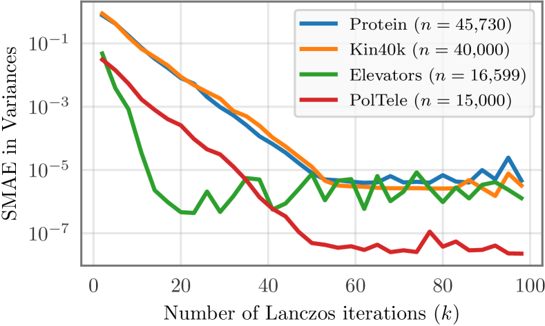
Figure 2: Predictive variance error as a function of the Lanczos iterations (KISS-GP model, $m=10,\!000$, Protein, Kin40k, PoleTele, Elevators UCI datasets).

Accuracy vs. Lanczos iterations.

In Figure 2, we measure the accuracy of LOVE as a function of the number of Lanczos iterations ($k$). We train a KISS-GP model with a deep RBF kernel on the four largest datasets from Table 2, using the setup described above. We measure the SMAE of KISS-GP/LOVE’s predictive variances compared against the standard KISS-GP variances (KISS-GP w/o LOVE). As seen in Figure 2, error decreases exponentially with the number of Lanczos iterations, up until roughly $50$ iterations. After roughly $50$ iterations, the error levels off, though this may be an artifact of floating-point precision (which may also cause small subsequent fluctuations). Recall that $k$ also corresponds with the rank of the $R$ and $R^{\prime}$ matrices in (10).

4.2 Sampling

We evaluate the quality of posterior samples drawn with KISS-GP/LOVE as described in Section 3.3. We compare these samples to three baselines: sampling from an Exact GP using the Cholesky decomposition, sampling from an SGPR model with Cholesky, and sampling with random Fourier features (Rahimi & Recht, 2008) – a method commonly used in Bayesian optimization (Hernández-Lobato et al., 2014; Wang & Jegelka, 2017). The KISS-GP/LOVE and SGPR models use the same architecture as described in the previous section. For Fourier features, we use 5000 random features – the maximum number of features that could be used without exhausting available GPU memory. We learn hyperparameters on the Exact GP and then use the same hyperparameters for the all methods.

We test on the two largest UCI datasets which can still be solved exactly (PolTele, Eleveators) and two Bayesian optimization benchmark functions (Eggholder – 2 dimensional, and Styblinski-Tang – 10 dimensional). The UCI datasets use the same training procedure as in the previous section. For the BayesOpt functions, we evaluate the model after 100 queries of max value entropy search (Wang & Jegelka, 2017). We use a standard (non-deep) RBF kernel for Eggholder, and for Syblinski-Tang we use the additive kernel decomposition suggested by Kandasamy et al. (2015).

Sample accuracy.

In Table 3 we evaluate the accuracy of the different sampling methods. We draw $s\!=\!1000$ samples at $t\!=\!10,\!000$ test locations and compare the sample covariance matrix with the true posterior covariance matrix $k_{f\mid\mathcal{D}}(X^{*},X^{*^{\prime}})$ in terms of element-wise mean absolute error. It is worth noting that all methods incur some error – even when sampling with an Exact GP. Nevertheless, Exact GPs, SGPR, and LOVE produce very accurate sample covariance matrices. In particular, Exact GPs and LOVE achieve between 1 and 3 orders of magnitude less error than the random Fourier Feature method.

Speed.

Though LOVE, Exact GPs, and SGPR have similar sample accuracies, LOVE is much faster. Even when accounting for LOVE’s pre-computation time (i.e. sampling “from scratch”), LOVE is comparable to Fourier features and SGPR in terms of speed. At test time (i.e. after pre-computation), LOVE is up to $18,\!000$ times faster than Exact.

Bayesian optimization.

Many acquisition functions in Bayesian optimization rely on sampling from the posterior GP. For example, max-value entropy search (Wang & Jegelka, 2017) draws samples from a posterior GP in order to estimate the function’s maximum value $p(y^{*}\!\mid\!\mathcal{D})$. The corresponding maximum location distribution, $p(x^{*}\!\mid\!\mathcal{D})$, is also the primary distribution of interest in predictive entropy search (Hernández-Lobato et al., 2014).

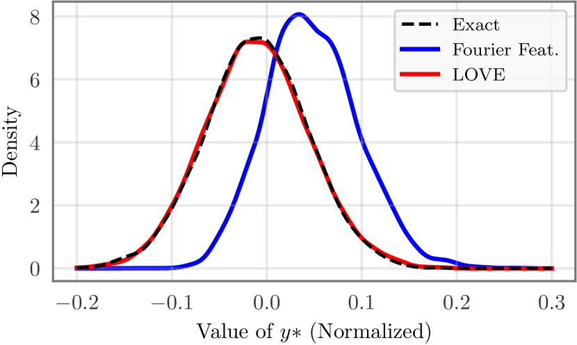
Figure 3: A density estimation plot of the predictive maximum distribution, $p(y^{*}\!\mid\!\mathcal{D})$ for the (normalized) Eggholder function after 100 iterations of BayesOpt. Samples drawn with KISS-GP/LOVE closely match samples drawn using an Exact GP. See Wang & Jegelka (2017) for details.

In Figure 3, we visualize each method’s sampled distribution of $p(y^{*}\!\mid\!\mathcal{D})$ for the Eggholder benchmark. We plot kernel density estimates of the sampled maximum value distributions after $100$ BayesOpt iterations. Since the Exact GP sampling method uses the exact Cholesky decomposition, its sampled max-value distribution can be considered closest to ground truth. The Fourier feature sampled distribution differs significantly. In contrast, LOVE’s sampled distribution very closely resembles the Exact GP distribution, yet LOVE is $700\times$ faster than the Exact GP on this dataset (Table 3).

5 Discussion, Related Work, and Conclusion

This paper has primarily focused on LOVE in the context of KISS-GP as its underlying inducing point method. This is because of KISS-GP’s accuracy, its efficient MVMs, and its constant asymptotic complexities when used with LOVE. However, LOVE and MVM inference are fully compatible with other inducing point techniques as well. Many inducing point methods make use of the subset of regressors (SOR) kernel approximation $K_{XX}\approx K_{XU}K_{UU}^{-1}K_{UX}$, optionally with a diagonal correction (Snelson & Ghahramani, 2006), and focus on the problem of learning the inducing point locations (Quiñonero-Candela & Rasmussen, 2005; Titsias, 2009). After $\mathcal{O}(m^{3})$ work to Cholesky decompose $\mathcal{O}(K_{UU})$, this approximate kernel affords $\mathcal{O}(n+m^{2})$ MVMs. One could apply LOVE to these methods and compute a test-invariant cache in $\mathcal{O}(knm+km^{2})$ time, and then compute single predictive covariances in $\mathcal{O}(mk)$ time. We note that, since these inducing point methods make a rank $m$ approximation to the kernel, setting $k\!=\!m$ produces exact solves with Lanczos decomposition, and recovers the $\mathcal{O}(nm^{2})$ precomputation time and $\mathcal{O}(m^{2})$ prediction time of these methods.

Ensuring Lanczos solves are accurate.

Given a matrix $\widehat{K}_{XX}$, the Lanczos decomposition $Q_{k}T_{k}Q_{k}^{\top}$ is designed to approximate the solve $\widehat{K}_{XX}^{-1}\mathbf{b}$, where $\mathbf{b}$ is the first column of $Q_{k}$. As argued in Section 2.2, the $Q_{k}$ and $T_{k}$ can usually be re-used to approximate the solves $\widehat{K}_{XX}^{-1}(W_{X}^{\top}K_{UU})\approx Q_{k}T_{k}^{-1}Q_{k}^{\top}(W_{X}^{\top}K_{UU})$. This property of the Lanczos decomposition is why LOVE can compute fast predictive variances. While this method usually produces accurate solves, the solves will not be accurate if some columns of $(W^{\top}_{X}K_{UU})$ are (nearly) orthogonal to the columns of $Q_{k}$. In this scenario, Saad (1987) suggests that the additional Lanczos iterations with a new probe vector will correct these errors. In practice, we find that these countermeasures are almost never necessary with LOVE – the Lanczos solves are almost always accurate.

Numerical stability of Lanczos.

A practical concern for LOVE is round-off errors that may affect the Lanczos algorithm. In particular it is common in floating point arithmetic for the vectors of $Q$ to lose orthogonality (Paige, 1970; Simon, 1984; Golub & Van Loan, 2012), resulting in an incorrect decomposition. To correct for this, several methods such as full reorthogonalization and partial or selective reorthogonalization exist (Golub & Van Loan, 2012). In our implementation, we use full reorthogonalization when a loss of orthogonality is detected. In practice, the cost of this correction is absorbed by the parallel performance of the GPU and does not impact the final running time.

Conclusion.

Whereas the running times of previous state-of-the-art methods depend on dataset size, LOVE provides constant time and near-exact predictive variances. In addition to providing scalable predictions, LOVE’s fast sampling procedure has the potential to dramatically simplify a variety of GP applications such as (e.g., Deisenroth & Rasmussen, 2011; Hernández-Lobato et al., 2014; Wang & Jegelka, 2017). These applications require fast posterior samples, and have previously relied on parametric approximations or finite basis approaches for approximate sampling (e.g., Deisenroth & Rasmussen, 2011; Wang & Jegelka, 2017). The ability for LOVE to obtain samples in linear time and variances in constant time will improve these applications, and may even unlock entirely new applications for Gaussian processes in the future.

References

- Asuncion & Newman (2007) Asuncion, A. and Newman, D. Uci machine learning repository. https://archive.ics.uci.edu/ml/, 2007. Last accessed: 2018-02-05.
- Cunningham et al. (2008) Cunningham, J. P., Shenoy, K. V., and Sahani, M. Fast gaussian process methods for point process intensity estimation. In ICML, pp. 192–199. ACM, 2008.
- Deisenroth & Rasmussen (2011) Deisenroth, M. and Rasmussen, C. E. Pilco: A model-based and data-efficient approach to policy search. In ICML, pp. 465–472, 2011.
- Deisenroth et al. (2015) Deisenroth, M. P., Fox, D., and Rasmussen, C. E. Gaussian processes for data-efficient learning in robotics and control. IEEE Transactions on Pattern Analysis and Machine Intelligence, 37(2):408–423, 2015.
- Demmel (1997) Demmel, J. W. Applied numerical linear algebra, volume 56. Siam, 1997.
- Dong et al. (2017) Dong, K., Eriksson, D., Nickisch, H., Bindel, D., and Wilson, A. G. Scalable log determinants for gaussian process kernel learning. In NIPS, 2017.
- Doshi-Velez & Kim (2017) Doshi-Velez, F. and Kim, B. A roadmap for a rigorous science of interpretability. arXiv preprint arXiv:1702.08608, 2017.
- Frazier et al. (2009) Frazier, P., Powell, W., and Dayanik, S. The knowledge-gradient policy for correlated normal beliefs. INFORMS journal on Computing, 21(4):599–613, 2009.
- Gardner et al. (2017) Gardner, J., Guo, C., Weinberger, K., Garnett, R., and Grosse, R. Discovering and exploiting additive structure for bayesian optimization. In AISTATS, pp. 1311–1319, 2017.
- Gardner et al. (2018) Gardner, J. R., Pleiss, G., Wu, R., Weinberger, K. Q., and Wilson, A. G. Product kernel interpolation for scalable gaussian processes. In AISTATS, 2018.
- Golub & Van Loan (2012) Golub, G. H. and Van Loan, C. F. Matrix computations, volume 3. JHU Press, 2012.
- Hensman et al. (2013) Hensman, J., Fusi, N., and Lawrence, N. D. Gaussian processes for big data. arXiv preprint arXiv:1309.6835, 2013.
- Hernández-Lobato et al. (2014) Hernández-Lobato, J. M., Hoffman, M. W., and Ghahramani, Z. Predictive entropy search for efficient global optimization of black-box functions. In NIPS, pp. 918–926, 2014.
- Hyndman (2005) Hyndman, R. J. Time series data library. http://www-personal.buseco.monash.edu.au/~hyndman/TSDL/, 2005. Last accessed: 2018-02-05.
- Kandasamy et al. (2015) Kandasamy, K., Schneider, J., and Póczos, B. High dimensional bayesian optimisation and bandits via additive models. In International Conference on Machine Learning, pp. 295–304, 2015.
- Keys (1981) Keys, R. Cubic convolution interpolation for digital image processing. IEEE transactions on acoustics, speech, and signal processing, 29(6):1153–1160, 1981.
- Kingma & Ba (2015) Kingma, D. P. and Ba, J. Adam: A method for stochastic optimization. In ICLR, 2015.
- Lanczos (1950) Lanczos, C. An iteration method for the solution of the eigenvalue problem of linear differential and integral operators. United States Governm. Press Office Los Angeles, CA, 1950.
- Loan (1999) Loan, C. F. V. Introduction to scientific computing: a matrix-vector approach using MATLAB. Prentice Hall PTR, 1999.
- Matthews et al. (2017) Matthews, A. G. d. G., van der Wilk, M., Nickson, T., Fujii, K., Boukouvalas, A., León-Villagrá, P., Ghahramani, Z., and Hensman, J. Gpflow: A gaussian process library using tensorflow. Journal of Machine Learning Research, 18(40):1–6, 2017.
- Nickisch et al. (2009) Nickisch, H., Pohmann, R., Schölkopf, B., and Seeger, M. Bayesian experimental design of magnetic resonance imaging sequences. In Advances in Neural Information Processing Systems, pp. 1441–1448, 2009.
- Paige (1970) Paige, C. Practical use of the symmetric lanczos process with re-orthogonalization. BIT Numerical Mathematics, 10(2):183–195, 1970.
- Papandreou & Yuille (2011) Papandreou, G. and Yuille, A. L. Efficient variational inference in large-scale bayesian compressed sensing. In ICCV Workshops, 2011.
- Parlett (1980) Parlett, B. N. A new look at the lanczos algorithm for solving symmetric systems of linear equations. Linear algebra and its applications, 29:323–346, 1980.
- Quiñonero-Candela & Rasmussen (2005) Quiñonero-Candela, J. and Rasmussen, C. E. A unifying view of sparse approximate gaussian process regression. Journal of Machine Learning Research, 6(Dec):1939–1959, 2005.
- Rahimi & Recht (2008) Rahimi, A. and Recht, B. Random features for large-scale kernel machines. In Advances in neural information processing systems, pp. 1177–1184, 2008.
- Rasmussen & Williams (2006) Rasmussen, C. E. and Williams, C. K. Gaussian processes for machine learning, volume 1. MIT press Cambridge, 2006.
- Saad (1987) Saad, Y. On the lanczos method for solving symmetric linear systems with several right-hand sides. Mathematics of computation, 48(178):651–662, 1987.
- Saatçi (2012) Saatçi, Y. Scalable inference for structured Gaussian process models. PhD thesis, University of Cambridge, 2012.
- Schneider & Willsky (2001) Schneider, M. K. and Willsky, A. S. Krylov subspace estimation. SIAM Journal on Scientific Computing, 22(5):1840–1864, 2001.
- Schulam & Saria (2017) Schulam, P. and Saria, S. What-if reasoning with counterfactual gaussian processes. In NIPS, 2017.
- Simon (1984) Simon, H. D. The lanczos algorithm with partial reorthogonalization. Mathematics of Computation, 42(165):115–142, 1984.
- Snelson & Ghahramani (2006) Snelson, E. and Ghahramani, Z. Sparse Gaussian processes using pseudo-inputs. In NIPS, pp. 1257–1264, 2006.
- Snoek et al. (2012) Snoek, J., Larochelle, H., and Adams, R. P. Practical bayesian optimization of machine learning algorithms. In Advances in neural information processing systems, pp. 2951–2959, 2012.
- Titsias (2009) Titsias, M. K. Variational learning of inducing variables in sparse gaussian processes. In AISTATS, pp. 567–574, 2009.
- Wang & Jegelka (2017) Wang, Z. and Jegelka, S. Max-value entropy search for efficient bayesian optimization. In ICML, 2017.
- Wang et al. (2017) Wang, Z., Li, C., Jegelka, S., and Kohli, P. Batched high-dimensional bayesian optimization via structural kernel learning. arXiv preprint arXiv:1703.01973, 2017.
- Wilson & Adams (2013) Wilson, A. and Adams, R. Gaussian process kernels for pattern discovery and extrapolation. In ICML, pp. 1067–1075, 2013.
- Wilson & Nickisch (2015) Wilson, A. G. and Nickisch, H. Kernel interpolation for scalable structured gaussian processes (kiss-gp). In ICML, pp. 1775–1784, 2015.
- Wilson et al. (2015) Wilson, A. G., Dann, C., and Nickisch, H. Thoughts on massively scalable gaussian processes. arXiv preprint arXiv:1511.01870, 2015.
- Wilson et al. (2016a) Wilson, A. G., Hu, Z., Salakhutdinov, R., and Xing, E. P. Deep kernel learning. In AISTATS, pp. 370–378, 2016a.
- Wilson et al. (2016b) Wilson, A. G., Hu, Z., Salakhutdinov, R. R., and Xing, E. P. Stochastic variational deep kernel learning. In Advances in Neural Information Processing Systems, pp. 2586–2594, 2016b.
- Zhou et al. (2017) Zhou, J., Arshad, S. Z., Luo, S., and Chen, F. Effects of uncertainty and cognitive load on user trust in predictive decision making. In IFIP Conference on Human-Computer Interaction, pp. 23–39. Springer, 2017.