A Family of Second-Order Energy-Stable Schemes for Cahn-Hilliard Type Equations

Abstract

We focus on the numerical approximation of the Cahn-Hilliard type equations, and present a family of second-order unconditionally energy-stable schemes. By reformulating the equation into an equivalent system employing a scalar auxiliary variable, we approximate the system at the time step $(n+\theta)$ ($n$ denoting the time step index and $\theta$ is a real-valued parameter), and devise a family of corresponding approximations that are second-order accurate and unconditionally energy stable. This family of approximations contains the often-used Crank-Nicolson scheme and the second-order backward differentiation formula as particular cases. We further develop an efficient solution algorithm for the resultant discrete system of equations to overcome the difficulty caused by the unknown scalar auxiliary variable. The final algorithm requires only the solution of four de-coupled individual Helmholtz type equations within each time step, which involve only constant and time-independent coefficient matrices that can be pre-computed. A number of numerical examples are presented to demonstrate the performance of the family of schemes developed herein. We note that this family of second-order approximations can be readily applied to devise energy-stable schemes for other types of gradient flows when combined with the auxiliary variable approaches.

Keywords: Cahn-Hilliard equation; energy stability; unconditional stability; free energy; phase field; two-phase flow

1 Introduction

Diffuse interface or phase field approach AndersonMW1998 ; LowengrubT1998 ; LiuS2003 ; YueFLS2004 has become one of the main techniques for modeling and simulating two-phase and multiphase problems involving fluid interfaces and the effect of surface tensions. Cahn-Hilliard type equations CahnH1958 are one of the commonly encountered equations in such models for describing the evolution of the phase field functions. Indeed, with an appropriate free energy density form, the mass balance equations for the individual fluid components in a multicomponent mixture will reduce to the Cahn-Hilliard type equations HohenbergH1977 ; GurtinPV1996 ; AbelsGG2012 ; Dong2014 ; Dong2018 . Devising efficient numerical schemes for Cahn-Hilliard equations therefore has crucial implications to two-phase and multiphase problems, and this has attracted a sustained interest from the community TierraG2015 .

Nonlinearity and high spatial order (fourth order) are the main issues encountered when numerically solving the Cahn-Hilliard equations. The interfacial thickness scale parameter, when small, also exacts high mesh resolutions in numerical simulations. The energy stability property of a numerical scheme, when the computational cost is manageable, is a desirable feature for solving the Cahn-Hilliard equations. While other types (e.g. conditionally stable, semi-implicit) of schemes for the Cahn-Hilliard equation also exist in the literature (see e.g. BadalassiCB2003 ; YueFLS2004 ; DongS2012 ; Dong2014obc ; GonzalezT2013 ; Dong2017 , among others), in what follows we will focus on the energy-stable schemes in the review of literature.

The nonlinearity of Cahn-Hilliard equation is induced by the potential free energy density function. Ensuring discrete energy stability in a numerical scheme hinges on the treatment of the nonlinear term. Based on the strategies for treating the nonlinear term, existing energy stable schemes for the Cahn-Hilliard equations can be broadly classified into two categories: nonlinear schemes and linear schemes. Nonlinear schemes (see e.g. ElliotFM1989 ; Furihata2001 ; FengP2004 ; KimKL2004 ; MelloF2005 ; Feng2006 ; Wise2010 ; HuaLLW2011 ) entail the solution of a system of nonlinear algebraic equations within a time step after discretization. Convex splitting of the potential energy term and its variants are a popular approach to treat the nonlinear term in this category ElliotS1993 ; Eyre1998 . Other treatments include the midpoint approximation ElliotFM1989 ; LinLZ2007 , specially designed quadrature formulas GomezH2011 , and Taylor expansion approximations KimKL2004 of the potential term, among others. On the other hand, linear schemes (see e.g. ShenY2010 ; GonzalezT2013 ; Yang2016 ; ShenXY2018 ) involve only the solution of a system of linear algebraic equations after discretization, thanks to certain special treatment of the nonlinear term or the introduction of certain auxiliary variables. Adding a stabilization term that is equivalent to zero while using a potential energy with bounded second derivative and treating the nonlinear term explicitly ShenY2010 ; GonzalezT2013 is a widely used technique in this category. Using a Lagrange multiplier BadiaGG2011 ; GonzalezT2013 is another technique to derive unconditionally energy-stable schemes for the Cahn-Hilliard equation. The invariant energy quadratization (IEQ) Yang2016 is a general technique that generalizes the Lagrange multiplier approach and can be applied to a large class of free energy forms. IEQ introduces an auxiliary field function related to the square root of the potential free energy density function together with a dynamic equation for this auxiliary variable, and allows one to devise schemes to ensure the energy stability relatively easily. The IEQ method gives rise to a system of linear algebraic equations involving time-dependent coefficient matrices after discretization. A further development of the auxiliary variable strategy is introduced in ShenXY2018 very recently, in which an auxiliary variable, which is a scalar value rather than a field function, related to the square root of the total potential energy integral has been employed. The scalar auxiliary variable (SAV) method retains the main advantage of IEQ, and further can lead to a constant coefficient matrix for the resultant linear algebraic system of equations after discretization.

In the current work we focus on the numerical approximation of the Cahn-Hilliard equation, reformulated using the scalar auxiliary variable appproach. We present a family of second-order accurate linear schemes for the system, and show that this family of schemes is unconditionally energy-stable. This family of approximations contains the Crank-Nicolson scheme (or trapezoidal rule) and the second-order backward differentiation formula (BDF2) as particular cases. The key idea of the schemes lies in enforcing the system of equations at the time step $(n+\theta)$, where $n$ is the time step index and $\theta$ is a real-valued parameter ($\frac{1}{2}\leqslant\theta\leqslant\frac{3}{2}$), and then devising appropriate corresponding approximations at $(n+\theta)$ with second-order accuracy that guarantee the energy stability of the system. We further present an efficient solution algorithm for the discretized system of equations to overcome the numerical difficulty induced by the unknown scalar auxiliary variable. Our overall algorithm only requires the computation of four de-coupled individual Helmholtz type equations within a time step, which involve constant coefficient matrices that can be pre-computed.

The novelties of this paper lie in two aspects: (i) the family of second-order accurate energy-stable schemes, and (ii) the efficient solution algorithm for the discrete system resulting from the Cahn-Hilliard type equations.

While we only consider the numerical approximation of the Cahn-Hilliard equation in this work, we would like to point out that the family of second-order energy-stable approximations herein are general, and are readily applicable to other types of equations resulting from gradient flows for designing energy-stable schemes when combined with the IEQ or SAV strategy.

The rest of this paper is structured as follows. In Section 2 we discuss the SAV reformulation of the Cahn-Hilliard equation, and present the family of second-order energy-stable approximations of the reformulated system of equations. We will also present an efficient solution algorithm for the discretized equations and an implementation of the algorithm based on the $C^{0}$-continuous spectral element method for spatial discretizations. In Section 3 we test the performance of the algorithms using several representative numerical examples, and demonstrate numerically the stability of computations with large time step sizes. Section 4 concludes the presentation with some closing remarks. The Appendices A and B provide proofs for the energy stability and another property of the presented family of schemes.

2 A Family of Second-Order Energy-Stable Schemes

2.1 Cahn-Hilliard Equation, Boundary Conditions, and Transformed System

Consider a domain $\Omega$ in two or three dimensions, whose boundary is denoted by $\partial\Omega$, and the Cahn-Hilliard equation CahnH1958 with a source term within this domain:

$$\frac{\partial\phi}{\partial t}=m\nabla^{2}\left[-\lambda\nabla^{2}\phi+h(\phi)\right]+g(\mathbf{x},t)$$ (1)

where $\phi(\mathbf{x},t)$ ($\phi\in[-1,1]$) is the phase field function, $m>0$ is the mobility and assumed to be a constant in this work, and $\mathbf{x}$ and $t$ denote the spatial coordinates and time. $g(\mathbf{x},t)$ is a prescribed source term for the purpose of numerical testing (for convergence rates) only, and will be set to $g(\mathbf{x},t)=0$ in actual simulations. $\lambda$ is the mixing energy density coefficient and is related to other physical parameters, e.g. for two-phase flow problems it is given by (see YueFLS2004 ) $\lambda=\frac{3}{2\sqrt{2}}\sigma\eta,$ where $\sigma$ is the surface tension and $\eta$ is the characteristic interfacial thickness. The nonlinear term $h(\phi)$ is given by $h(\phi)=\frac{dF(\phi)}{d\phi}$, where $F(\phi)$ is the potential free energy density function of the system. A double-well potential is often used for $F(\phi)$, in the form $F(\phi)=\frac{\lambda}{4\eta^{2}}(\phi^{2}-1)^{2},$ and this form will be used for the numerical tests in Section 3.

We consider the wall-type boundary with a neutral wettability (i.e. $90^{0}$ contact angle) for $\partial\Omega$, characterized by the following boundary conditions Jacqmin1999 ; YueZF2010 ; Dong2012

$$\mathbf{n}\cdot\nabla\left[-\lambda\nabla^{2}\phi+h(\phi)\right]=g_{a}(\mathbf{x},t),\quad\text{on}\ \partial\Omega$$ (2a)

$$\mathbf{n}\cdot\nabla\phi=g_{b}(\mathbf{x},t),\quad\text{on}\ \partial\Omega$$ (2b)

where $\mathbf{n}$ is the outward-pointing unit vector normal to $\partial\Omega$. $g_{a}(\mathbf{x},t)$ and $g_{b}(\mathbf{x},t)$ are prescribed source terms for the purpose of numerical testing only, and will be set to $g_{a}=0$ and $g_{b}=0$ in actual simulations.

The system consisting of the equation (1) and the boundary conditions (2a) and (2b), with $g=0$, $g_{a}=0$ and $g_{b}=0$, satisfies the following energy balance equation:

$$\frac{\partial}{\partial t}\int_{\Omega}\left(\frac{\lambda}{2}\nabla\phi\cdot\nabla\phi+F(\phi)\right)=-m\int_{\Omega}\left|\nabla\left[-\lambda\nabla^{2}\phi+h(\phi)\right]\right|^{2}.$$ (3)

This system is to be supplemented by the following initial condition

$$\phi(\mathbf{x},0)=\phi_{in}(\mathbf{x})$$ (4)

where $\phi_{in}(\mathbf{x})$ denotes the initial phase field distribution.

We next reformulate this system of equations and boundary conditions into a modified equivalent system, by introducing an auxiliary variable associated with the total potential energy in a way similar to ShenXY2018 . Define the total potential free energy $E(t)$ by

$$E(t)=E[\phi]=C_{0}+\int_{\Omega}F(\phi)$$ (5)

where $C_{0}$ is a chosen constant such that $E(t)>0$ for all $0\leqslant t\leqslant T$ ($T$ denoting the period of time to find the solution for). For all the numerical experiments presented in the current work we employ $C_{0}=0$ in the simulations. It is important to note that $E[\phi]$ as defined above is a scalar value, not a field function. We define an auxiliary variable $r(t)$ by

$$r(t)=\sqrt{E(t)}.$$ (6)

Then $r(t)$ satisfies the dynamic equation

$$\frac{dr}{dt}=\frac{1}{2\sqrt{E[\phi]}}\int_{\Omega}h(\phi)\frac{\partial\phi}{\partial t},$$ (7)

We re-write the Cahn-Hilliard equation (1) into an equivalent form

$$\frac{\partial\phi}{\partial t}=m\nabla^{2}\mathscr{H}+g,$$ (8a)

$$\mathscr{H}=-\lambda\nabla^{2}\phi+\frac{r(t)}{\sqrt{E[\phi]}}h(\phi),$$ (8b)

where the definition (6) has been used. The boundary conditions (2a) is also re-written into an equivalent form

$$\mathbf{n}\cdot\nabla\left[-\lambda\nabla^{2}\phi+\frac{r(t)}{\sqrt{E[\phi]}}h(\phi)\right]=g_{a},\quad\text{on}\ \partial\Omega,$$ (9a)

The system consisting of equations (8a)–(8b) and (7), the boundary conditions (9a) and (2b), and the initial conditions of (4) and the following

$$\begin{split}&r(0)=\sqrt{E[\phi_{in}]}=\left[\int_{\Omega}F(\phi_{in})+C_{0}\right]^{1/2},\end{split}$$ (10)

is equivalent to the original system consisting of equations (1), (2a)–(2b) and (4).

2.2 A Family of Second-Order Energy-Stable Approximations

We focus on the numerical approximation of the reformulated equivalent system consisting of equations (8a)–(8b) and (7), the boundary conditions (9a) and (2b), and the initial conditions (4) and (10). We present a family of second-order energy-stable schemes for this system that allows for a very efficient implementation.

Let $n\geqslant 0$ denote the time step index, and $(\cdot)^{n}$ represent the variable $(\cdot)$ at time step $n$, corresponding to the time $t=n\Delta t$, where $\Delta t$ is the time step size.

Let $\theta$ ($\frac{1}{2}\leqslant\theta\leqslant\frac{3}{2}$) denote a real-valued parameter. We approximate the variables at time step $(n+\theta)$ (corresponding to time $(n+\theta)\Delta t$) as follows with a scheme of second-order accuracy in time ($\chi$ denoting a generic variable below),

$$\left.\frac{\partial\chi}{\partial t}\right|^{n+\theta}=\frac{1}{\Delta t}\left[\left(\theta+\frac{1}{2}\right)\chi^{n+1}-2\theta\chi^{n}+\left(\theta-\frac{1}{2}\right)\chi^{n-1}\right],$$ (11a)

$$\chi^{n+\theta}=\left[\theta\left(\frac{5}{2}-\theta\right)-\frac{1}{2}\right]\chi^{n+1}+2(1-\theta)^{2}\chi^{n}+\left(\theta-\frac{1}{2}\right)(1-\theta)\chi^{n-1},$$ (11b)

$$\bar{\chi}^{n+\theta}=(1+\theta)\chi^{n}-\theta\chi^{n-1}.$$ (11c)

In the above $\chi^{n+\theta}$ and $\bar{\chi}^{n+\theta}$ are respectively an implicit and an explicit approximation of $\chi$ at time step $(n+\theta)$. The 2nd-order temporal accuracy of these approximations can be verified by Taylor expansions in a straightforward fashion. The implicit approximation $\chi^{n+\theta}$ given in (11b) is critical to the energy stability of the current family of schemes, due to the following crucial property:

$$\begin{split}&\chi^{n+\theta}\left[\left(\theta+\frac{1}{2}\right)\chi^{n+1}-2\theta\chi^{n}+\left(\theta-\frac{1}{2}\right)\chi^{n-1}\right]\\ &\quad=\frac{1}{2}\theta\left(\theta-\frac{1}{2}\right)(3-2\theta)\left|\chi^{n+1}-2\chi^{n}+\chi^{n-1}\right|^{2}+\frac{1}{2}\left(\frac{3}{2}-\theta\right)\left(\left|\chi^{n+1}\right|^{2}-\left|\chi^{n}\right|^{2}\right)\\ &\qquad+\frac{1}{2}\left(\theta-\frac{1}{2}\right)\left(\left|2\chi^{n+1}-\chi^{n}\right|^{2}-\left|2\chi^{n}-\chi^{n-1}\right|^{2}\right).\end{split}$$ (12)

This property can be verified by elementary manipulations. Note that the usual 2nd-order implicit approximation, $\chi^{n+\theta}=\theta\chi^{n+1}+(1-\theta)\chi^{n},$ cannot guarantee the energy stability with $\frac{1}{2}<\theta<1$. The family of approximations given by (11a)–(11c) contains the often-used 2nd-order backward differentiation formula (or BDF2, corresponding to $\theta=1$) and the Crank-Nicolson approximation (corresponding to $\theta=1/2$).

Given $(\phi^{n},r^{n})$, we compute $(\phi^{n+1},r^{n+1})$ by enforcing the system consisting of (7)–(9a) and (2b) at time step $(n+\theta)$ and using the above approximations (11a)–(11c), as follows,

$$\frac{\left(\theta+\frac{1}{2}\right)\phi^{n+1}-2\theta\phi^{n}+\left(\theta-\frac{1}{2}\right)\phi^{n-1}}{\Delta t}=m\nabla^{2}\mathscr{H}^{n+\theta}+g^{n+\theta},$$ (13a)

$$\mathscr{H}^{n+\theta}=-\lambda\nabla^{2}\phi^{n+\theta}+S(\phi^{n+1}-2\phi^{n}+\phi^{n-1})+\frac{r^{n+\theta}}{\sqrt{E[\bar{\phi}^{n+\theta}]}}h(\bar{\phi}^{n+\theta}),$$ (13b)

$$\frac{\left(\theta+\frac{1}{2}\right)r^{n+1}-2\theta r^{n}+\left(\theta-\frac{1}{2}\right)r^{n-1}}{\Delta t}=\int_{\Omega}\frac{h(\bar{\phi}^{n+\theta})}{2\sqrt{E[\bar{\phi}^{n+\theta}]}}\frac{\left(\theta+\frac{1}{2}\right)\phi^{n+1}-2\theta\phi^{n}+\left(\theta-\frac{1}{2}\right)\phi^{n-1}}{\Delta t},$$ (13c)

$$\mathbf{n}\cdot\nabla\left[-\lambda\nabla^{2}\phi^{n+\theta}+S(\phi^{n+1}-2\phi^{n}+\phi^{n-1})+\frac{r^{n+\theta}}{\sqrt{E[\bar{\phi}^{n+\theta}]}}h(\bar{\phi}^{n+\theta})\right]=g_{a}^{n+\theta},\quad\text{on}\ \partial\Omega,$$ (13d)

$$\mathbf{n}\cdot\nabla\phi^{n+\theta}=g_{b}^{n+\theta},\quad\text{on}\ \partial\Omega.$$ (13e)

In the above equations (13b) and (13d), $S\geqslant 0$ is a chosen constant that satisfies a condition to be specified later. Note that because $\phi^{n+1}-2\phi^{n}+\phi^{n-1}={\cal{O}}{(\Delta t)^{2}}$ the extra term $S(\phi^{n+1}-2\phi^{n}+\phi^{n-1})$ in (13b) and (13d) does not spoil the second-order accuracy of the overall scheme. In the above equations the variables $\phi^{n+\theta}$, $\bar{\phi}^{n+\theta}$, and $r^{n+\theta}$ are given by the equations (11b) and (11c). $g^{n+\theta}$, $g_{a}^{n+\theta}$ and $g_{b}^{n+\theta}$ are the prescribed functions $g(\mathbf{x},t)$, $g_{a}(\mathbf{x},t)$ and $g_{b}(\mathbf{x},t)$ evaluated at time $t=(n+\theta)\Delta t$, respectively.

The above scheme has the following property:

Theorem 2.1.

The scheme consisting of equations (13a)–(13e), in the absence of the source terms (i.e. $g=0$, $g_{a}=0$ and $g_{b}=0$), satisfies the discrete energy balance equation for $\frac{1}{2}\leqslant\theta\leqslant\frac{3}{2}$ and $S\geqslant 0$,

$$\begin{split}&W^{n+1}-W^{n}+\theta\left(\theta-\frac{1}{2}\right)(3-2\theta)\left(|r^{n+1}-2r^{n}+r^{n-1}|^{2}\right.\\ &\qquad\left.+\int_{\Omega}\frac{\lambda}{2}\left|\nabla\phi^{n+1}-2\nabla\phi^{n}+\nabla\phi^{n-1}\right|^{2}\right)+\theta S\int_{\Omega}\left|\phi^{n+1}-2\phi^{n}+\phi^{n-1}\right|^{2}\\ &=-m\Delta t\int_{\Omega}\left|\nabla\mathscr{H}^{n+\theta}\right|^{2}\end{split}$$ (14)

where

$$\begin{split}W^{n}=&\left(\frac{3}{2}-\theta\right)\left(|r^{n}|^{2}+\int_{\Omega}\frac{\lambda}{2}\left|\nabla\phi^{n}\right|^{2}\right)\\ &+\left(\theta-\frac{1}{2}\right)\left(\left|2r^{n}-r^{n-1}\right|^{2}+\int_{\Omega}\frac{\lambda}{2}\left|2\nabla\phi^{n}-\nabla\phi^{n-1}\right|^{2}\right)\\ &+\frac{S}{2}\int_{\Omega}\left|\phi^{n}-\phi^{n-1}\right|^{2}.\end{split}$$ (15)

A proof of this theorem is provided in the Appendix A.

Remark 1.

Based on this theorem the scheme given by equations (13a)–(13e) constitutes a family of unconditionally stable algorithms for $\frac{1}{2}\leqslant\theta\leqslant\frac{3}{2}$. Note that this energy stability property holds regardless of the specific form of the potential free energy density $F(\phi)$, as long as it is such that an appropriate constant $C_{0}$ in (5) can be chosen to ensure $E(t)>0$ for $0\leqslant t\leqslant T$.

Remark 2.

The first term on the right hand side of (12) determines the dissipativeness of the approximations (11a)–(11b). The algorithm with $\theta=\frac{2}{3}+\frac{\sqrt{7}}{6}\approx 1.11$ is the most dissipative among this family of approximations, while both $\theta=\frac{1}{2}$ (Crank-Nicolson) and $\theta=\frac{3}{2}$ are non-dissipative. In terms of numerical dissipation, BDF2 ($\theta=1$) is close to, but not as dissipative as, the scheme with $\theta=\frac{2}{3}+\frac{\sqrt{7}}{6}$.

Remark 3.

While we consider only the Cahn-Hilliard type equations in this work, the application of the family of 2nd-order approximations (11a)–(11c) is not limited to this class of equations. They can be readily applied to other types of equations describing gradient flows. For example, by combining these approximations and the auxiliary variable approaches of Yang2016 ; ShenXY2018 , one can derive a family of energy-stable schemes for a large class of gradient flows.

2.3 Efficient Solution Algorithm

The scheme represented by equations (13a)–(13e) involves integrals of the unknown field variable $\phi^{n+1}$ over the domain $\Omega$. Despite this apparent complication, the formulation allows for a simple and very efficient solution algorithm. We present such an algorithm below.

To facilitate subsequent discussions and make the representation more compact, we first introduce several notations ($\chi$ denoting a generic variable):

$$\gamma_{0}=\gamma_{0}(\theta)=\theta+\frac{1}{2},\qquad\omega_{0}=\omega_{0}(\theta)=\theta\left(\frac{5}{2}-\theta\right)-\frac{1}{2},$$ (16a)

$$\hat{\chi}=2\theta\chi^{n}-\left(\theta-\frac{1}{2}\right)\chi^{n-1},$$ (16b)

$$\tilde{\chi}=2(1-\theta)^{2}\chi^{n}+\left(\theta-\frac{1}{2}\right)(1-\theta)\chi^{n-1}.$$ (16c)

Then the approximations in (11a) and (11b) can be written as

$$\left.\frac{\partial\chi}{\partial t}\right|^{n+\theta}=\frac{\gamma_{0}\chi^{n+1}-\hat{\chi}}{\Delta t},$$ (17a)

$$\chi^{n+\theta}=\omega_{0}\chi^{n+1}+\tilde{\chi}.$$ (17b)

Combining equations (13a) and (13b) leads to

$$\frac{\gamma_{0}\phi^{n+1}-\hat{\phi}}{\Delta t}=m\nabla^{2}\left[-\lambda\nabla^{2}\left(\omega_{0}\phi^{n+1}+\tilde{\phi}\right)+S(\phi^{n+1}-\bar{\phi}^{n+1})+\left(\omega_{0}r^{n+1}+\tilde{r}\right)\frac{h(\bar{\phi}^{n+\theta})}{\sqrt{E[\bar{\phi}^{n+\theta}]}}\right]+g^{n+\theta}$$ (18)

where $\gamma_{0}$ and $\omega_{0}$ are given by (16a), $\hat{\phi}$ is defined by (16b), $\tilde{\phi}$ and $\tilde{r}$ are defined by (16c), $\bar{\phi}^{n+1}=2\phi^{n}-\phi^{n-1}$ based on equation (11c), and we have used equations (17a) and (17b). It is important to note that $\phi^{n+1}$, $\hat{\phi}$, $\tilde{\phi}$, $\bar{\phi}^{n+\theta}$, $\bar{\phi}^{n+1}$ are field functions, while $r^{n+1}$, $\tilde{r}$ and $E[\bar{\phi}^{n+\theta}]$ are scalar variables. Define

$$\begin{split}&b^{n}=\frac{h(\bar{\phi}^{n+\theta})}{\sqrt{E[\bar{\phi}^{n+\theta}]}},\qquad z^{n+1}=\int_{\Omega}b^{n}\phi^{n+1},\end{split}$$ (19)

Note that $b^{n}$ is a field function, and $z^{n+1}$ is a scalar variable. Equation (18) is then transformed into

$$\nabla^{2}(\nabla^{2}\phi^{n+1})-\frac{S}{\lambda\omega_{0}}\nabla^{2}\phi^{n+1}+\frac{\gamma_{0}}{\lambda\omega_{0}m\Delta t}\phi^{n+1}\\ =\frac{1}{\lambda\omega_{0}m}\left[g^{n+\theta}+\frac{\hat{\phi}}{\Delta t}\right]-\frac{S}{\lambda\omega_{0}}\nabla^{2}\bar{\phi}^{n+1}-\frac{1}{\omega_{0}}\nabla^{2}(\nabla^{2}\tilde{\phi})+\frac{\omega_{0}r^{n+1}+\tilde{r}}{\lambda\omega_{0}}\nabla^{2}b^{n}.$$ (20)

Equation (13c) can be written as $\gamma_{0}r^{n+1}-\hat{r}=\frac{1}{2}\int_{\Omega}b^{n}(\gamma_{0}\phi^{n+1}-\hat{\phi}),$ from which we get

$$r^{n+1}=\frac{1}{\gamma_{0}}\left(\hat{r}-\frac{1}{2}\int_{\Omega}b^{n}\hat{\phi}\right)+\frac{z^{n+1}}{2}$$ (21)

where $z^{n+1}$ is defined in (19) and involves the unknown field function $\phi^{n+1}$. In light of this expression, equation (20) is transformed into

$$\nabla^{2}(\nabla^{2}\phi^{n+1})-\frac{S}{\lambda\omega_{0}}\nabla^{2}\phi^{n+1}+\frac{\gamma_{0}}{\lambda\omega_{0}m\Delta t}\phi^{n+1}=Q^{n}+\frac{z^{n+1}}{2\lambda}\nabla^{2}b^{n},$$ (22)

where

$$Q^{n}=\frac{1}{\lambda\omega_{0}m}\left[g^{n+\theta}+\frac{\hat{\phi}}{\Delta t}\right]-\frac{S}{\lambda\omega_{0}}\nabla^{2}\bar{\phi}^{n+1}-\frac{1}{\omega_{0}}\nabla^{2}(\nabla^{2}\tilde{\phi})+\left[\frac{1}{\lambda\gamma_{0}}\left(\hat{r}-\frac{1}{2}\int_{\Omega}b^{n}\hat{\phi}\right)+\frac{\tilde{r}}{\lambda\omega_{0}}\right]\nabla^{2}b^{n}.$$ (23)

Barring the unknown scalar variable $z^{n+1}$, equation (22) is a fourth-order equation about $\phi^{n+1}$. The left-hand-side (LHS) of this equation can be reformulated into two de-coupled Helmholtz type equations (see e.g. YueFLS2004 ; DongS2012 ; Dong2012 ). By adding/subtracting a term $\alpha\nabla^{2}\phi^{n+1}$ ($\alpha$ denoting a constant to be determined) on the LHS of (22), we get

$$\nabla^{2}\left[\nabla^{2}\phi^{n+1}+\alpha\phi^{n+1}\right]-\left(\alpha+\frac{S}{\lambda\omega_{0}}\right)\left[\nabla^{2}\phi^{n+1}-\frac{\gamma_{0}}{\lambda\omega_{0}m\Delta t\left(\alpha+\frac{S}{\lambda\omega_{0}}\right)}\phi^{n+1}\right]=Q^{n}+\frac{z^{n+1}}{2\lambda}\nabla^{2}b^{n}.$$ (24)

By requiring $\alpha=-\frac{\gamma_{0}}{\lambda\omega_{0}m\Delta t\left(\alpha+\frac{S}{\lambda\omega_{0}}\right)},$ we can determine the constant $\alpha$,

$$\alpha=-\frac{S}{2\lambda\omega_{0}}\left[1-\sqrt{1-\frac{4\gamma_{0}}{\lambda\omega_{0}m\Delta t}\left(\frac{\lambda\omega_{0}}{S}\right)^{2}}\right]$$ (25)

with the requirement

$$S\geqslant\lambda\omega_{0}\sqrt{\frac{4\gamma_{0}}{\lambda\omega_{0}m\Delta t}}=\sqrt{\frac{4\gamma_{0}\lambda\omega_{0}}{m\Delta t}}.$$ (26)

This is the condition the chosen constant $S$ must satisfy.

Therefore, equation (24) can be transformed into the following equivalent form

$$\nabla^{2}\psi^{n+1}-\left(\alpha+\frac{S}{\lambda\omega_{0}}\right)\psi^{n+1}=Q^{n}+\frac{z^{n+1}}{2\lambda}\nabla^{2}b^{n},$$ (27a)

$$\nabla^{2}\phi^{n+1}+\alpha\phi^{n+1}=\psi^{n+1},$$ (27b)

where $\psi^{n+1}$ is an auxiliary field variable defined by (27b). Note that $\alpha<0$ and $\alpha+\frac{S}{\lambda\omega_{0}}>0$ under the condition (26) for $S$. It can also be noted that, if $z^{n+1}$ is known, then the two equations (27a) and (27b) are not coupled. One can first solve (27a) for $\psi^{n+1}$, and then solve (27b) for $\phi^{n+1}$. The unknown variable $z^{n+1}$, which depends on $\phi^{n+1}$, causes a complication in the solution of this system.

Let us now turn the attention to the boundary conditions. Equation (13e) can be written as

$$\mathbf{n}\cdot\nabla\phi^{n+1}=\frac{1}{\omega_{0}}\left(g_{b}^{n+\theta}-\mathbf{n}\cdot\nabla\tilde{\phi}\right)\quad\text{on}\ \partial\Omega.$$ (28)

Equation (13d) can be re-written as

$$-\lambda\mathbf{n}\cdot\nabla\left(\omega_{0}\nabla^{2}\phi^{n+1}+\nabla^{2}\tilde{\phi}\right)+S\mathbf{n}\cdot\nabla\left(\phi^{n+1}-\bar{\phi}^{n+1}\right)+\left(\omega_{0}r^{n+1}+\tilde{r}\right)\mathbf{n}\cdot\nabla b^{n}=g_{a}^{n+\theta},\quad\text{on}\ \partial\Omega.$$ (29)

In light of the equations (27b) and (21), we can transform this equation into

$$\mathbf{n}\cdot\nabla\psi^{n+1}=\left(\alpha+\frac{S}{\lambda\omega_{0}}\right)\mathbf{n}\cdot\nabla\phi^{n+1}-\frac{1}{\lambda\omega_{0}}\left(g_{a}^{n+\theta}+S\mathbf{n}\cdot\nabla\bar{\phi}^{n+1}\right)-\frac{1}{\omega_{0}}\mathbf{n}\cdot\nabla(\nabla^{2}\tilde{\phi})\\ +\left[\frac{\tilde{r}}{\lambda\omega_{0}}+\frac{1}{\lambda\gamma_{0}}\left(\hat{r}-\frac{1}{2}\int_{\Omega}b^{n}\hat{\phi}\right)+\frac{z^{n+1}}{2\lambda}\right]\mathbf{n}\cdot\nabla b^{n},\quad\text{on}\ \partial\Omega.$$ (30)

Substitute equation (28) into the above equation, and we have the boundary condition about $\psi^{n+1}$:

$$\mathbf{n}\cdot\nabla\psi^{n+1}=T^{n}+\frac{z^{n+1}}{2\lambda}\mathbf{n}\cdot\nabla b^{n},\quad\text{on}\ \partial\Omega,$$ (31)

where

$$T^{n}=\left(\alpha+\frac{S}{\lambda\omega_{0}}\right)\frac{1}{\omega_{0}}\left(g_{b}^{n+\theta}-\mathbf{n}\cdot\nabla\tilde{\phi}\right)-\frac{1}{\lambda\omega_{0}}\left(g_{a}^{n+\theta}+S\mathbf{n}\cdot\nabla\bar{\phi}^{n+1}\right)\\ -\frac{1}{\omega_{0}}\mathbf{n}\cdot\nabla(\nabla^{2}\tilde{\phi})+\left[\frac{\tilde{r}}{\lambda\omega_{0}}+\frac{1}{\lambda\gamma_{0}}\left(\hat{r}-\frac{1}{2}\int_{\Omega}b^{n}\hat{\phi}\right)\right]\mathbf{n}\cdot\nabla b^{n}.$$ (32)

Therefore, the original system of equations (13a)–(13e) has been reduced to the system consisting of equations (27a)–(27b), (31) and (28). After $\phi^{n+1}$ is solved from this system, $r^{n+1}$ can be computed based on equation (21).

To solve the system consisting of equations (27a)–(27b), (31) and (28), it is critical to note that the unknown variable $z^{n+1}$ involved therein is a scalar, not a field function, and that the equations are linear with respect to $\phi^{n+1}$, $\psi^{n+1}$, and $z^{n+1}$. In what follows we present an efficient algorithm for solving this system. We define two sets of field variables, $(\psi_{i}^{n+1},\phi_{i}^{n+1})$ ($i=1,2$), as follows:
For $\psi_{1}^{n+1}$:

$$\nabla^{2}\psi_{1}^{n+1}-\left(\alpha+\frac{S}{\lambda\omega_{0}}\right)\psi_{1}^{n+1}=Q^{n},$$ (33a)

$$\mathbf{n}\cdot\nabla\psi_{1}^{n+1}=T^{n},\quad\text{on}\ \partial\Omega.$$ (33b)

For $\phi_{1}^{n+1}$:

$$\nabla^{2}\phi_{1}^{n+1}+\alpha\phi_{1}^{n+1}=\psi_{1}^{n+1},$$ (34a)

$$\mathbf{n}\cdot\nabla\phi_{1}^{n+1}=\frac{1}{\omega_{0}}\left(g_{b}^{n+\theta}-\mathbf{n}\cdot\nabla\tilde{\phi}\right),\quad\text{on}\ \partial\Omega.$$ (34b)

For $\psi_{2}^{n+1}$:

$$\nabla^{2}\psi_{2}^{n+1}-\left(\alpha+\frac{S}{\lambda\omega_{0}}\right)\psi_{2}^{n+1}=\frac{1}{2\lambda}\nabla^{2}b^{n},$$ (35a)

$$\mathbf{n}\cdot\nabla\psi_{2}^{n+1}=\frac{1}{2\lambda}\mathbf{n}\cdot\nabla b^{n},\quad\text{on}\ \partial\Omega.$$ (35b)

For $\phi_{2}^{n+1}$:

$$\nabla^{2}\phi_{2}^{n+1}+\alpha\phi_{2}^{n+1}=\psi_{2}^{n+1},$$ (36a)

$$\mathbf{n}\cdot\nabla\phi_{2}^{n+1}=0,\quad\text{on}\ \partial\Omega.$$ (36b)

Then we have the following result.

Theorem 2.2.

For given scalar value $z^{n+1}$, the following field functions solve the system consisting of equations (27a)–(27b), (31) and (28):

$$\psi^{n+1}=\psi_{1}^{n+1}+z^{n+1}\psi_{2}^{n+1},$$ (37a)

$$\phi^{n+1}=\phi_{1}^{n+1}+z^{n+1}\phi_{2}^{n+1},$$ (37b)

where $(\psi_{i}^{n+1},\phi_{i}^{n+1})$ ($i=1,2$) are given by equations (33a)–(36b).

This theorem can be proved by straightforward substitutions and verifications.

We still need to determine the value for $z^{n+1}$. Substituting the expression $\phi^{n+1}$ in (37b) into the definition for $z^{n+1}$ in (19) results in

$$z^{n+1}=\frac{\int_{\Omega}b^{n}\phi_{1}^{n+1}}{1-\int_{\Omega}b^{n}\phi_{2}^{n+1}}.$$ (38)

We have the following result:

Theorem 2.3.

The $\phi_{2}^{n+1}$ defined by (35a)–(36b) satisfies the property,

$$\int_{\Omega}b^{n}\phi_{2}^{n+1}\leqslant 0.$$ (39)

A proof of this theorem is provided in Appendix B. Based on this theorem, $z^{n+1}$ given by (38) is well defined for any $\Delta t$.

Combining the above discussions, we arrive at the solution algorithm for solving the system consisting of equations (13a)–(13e). Given $(\phi^{n},r^{n})$, we compute $(\phi^{n+1},\nabla^{2}\phi^{n+1},r^{n+1})$ through the following steps:

1. Solve equations (33a)–(33b) for $\psi_{1}^{n+1}$;
   Solve equations (34a)–(34b) for $\phi_{1}^{n+1}$.

2. Solve equations (35a)–(35b) for $\psi_{2}^{n+1}$;
   Solve equations (36a)–(36b) for $\phi_{2}^{n+1}$.

3. Solve equations (38) for $z^{n+1}$.

4. Compute $\psi^{n+1}$ and $\phi^{n+1}$ based on equations (37a) and (37b), respectively.
   Compute $\nabla^{2}\phi^{n+1}$ as follows in light of equation (27b)

   $$\nabla^{2}\phi^{n+1}=\psi^{n+1}-\alpha\phi^{n+1}.$$ (40)

5. Compute $r^{n+1}$ based on equation (21).

Remark 4.

This algorithm involves only the solution of four de-coupled Helmholtz type equations within a time step. These Helmholtz equations involve only two distinct coefficient matrices after spatial discretization, and they are both constant coefficient matrices and can be pre-computed. No nonlinear algebraic solver is involved in this algorithm. Thanks to these characteristics, the family of second-order energy-stable schemes represented by (13a)–(13e) can be implemented in a very efficient fashion.

2.4 Implementation with $C^{0}$ Spectral Elements

The solution algorithm presented in the previous subsection can be implemented using any commonly-used method for the spatial discretization. In the current work we will employ $C^{0}$ continuous high-order spectral elements KarniadakisS2005 ; ZhengD2011 for spatial discretizations. We next consider the implementation of the algorithm using $C^{0}$ spectral elements. The discussions in this subsection without change also apply to implementations using low-order finite elements.

We will first derive the weak forms about $(\psi_{i}^{n+1},\phi_{i}^{n+1})$ ($i=1,2$) in the continuous space, and then specify the discrete function space for the spectral element approximations. In the process, certain terms involving derivatives of order two or higher will be dealt with appropriately so that all quantities involved in the weak formulation can be computed directly using $C^{0}$ elements in the discrete function space.

Let $\varphi(\mathbf{x})$ denote a test function. Taking the $L^{2}$ inner product between $\varphi$ and the equation (33a) leads to

$$\int_{\Omega}\nabla\psi_{1}^{n+1}\cdot\nabla\varphi+\left(\alpha+\frac{S}{\lambda\omega_{0}}\right)\int_{\Omega}\psi_{1}^{n+1}\varphi=-\int_{\Omega}Q^{n}\varphi+\int_{\partial\Omega}T^{n}\varphi,\quad\forall\varphi,$$ (41)

where we have used integration by part and the equation (33b). By substituting the $Q^{n}$ expression from (23) and $T^{n}$ expression from (32) into the RHS of the above equation and integration by part, we obtain the weak form about $\psi_{1}^{n+1}$,

$$\begin{split}&\int_{\Omega}\nabla\psi_{1}^{n+1}\cdot\nabla\varphi+\left(\alpha+\frac{S}{\lambda\omega_{0}}\right)\int_{\Omega}\psi_{1}^{n+1}\varphi\\ &=-\frac{1}{\lambda\omega_{0}m}\int_{\Omega}\left(g^{n+\theta}+\frac{\hat{\phi}}{\Delta t}\right)\varphi-\frac{S}{\lambda\omega_{0}}\int_{\Omega}\nabla\bar{\phi}^{n+1}\cdot\nabla\varphi-\frac{1}{\omega_{0}}\int_{\Omega}\nabla\left(\nabla^{2}\tilde{\phi}\right)\cdot\nabla\varphi-\frac{1}{\lambda\omega_{0}}\int_{\partial\Omega}g_{a}^{n+\theta}\varphi\\ &\quad+\left[\frac{1}{\lambda\gamma_{0}}\left(\hat{r}-\frac{1}{2}\int_{\Omega}b^{n}\hat{\phi}\right)+\frac{\tilde{r}}{\lambda\omega_{0}}\right]\int_{\Omega}\nabla b^{n}\cdot\nabla\varphi+\left(\alpha+\frac{S}{\lambda\omega_{0}}\right)\frac{1}{\omega_{0}}\int_{\partial\Omega}\left(g_{b}^{n+\theta}-\mathbf{n}\cdot\nabla\tilde{\phi}\right)\varphi.\end{split}$$ (42)

In the above equation note that the term $\nabla^{2}\tilde{\phi}$ is to be computed by, in light of equation (16c),

$$\begin{split}\nabla^{2}\tilde{\phi}&=2(1-\theta)^{2}(\nabla^{2}\phi^{n})+\left(\theta-\frac{1}{2}\right)(1-\theta)(\nabla^{2}\phi^{n-1})\\ &=2(1-\theta)^{2}(\psi^{n}-\alpha\phi^{n})+\left(\theta-\frac{1}{2}\right)(1-\theta)(\psi^{n-1}-\alpha\phi^{n-1})\end{split}$$ (43)

where $\nabla^{2}\phi^{n}$ has been computed based on equation (40).

Taking the $L^{2}$ inner product between $\varphi$ and the equation (34a) and integration by part results in the weak form about $\phi_{1}^{n+1}$:

$$\begin{split}&\int_{\Omega}\nabla\phi_{1}^{n+1}\cdot\nabla\varphi-\alpha\int_{\Omega}\phi_{1}^{n+1}\varphi=-\int_{\Omega}\psi_{1}^{n+1}\varphi+\frac{1}{\omega_{0}}\int_{\partial\Omega}\left(g_{b}^{n+\theta}-\mathbf{n}\cdot\nabla\tilde{\phi}\right)\varphi,\quad\forall\varphi,\end{split}$$ (44)

where we have use equations (34b).

By taking the $L^{2}$ inner product between $\varphi$ and the equation (35a) and integration by part, we arrive at the weak form about $\psi_{2}^{n+1}$,

$$\int_{\Omega}\nabla\psi_{2}^{n+1}\cdot\nabla\varphi+\left(\alpha+\frac{S}{\lambda\omega_{0}}\right)\int_{\Omega}\psi_{2}^{n+1}\varphi=\frac{1}{2\lambda}\int_{\Omega}\nabla b^{n}\cdot\nabla\varphi,\quad\forall\varphi,$$ (45)

where we have used equation (35b). Taking the $L^{2}$ inner product between $\varphi$ and equation (36a) and integration by part leads to the weak form about $\phi_{2}^{n+1}$,

$$\int_{\Omega}\nabla\phi_{2}^{n+1}\cdot\nabla\varphi-\alpha\int_{\Omega}\phi_{2}^{n+1}\varphi=-\int_{\Omega}\psi_{2}^{n+1}\varphi,\quad\forall\varphi,$$ (46)

where the equation (36b) has been used.

We discretize the domain $\Omega$ using a mesh of $N_{el}$ spectral elements. Let $K$ (positive integer) denote the element order, which is a measure of the highest polynomial degree in field expansions within an element. Let $\Omega_{h}$ denote the discretized domain, and $\Omega_{h}^{e}$ ($1\leqslant e\leqslant N_{el}$) denote the element $e$, $\Omega_{h}=\cup_{e=1}^{N_{el}}\Omega_{h}^{e}$. Define function space

$$H_{\phi}=\left\{\ v\in H^{1}(\Omega_{h})\ :\ v\ \text{is a polynomial of degree characterized by}\ K\ \text{on}\ \Omega_{h}^{e},\ \text{for}\ 1\leqslant e\leqslant N_{el}\ \right\}.$$

Let $(\cdot)_{h}$ denote the discretized version of the variable $(\cdot)$ below. The fully discretized equations for $(\psi_{i}^{n+1},\phi_{i}^{n+1})$ ($i=1,2$) are the following.
For $\psi_{1h}^{n+1}$:   find $\psi_{1h}^{n+1}\in H_{\phi}$ such that

$$\begin{split}&\int_{\Omega_{h}}\nabla\psi_{1h}^{n+1}\cdot\nabla\varphi_{h}+\left(\alpha+\frac{S}{\lambda\omega_{0}}\right)\int_{\Omega_{h}}\psi_{1h}^{n+1}\varphi_{h}\\ &=-\frac{1}{\lambda\omega_{0}m}\int_{\Omega_{h}}\left(g_{h}^{n+\theta}+\frac{\hat{\phi}_{h}}{\Delta t}\right)\varphi_{h}-\frac{S}{\lambda\omega_{0}}\int_{\Omega_{h}}\nabla\bar{\phi}_{h}^{n+1}\cdot\nabla\varphi_{h}-\frac{1}{\omega_{0}}\int_{\Omega_{h}}\nabla\left(\nabla^{2}\tilde{\phi}_{h}\right)\cdot\nabla\varphi_{h}\\ &\quad+\left[\frac{1}{\lambda\gamma_{0}}\left(\hat{r}-\frac{1}{2}\int_{\Omega_{h}}b_{h}^{n}\hat{\phi_{h}}\right)+\frac{\tilde{r}}{\lambda\omega_{0}}\right]\int_{\Omega_{h}}\nabla b_{h}^{n}\cdot\nabla\varphi_{h}\\ &\quad+\left(\alpha+\frac{S}{\lambda\omega_{0}}\right)\frac{1}{\omega_{0}}\int_{\partial\Omega_{h}}\left(g_{bh}^{n+\theta}-\mathbf{n}_{h}\cdot\nabla\tilde{\phi}_{h}\right)\varphi_{h}-\frac{1}{\lambda\omega_{0}}\int_{\partial\Omega_{h}}g_{ah}^{n+\theta}\varphi_{h},\qquad\forall\varphi_{h}\in H_{\phi},\end{split}$$ (47)

where note that $\nabla^{2}\tilde{\phi}_{h}$ is to be computed according to equation (43).
For $\phi_{1h}^{n+1}$:   find $\phi_{1h}^{n+1}\in H_{\phi}$ such that

$$\int_{\Omega_{h}}\nabla\phi_{1h}^{n+1}\cdot\nabla\varphi_{h}-\alpha\int_{\Omega_{h}}\phi_{1h}^{n+1}\varphi_{h}=-\int_{\Omega_{h}}\psi_{1h}^{n+1}\varphi_{h}\\ +\frac{1}{\omega_{0}}\int_{\partial\Omega_{h}}\left(g_{bh}^{n+\theta}-\mathbf{n}_{h}\cdot\nabla\tilde{\phi}_{h}\right)\varphi_{h},\quad\forall\varphi_{h}\in H_{\phi},$$ (48)

For $\psi_{2h}^{n+1}$:   find $\psi_{2h}^{n+1}\in H_{\phi}$ such that

$$\int_{\Omega_{h}}\nabla\psi_{2h}^{n+1}\cdot\nabla\varphi_{h}+\left(\alpha+\frac{S}{\lambda\omega_{0}}\right)\int_{\Omega_{h}}\psi_{2h}^{n+1}\varphi_{h}=\frac{1}{2\lambda}\int_{\Omega_{h}}\nabla b_{h}^{n}\cdot\nabla\varphi_{h},\qquad\forall\varphi_{h}\in H_{\phi}.$$ (49)

For $\phi_{2h}^{n+1}$:   find $\phi_{2h}^{n+1}\in H_{\phi}$ such that

$$\int_{\Omega_{h}}\nabla\phi_{2h}^{n+1}\cdot\nabla\varphi_{h}-\alpha\int_{\Omega_{h}}\phi_{2h}^{n+1}\varphi_{h}=-\int_{\Omega_{h}}\psi_{2h}^{n+1}\varphi_{h},\qquad\forall\varphi_{h}\in H_{\phi}.$$ (50)

The final discretized algorithm consists of the following within each time step: (i) Solve equations (47)–(50) for $(\psi_{i}^{n+1},\phi_{i}^{n+1})$ ($i=1,2$), respectively. (ii) Compute $z^{n+1}$ from equations (38). (iii) Compute $\psi^{n+1}$, $\phi^{n+1}$, and $r^{n+1}$ based on equations (37a), (37b), and (21), respectively.

3 Representative Numerical Examples

In this section we present several example problems in two dimensions to test the performance of the family of energy-stable schemes developed in the previous section. In the numerical simulations we have non-dimensionalized the physical variables, the governing equations, and the boundary conditions. As detailed in previous works (see e.g. Dong2014 ), the non-dimensional form of the governing equations and boundary conditions will remain the same, if the physical variables are normalized consistently. Let $L$ denote a length scale, $U_{0}$ a velocity scale, $\varrho_{0}$ a density scale, and $d$ ($d=2$ or $3$) the spatial dimension. The normalization constants for consistent non-dimensionalization of different physical variables involved in the current work are listed in Table 1.

variable	normalization constant	variable	normalization constant
$\mathbf{x}$, $\eta$	$L$	$t$, $\Delta t$	$L/U_{0}$
$\phi$, $\phi_{1}$, $\phi_{2}$, $\phi_{in}$, $\theta$, $\gamma_{0}$, $\omega_{0}$, $z^{n+1}$	$1$	$\lambda$	$\varrho_{0}U_{0}^{2}L^{2}$
$m$	$L/(\varrho_{0}U_{0})$	$h(\phi)$, $F(\phi)$, $\mathscr{H}$, $S$	$\varrho_{0}U_{0}^{2}$
$g(\mathbf{x})$	$U_{0}/L$	$g_{a}(\mathbf{x})$	$\varrho_{0}U_{0}/L$
$g_{b}(\mathbf{x})$	$1/L$	$E[\phi]$, $C_{0}$	$\varrho_{0}U_{0}^{2}L^{d}$
$r(t)$	$\sqrt{\varrho_{0}U_{0}^{2}L^{d}}$	$\alpha$, $\psi_{1}$, $\psi_{2}$, $\psi$	$1/L^{2}$

Table 1: Normalization constants for consistent non-dimensionalization of physical variables.

3.1 Convergence Rates

We first use a manufactured analytic solution to the Cahn-Hilliard equation to numerically demonstrate the rates of convergence in space and time of the algorithm presented in Section 2.

We consider the domain $0\leqslant x\leqslant 2$ and $-1\leqslant y\leqslant 1$, and the following solution to the Cahn-Hilliard equation (1) on this domain,

$$\phi=\cos(\pi x)\cos(\pi y)\sin(t).$$ (51)

The source term $g(\mathbf{x},t)$ in (1) is chosen such that the analytic expression of (51) satisfies (1). The conditions (2a) and (2b) are imposed on the domain boundary, and the source terms $g_{a}(\mathbf{x},t)$ and $g_{b}(\mathbf{x},t)$ are chosen such that the analytic expression of (51) satisfies (2a) and (2b) on the domain boundary.

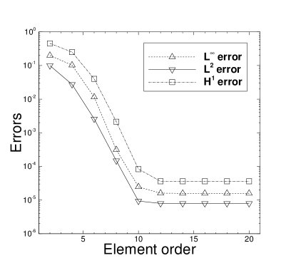
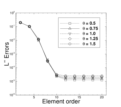
(a) (b)

Figure 1: Spatial convergence tests: (a) $L^{\infty}$, $L^{2}$ and $H^{1}$ errors as a function of the element order (fixed $\Delta t=0.001$, $t_{0}=0.1$ and $t_{f}=0.2$) computed using the algorithm with $\theta=0.75$. (b) $L^{\infty}$ errors as a function of the element order computed using algorithms corresponding to several $\theta$ values.

parameter	value	parameter	value
$C_{0}$	$0$	$\lambda$	$0.01$
$m$	$0.01$	$\eta$	$0.1$
$\theta$	$1/2\sim 3/2$	$\Delta t$	(varied)
$\Delta t_{\min}$	$1e-4$	$S$	$\sqrt{\frac{4\gamma_{0}\lambda\omega_{0}}{m\Delta t}}$ or $\sqrt{\frac{4\gamma_{0}\lambda\omega_{0}}{m\Delta t_{\min}}}$
$t_{0}$	$0.1$	$t_{f}$	$0.2$ (spatial tests) or $0.3$ (temporal tests)
Element order	(varied)	Elements	$2$

Table 2: Simulation parameter values for convergence tests.

We discretize the domain using two equal-sized quadrilateral elements, with the element order and the time step size $\Delta t$ varied systematically in the spatial and temporal convergence tests. The algorithm from Section 2 is employed to numerically integrate the Cahn-Hilliard equation in time from $t=t_{0}$ to $t=t_{f}$. The initial phase field function $\phi_{in}$ is obtained by setting $t=t_{0}$ in the analytic expression (51). The numerical solution at $t=t_{f}$ is then compared with the analytic solution, and various norms of the errors are computed. The values for the simulation parameters are summarized in Table 2 for this problem.

To test the spatial convergence rate, we employ a fixed $\Delta t=0.001$, $t_{0}=0.1$ and $t_{f}=0.2$, and vary the element order systematically between $2$ and $20$. Then for each element order, the numerical errors of $\phi$ in $L^{\infty}$, $L^{2}$ and $H^{1}$ norms at $t=t_{f}$ are obtained. Figure 1(a) shows these errors as a function of the element order using the algorithm with $\theta=3/4$. We observe an exponential decrease of the numerical errors with increasing element order (for element orders $10$ and below), and a level-off of the error curves beyond element order $12$ due to the saturation of temporal errors. Figure 1(b) shows the $L^{\infty}$ errors versus the element order obtained using the algorithms corresponding several $\theta$ values ranging from $1/2$ to $3/2$. Some differences in the saturation error level (for orders $12$ and above) can be observed with different algoirthms. The saturation error appears larger for algorithms with larger $\theta$ values.

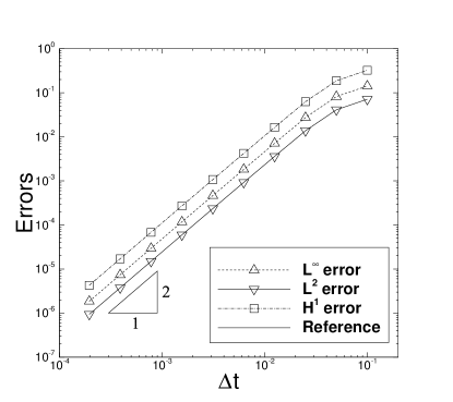
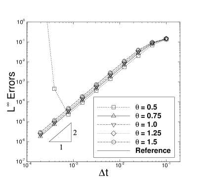
(a) (b)

Figure 2: Temporal convergence tests: (a) $L^{\infty}$, $L^{2}$ and $H^{1}$ errors as a function of time step size $\Delta t$ (fixed element order $16$, $t_{0}=0.1$ and $t_{f}=0.3$) computed using the algorithm corresponding to $\theta=0.75$. (b) $L^{\infty}$ errors as a function of $\Delta t$ computed using the algorithms corresponding to several $\theta$ values.

To test the temporal convergence rate, we employ a fixed element order $16$, $t_{0}=0.1$ and $t_{f}=0.3$, and vary the time step size $\Delta t$ systematically between $0.1$ and $1.953125\times 10^{-4}$. For each $\Delta t$ the numerical errors in different norms are computed at $t=t_{f}$. Figure 2(a) shows the numerical errors as a function of $\Delta t$ obtained using the algorithm with $\theta=3/4$. A second-order convergence rate is observed. Figure 2(b) shows the $L^{\infty}$ errors versus $\Delta t$ obtained using the algorithms corresponding to several $\theta$ values. The errors are generally smaller with a smaller $\theta$ value in the algorithm. However, with $\theta=1/2$ (the lower boundary for the $\theta$ range, corresponding to the Crank-Nicolson scheme) we observe a weak instability when $\Delta t$ becomes small (below $\Delta t=0.00078125$), which results in larger errors with the two smallest $\Delta t$ values in the test. Note that $t_{f}$ is fixed in the tests, and a larger number of time steps are computed with a smaller $\Delta t$. The observation of poor performance of the algorithm with $\theta=1/2$ will appear again with further numerical tests in subsequent sections.

The test results of this section indicate that the family of algorithms presented in Section 2 exhibits a spatial exponential convergence rate and a temporal second-order convergence rate.

3.2 Evolution and Coalescence of Drops

In this section we consider the evolution of a drop and the coalescence of two drops to illustrate the dynamics of the Cahn-Hilliard equation and the energy stability of the family of algorithms from Section 2.

Evolution of a Drop

We first look into the evolution of a material drop under the Cahn-Hilliard dynamics. Consider a square domain $\Omega=\{\ (x,y)\ |\ 0\leqslant x,y\leqslant 1\ \},$ and two materials contained in this domain. It is assumed that the evolution of the material regions is described by the Cahn-Hilliard equation, and that $\phi=1$ and $-1$ correspond to the bulk of the first and second materials, respectively. At $t=0$, the first material is located in a smaller square region with dimension $2h_{0}\times 2h_{0}$ (where $h_{0}=0.2$) around the center of the domain, and the second material fills the rest of the domain. The goal here is to study the evolution dynamics of these material regions.

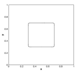
(a) $t=0.001$

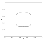
(b) $t=1$

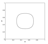
(c) $t=4$

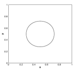
(d) $t=10$

Figure 3: Temporal sequence of snapshots showing the evolution of a drop visualized by the contour level $\phi=0$. Results are obtained with the algorithm $\theta=0.75$, and time step size $\Delta t=10^{-3}$.

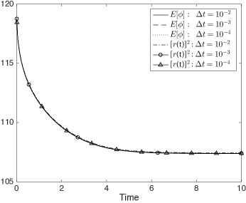
Figure 4: Time histories of $E[\phi]$ and $[r(t)]^{2}$ computed using several $\Delta t$ values, with the algorithm $\theta=0.75$.

We employ the algorithms from Section 2 to numerically solve the Cahn-Hilliard equation with $g(\mathbf{x},t)=0$ in this domain. We discretize the domain using $400$ quadrilateral elements, with $20$ equal-sized elements along both $x$ and $y$ directions. The boundary conditions (2a) and (2b), with $g_{a}=0$ and $g_{b}=0$, are imposed on the domain boundaries. The initial distribution of the materials is given by

$$\phi_{in}(\mathbf{x})=\frac{1}{2}\left[\tanh\frac{x-x_{0}+h_{0}}{\sqrt{2}\eta}-\tanh\frac{x-x_{0}-h_{0}}{\sqrt{2}\eta}\right]\cdot\frac{1}{2}\left[\tanh\frac{y-y_{0}+h_{0}}{\sqrt{2}\eta}-\tanh\frac{y-y_{0}-h_{0}}{\sqrt{2}\eta}\right],$$ (52)

where $(x_{0},y_{0})=(0.5,0.5)$ is the center of the domain. We employ the following (non-dimensional) parameter values for this problem:

$$\left\{\begin{split}&\eta=0.01,\quad\sigma=151.15,\quad C_{0}=0,\\ &\lambda=\frac{3}{2\sqrt{2}}\sigma\eta,\quad m=\frac{10^{-6}}{\lambda},\quad S=\sqrt{\frac{4\gamma_{0}\lambda\omega_{0}}{m\Delta t}},\\ &\text{element order:}\ 8,\quad\text{number of elements:}\ 400,\\ &\Delta t\ \text{varied},\quad\theta\ \text{varied}.\end{split}\right.$$ (53)

Figure 3 shows the evolution of the material regions with a temporal sequence of snapshots of the interface (visualized by the contour level $\phi=0$) between the two materials. These results are computed with a time step size $\Delta t=0.001$ using the algorithm corresponding to $\theta=0.75$. The initially square region of the first material evolves gradually into a circular region under the Cahn-Hilliard dynamics. Figure 4 shows the time histories of the potential energy $E[\phi]$ defined in (5) and the quantity $[r(t)]^{2}$ computed from equation (7), obtained using time step sizes $\Delta t=10^{-4}$, $10^{-3}$ and $10^{-2}$ with the algorithm $\theta=0.75$. Both $E[\phi]$ and $[r(t)]^{2}$ decrease over time, and they gradually level off at a certain level. In particular, we observe that the history curves for $E[\phi]$ and $[r(t)]^{2}$ essentially overlap with one another, which is consistent with the fact that $r(t)$ computed based on equation (7) is an approximation of $\sqrt{E[\phi]}$ (see equation (6)).

(a) $t=10^{4}$

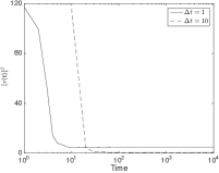
Figure 5: Drop evolution computed using large $\Delta t$ values: (a) Drop configuration at $t=10^{4}$ computed using $\Delta t=10$; (b)-(c) Time histories of $E[{\phi}]$ and $[r(t)]^{2}$ obtained with $\Delta t=1,10.$ Simulation results are obtained with the algorithm $\theta=1$ (BDF2).

The energy stable nature of the current algorithms allows the use of large or fairly large time step sizes in the computations. This is demonstrated by the results in Figure 5. Figure 5(a) shows the interface between the two materials at a much later time $t=10^{4}$, computed using a large time step size $\Delta t=10$ with the algorithm $\theta=1$. Figures 5(b) and (c) show the time histories of $E[\phi]$ and $[r(t)]^{2}$ corresponding to two large time step sizes $\Delta t=1$ and $\Delta t=10$ with the algorithm $\theta=1$. The long time histories demonstrate that the computations with these large $\Delta t$ values are indeed stable using the current algorithm. On the other hand, because these time step sizes are very large, we do not expect that the computation results will be accurate with these $\Delta t$ values. It is observed that the $E[\phi]$ and $[r(t)]^{2}$ values in Figures 5(b)-(c) are quite different from those obtained with small $\Delta t$ (see Figure 4). In particular, we observe that $[r(t)]^{2}$ decreases sharply at the beginning, and for a given $\Delta t$ its history curve gradually levels off at a certain value over time. With a larger $\Delta t$, the $[r(t)]^{2}$ history tends to level off at a smaller value. With very large $\Delta t$ values, $[r(t)]^{2}$ will essentially tend to zero. This seems to be a common characteristic to the family of algorithms developed in this work.

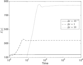
(a) $E{[}\phi{]}$ with $\theta=0.75$

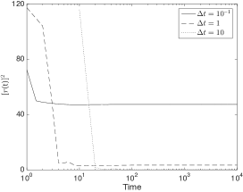
(b) ${[}r(t){]}^{2}$ with $\theta=0.75$

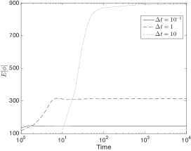
(c) $E{[}\phi{]}$ with $\theta=1.25$

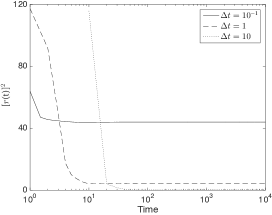
(d) ${[}r(t){]}^{2}$ with $\theta=1.25$

Figure 6: Time histories of $E[\phi]$ and $[r(t)]^{2}$ corresponding to several large $\Delta t$ values obtained with the algorithms $\theta=0.75$ and $\theta=1.25$.

Similar behaviors have been observed with the other members of this family of algorithms for large $\Delta t$ values. This is demonstrated by Figure 6, in which we show time histories of $E[\phi]$ and $[r(t)]^{2}$ corresponding to three time step sizes $\Delta t=0.1$, $1$ and $10$, computed using the algorithms $\theta=0.75$ and $\theta=1.25$. The long-time histories signify the stability of these computations.

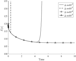
(a) $\theta=0.5$

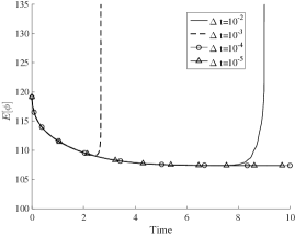
(b) $\theta=1.5$

Figure 7: Time histories of $E[\phi]$ computed with the algorithms $\theta=0.5$ (a) and $\theta=1.5$ (b), using various $\Delta t$ values.

Among the family of algorithms ($\frac{1}{2}\leqslant\theta\leqslant\frac{3}{2}$) presented in Section 2, we observe from numerical simulations that the two members on the borders, $\theta=\frac{1}{2}$ and $\theta=\frac{3}{2}$, seem to have a performance inferior to the rest of this family. Figure 7 shows the time histories of $E[\phi]$ corresponding to several $\Delta t$ values, ranging from $10^{-2}$ to $10^{-5}$, computed using the algorithms $\theta=\frac{1}{2}$ and $\theta=\frac{3}{2}$. We observe that the computation using the algorithm $\theta=\frac{1}{2}$ becomes unstable with $\Delta t=10^{-2}$, $10^{-3}$ and $10^{-4}$, and the computation using $\theta=\frac{3}{2}$ becomes unstable with $\Delta t=10^{-2}$ and $10^{-3}$. We do not observe such an instability with the other members of this family of algorithms. Note that the Theorem 2.1 ensures the energy stability of the semi-discretized algorithm (discrete in time, continuous in space) given by (13a)–(13e) for $\theta=\frac{1}{2}$ and $\theta=\frac{3}{2}$. It is possible that the fully discretized algorithm (in both space and time) may not preserve this energy stability, which is likely why we observe this instability with the algorithms $\theta=\frac{1}{2}$ and $\theta=\frac{3}{2}$.

Coalescence of Two Drops

We next consider the coalescence of two material drops governed by the Cahn-Hilliard equation. The computational domain and the setting follow those for the single-drop case discussed above. The difference lies in the initial distribution of the materials. Here we assume that at $t=0$ the first material occupies two circular regions that are right next to each other and the second material fills the rest of the domain. The two regions of the first material then coalesce with each other to form a single drop under the Cahn-Hilliard dynamics. The goal is to illustrate this process using the current algorithms.

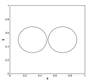
(a) $t=3\times 10^{-3}$

(b) $t=0.25$

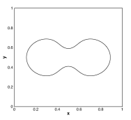
(c) $t=2$

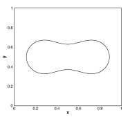
(d) $t=8$

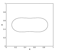
(e) $t=20$

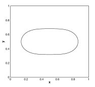
(f) $t=40$

(g) $t=70$

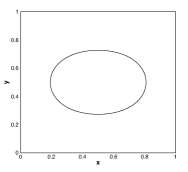
(h) $t=100$

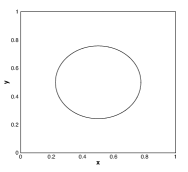
(i) $t=200$

Figure 8: Temporal sequence of snapshots showing the coalescence of two circular drops. Results are obtained with the algorithm $\theta=0.75$.

More specifically, we employ the following initial distribution for the materials

$$\phi_{in}(\bm{x})=1-\tanh\frac{|\bm{x}-\bm{x}_{0}|-R_{0}}{\sqrt{2}\eta}-\tanh\frac{|\bm{x}-\bm{x}_{1}|-R_{0}}{\sqrt{2}\eta},$$ (54)

where $\bm{x}_{0}=(x_{0},y_{0})=(0.3,0.5)$ and $\bm{x}_{1}=(x_{1},y_{1})=(0.7,0.5)$ are the centers of the circular regions for the first material, and $R_{0}=0.19$ is the radius of these circles. In the Cahn-Hilliard equation (1) we set $g=0$. The boundary conditions (2a) and (2b) with $g_{a}=0$ and $g_{b}=0$ are imposed on the domain boundaries. The other simulation parameters follow those given in (53).

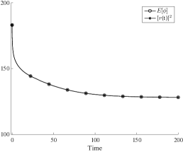
(a) $\theta=0.75$

(b) $\theta=1.25$

Figure 9: Time histories of $E[\phi]$ and $[r(t)]^{2}$ for the coalescence of two drops, computed using the algorithm (a) $\theta=0.75$, and (b) $\theta=1.25$.

The process of coalescence of the two drops is demonstrated in Figure 8 with a temporal sequence of snapshots of the interfaces between the materials (visualized by the contour level $\phi=0$). These results are computed using the algorithm $\theta=0.75$, with a time step size $\Delta t=0.001$. Figure 9 shows the time histories of $E[\phi]$ and $[r(t)]^{2}$ computed using the algorithms corresponding to $\theta=0.75$ and $\theta=1.25$. The general characteristics for these history signals are similar to those for the case with a single drop. Both $E[\phi]$ and $[r(t)]^{2}$ are observed to decrease over time, and their history curves overalp with each other.

3.3 Spinodal Decomposition

In this section we consider the spinodal decomposition of a homogeneous mixture into two coexisting phases governed by the Cahn-Hilliard equation as another test of the algorithms developed herein.

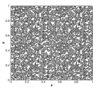
(a) $t=0$

(b) $t=0.1$

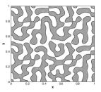
(c) $t=0.2$

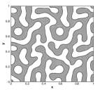
(d) $t=0.5$

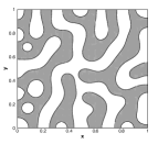
(e) $t=2$

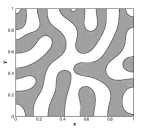
(f) $t=4$

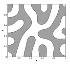
(g) $t=7$

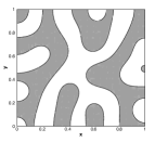
(h) $t=10$

Figure 10: Spinodal decomposition: temporal sequence of snapshots of the interfaces visualized by $\phi=0$. Simulation results are obtained using the algorithm $\theta=1.25$.

Consider the domain $\Omega=\{\ (x,y)\ |\ 0\leqslant x,y\leqslant 1\ \}$, and a homogeneous mixture of two materials with a random initial distribution (see Figure 10(a)). The evolution of the materials is assumed be described by the Cahn-Hilliard equation (1) with $g(\mathbf{x},t)=0$, and the goal is to simulate this evolution process.

We simulate this problem using the algorithms from Section 2. The domain is discretized using $400$ quadrilateral elements, with $20$ uniform elements along both $x$ and $y$ directions. The boundary conditions (2a) and (2b) with $g_{a}=0$ and $g_{b}=0$ are imposed on the domain boundaries. The initial random distribution of $\phi_{in}(\mathbf{x})$ is generated using a random number generator from the standard library of C language (see Figure 10(a)). The following simulation parameter values are employed for this problem:

$$\left\{\begin{split}&\eta=0.01,\quad\lambda=0.001,\quad m=0.001,\\ &C_{0}=0,\quad\Delta t=0.001,\quad S=\sqrt{\frac{4\gamma_{0}\lambda\omega_{0}}{m\Delta t}},\\ &\text{element order:}\ 8,\quad\text{number of elements:}\ 400,\\ &\theta=\ 0.75,\ 1.0,\ 1.25.\end{split}\right.$$ (55)

Figure 10 shows the typical evolution process of the mixture with a temporal sequence of snapshots of the interfaces formed between the two phases. The interface is visualized by the contour level $\phi(\mathbf{x},t)=0$. The lighter regions represents the first phase and the darker region represents the second phase. These results are obtained using the algorithm $\theta=1.25$. It can be observed that two phases emerge from the initially homogeneous distribution of the mixture. Over time the grains of the two phases become increasingly coarser, and a certain pattern can be observed from the two regions.

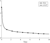
(a) $\theta=0.75$

(b) $\theta=1$

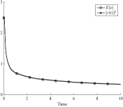
(c) $\theta=1.25$

Figure 11: Time histories of $E[\phi]$ and $[r(t)]^{2}$ for spinodal decomposition obtained with several algorithms corresponding to (a) $\theta=0.75,$ (b) $\theta=1,$ (c) $\theta=1.25.$

Figure 11 shows the time histories of the potential free energy $E[\phi]$ and the variable $[r(t)]^{2}$ of the system obtained using three algorithms, corresponding to $\theta=0.75$, $\theta=1$ and $\theta=1.25$. We note that the history curves for $E[\phi]$ and $[r(t)]^{2}$ essentially overlap with each other, and that the results obtained with different algorithms agree well with one another.

3.4 Two-Phase Flow: Rising Air Bubble in Water

As another test case, in this section we demonstrate the performance of the algorithm developed herein in the context of a two-phase flow solver, and simulate the two-phase flow of an air bubble rising through the water.

Following DongS2012 ; Dong2012 , we consider a system consisting of two immiscible incompressible fluids, and combine the Cahn-Hilliard equation and the incompressible Navier-Stokes equations with variable density and variable viscosity to model such a system; see DongS2012 ; DongW2016 for details. We then combine the family of algorithms presented in Section 2 for the Cahn-Hilliard equation and the algorithm from DongS2012 for the momentum equations to form an overall method for numerically solving the coupled system of Cahn-Hilliard and Navier-Stokes equations. Note that the algorithm for the momentum equation employed here is a semi-implicit type scheme and is only conditionally stable DongS2012 . So the overall algorithm for the two-phase flows is not energy stable.

Density [$kg/m^{3}$]:	air - $\rho_{1}=1.204$	water - $\rho_{2}=998.207$
Dynamic viscosity [$kg/(m\cdot s)$]:	air - $\mu_{1}=1.78\times 10^{-5}$	water - $\mu_{2}=1.002\times 10^{-3}$
Surface tension [$kg/s^{2}$]:	air/water - $\sigma=7.28\times 10^{-2}$
Gravity [$m/s^{2}$]:	$g_{r}=9.8$

Table 3: Physical property values of air and water.

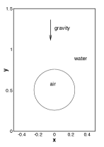
(a) $t=0.05$

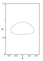
(b) $t=0.4$

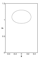
(c) $t=0.8$

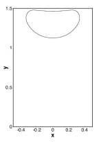
(d) $t=1.15$

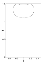
(e) $t=1.4$

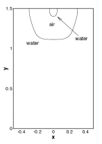
(f) $t=1.45$

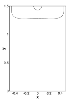
(g) $t=1.7$

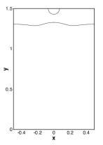
(h) $t=2.05$

Figure 12: Time sequence of snapshots of an air bubble (initially circular) rising in water within a solid container, showing the bubble breakup on the upper wall and the formation of an air cavity.

We consider a solid container occupying the domain $-\frac{L}{2}\leqslant x\leqslant\frac{L}{2}$ and $0\leqslant y\leqslant\frac{3}{2}L$, where $L=1cm$ (see Figure 12(a)). The container is filled with water, and an air bubble is trapped inside the water. The air bubble is initially circular with a diameter $2R_{0}=0.5L=0.5cm$ and its center located at $\mathbf{x}_{0}=(x_{0},y_{0})=(0,0.5L)$, and it is held at rest. The container walls are assumed to have a neutral wettability ($90$-degree contact-angle), and the gravity is assumed to point downward. At $t=0$, the air bubble is released, and starts to rise through the water due to buoyancy. The bubble eventually breaks up on the upper wall and forms an air cavity at the top of the container. The goal is to simulate this process.

The physical parameters for the air and water are summarized in Table 3. We choose $L$ as the characteristic length scale, the air density as the characteristic density scale $\varrho_{0}$, and $U_{0}=\sqrt{g_{r0}L}$ ($g_{r0}=1m/s^{2}$) as the characteristic velocity scale. All the physical parameters are then normalized according to Table 1.

In the simulations the domain is discretized using $600$ quadrilateral elements, with $20$ and $30$ uniform elements in $x$ and $y$ directions, respectively. An element order $8$ is employed in the simulations. We impose the boundary conditions (2a) and (2b) with $g_{a}=0$ and $g_{b}=0$ for the phase field function $\phi$ and the no-slip condition for the velocity on the container walls. The initial velocity is assumed to be zero, and the initial distribution of the phase field function is given by

$$\phi_{in}(\bm{x})=-\tanh\frac{|\bm{x}-\bm{x}_{0}|-R_{0}}{\sqrt{2}\eta}.$$ (56)

The values for the simulation parameters in this problem are given by

$$\left\{\begin{split}&\frac{\eta}{L}=0.01,\quad\frac{\sigma}{\varrho_{0}U_{0}^{2}L}=604.6\ (\text{surface tension}),\quad\lambda=\frac{3}{2\sqrt{2}}\sigma\eta,\quad\frac{m}{L/(\varrho_{0}U_{0})}=\frac{10^{-7}}{\lambda/(\varrho_{0}U_{0}^{2}L^{2})},\\ &C_{0}=0,\quad\frac{\Delta t}{L/U_{0}}=2.5e-5,\quad S=\sqrt{\frac{4\gamma_{0}\lambda\omega_{0}}{m\Delta t}},\\ &\text{element order:}\ 8,\quad\text{number of elements:}\ 600,\\ &\theta=0.75.\end{split}\right.$$ (57)

The dynamics of this two-phase flow is illustrated by Figure 12, in which we have shown a temporal sequence of snapshots of the air-water interface in this system. The interface is visualized by the contour level $\phi(\mathbf{x},t)=0$. As the system is released the air bubble rises through the water and experiences significant deformations (Figure 12(b)-(d)). The bubble exhibits the typical shape of a circular “cap” (Figure 12(b)) when it is still far away from the upper wall. But as the bubble approaches the upper wall, its shape is affected by the presence of the wall significantly (Figures 12(c)-(d)). After the bubble touches the upper wall, it traps a layer of water between the wall and its upper side (Figure 12(e)). The trapped water becomes a water drop sitting on the upper wall over time (Figure 12(g)). The interface formed between the bulk of air and the bulk of water moves sideways on the wall, and the air forms a cavity at the top of the container (Figures 12(f)-(h)). Our method has captured this process and the interaction between the air-water interface and the wall.

4 Concluding Remarks

In this paper we have developed a family of second-order energy-stable schemes for the Cahn-Hilliard type equations. We start with the reformulated system of equations based on the scalar auxiliary variable approach, and approximate this system at time step $(n+\theta)$, and then develop corresponding numerical approximations that are second-order accurate and unconditionally energy stable. This family of approximations contains the often-used Crank-Nicolson scheme and the second-order backward differentiation formula as particular cases. We have also developed an efficient solution algorithm to overcome the difficulty caused by the unknown scalar auxiliary variable in the discrete system of equations resulting from this family of schemes. Our overall computation algorithm only requires the solution of four de-coupled individual Helmholtz type equations within each time step, and these equations only involve constant and time-independent coefficient matrices that can be pre-computed.

While the current paper is only concerned with the numerical approximation of the Cahn-Hilliard equation, the family of second-order energy-stable approximations is readily applicable to other types of equations resulting from gradient flows. When combined with the invariant energy quadratization or scalar auxiliary variable approach, they can be readily used to design energy-stable schemes for other gradient flows.

Appendix A: Proof of Theorem 2.1

We note first the following useful relation ($\chi$ denoting a generic scalar variable):

$$\left(\chi^{n+1}-2\chi^{n}+\chi^{n-1}\right)\left[\left(\theta+\frac{1}{2}\right)\chi^{n+1}-2\theta\chi^{n}+\left(\theta-\frac{1}{2}\right)\chi^{n-1}\right]\\ =\theta\left|\chi^{n+1}-2\chi^{n}+\chi^{n-1}\right|^{2}+\frac{1}{2}\left(\left|\chi^{n+1}-\chi^{n}\right|^{2}-\left|\chi^{n}-\chi^{n-1}\right|^{2}\right),$$ (58)

$$\begin{split}&\chi^{n+\theta}\left[\left(\theta+\frac{1}{2}\right)\chi^{n+1}-2\theta\chi^{n}+\left(\theta-\frac{1}{2}\right)\chi^{n-1}\right]\\ &\quad=\frac{1}{2}\theta\left(\theta-\frac{1}{2}\right)(3-2\theta)\left|\chi^{n+1}-2\chi^{n}+\chi^{n-1}\right|^{2}+\frac{1}{2}\left(\frac{3}{2}-\theta\right)\left(\left|\chi^{n+1}\right|^{2}-\left|\chi^{n}\right|^{2}\right)\\ &\qquad+\frac{1}{2}\left(\theta-\frac{1}{2}\right)\left(\left|2\chi^{n+1}-\chi^{n}\right|^{2}-\left|2\chi^{n}-\chi^{n-1}\right|^{2}\right),\end{split}$$ (59)

This relation can be verified by elementary operations.

Assume that $g=0$, $g_{a}=0$, and $g_{b}=0$. Multiply $\Delta t\mathscr{H}^{n+\theta}$ to equation (13a) and integrate over $\Omega$, and we have

$$\int_{\Omega}\left[\left(\theta+\frac{1}{2}\right)\phi^{n+1}-2\theta\phi^{n}+\left(\theta-\frac{1}{2}\right)\phi^{n-1}\right]\mathscr{H}^{n+\theta}=m\Delta t\int_{\Omega}\mathscr{H}^{n+\theta}\nabla^{2}\mathscr{H}^{n+\theta}.$$ (60)

Multiplying $\Delta t\left.\frac{\partial\phi}{\partial t}\right|^{n+\theta}$ to equation (13b) and integrating over $\Omega$ leads to

$$\begin{split}&\int_{\Omega}\mathscr{H}^{n+\theta}\left[\left(\theta+\frac{1}{2}\right)\phi^{n+1}-2\theta\phi^{n}+\left(\theta-\frac{1}{2}\right)\phi^{n-1}\right]\\ &=-\lambda\int_{\Omega}\nabla^{2}\phi^{n+\theta}\left[\left(\theta+\frac{1}{2}\right)\phi^{n+1}-2\theta\phi^{n}+\left(\theta-\frac{1}{2}\right)\phi^{n-1}\right]\\ &\quad+S\int_{\Omega}\left(\phi^{n+1}-2\phi^{n}+\phi^{n-1}\right)\left[\left(\theta+\frac{1}{2}\right)\phi^{n+1}-2\theta\phi^{n}+\left(\theta-\frac{1}{2}\right)\phi^{n-1}\right]\\ &\quad+\frac{r^{n+\theta}}{\sqrt{E[\bar{\phi}^{n+\theta}]}}\int_{\Omega}h(\bar{\phi}^{n+\theta})\left[\left(\theta+\frac{1}{2}\right)\phi^{n+1}-2\theta\phi^{n}+\left(\theta-\frac{1}{2}\right)\phi^{n-1}\right].\end{split}$$ (61)

Multiplying $2r^{n+\theta}\Delta t$ to equation (13c) leads to

$$2r^{n+\theta}\left[\left(\theta+\frac{1}{2}\right)r^{n+1}-2\theta r^{n}+\left(\theta-\frac{1}{2}\right)r^{n-1}\right]\\ =\frac{r^{n+\theta}}{\sqrt{E[\bar{\phi}^{n+\theta}]}}\int_{\Omega}h(\bar{\phi}^{n+\theta})\left[\left(\theta+\frac{1}{2}\right)\phi^{n+1}-2\theta\phi^{n}+\left(\theta-\frac{1}{2}\right)\phi^{n-1}\right].$$ (62)

Summing up equations (60) and (62), and then subtracting equation (61), results in

$$\begin{split}&2r^{n+\theta}\left[\left(\theta+\frac{1}{2}\right)r^{n+1}-2\theta r^{n}+\left(\theta-\frac{1}{2}\right)r^{n-1}\right]\\ &=-m\Delta t\int_{\Omega}\nabla\mathscr{H}^{n+\theta}\cdot\nabla\mathscr{H}^{n+\theta}-\lambda\int_{\Omega}\nabla\phi^{n+\theta}\cdot\left[\left(\theta+\frac{1}{2}\right)\nabla\phi^{n+1}-2\theta\nabla\phi^{n}+\left(\theta-\frac{1}{2}\right)\nabla\phi^{n-1}\right]\\ &\quad-S\int_{\Omega}\left(\phi^{n+1}-2\phi^{n}+\phi^{n-1}\right)\left[\left(\theta+\frac{1}{2}\right)\phi^{n+1}-2\theta\phi^{n}+\left(\theta-\frac{1}{2}\right)\phi^{n-1}\right]\end{split}$$ (63)

where we have performed integration by part on the right-hand-side (RHS) of equation (60) and the first term on the RHS of equation (61), and used equations (13b), (13d) and (13e).

Use the relations (58) and (12) to transform the corresponding terms in (63), and then collect related terms, and one would arrive at the discrete energy balance equation (14).

Appendix B. Proof of Theorem 2.3

Substituting $\psi_{2}^{n+1}$ from (36a) into equations (35a) and (35b) leads to

$$\nabla^{2}\left(\nabla^{2}\phi_{2}^{n+1}\right)-\frac{S}{\lambda\omega_{0}}\nabla^{2}\phi_{2}^{n+1}+\frac{\gamma_{0}}{\lambda\omega_{0}m\Delta t}\phi_{2}^{n+1}=\frac{1}{2\lambda}\nabla^{2}b^{n},$$ (64a)

$$\mathbf{n}\cdot\nabla\left(\nabla^{2}\phi_{2}^{n+1}\right)=\frac{1}{2\lambda}\mathbf{n}\cdot\nabla b^{n},\quad\text{on}\ \partial\Omega,$$ (64b)

where we have used equation (36b) and the relation $\alpha\left(\alpha+\frac{S}{\lambda\omega_{0}}\right)=-\frac{\gamma_{0}}{\lambda\omega_{0}m\Delta t}$. The system of equations (64a), (64b) and (36b) is equivalent to the system consisting of equations (35a)–(36b). By integrating equation (64a) over the domain $\Omega$, we conclude that $\phi_{2}^{n+1}$ has the property

$$\int_{\Omega}\phi_{2}^{n+1}=0,$$ (65)

where we have used the divergence theorem and the equations (64b) and (36b).

Define function $\xi(\mathbf{x})$ by

$$\left\{\begin{split}&\nabla^{2}\xi=\phi_{2}^{n+1},\\ &\mathbf{n}\cdot\nabla\xi=0,\quad\text{on}\ \partial\Omega,\\ &\int_{\Omega}\xi=\frac{\omega_{0}m\Delta t}{2\gamma_{0}}\int_{\Omega}b^{n}.\end{split}\right.$$ (66)

Let

$$\Phi=\nabla^{2}\phi_{2}^{n+1}-\frac{S}{\lambda\omega_{0}}\phi_{2}^{n+1}+\frac{\gamma_{0}}{\lambda\omega_{0}m\Delta t}\xi-\frac{1}{2\lambda}b^{n}.$$ (67)

Then equations (64a), (64b) and (65) are transformed into

$$\nabla^{2}\Phi=0,$$ (68a)

$$\mathbf{n}\cdot\nabla\Phi=0,\quad\text{on}\ \partial\Omega,$$ (68b)

$$\int_{\Omega}\Phi=0,$$ (68c)

where we have used (66) and (36b). So we conclude that $\Phi=0$ and

$$\nabla^{2}\phi_{2}^{n+1}-\frac{S}{\lambda\omega_{0}}\phi_{2}^{n+1}+\frac{\gamma_{0}}{\lambda\omega_{0}m\Delta t}\xi=\frac{1}{2\lambda}b^{n}.$$ (69)

Taking the $L^{2}$ inner product between this equation and $\phi_{2}^{n+1}$ and integrating by part, we get

$$\frac{1}{2\lambda}\int_{\Omega}b^{n}\phi_{2}^{n+1}=-\int_{\Omega}\left|\nabla\phi_{2}^{n+1}\right|^{2}-\frac{S}{\lambda\omega_{0}}\int_{\Omega}\left|\phi_{2}^{n+1}\right|^{2}-\frac{\gamma_{0}}{\lambda\omega_{0}m\Delta t}\int_{\Omega}\left|\nabla\xi\right|^{2}\leqslant 0,$$ (70)

where we have used the divergence theorem and equation (66).

References

• [1] H. Abels, H. Garcke, and G. Grün. Thermodynamically consistent, frame indifferent diffuse interface models for incompressible two-phase flows with different densities. Mathematical Models and Methods in Applied Sciences, 22:1150013, 2012.
• [2] D.M. Anderson, G.B. McFadden, and A.A. Wheeler. Diffuse-interface methods in fluid mechanics. Annual Review of Fluid Mechanics, 30:139–165, 1998.
• [3] V.E. Badalassi, H.D. Ceniceros, and S. Banerjee. Computation of multiphase systems with phase field models. Journal of Computal Physics, 190:371–397, 2003.
• [4] S. Badia, F. Guillen-Gonzalez, and J.V. Gutierrez-Santacreu. Finite element approximation of nematic liquid crystal flows using a saddle-point structure. Journal of Computational Physics, 230:1686–1706, 2011.
• [5] J.W. Cahn and J.E. Hilliard. Free energy of a nonuniform system. I interfacial free energy. Journal of Chemical Physics, 28:258–267, 1958.
• [6] S. Dong. On imposing dynamic contact-angle boundary conditions for wall-bounded liquid-gas flows. Computer Methods in Applied Mechanics and Engineering, 247–248:179–200, 2012.
• [7] S. Dong. An efficient algorithm for incompressible N-phase flows. Journal of Computational Physics, 276:691–728, 2014.
• [8] S. Dong. An outflow boundary condition and algorithm for incompressible two-phase flows with phase field approach. Journal of Computational Physics, 266:47–73, 2014.
• [9] S. Dong. Wall-bounded multiphase flows of N immiscible incompressible fluids: consistency and contact-angle boundary condition. Journal of Computational Physics, 338:21–67, 2017.
• [10] S. Dong. Multiphase flows of N immiscible incompressible fluids: a reduction-consistent and thermodynamically-consistent formulation and associated algorithm. Journal of Computational Physics, 361:1–49, 2018.
• [11] S. Dong and J. Shen. A time-stepping scheme involving constant coefficient matrices for phase field simulations of two-phase incompressible flows with large density ratios. Journal of Computational Physics, 231:5788–5804, 2012.
• [12] S. Dong and X. Wang. A rotational pressure-correction scheme for incompressible two-phase flows with open boundaries. PLOS One, 11(5):e0154565, 2016.
• [13] C.M. Elliot, D.A. French, and F.A. Milner. A second order splitting method for the cahn-hilliard equation. Numerische Mathematik, 54:575–590, 1989.
• [14] C.M. Elliot and A.M. Stuart. The global dynamics of discrete semilinear parabolic equations. SIAM Journal on Numerical Analysis, 30:1622–1663, 1993.
• [15] J.D. Eyre. An unconditionally stable one-step scheme for gardient system. unpublished. www.math.utah.edu/~eyre/research/methods/stable.ps.
• [16] X. Feng. Fully discrete finite element approximations of the navier-stokes-cahn-hilliard diffuse interface model for two-phase fluid flows. SIAM Journal on Numerical Analysis, 44:1049–1072, 2006.
• [17] X. Feng and A. Prohl. Error analysis of a mixed finite element method for the cahn-hilliard equation. Numerische Mathematik, 99:47–84, 2004.
• [18] D. Furihata. A stable and conservative finite difference scheme for the cahn-hilliard equation. Numerische Mathematik, 87:675–699, 2001.
• [19] H. Gomez and T.J.R. Hughes. Provably unconditionally stable, second-order time accurate, mixed variational methods for phase-field models. Journal of Computational Physics, 230:5310–5327, 2011.
• [20] F. Guillen-Gonzalez and G. Tierra. On linear schemes for a cahn-hilliard diffuse interface model. Journal of Computational Physics, 234:140–171, 2013.
• [21] D. Gurtin, D. Polignone, and J. Vinals. Two-phase binary fluids and immiscible fluids described by an order parameter. Mathematical Models and Methods in Applied Sciences, 6:815–831, 1996.
• [22] P.C. Hohenberg and B.I. Halperin. Theory of dynamic critical phenomena. Review of Modern Physics, 49:435–479, 1977.
• [23] J. Hua, P. Lin, C. Liu, and Q. Wang. Energy law preserving $C^{0}$ finite element schemes for phase field models in two-phase flow computations. Journal of Computal Physics, 230:7115–7131, 2011.
• [24] D. Jacqmin. Calculation of two-phase navier-stokes flows using phase-field modeling. Journal of Computal Physics, 155:96–127, 1999.
• [25] G.E. Karniadakis and S.J. Sherwin. Spectral/hp element methods for computational fluid dynamics, 2nd edn. Oxford University Press, 2005.
• [26] J. Kim, K. Kang, and J. Lowengrub. Conservative multigrid methods for cahn-hilliard fluids. Journal of Computational Physics, 193:511–543, 2004.
• [27] P. Lin, C. Liu, and H. Zhang. An energy law preserving $c^{0}$ finite element scheme for simulating the kinematic effects in liquid crystal dynamics. Journal of Computational Physics, 227:1411–1427, 2007.
• [28] C. Liu and J. Shen. A phase field model for the mixture of two incompressible fluids and its approximation by a fourier-spectral method. Physica D, 179:211–228, 2003.
• [29] J. Lowengrub and L. Truskinovsky. Quasi-incompressible Cahn-Hilliard fluids and topological transitions. Proceedings of Royal Society London A, 454:2617–2654, 1998.
• [30] E.V.L. Mello and O.T.S. Filho. Numerical study of the cahn-hilliard equation in one, two and three dimensions. Physica A, 347:429–443, 2005.
• [31] J. Shen, J. Xu, and J. Yang. The scalar auxiliary variable (sav) approach for gradient flows. Journal of Computational Physics, 353:407–416, 2018.
• [32] J. Shen and X. Yang. A phase-field model and its numerical approximation for two-phase incompressible flows with different densities and viscosities. SIAM Journal on Scientific Computing, 32:1159–1179, 2010.
• [33] G. Tierra and F. Guillen-Gonzalez. Numerical methods for solving the cahn-hilliard equation and its applicability to related energy-based models. Archives of Computational Methods in Engineering, 22:269–289, 2015.
• [34] S.M. Wise. Unconditionally stable finite difference, nonlinear multigrid simulation of the cahn-hilliard-hele-shaw system of equations. Journal of Scientific Computing, 44:1, 2010.
• [35] X. Yang. Linear, first and second-order, unconditionally energy stable numerical schemes for the phase field model of homopolymer blends. Journal of Computational Physics, 327:294–316, 2016.
• [36] P. Yue, J.J. Feng, C. Liu, and J. Shen. A diffuse-interface method for simulating two-phase flows of complex fluids. Journal of Fluid Mechanics, 515:293–317, 2004.
• [37] P. Yue, C. Zhou, and J.J. Feng. Sharp-interface limit of the Cahn-Hilliard model for moving contact lines. J. Fluid Mech., 645:279–294, 2010.
• [38] X. Zheng and S. Dong. An eigen-based high-order expansion basis for structured spectral elements. Journal of Computational Physics, 230:8573–8602, 2011.