False discovery rate control for multiple testing based on p-values with càdlàg distribution functions

Abstract

For multiple testing based on p-values with càdlàg distribution functions, we propose an FDR procedure “BH+” with proven conservativeness. BH+ is at least as powerful as the BH procedure when they are applied to super-uniform p-values. Further, when applied to mid p-values, BH+ is more powerful than it is applied to conventional p-values. An easily verifiable necessary and sufficient condition for this is provided. BH+ is perhaps the first conservative FDR procedure applicable to mid p-values. BH+ is applied to multiple testing based on discrete p-values in a methylation study, an HIV study and a clinical safety study, where it makes considerably more discoveries than the BH procedure.

Keywords: càdlàg distribution functions; false discovery rate; mid p-values.

1 Introduction

Multiple testing aiming at false discovery rate (FDR) control has been routinely conducted in genomics, genetics and drug safety study, where test statistics and their p-values are discrete. The discontinuities in p-value distributions prevent popular FDR procedures, including the BH procedure (“BH”) in Benjamini and Hochberg (1995) and Storey’s procedure in Storey et al. (2004), to exhaust a target FDR bound to reach full power. This has motivated much research in improving existing methods and developing new ones for multiple testing with discrete statistics from three perspectives that are briefly reviewed by Chen et al. (2018). For example, Chen et al. (2018) proposed an estimator of the proportion $\pi_{0}$ of true null hypotheses that is less upwardly biased than that in Storey et al. (2004) and an adaptive BH procedure based on the estimator. However, the improvement of an adaptive procedure may be very small when $\pi_{0}$ is very close to $1$. On the other hand, the procedure in Liang (2016) is for discrete p-values with identical distributions, the BHH procedure of Heyse (2011), even though very powerful, does not have implicit step-up critical constants and is hard to analyze, and the procedures of Döhler et al. (2017) can be more conservative than the BH procedure.

Among all the methods just mentioned, each has been proposed for super-uniform p-values, and none actively utilizes the super-uniformity of discrete p-values or is able to deal with p-value with general distributions. On the other hand, a mid p-value, which was proposed by Lancaster (1961) and whose optimality properties have been studied by Hwang and Yang (2001), is almost surely smaller than conventional p-values. So, a conservative FDR procedure based on mid p-values may be more powerful than one based on conventional p-values, when both are implemented with the same rejection constants. However, mid p-values are sub-uniform (see Definition 1 in Section 2.1), and there does not seem to have been an FDR procedure that is based on mid p-values and whose conservativeness is theoretically proven. This motivates us to investigate FDR procedures that are applicable to p-values with general distributions and effectively utilize the stochastic dominance, if any, of their distributions with respect to the uniform distribution.

In this article, we deal with multiple testing based on p-values whose cumulative distribution functions (CDF’s) are right-continuous with left-limits (i.e., càdlàg). We propose a new FDR procedure, referred to as “BH+”, that is conservative when p-values satisfy the property of “positive regression dependency on subsets of the set of true null hypotheses (PRDS)” and have càdlàg CDF’s. BH+ generalizes BH for multiple testing based on p-values. For multiple testing with discrete, super-uniform p-values under PRDS, BH+ is at least as powerful as BH. Further, BH+ can be applied to mid p-values and is more powerful than BH in this setting. In contrast, BH has not been theoretically proven to be conservative when it is applied to mid p-values. An easy-to-check necessary and sufficient condition is given on when BH+ based on mid p-values rejects at least as many null hypotheses as it does based on conventional p-values. BH+ is perhaps the first conservative FDR procedure that is applicable to sub-uniform p-values, and is implemented by the R package “fdrDiscreteNull” available on CRAN.

The rest of the article is organized as follows. Section 2 discusses two definitions of a two-sided p-value for a discrete statistic and introduces the BH+ procedure. Section 3 contains a simulation study on BH+ when they are applied to p-values of Binomial tests (BT’s) and Fisher’s exact tests (FET’s). Section 4 provides three applications of BH+. The article ends with a discussion in Section 5. All proofs and additional simulation results are relegated into the appendices.

2 Multiple testing with p-values and the BH+ procedure

We will collect in Section 2.1 two definitions of a two-sided p-value and introduce the BH+ procedure in Section 2.2.

2.1 Definitions of a two-sided p-value

For a random variable $X$, let $F$ be its CDF with support $\mathcal{S}$ and probability density function (PDF) $f$. Here $f$ is the Radon-Nikodym derivative $\frac{\mathsf{d}F}{\mathsf{d}\upsilon}$, where $\upsilon$ is the Lebesgue measure or the counting measure on $\mathcal{S}$. For an observation $x_{0}$ from $X$, set

$$l\left(x_{0}\right)=\int_{\left\{x\in\mathcal{S}:f\left(x\right)<f\left(x_{0}\right)\right\}}\mathsf{d}F\left(x\right)\text{ \ and \ }e\left(x_{0}\right)=\int_{\left\{x\in\mathcal{S}:f\left(x\right)=f\left(x_{0}\right)\right\}}\mathsf{d}F\left(x\right).$$

Following Agresti (2002), let $P\left(x_{0}\right)=l\left(x_{0}\right)+e\left(x_{0}\right)$ be the conventional two-sided p-value of $x_{0}$, and following Hwang and Yang (2001), let $Q\left(x_{0}\right)=l\left(x_{0}\right)+2^{-1}e\left(x_{0}\right)$ be the two-sided mid p-value.

Definition 1

A random variable $X$ with range $\left[0,1\right]$ is called “super-uniform” if $\Pr\left(X\leq t\right)\leq t$ for all $t\in\left[0,1\right]$, and it is called “sub-uniform” if $\Pr\left(X\leq t\right)\geq t$ for all $t\in\left[0,1\right]$.

$P$ is super-uniform and $\Pr\left(P\left(X\right)\leq P\left(x\right)\right)=P\left(x\right)$ for all $x\in\mathcal{S}$, whereas $Q$ is sub-uniform and $\Pr\left(Q\left(X\right)\leq Q\left(x\right)\right)=P\left(x\right)$ for all $x\in\mathcal{S}$.

2.2 The BH+ procedure

Consider simultaneously testing $m$ null hypotheses $\left\{H_{i}\right\}_{i=1}^{m}$ based on their associated p-values $\left\{p_{i}\right\}_{i=1}^{m}$ with matching indices. Among $\left\{H_{i}\right\}_{i=1}^{m}$, $m_{0}$ are true and the rest $m_{1}$ false. Let $I_{0}$ be the index set of true null hypotheses, then $m_{0}$ is the cardinality of $I_{0}$ and $\pi_{0}=m_{0}m^{-1}$. For each $i$, let $F_{i}$ be the CDF of $p_{i}$ obtained by assuming $H_{i}$ is a true null, and assume $F_{i}$ has a finite support $S_{i}$. We do not require a p-value to be super-uniform under the null hypothesis but do assume that $F_{i}\left(s\right)=s$ for $s\in S_{i}$ when a $p_{i}$ is super-uniform. Let $\left\{p_{\left(i\right)}\right\}_{i=1}^{m}$ be the order statistics of $\left\{p_{i}\right\}_{i=1}^{m}$ such that $p_{\left(1\right)}\leq p_{\left(2\right)}\leq\cdots\leq p_{\left(m\right)}$. Further, let $H_{\left(i\right)}$ be the null hypothesis associated with $p_{\left(i\right)}$ for each $i$. The BH+ procedure is given by Algorithm 1.

1:Let $F^{\ast}=\max_{1\leq i\leq m}F_{i}$ and denote its support by $S^{\ast}$.

2:At nominal FDR level $\alpha\in\left(0,1\right)$, define critical values

$$\gamma_{k}=\max\left\{t\in S^{\ast}:F^{\ast}\left(t\right)\leq\frac{\alpha k}{m}\right\}\text{ \ for \ }k=1,\ldots,m.$$ (1)

3:Let $\mathcal{D}=\left\{1\leq i\leq m:p_{\left(k\right)}\leq\gamma_{k}\right\}$. If $\mathcal{D}=\varnothing$, reject no null hypotheses; otherwise, set $R=\max\mathcal{D}$ and reject each $H_{i}$ if its associated p-value $p_{i}\leq\gamma_{R}$.

Algorithm 1 The BH+ procedure

When $\left\{p_{i}\right\}_{i=1}^{m}$ are discrete and super-uniform, $F^{\ast}\left(t\right)\leq t$ for each $t\in\left[0,1\right]$ and elementwise $\left\{\gamma_{k}\right\}_{k=1}^{m}$ are no smaller than the critical values of the BH procedure (“BH” for short). So, BH+ directly utilizes the super-uniformity of p-values to obtain potentially larger critical values than those of BH, and the more $F^{\ast}$ deviates from the identity function $\iota$ when both are restricted on $\left[0,\gamma_{m}\right]$, the more BH+ improves on BH. BH+ reduces to BH when $\left\{p_{i}\right\}_{i=1}^{m}$ are all $\mathsf{Unif}\left(0,1\right)$ under the null hypotheses but it does not when some of $\left\{p_{i}\right\}_{i=1}^{m}$ are discrete.

The conservativeness of the BH+ procedure is justified by:

Theorem 1

Let $R$ be the number of rejections made by the BH+ procedure. If $\left\{p_{i}\right\}_{i=1}^{m}$ satisfy “positive regression dependency on subsets of the set of true null hypotheses (PRDS)”, i.e.,

$$\Pr\left(\left.R\geq r\right|p_{i}\leq t\right)\text{ is non-increasing in }t\in\left(0,\gamma_{r}\right]\text{ for each }i\in I_{0}\text{ and }r\in\left\{1,\ldots m\right\},$$ (2)

then the BH+ procedure is conservative. If further $\left\{p_{i}\right\}_{i=1}^{m}$ are super-uniform, then almost surely the set of null hypotheses rejected by the BH+ procedure contains that of the BH procedure.

The definition of PRDS stated in (2) is borrowed from condition (D1) in Section 4 of Finner et al. (2009), and the conservativeness of the BH+ procedure under PRDS does not require the super-uniformity of p-values. For example, BH+ can be applied to two-sided mid p-values and is in this case usually more powerful than it is applied to conventional p-values; see simulation study in Section 3. Since PRDS holds for independent p-values, BH+ is conservative under independence.

Our next result shows when the BH+ procedure based on two-sided mid p-values rejects at least as many null hypotheses as it does based on two-sided conventional p-values. In order to state it, we need some additional notations. For each $i$ and null hypothesis $H_{i}$, let $P_{i}$ be its associated two-sided conventional p-value with CDF $F_{i}^{\mathsf{cp}}$, and $Q_{i}$ the corresponding two-sided mid p-value with CDF $F_{i}^{\mathsf{mp}}$. Let $W_{\mathsf{mp}}=\max_{1\leq i\leq m}F_{i}^{\mathsf{mp}}$ and $W_{\mathsf{cp}}=\max_{1\leq i\leq m}F_{i}^{\mathsf{cp}}$. Further, let $\left\{P_{\left(i\right)}\right\}_{i=1}^{m}$ be the order statistics of $\left\{P_{i}\right\}_{i=1}^{m}$ and $\left\{Q_{\left(i\right)}\right\}_{i=1}^{m}$ those of $\left\{Q_{i}\right\}_{i=1}^{m}$.

Theorem 2

$W_{\mathsf{mp}}\left(t\right)\geq W_{\mathsf{cp}}\left(t\right)$ for all $t\in\left[0,1\right]$. At the same nominal FDR level $\alpha\in\left(0,1\right)$, let $R_{\mathsf{cp}}$ be the number of rejected null hypotheses of BH+ based on $\left\{P_{i}\right\}_{i=1}^{m}$ and $R_{\mathsf{mp}}$ that of BH+ based on $\left\{Q_{i}\right\}_{i=1}^{m}$. Then $R_{\mathsf{mp}}\geq R_{\mathsf{cp}}$ if and only if

$$W_{\mathsf{mp}}\left(Q_{\left(R_{\mathsf{cp}}\right)}\right)\leq\alpha m^{-1}R_{\mathsf{cp}}.$$ (3)

Condition (3) is easy to check. Let $\mathbb{F}_{m}^{\mathsf{cp}}$ and $\mathbb{F}_{m}^{\mathsf{mp}}$ be the empirical CDF’s of $\left\{P_{i}\right\}_{i=1}^{m}$ and $\left\{Q_{i}\right\}_{i=1}^{m}$ respectively. If we take “time” as the value of a p-value, then $P_{\left(R_{\mathsf{cp}}\right)}$ is the last time right after which $\left\{W_{\mathsf{cp}}\left(t\right),t\in\left[0,1\right]\right\}$ crosses $\left\{\alpha\mathbb{F}_{m}^{\mathsf{cp}}\left(t\right):t\in\left[0,1\right]\right\}$ from below, and Theorem 2 says that the last crossing from below of the level $\alpha\mathbb{F}_{m}^{\mathsf{cp}}\left(P_{\left(R_{\mathsf{cp}}\right)}\right)$ by $\left\{W_{\mathsf{mp}}\left(t\right),t\in\left[0,1\right]\right\}$ should be later than $Q_{\left(R_{\mathsf{cp}}\right)}$ in order for the BH+ procedure based on $\left\{Q_{i}\right\}_{i=1}^{m}$ to reject as least as many null hypotheses as it does based on $\left\{P_{i}\right\}_{i=1}^{m}$. This is very intuitive since $W_{\mathsf{mp}}\left(t\right)\geq W_{\mathsf{cp}}\left(t\right)$ for all $t\in\left[0,1\right]$. Note that Theorem 2 poses no restrictions on the dependence structures among $\left\{Q_{i}\right\}_{i=1}^{m}$ or $\left\{P_{i}\right\}_{i=1}^{m}$.

3 Simulation study

We now present a simulation study on BH+ based on two-sided p-values of Binomial tests (BT’s) and Fisher’s exact tests (FET’s). BH+ will be compared to BH.

3.1 Binomial test and Fisher’s exact test

The Binomial test (BT) is used to test if two independent Poisson random variables $X_{i}\sim\mathsf{Poisson}\left(\lambda_{i}\right),i=1,2$ have the same means $\lambda_{1}=\lambda_{2}$. Specifically, after a count $c_{i}$ is observed from $X_{i}$ for each $i\in\left\{1,2\right\}$, the BT statistic $T_{\theta}\sim\mathsf{Binomial}\left(\theta,c\right)$ with probability of success $\theta=\lambda_{1}\left(\lambda_{1}+\lambda_{2}\right)^{-1}$ and total number of trials $c=c_{1}+c_{2}$ as the observed total count. Further, the p-value associated with $T_{\theta}$ is computed using the CDF of $T_{0.5}$ under the null hypothesis $\theta=0.5$. Note that the PDF of $X\sim\mathsf{Binomial}\left(0.5,n\right)$ with $n\in\mathbb{N}$ is

$$f\left(x;n\right)=\binom{n}{x}2^{-n}\text{ \ for }x=0,1,\ldots,n.$$ (4)

On the other hand, Fisher’s exact test (FET) has been widely used in assessing if a discrete conditional distribution is identical to its unconditional version, where the observations are modelled by Binomial distributions. Specifically, after a count $c_{i}$ is observed from $X_{i}\sim\mathsf{Binomial}\left(q_{i},N_{i}\right)$ for each $i\in\left\{1,2\right\}$, the marginal $\mathbf{N}=\left(N_{1},N_{2},M\right)$ is formed with $M=c_{1}+c_{2}$ as the observed total count, and the test statistic $T_{\theta}$ follows a hypergeometric distribution $\mathsf{HGeom}\left(\theta,\mathbf{N}\right)$ with $\theta=\frac{q_{1}\left(1-q_{2}\right)}{q_{2}\left(1-q_{1}\right)}$ for $q_{1},q_{2}\in\left(0,1\right)$. The p-value associated with $T_{\theta}$ for the observation $c_{1}$ is defined using the CDF of $T_{1}$ under the null hypothesis $\theta=1$. If $N_{1}=N_{2}$, then the distribution of $T_{1}$ only depends on $M$ and has PDF

$$g\left(x;N,M\right)=\left.\binom{N}{x}\binom{N}{M-x}\right/\binom{2N}{M}\text{ for }0\leq x\,\leq M.$$ (5)

3.2 Simulation design

Set $m=200$, $\pi_{0}$ $=0.5,0.6,0.7,0.8$ or $0.9$, and $\alpha=0.05,0.1,0.15$ or $0.2$. Recall $m_{0}=m\pi_{0}$ and $m_{1}=m-m_{0}$. Independent Poisson and Binomial data are generated follows:

• Poisson data: let $\mathsf{Pareto}\left(\eta,\sigma\right)$ denote the Pareto distribution with location $\eta$ and shape $\sigma$. Generate $m$ $\theta_{i1}$’s independently from $\mathsf{Pareto}\left(\eta,5\right)$ with $\eta=3,4.5$ or $6$. Generate $m_{1}$ $\rho_{i}$’s independently from $\mathsf{Unif}\left(3,5.5\right)$. Set $\theta_{i2}=\theta_{i1}$ for $1\leq i\leq m_{0}$, $\theta_{i2}=\rho_{i}\theta_{i1}$ for $m_{0}+1\leq i\leq m_{0}+\left[0.5m_{1}\right]$, and $\theta_{i1}=\rho_{i}\theta_{i2}$ for $m_{0}+\left[0.5m_{1}\right]+1\leq i\leq m$, where $\left[x\right]$ is the integer part of $x\in\mathbb{R}$. For each $i$ and $j\in\left\{1,2\right\}$, independently generate a count $c_{ij}$ from $\mathsf{Poisson}\left(\theta_{ij}\right)$.

• Binomial data: generate $\theta_{i1}$ from $\mathsf{Unif}\left(0.2,0.3\right)$ for $i=1,\ldots,m_{0}$ and set $\theta_{i2}=\theta_{i1}$ for $i=1,\ldots,m_{0}$. Set $\theta_{i1}=0.3$ and $\theta_{i2}=0.75$ for $m_{0}+1\leq i\leq m_{0}+\left[0.5m_{1}\right]$ but $\theta_{i1}=0.75$ and $\theta_{i2}=0.3$ for $m_{0}+\left[0.5m_{1}\right]+1\leq i\leq m$. Set $n=10$, $20$ or $30$, and for each $j\in\{1,2\}$ and $i$, independently generate a count $c_{ij}$ from $\mathsf{Binomial}\left(\theta_{ij},n\right)$.

In contrast, positively and blockwise correlated Poisson and Binomial data are generated as follows:

• Construct a block diagonal, correlation matrix $\mathbf{D}=\mathsf{diag}\left\{\mathbf{D}_{1},\mathbf{D}_{2},\mathbf{D}_{3},\mathbf{D}_{4},\mathbf{D}_{5}\right\}$ with $5$ blocks, such that each $\mathbf{D}_{i}$ is of size $40\times 40$ and that the off-diagonal entries of $\mathbf{D}_{i}$ are identically $0.2$. Generate a realization $\mathbf{z}=(z_{1},\ldots,z_{m})$ from the $m$-dimensional Normal distribution with zero mean and correlation matrix $\mathbf{D}$, and obtain the vector $\mathbf{u}=(u_{1},\ldots,u_{m})$ such that $u_{i}=\Phi(z_{i})$, where $\Phi$ is the CDF of the standard Normal random variable.

• Maintain the same parameters used to generate independent Poisson and Binomial data, and for each $j\in\left\{1,2\right\}$ and $i\in\left\{1,\ldots,m\right\}$, generated a count $c_{ij}$ corresponds to quantile $u_{i}$ of the CDF of $\mathsf{Poisson}\left(\theta_{ij}\right)$ or $\mathsf{Binomial}\left(\theta_{ij},n\right)$.

With $c_{ij}$, $j=1,2$ for each $i$, conduct the BT or FET on $H_{i0}:\theta_{i1}=\theta_{i2}\text{ versus }H_{i1}:\theta_{i1}\neq\theta_{i2}$ and obtain the two-sided conventional or mid p-value $p_{i}$ for the test. Apply the FDR procedures to the $m$ p-values $\left\{p_{i}\right\}_{i=1}^{m}$. Each experiment is determined by a triple $\left(\alpha,\pi_{0},\eta\right)$ or $\left(\alpha,\pi_{0},n\right)$ and repeated $300$ times to obtain statistics for the performances of the FDR procedures.

The signal strengths in the simulation design prevent a BT and FET to have very lower power. In addition, to assess how the support of the maximal CDF of p-values affects the performance of BH+, we have chosen $3$ Pareto distributions with different location parameters to generate the means for Poisson data, and Binomial distributions with $3$ different numbers of total trials to generate Binomial data.

3.3 Simulation results

We use the expectation of the true discovery proportion (TDP), defined as the ratio of the number of rejected false null hypotheses to the total number of false null hypotheses, to measure the power of an FDR procedure. Recall that the FDR is the expectation of the false discovery proportion (FDP). We also report the standard deviations of the FDP and TDP since smaller standard deviations for these quantities mean that the corresponding procedure is more stable in FDR and power. For the simulations, “BH” is the BH procedure, “BH+” is BH+ applied to conventional p-values, and “MidPBH+” is BH+ applied to mid p-values.

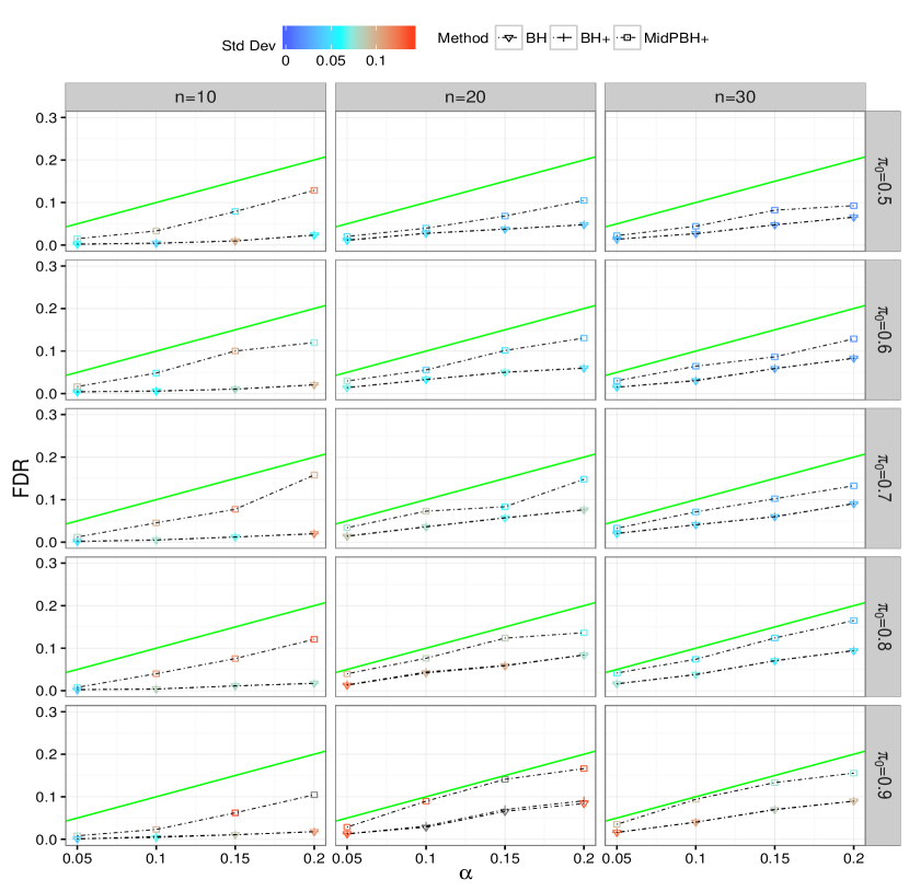
Figure 1: False discovery rate (FDR) of each procedure. The color legend “Std Dev” denotes the standard deviation of the false discovery proportion (FDP) whose expectation is FDR. The diagonal line indicates equality of the nominal FDR level $\alpha$ and the FDR of a procedure. Each procedure has been applied to two-sided p-values of Fisher’s exact tests under independence.

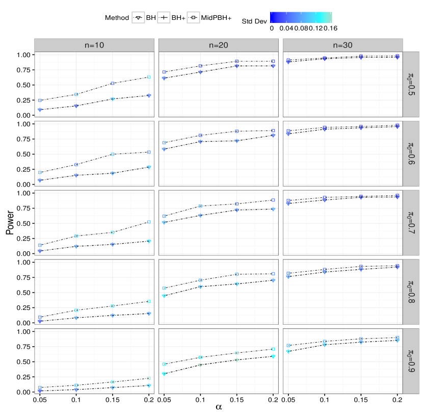
Figure 2: Power of each procedure. The color legend “Std Dev” denotes the standard deviation of the true discovery proportion (TDP) whose expectation is power. Each procedure has been applied to two-sided p-values of Fisher’s exact tests under independence.

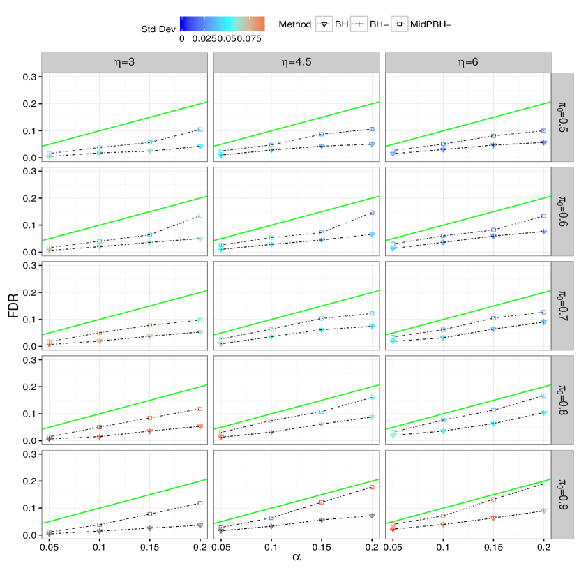
Figure 3: False discovery rate (FDR) of each procedure. The color legend “Std Dev” denotes the standard deviation of the false discovery proportion (FDP) whose expectation is FDR. The diagonal line indicates equality of the nominal FDR level $\alpha$ and the FDR of a procedure. Each procedure has been applied to two-sided p-values of Binomial tests under independence.

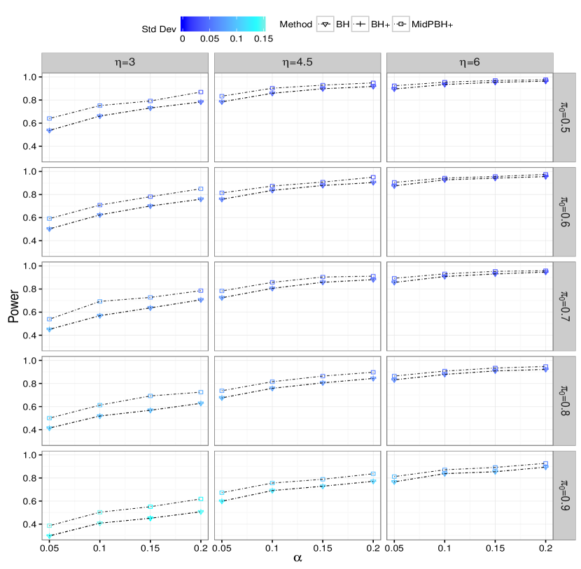
Figure 4: Power of each FDR procedure. The color legend “Std Dev” denotes the standard deviation of the true discovery proportion (TDP) whose expectation is the power. Each procedure has been applied to two-sided p-values of Binomial tests under independence.

We first summarize the results under independence. Figure 1 and Figure 3 record the FDR of each procedure. Both BH+ and MidPBH+ are conservative. Figure 2 and Figure 4 record the power of each procedure. BH+ is not less powerful than BH, and MidPBH+ is usually more powerful than BH+ and BH. The improvement in power of MidPBH+ over BH+ can be considerable for FET’s when the total number of trials for Binomial distributions is not large and for BT’s when the means of Poisson distributions are not large.

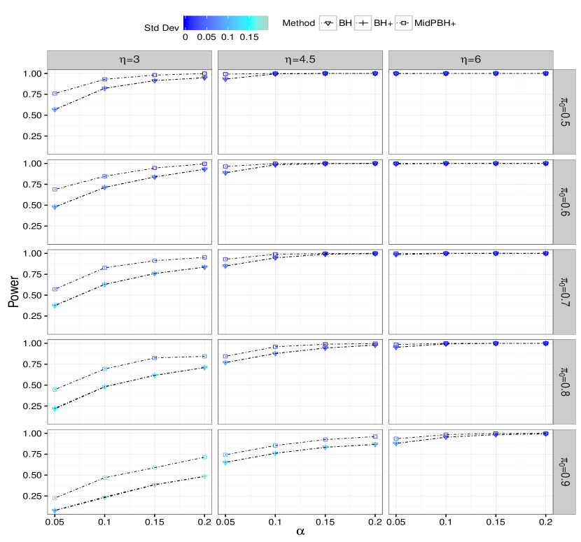
Figure 5: Power of each procedure. The color legend “Std Dev” denotes the standard deviation of the true discovery proportion (TDP) whose expectation is power. Each procedure has been applied to two-sided p-values of Binomial tests under positive dependence.

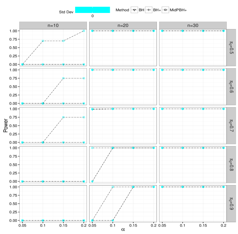
Figure 6: Power of each procedure. The color legend “Std Dev” denotes the standard deviation of the true discovery proportion (TDP) whose expectation is power. Each procedure has been applied to two-sided p-values of Fisher’s exact tests under positive dependence.

Now we summarize the results under dependence. For the simulation design stated in Section 3.2, the FDR of each procedure for each value of the triple $\left(\alpha,\pi_{0},\eta\right)$ is zero, possibly due to the positive dependence and approximately equal correlation between the generated data and moderate signal sizes under the false null hypotheses. For BT’s (see Figure 5), the powers of the procedures behave similarly to those under independence but the improvements in power of MidPBH+ over BH+ seems to be larger when Poisson random variables have smaller means. However, compared to the independence case, such improvements seem to decrease quicker as the Poisson means or the total number of trials for Binomial distributions increases. In contrast, for FET’s, the improvements in power of MidPBH+ over BH+ is either zero or enormous, likely due to the dependence among the data; see Figure 6.

4 Three applications of the BH+ procedure

We provide three applications of the BH+ procedure to multiple testing based on discrete and heterogeneous p-value distributions: one in a differential methylation study on Arabidopsis thaliana, another an HIV study, and the other a clinical safety study. BH+ applied to both conventional p-values and mid p-values, will be compared to BH applied to conventional p-values. All procedures are implemented at nominal FDR level $0.05$. The naming convention for each procedure is the same as that in Section 3.3.

4.1 Application to methylation study

The aim of the study is to identity differentially methylated cytosines between two unreplicated lines of Arabidopsis thaliana, wild-type (Col-0) and mutant defective (Met1-3). Corresponding to each cytosine, the null hypothesis is “the cytosine is not differentially methylated between the two lines”. The data set is available from Lister et al. (2008). There are $22265$ cytosines in each line, and each cytosine in each line has a discrete count that indicates its level of methylation. We choose cytosines whose total counts for both lines are greater than $10$ and whose count for each line does not exceed $25$, in order to filter out genes with unreliable low counts and to better utilize for multiple testing the jumps in the p-value distributions. This yields $2785$ cytosines, i.e., $2785$ null hypotheses to test simultaneously.

We model the counts for each cytosine in the two lines by two independent Poisson distributions, and use Binomial test to test each null hypothesis. MidPBH+ makes $531$ discoveries whereas each of BH and BH+ makes $420$, illustrating the power improvement by BH+ based on mid p-values.

4.2 Application to HIV study

The aim of the study is to identify, among $m=118$ positions, the “differentially polymorphic” positions, i.e., positions where the probability of a non-consensus amino-acid differs between two sequence sets. The two sequence sets were obtained from $n=73$ individuals infected with subtype C HIV (categorized into Group 1) and $n=73$ individuals with subtype B HIV (categorized into Group 2), respectively. The data set is available from Gilbert (2005), and how multiple testing is set up based on p-values of FET’s can also be found there. In summary, each position on the two sequence sets corresponds to a null hypothesis that “the probabilities of a non-consensus amino-acid at this position are the same between the two sequence sets”.

There are $50$ positions for which the total observed counts are identically $1$ and the corresponding two-sided p-value CDF’s are Dirac masses. To reduce the uncertainty induced by positions whose observed total counts are too low, we only analyze those whose observed total counts are at least $5$. This gives $41$ positions, i.e., $41$ null hypotheses to test. MidPBH+ makes $25$ discoveries, considerably more than $16$ made by each of BH and BH+.

4.3 Application to clinical safety study

The study aimed at differentiating adverse experiences that might have been caused by a vaccine. The study design, detailed by Mehrotra and Heyse (2004), can be summarized as follows. Participants were randomly assigned to receive the quadrivalent measles, mumps, rubella and varicella (MMRV) on day 0 (Group 1 with $148$ toddlers) or the trivalent MMR on day 0 followed by varicella on day 42 (Group 2 with $132$ toddlers). The safety profile of a vaccine is represented by reported cases for each of $40$ adverse experiences. Table 1 of Mehrotra and Heyse (2004) shows the safety profile of MMRV and that of varicella alone that were recorded for Group 1, days 0 to 42, and Group 2, days 42 to 84.

For each adverse experience, the null hypothesis is that “varicella is not associated with the adverse experience”, and FET is conducted to test if the probabilities of the adverse experience are the same between the two groups by assuming that the numbers of reported cases are realizations of two independent Binomial distributions with total numbers of trials $148$ and $132$ respectively. In this application, none of BH, BH+ and MidPBH+ claimed that varicella is not associated with any of the $40$ adverse experiences.

5 Discussion

We have proposed the BH+ procedure for FDR control for multiple testing based on p-values with càdlàg distribution functions. BH+ generalizes the BH procedure and is at least as powerful as the latter when they are applied to super-uniform p-values. Further, it is usually more powerful when applied to mid p-values than when applied to conventional p-values, and can be much so. A theoretical justification for this has been provided. Our work opens the door for multiple testing based on p-values with general distributions. Further, the BH+ procedure can be extended into weighted FDR procedures and procedures for multilayer FDR control based on p-values with càdlàg distribution functions. We leave the investigation of these to future research.

Appendices

We provide in Appendix A proofs of Theorem 1, Theorem 2 and in Appendix B simulation results under dependence.

Appendix A Proofs

A.1 Proof of Theorem 1

Let $\hat{\alpha}$ be the FDR of the BH+ procedure at nominal FDR level $\alpha\in\left(0,1\right)$. Let $b_{i,r}=\Pr\left(\left.R=r\right|p_{i}\leq\gamma_{r}\right)$ for $i\in I_{0}$ and $r\in\left\{1,...,m+1\right\}$ for which $b_{i,m+1}=0$ is set for each $i\in I_{0}$. Then the definitions of $F^{\ast}$ and $\gamma_{r}$ imply

$$\hat{\alpha}=\sum_{i\in I_{0}}\sum_{r=1}^{m}\frac{1}{r}\Pr\left(p_{i}\leq\gamma_{r}\right)b_{i,r}\leq\sum_{i\in I_{0}}\sum_{r=1}^{m}\frac{1}{r}F^{\ast}\left(\gamma_{r}\right)b_{i,r}\leq\sum_{i\in I_{0}}\sum_{r=1}^{m}\frac{\alpha}{m}b_{i,r}.$$ (6)

Let  $e_{i}\left(s,t\right)=\Pr\left(\left.R\geq s\right|p_{i}\leq t\right)$ for $i\in I_{0}$, $s\in\left\{1,...,m+1\right\}$ and $t\in\left[0,1\right]$ for which $e_{i}\left(m+1,t\right)=0$ is set for each $i\in I_{0}$ and $t\in\left[0,1\right]$. Then $b_{i,r}=e_{i}\left(r,\gamma_{r}\right)-e_{i}\left(r+1,\gamma_{r}\right)$ for each $i\in I_{0}$ and $1\leq r\leq m$. Further, the non-decreasing property of $\gamma_{r}$ in $r$ and the PRDS property of the p-values imply

$$b_{i,r}=e_{i}\left(r,\gamma_{r}\right)-e_{i}\left(r+1,\gamma_{r}\right)\leq e_{i}\left(r,\gamma_{r}\right)-e_{i}\left(r+1,\gamma_{r+1}\right).$$ (7)

So,

$$\sum_{i\in I_{0}}\sum_{r=1}^{m}\frac{\alpha}{m}b_{i,r}\leq\frac{\alpha}{m}\sum_{i\in I_{0}}\sum_{r=1}^{m}\left[e_{i}\left(r,\gamma_{r}\right)-e_{i}\left(r+1,\gamma_{r+1}\right)\right]\leq\frac{m_{0}\alpha}{m}\leq\alpha.$$ (8)

Combining (8) with (6) justifies $\hat{\alpha}\leq\alpha$.

Now we show the second claim. When $\left\{p_{i}\right\}_{i=1}^{m}$ are super-uniform, $F_{\ast}\left(t\right)\leq t$ for each $t\in\left[0,1\right]$ and $\gamma_{k}\geq\frac{\alpha k}{m}$ for each $1\leq k\leq m$. Since the BH procedure is a step-up procedure with critical values $\left\{\frac{\alpha k}{m}\right\}_{k=1}^{m}$ and rejects each $H_{i}$ if its associated p-value $p_{i}\leq\frac{\alpha R^{\prime}}{m}$ whenever

$$R^{\prime}=\max\left\{1\leq i\leq m:p_{\left(k\right)}\leq\frac{\alpha k}{m}\right\}$$

is well defined, we see that $R^{\prime}$ is upper bounded by $R$ almost surely. Namely, the set of null hypotheses rejected by the BH procedure is almost surely contained in that of the BH+ procedure. This completes the proof.

A.2 Proof of Theorem 2

Recall from Section 2.1 that $\Pr\left(P\left(X\right)\leq P\left(x\right)\right)=P\left(x\right)$ for all $x\in\mathcal{S}$ and that $\Pr\left(Q\left(X\right)\leq Q\left(x\right)\right)=P\left(x\right)$ for all $x\in\mathcal{S}$. Then, $\Pr\left(P\left(X\right)\leq t\right)\leq\Pr\left(Q\left(X\right)\leq t\right)$ for each $t\in\left[0,1\right]$. So, $F_{i}^{\mathsf{mp}}\geq F_{i}^{\mathsf{cp}}$ for each $i=1,\ldots,m$. However, $W_{\mathsf{mp}}=\max_{1\leq i\leq m}F_{i}^{\mathsf{mp}}$ and $W_{\mathsf{cp}}=\max_{1\leq i\leq m}F_{i}^{\mathsf{cp}}$. Thus, $W_{\mathsf{mp}}\geq W_{\mathsf{cp}}$. This justifies the first claim.

Let $S_{\mathsf{cp}}$ and $S_{\mathsf{mp}}$ be the support of $W_{\mathsf{cp}}$ and $W_{\mathsf{mp}}$ respectively. For each $k=1,\ldots,m$, let

$$\gamma_{k}^{\mathsf{cp}}=\max\left\{t\in S_{\mathsf{cp}}:W_{\mathsf{cp}}\left(t\right)\leq\frac{\alpha k}{m}\right\}$$

and

$$\gamma_{k}^{\mathsf{mp}}=\max\left\{t\in S_{\mathsf{mp}}:W_{\mathsf{mp}}\left(t\right)\leq\frac{\alpha k}{m}\right\}.$$

Recall $\left\{P_{\left(i\right)}\right\}_{i=1}^{m}$ as the order statistics of $\left\{P_{i}\right\}_{i=1}^{m}$ and $\left\{Q_{\left(i\right)}\right\}_{i=1}^{m}$ those of $\left\{Q_{i}\right\}_{i=1}^{m}$. Then $R_{\mathsf{cp}}=\max\left\{i:P_{\left(i\right)}\leq\gamma_{i}^{\mathsf{cp}}\right\}$ and $R_{\mathsf{mp}}=\max\left\{i:Q_{\left(i\right)}\leq\gamma_{i}^{\mathsf{mp}}\right\}$, where $R_{\mathsf{cp}}=0$ or $R_{\mathsf{mp}}=0$ is set if the set $\left\{i:P_{\left(i\right)}\leq\gamma_{i}^{\mathsf{cp}}\right\}$ or $\left\{i:Q_{\left(i\right)}\leq\gamma_{i}^{\mathsf{mp}}\right\}$ is empty, respectively.

If $R_{\mathsf{cp}}=0$, then the BH+ procedure based on $\left\{P_{i}\right\}_{i=1}^{m}$ makes no rejections, and $R_{\mathsf{mp}}\geq R_{\mathsf{cp}}$ holds automatically. It is left to consider the case where $R_{\mathsf{cp}}$ is between $1$ and $m$. Suppose (3) holds, i.e., $W_{\mathsf{mp}}\left(Q_{\left(R_{\mathsf{cp}}\right)}\right)\leq\alpha m^{-1}R_{\mathsf{cp}}$. Then $Q_{\left(R_{\mathsf{cp}}\right)}\leq\gamma_{R_{\mathsf{cp}}}^{\mathsf{mp}}$, $R_{\mathsf{mp}}$ is well defined, and $R_{\mathsf{mp}}\geq R_{\mathsf{cp}}$. On the other hand, if $R_{\mathsf{mp}}\geq R_{\mathsf{cp}}$, then $Q_{\left(R_{\mathsf{cp}}\right)}\leq\gamma_{R_{\mathsf{cp}}}^{\mathsf{mp}}$ and (3) holds. This justifies the second claim and completes the proof.

Appendix B Simulation results under positive dependence

References

- (1)
- Agresti (2002) Agresti, A. (2002). Categorical Data Analysis, 2nd edn, John Wiley & Sons, Inc., New Jersey.
- Benjamini and Hochberg (1995) Benjamini, Y. and Hochberg, Y. (1995). Controlling the false discovery rate: a practical and powerful approach to multiple testing, J. R. Statist. Soc. Ser. B 57(1): 289–300.
- Chen et al. (2018) Chen, X., Doerge, R. W. and Heyse, J. F. (2018). Multiple testing with discrete data: proportion of true null hypotheses and two adaptive FDR procedures, http://arxiv.org/abs/1410.4274; to appear in “Biometrial Journal” .
- Döhler et al. (2017) Döhler, S., Durand, G. and Roquain, E. (2017). New procedures for discrete tests with proven false discovery rate control, https://arxiv.org/abs/1706.08250v2 .
- Finner et al. (2009) Finner, H., Dickhaus, T. and Roters, M. (2009). On the false discovery rate and an asymptotically optimal rejection curve, Ann. Stat. 37(2): 596–618.
- Gilbert (2005) Gilbert, P. B. (2005). A modified false discovery rate multiple-comparisons procedure for discrete data, applied to human immunodeficiency virus genetics, J. R. Statist. Soc. Ser. C 54(1): 143–158.
- Heyse (2011) Heyse, J. F. (2011). A false discovery rate procedure for categorical data, in M. Bhattacharjee, S. K. Dhar and S. Subramanian (eds), Recent Advances in Biostatistics: False Discovery Rates, Survival Analysis, and Related Topics, chapter 3.
- Hwang and Yang (2001) Hwang, J. T. G. and Yang, M.-C. (2001). An optimality theory for mid p cvalues in contingency tables, Statistica Sinica 11(3): 807–826.
- Lancaster (1961) Lancaster, H. O. (1961). Significance tests in discrete distributions, J. Amer. Statist. Assoc. 56(294): 223–234.
- Liang (2016) Liang, K. (2016). False discovery rate estimation for large-scale homogeneous discrete p-values, Biometrics 7(2).
- Lister et al. (2008) Lister, R., O’Malley, R., Tonti-Filippini, J., Gregory, B. D., Berry, Charles C. Millar, A. H. and Ecker, J. R. (2008). Highly integrated single-base resolution maps of the epigenome in arabidopsis, Cell 133(3): 523–536.
- Mehrotra and Heyse (2004) Mehrotra, D. V. and Heyse, J. F. (2004). Use of the false discovery rate for evaluating clinical safety data, Stat. Methods Med. Res. 13(3): 227–238.
- Storey et al. (2004) Storey, J. D., Taylor, J. E. and Siegmund, D. (2004). Strong control, conservative point estimation in simultaneous conservative consistency of false discover rates: a unified approach, J. R. Statist. Soc. Ser. B 66(1): 187–205.