Parallelisation, initialisation, and boundary treatments for the diamond scheme

Abstract

We study a class of general purpose linear multisymplectic integrators for Hamiltonian wave equations based on a diamond-shaped mesh. On each diamond, the PDE is discretized by a symplectic Runge–Kutta method. The scheme advances in time by filling in each diamond locally. We demonstrate that this leads to greater efficiency and parallelization and easier treatment of boundary conditions compared to methods based on rectangular meshes. We develop a variety of initial and boundary value treatments and present numerical evidence of their performance. In all cases, the observed order of convergence is equal to or greater than the number of stages of the underlying Runge–Kutta method.

1 Introduction

The diamond scheme is a family of fully discrete numerical methods for first-order hyperbolic PDEs introduced in mclachlan2015multisymplectic . It is based on the diamond grid shown in Figure 1. The family is parameterised by its number of stages, $r$. The dependent variables are associated with each of $r$ nodes on each edge of the grid; from data on the lower two edges of a diamond, data on the top two edges can be computed locally within a single diamond. This feature is unique amongst schemes of such broad applicability and motivates its further exploration. In particular, we argued in mclachlan2015multisymplectic that the local nature of the scheme indicated that it is highly parallelizable and amenable to local boundary and initialization treatments. In this paper we present numerical evidence supporting this view.

In particular, in Section 2 we present a serial and a parallel implementation of the diamond scheme for a nonlinear wave equation. The results are exceptionally good, showing high convergence orders and almost perfect speedup with only $\gtrsim 5$ diamonds per processor. In Section 3 we develop two novel initialization methods and compare their performance to a reference method in which the diamonds are initialised with the exact solution of the differential equation. The observed orders of convergence are at least as good (and sometimes better) than those of the reference method. Dealing with this unconventional aspect of the scheme, in which initial values are not determined by the problem data, is crucial. In Section 4 we develop local boundary treatments for nonhomogeneous Dirichlet and Neumann boundary conditions. These are tested on a variety of linear and nonlinear wave equations for extremely long integration times. In all the tests in all sections, the observed order of convergence of the $r$-stage method is at least $r$, although often it exceeds this. Section 5 concludes. The method is marked by its particular theoretical advantages and by its observed performance on a range of tests.

Figure 1: Schematic of the diamond scheme for periodic boundary conditions. Information flows upwards as indicated by the solid blue arrows for a typical diamond. The solution, $\mathbf{z}$, is initialized on the solid blue zig-zag line. A step of the diamond scheme consists of two half-steps. The first half-step calculates $\mathbf{z}$ along the green dash-dot line, which by periodicity is extended to the dashed line to the right. The second half step uses the green dash-dot line to calculate the red dash-double-dotted line, which again by periodicity is extended to the left-hand dashed segment.

We describe the method as it applies to the family of Hamiltonian PDEs

$$K\mathbf{z}_{t}+L\mathbf{z}_{x}=\nabla S(\mathbf{z}),$$ (1)

where $K$ and $L$ are constant $n\times n$ real skew-symmetric matrices, $\mathbf{z}\colon\Omega\to\mathbb{R}^{n}$, $\Omega\subset\mathbb{R}^{2}$, and $S\colon\mathbb{R}^{n}\to\mathbb{R}$. Any solutions to (1) satisfy the multisymplectic conservation law

$$\omega_{t}+\kappa_{x}=0,$$ (2)

where $\omega=\frac{1}{2}(d\mathbf{z}\wedge Kd\mathbf{z})$ and $\kappa=\frac{1}{2}(d\mathbf{z}\wedge Ld\mathbf{z})$ bridges2006numerical . A numerical method that satisfies a discrete version of Eq. (2) is called a multisymplectic integrator; see bridges2006numerical ; simhamdyn for reviews of multisymplectic integration.

For ODEs, there are effective symplectic integrators—such as symplectic Runge–Kutta methods—that apply to the entire class of ODEs $Kz_{t}=\nabla S(z)$, and have excellent numerical properties, including symplecticity, arbitrary order, small error constants, unconditional stability, and linear equivariance. One generalization of these methods to the PDEs (1) is to apply high order Runge–Kutta methods in space and in time on a rectangular mesh reich . This approach inherits some of the good features listed; some of its properties, including dispersion and order behaviour, are studied in mclachlan2014on . However, the scheme does have some drawbacks. It is fully implicit, and it leads to discrete equations without a solution for periodic boundary conditions unless $r$ and $N$ (the number of cells in space) are both odd ryland ; mclachlan2014on . Solvability of the discrete equations is also affected by the boundary conditions, and no general effective treatment of boundary conditions is known for this method.

The first two issues, implicitness and boundary treatment, are related. They can be avoided for some PDEs, like the nonlinear wave equation, by applying suitably partitioned Runge–Kutta methods ryland ; mclachlan2011linear ; ryland2008multisymplecticity ; ryland2007multisymplecticity . When they apply, they lead to explicit ODEs amenable to explicit time-stepping, can have high order, and can deal with general boundary conditions. However, the partitioning means that they are not linear methods.

The diamond scheme is a different generalization of symplectic Runge–Kutta methods from ODEs to PDEs. It provides an approach that is multisymplectic, applies to all PDEs of the form (1), is linear in $z$, and is locally well-defined for any number of stages. We first give the definition of the class of diamond schemes that we will consider.

Definition 1

A diamond scheme for the PDE (1) is a quadrilateral mesh in space-time together with a mapping of each quadrilateral to a square to which a Runge–Kutta method is applied in each dimension, together with initial data specified at sufficient edge points such that the solution can be propagated forward in time by locally solving for pairs of adjacent edges.

It is convenient to first map each diamond in Figure 1 to a unit square using the linear transformation $T$ defined by (omitting unnecessary additive constants)

$$T\colon\quad\tilde{x}=\tfrac{1}{\Delta x}x+\tfrac{1}{\Delta t}t,\quad\tilde{t}=-\tfrac{1}{\Delta x}x+\tfrac{1}{\Delta t}t.$$ (3)

By the chain rule, Eq. (1) transforms to

$$\tilde{K}\tilde{\mathbf{z}}_{\tilde{t}}+\tilde{L}\tilde{\mathbf{z}}_{\tilde{x}}=\nabla S(\tilde{\mathbf{z}}),$$ (4)

where

$$\tilde{K}=\tfrac{1}{\Delta t}K-\tfrac{1}{\Delta x}L,\quad\tilde{L}=\tfrac{1}{\Delta t}K+\tfrac{1}{\Delta x}L,$$ (5)

and $\tilde{z}(\tilde{x},\tilde{t})=z(x,t)$. As the PDE (4) is still of the same class as (1), we may apply the multisymplectic Runge-Kutta collocation method given by Reich reich to Eq. (4) within a single unit square; applying $T^{-1}$ yields a method on the diamond lattice.

Let $(A,b)$ be the parameters of an $r$-stage Runge–Kutta method. In what follows, we will take the method to be the Gauss Runge–Kutta method. Figure 2 shows a diamond with $r=3$, and its transformation to the unit square. The square contains $r\times r$ internal grid points, as determined by the Runge-Kutta coefficients $c$, and internal stages $\mathbf{Z}_{i}^{j}$, which are analogous to the usual internal grid points and stages in a Runge-Kutta method. The internal stages also carry the variables $\mathbf{X}_{i}^{j}$ and $\mathbf{T}_{i}^{j}$ which approximate $z_{x}$ and $z_{t}$, respectively, at the internal stages.

The dependent variables of the method are the values of $z$ at the edge grid points.

Figure 2: The diamond transformed by a linear transformation, $T$, to the unit square. The square contains $r\times r$ ($r=3$ in this example) internal stages, $\mathbf{Z}_{i}^{j}$. The solution is known along the bottom and left hand sides. The method proceeds as two sets of $r$ Gauss Runge–Kutta $r$-stage methods: internal stage values, $\mathbf{Z}_{i}^{j},\ \mathbf{X}_{i}^{j},\ \mathbf{T}_{i}^{j}$, are calculated, then the right and top updated.

The Runge–Kutta discretization is

$$\mathbf{Z}_{i}^{j} =\tilde{\mathbf{z}}_{\ell}^{j}+\sum_{k=1}^{r}a_{ik}\mathbf{X}_{k}^{j},$$ (6)

$$\mathbf{Z}_{i}^{j} =\tilde{\mathbf{z}}^{\mathrm{b}}_{i}+\sum_{k=1}^{r}a_{jk}\mathbf{T}_{i}^{k},$$ (7)

$$\nabla S(\mathbf{Z}_{i}^{j}) =\tilde{K}\mathbf{T}_{i}^{j}+\tilde{L}\mathbf{X}_{i}^{j},$$ (8)

together with the update equations

$$\tilde{\mathbf{z}}_{\mathrm{r}}^{i} =\tilde{\mathbf{z}}_{\ell}^{i}+\sum_{k=1}^{r}b_{k}\mathbf{X}_{k}^{i},$$ (9)

$$\tilde{\mathbf{z}}^{\mathrm{t}}_{i} =\tilde{\mathbf{z}}^{\mathrm{b}}_{i}+\sum_{k=1}^{r}b_{k}\mathbf{T}_{i}^{k},$$ (10)

for $i,j=1,\dots,r$. Here $\tilde{\mathbf{z}}_{\ell}^{i}$ and $\tilde{\mathbf{z}}^{\mathrm{b}}_{i}$ are known. Eqs. (6)–(8) are first solved for the internal stage values $\mathbf{Z}_{i}^{j}$, $\mathbf{X}_{i}^{j}$, and $\mathbf{T}_{i}^{j}$, then Eqs. (9) and (10) are used to calculate $\tilde{\mathbf{z}}^{\mathrm{t}}_{i}$ and $\tilde{\mathbf{z}}_{\mathrm{r}}^{i}$. Eqs. (6)–(8) are $3r^{2}$ equations in $3r^{2}$ unknowns $\mathbf{Z}$, $\mathbf{X}$, and $\mathbf{T}$. Eqs. (6) and (7) are linear in $\mathbf{X}$ and $\mathbf{T}$. Thus in practice the method requires solving a set of $r^{2}n$ nonlinear equations for $\mathbf{Z}$ in each diamond.

The method does not use values at the corners. If necessary, solutions at the corners can be obtained using Runge–Kutta update equations along the edges, combined with averages where two edges meet.

The following basic properties of the diamond scheme are established in mclachlan2015multisymplectic . The conservation law in Theorem 2 is a discretization of the integral of $\omega_{t}+\kappa_{x}=0$ over a single diamond, transferred to the boundary of the diamond using Stokes’s theorem and discretized by Gauss quadrature.

Theorem 2

The diamond scheme satisfies the discrete symplectic conservation law

$$\frac{1}{\Delta t}\sum_{i=1}^{r}b_{i}(\omega_{i}^{\mathrm{t}}+\omega_{\mathrm{r}}^{i}-(\omega_{\ell}^{i}+\omega_{i}^{\mathrm{b}}))+\frac{1}{\Delta x}\sum_{i=1}^{r}b_{i}(\kappa_{\mathrm{r}}^{i}+\kappa_{i}^{\mathrm{b}}-(\kappa_{i}^{\mathrm{t}}+\kappa_{\ell}^{i}))=0,$$

where $\omega_{n}^{m}=\tfrac{1}{2}d\mathbf{z}_{n}^{m}\wedge Kd\mathbf{z}_{n}^{m}$, $\kappa_{n}^{m}=\tfrac{1}{2}d\mathbf{z}_{n}^{m}\wedge Ld\mathbf{z}_{n}^{m}$.

We also recall the result of mclachlan2014on that the Reich collocation scheme with the $r$-stage Gauss method, when applied on a rectangular mesh to the hyperbolic PDE (1) with initial conditions on $t=0$ and periodic boundary conditions, has global errors of order at least $r$. In some cases, order $r+1$ is observed, which is the stage order of the method. Therefore we expect convergence of order at least $r$ from the diamond scheme in cases where it is stable.

One major difference between the diamond and rectangular meshes is that the diamond mesh means that the method is effectively multi-stage. Indeed, it is the extra initial data, at different time levels, that allows the diamonds to be filled in independently. In the ODE case $L=0$, the diamond scheme yields an $r$-step integrator whose underlying 1-step method is the original Gauss method. In this paper we test the diamond scheme numerically on several different wave equations $u_{tt}-u_{xx}=f(u)$ on the domain $x\in[a,b]$, $t\in[0,T]$. The initial conditions are Cauchy (i.e., $u(x,0)$ and $u_{t}(x,0)$ are given), and various boundary conditions (periodic, Dirichlet, and Neumann) are applied at $x=a$ and $x=b$. Note that there are other methods (in particular, Lobatto IIIA–IIIB in space and an explicit symplectic splitting method in time) that perform outstandingly well on nonlinear wave equations. We adopt this equation simply as a first test: if the method fails here it is almost certainly fails overall.

The wave equation has several formulations of the form (1). Here we use the formulation with $v=u_{t}$, $w=u_{x}$, $\mathbf{z}=(u,v,w)^{T}$,

$$K=\begin{pmatrix}0&-1&0\\ 1&0&0\\ 0&0&0\end{pmatrix},\quad L=\begin{pmatrix}0&0&1\\ 0&0&0\\ -1&0&0\end{pmatrix},$$ (11)

$$\quad S(\mathbf{z})=-V(u)+\frac{1}{2}v^{2}-\frac{1}{2}w^{2},\;\mathrm{and}\;f(u)=V^{\prime}(u).$$ (12)

Then we have the following stability result.

Theorem 3

mclachlan2014on The diamond scheme with $r=1$ applied to the wave equation $u_{tt}=u_{xx}$ with periodic boundary conditions is linearly stable when $\lambda=\frac{\Delta t}{\Delta x}\leq 1$.

2 Diamond implementation

Three implementations of the diamond scheme were prepared: serial implementations in Python and C and a parallel version in C. Although the scheme is most naturally expressed using rank-3 tensors, for the implementations the tensors were flattened to matrices. Solving the nonlinear equations on each diamond requires a nonlinear solver. The Python code used the SciPy scipy routine fsolve, which is a wrapper around the minpack minpack hydrd and hybrj algorithms, which are based on the Powell hybrid method Powell01011964 . The C codes used the GNU Scientific Library gsl routines gsl_multiroot_fsolver_hybrids and gsl_multiroot_fdfsolver_gnewton which again are wrappers around the minpack hydrd and hybrj algorithms. The hydrd algorithm approximates the Jacobian, whereas hybrj requires the exact Jacobian; both versions were implemented and compared.

2.1 Convergence of the serial implementation

We first test the convergence of the serial implementation on a nonlinear wave equation. The diamond scheme with varying $r$ was used to solve the sine-Gordon equation $u_{tt}-u_{xx}=-\sin(u)$. An exact solution is the so-called breather,

$$u(x,t)=4\arctan\left(\frac{\sin\left(\frac{t}{\sqrt{2}}\right)}{\cosh\left(\frac{x}{\sqrt{2}}\right)}\right).$$ (13)

The domain is taken significantly large, $[a,b]=\left[-30,30\right]$, so the solution can be assumed to be periodic. The error is the discrete 2-norm of $u$,

$$E^{2}=\frac{b-a}{N}\sum_{i}^{N}\left(u_{i}-u(a+i\Delta x,T)\right)^{2}.$$ (14)

The number of diamonds at each time level is $N=40,80,\dots,1280$, and the integration time, $T$, is twice the largest time step. The Courant number $\frac{\Delta t}{\Delta x}=\frac{1}{2}$ is held fixed. The $2rN$ initial values of $z=(u,u_{t},u_{x})$ needed at the bottom edge of the first row of diamonds are provided by the exact solution. The results for the global error are shown in Fig. (3). It is apparent that for this problem the method converges, and the order appears to be $r$ when $r$ is odd and $r+1$ when $r$ is even.

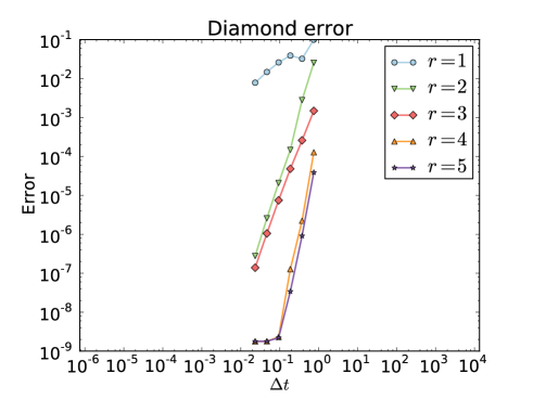
Figure 3: The error of the diamond scheme with varying $r$ applied to the multi-symplectic Hamiltonian PDE arising from the sine-Gordon equation. The true solution was the so-called breather on the domain $\left[-30,30\right]$. The Courant number is fixed at $\frac{1}{2}$ as $\Delta t$ is decreased. The order of the method appears to be $r$ when $r$ is odd and $r+1$ when $r$ is even.

2.2 Parallel implementation and speedup

In the parallel implementation of the diamond scheme, the domain is divided into strips, finite in width in the $x$ direction and potentially infinite in the $t$ direction. The width $L$ of the domain is a multiple of $\Delta x$. There are $N=\frac{L}{\Delta x}$ diamonds in each row, and $p$ processors. The $N$ diamonds are divided as equally as possible into $p$ contiguous regions. If $N$ is a multiple of $p$ then each processor will get an equal number of diamonds to work on. Otherwise $p-n$ processors get $k$ diamonds, and $n$ processors get $k+1$ diamonds, where $n=N-pk$ and $k=\lfloor\frac{N}{p}\rfloor$.

Each processor calculates the solution on its strip of diamonds. After the first half time-step (see 1) the solution at the right edge of the strip must be passed to the right-hand neighbour and received from the left. This results in $p$ transmits of vectors of length $n(r+1)$ in length. At the next half time-step the left hand edge must be passed to the left and received from the right, another $p$ transmits. If the solution is to be output each processor must send a number of values—twice the number of diamonds in its sub-domain—to one processor. This communication was achieved with an MPI gather. Since this processor has very slightly more work to perform it is desirable to ensure it is one of the $p-n$ processors that receives $k$ diamonds to work on.

To test how much the diamond scheme could benefit from running in parallel it was run on the New Zealand eScience Infrastructure’s (NeSI’s) Pan Intel Linux cluster physically located at the University of Auckland, New Zealand. At the time of use the cluster had approximately 6000 cores each running somewhere between 2GHz and 3GHz with most around 2.7GHz or 2.8GHz. Most cores had at least 10GB of RAM available, far more than we required. Due to the busyness of the cluster it was impractical to request specific CPUs for each job, thus there was a certain variability in timing tests simply because of the different speeds of the CPUs available. However the uni-processor jobs, arguably the most important while testing parallel speed-ups, did run on the most common 2.7GHz or 2.8GHz processors.

The diamond scheme was initialized with the diamond initialization method detailed in Section 3, $r$ was set to 5, the number of time steps was 1000, $\Delta t=0.05$, and the periodic sine-Gordon problem from Table 2 was used. Despite the cluster having approximately 6000 cores, by trial and error it was apparent that only about a maximum of 300 or 400 cores could be readily available on demand. So each trial consisted of nine runs with the number of cores being 1, 3, 7, 20, 56, 100, 150, 300, and 350. For each run the wall-clock time was recorded using the Unix date command, the program run, and then the wall-clock time checked again. Each trial (set of nine runs) was performed twice with a couple of days in between each trial, and the time results averaged.

According to Amdahl’s law amdahl , for a particular problem size, if $n$ is the number of cores, and $B\in[0,1]$ is the fraction of the algorithm that is strictly serial, then the theoretical time $T(n)$ for the algorithm to run on $n$ cores is

$$T(n)=T(1)\left(B+\frac{1}{n}(1-B)\right).$$

Thus the theoretical speed-up $S(n)$ is

$$S(n)=\frac{T(1)}{T(n)}=\frac{1}{B+\tfrac{1}{n}(1-B)}.$$ (15)

Letting $n\rightarrow\infty$ gives a theoretical maximum speed-up of $\tfrac{1}{B}$. By increasing $n$ until the speed-up begins to tail-off it is possible to estimate $B$. For a perfectly parallelizeable algorithm the speed-up should be equal to the number of cores used. In the first trial, shown on the left in Figure 4, $\Delta x$ was such that there were 4000 diamonds across the domain.

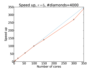
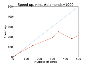
Figure 4: Speed-up of the diamond scheme versus the number of cores for the code running on the NeSI Pan cluster. Code that was perfectly parallelizeable would have the speed-up equal to the number of cores (the blue line). As the ratio of the number of cores to the amount of work (number of diamonds across the domain) increases one would expect the speed-up to deviate from the perfect blue line. On the left, with at least $4000/350>11$ diamonds per core, the speedup is very good. On the right, with as few as 2 diamonds per core, the performance deteriorates. The speed up was calculated from a single run (not an average of two runs) for the 450 and 499 number of cores runs.

As the ratio of the number of cores to the amount of work (number of diamonds across the domain) increases, one would expect the speed-up to diverge from the perfect speed-up line. This is because the overhead in communication will gradually swamp the gains in computation time. For this trial the speed-up is still very good and it is impossible to estimate $B$, the fraction of the algorithm that is strictly serial. Ideally, the number of cores would be increased until a deviation from the perfectly parallelizable line could be reliably detected, however no more cores were easily available.

So, instead of increasing the number of cores, the number of diamonds was decreased. Figure 4 (right) shows the second trial where the number of diamonds across the domain was decreased to 1000. One of the trials included two extra runs with $n=450$ and $n=499$. Because it took many days for these runs to begin executing, the second trial did not include these large runs, and no averaging could take place. This figure shows the speed-up reaching approximately 250 before beginning to tail off. So for this size of problem, from (15) this equates to $B\approx 0.4\%$, which is remarkably low. The conclusion is that the diamond scheme is exceptionally parallelizable.

3 Diamond scheme initialization

The diamond mesh creates an issue for initialization which is not present (or hardly present) for rectangular meshes. In this section we develop two initialization methods, the diamond initialization and phantom initialization methods, and compare them to a reference ‘method’ in which initial values are taken from the exact solution.

3.1 Diamond initialization method

For the nonlinear wave equations, initial conditions for $u$ and $u_{t}$ are specified at $t=0$. Differentiating with respect to $x$, we can assume that $u_{x}$, and hence all components of $z$, are known at $t=0$.

The $x$-axis cuts the first row of diamonds in half, yielding a row of triangles. In the diamond initialization method, each triangle is mapped to the unit square, then the usual set of equations (6)– (10) solved, giving values for $z$ on the top-left and top-right edges of the triangle.

The transformation, $x=\tilde{x}-\tilde{t},t=\tilde{x}\tilde{t}$, illustrated in Figure 5, takes the unit square to the triangle $(-1,0),(1,0),(0,1)$.

Figure 5: The unit square under the map $x=\tilde{x}-\tilde{t},t=\tilde{x}\tilde{t}$.

Adding a translation and scaling results in the map

$$x =\frac{\Delta x}{2}(\tilde{x}-\tilde{t})+b$$ (16)

$$t =\frac{\Delta t}{2}\tilde{x}\tilde{t}$$ (17)

which takes the unit square to the triangle $(b-\tfrac{\Delta x}{2},0),(b+\tfrac{\Delta x}{2},0),(b,\tfrac{\Delta t}{2})$. Recall that the transformed $K$ and $L$ are given by

$$\tilde{K} =g_{t}K+g_{x}L$$

$$\tilde{L} =f_{t}K+f_{x}L,$$

where $(\tilde{x},\tilde{t})=(f(x,t),g(x,t))$. This yields

$$\tilde{K} =\tfrac{2}{\Delta x\Delta t(\tilde{x}+\tilde{t})}\left(\Delta xK-\tilde{t}\Delta tL\right)$$

$$\tilde{L} =\tfrac{2}{\Delta x\Delta t(\tilde{x}+\tilde{t})}\left(\Delta xK+\tilde{x}\Delta tL\right).$$

For initializing the diamond scheme, values of $z$ are needed on the bottom zig-zag (Figure 1) spaced according to the Runge–Kutta vector $c$. Because the above map (16) and its inverse are linear on the edges, this same spacing can be used in $(\tilde{x},\tilde{t})$ space.

$r$	Order
	exact	diamond
1	1	2
2	3	3
3	3	5
4	5	5
5	5	6

Table 1: Observed order of convergence of the diamond scheme initialized with the exact solution and with the diamond scheme initialization. (Data obtained from Fig. 6.) It is apparent that for this problem the diamond initialization performs as well, or better, than the exact initialization. The order appears to be $r+1$ for most $r$ (for $r=4$ the order is $r+2$ for some reason), whereas for the exact initialization the order is $r$ ($r$ odd) and $r+1$ ($r$ even).

Figure 6 shows the error of exact and diamond initialization as $\Delta t$ is reduced while keeping the Courant number $\frac{\Delta t}{\Delta x}=\frac{1}{2}$. The integration time $T=1.5$ is twice the largest time step. It is apparent that for this problem the diamond initialization is equal, or better, than exact initialization. Table 1 shows the observed convergence order of the two initialization methods.

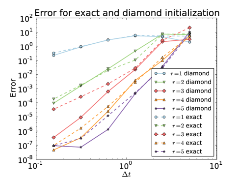
Figure 6: The error of the diamond scheme initialized using the exact and diamond methods applied to the sine-Gordon equation. The exact solution is a so-called breather on $\left[-30,30\right]$. The Courant number is fixed at $\frac{1}{2}$ as $\Delta t$ is decreased. The error is the 2-norm of the global error at the final time, Eq. 14. For this problem the diamond initialization is as accurate or better than exact initialization.

Name	Equation	Range	Solution
Esin	$u_{tt}+u_{xx}=0$	$0\leq x\leq 2\pi$	$e^{2\sin(x-t-3)}$
Sincos	$u_{tt}+u_{xx}=0$	$0\leq x\leq 2\pi$	$\sin(x)\cos(t)$
Coscos	$u_{tt}+u_{xx}=-u$	$0\leq x\leq\pi$	$\cos(2x)\cos(\sqrt{5}t)$
sine-Gordon	$u_{tt}+u_{xx}=-\sin(u)$	$-30\leq x\leq 30$	$4\arctan\left(\frac{\sin\left(\frac{t}{\sqrt{2}}\right)}{\cosh\left(\frac{x}{\sqrt{2}}\right)}\right)$

Table 2: Sample problems.

We next apply the diamond initialization method to the four different wave equations with different forcings and initial conditions given in Table 2. In each case the boundary conditions are periodic. The number of diamonds at each time level is $N=10,20,\dots,1280$, and the integration time, $T=1.5$ is twice the largest time step.

The computed global errors are shown in Figure 7. Table 3 shows the observed convergence order of the diamond scheme for these problems. It is apparent that for this problem, the order is at least $r$.

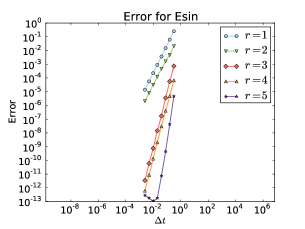
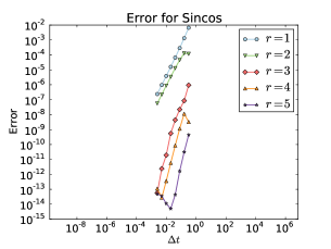
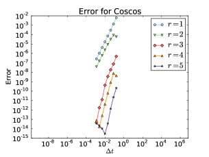
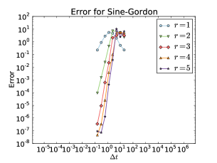
Figure 7: The error of the diamond scheme with varying number of stages $r$ applied to the Esin, Sincos, Coscos, and sine-Gordon problems (see Table 2). The Courant number is fixed at $\frac{1}{2}$ as $\Delta t$ is decreased. Table 3 summarizes the observed convergence order given by the slope of these lines.

$r$	Order
	Esin	Sincos	Coscos	sine-Gordon
1	2.0	2.1	2.1	1.8
2	1.9	1.9	1.9	4.1
3	4.0	3.4	3.3	5.6
4	3.8	3.7	3.8	5.4
5	6.2	4.8	4.6	6.8

Table 3: Observed convergence order of the problems given in Table 2 (data from Figure 7). The observed convergence order of the $r$ stage method is at least $r$.

3.2 Boundary initialization method

This method is inspired by the successful treatment of Dirichlet and Neumann boundary conditions (described in Section 4) that utilises a phantom diamond. Here a phantom diamond is constructed about the $t=0$ axis as illustrated in Figure 8.

Figure 8: An initial phantom diamond in the $r=2$ scheme. The solution, $z$, is not known on the SW or SE edges. Internally, nothing is known at the stars, and some information is known at the dashed circles. There needs to be enough known at the dashed circles to match the missing information on the SW and SE stars.

Compared to an internal diamond, the SW and SE edges are missing values of $z$; these will now become free variables, whose values will be determined by the Runge–Kutta update equations. To compensate, more information must be gathered from the initial conditions at $t=0$. Note that $r$ of the $r^{2}$ internal stages lie on $t=0$ and hence have partial data available.

By not specifying the values of $2nr$ values of $z$ on the SW and SE edges of the phantom diamond, at additional $2nr$ values must be specified at the internal stages on $t=0$. For the wave equation, $n=3$, so 6 values are required per internal stage on $t=0$ axis. The initial conditions specify $u$ and $v$ ($=u_{t}$), giving two components of $Z$ ($\approx z$) at $t=0$. The remaining required data can be obtained by differentiating the PDE. Differentiating in $x$ gives $w=u_{x}$, $v_{x}=u_{tx}$, and $w_{x}=u_{xx}$. This specifies the value of two components of $X$ ($\approx z_{x}$) at the $t=0$ internal stages. Because $u_{tx}=u_{xt}$, $w_{t}$ is also known; this specifies the value of one component of $T$ ($\approx z_{t}$). In total we now have 6 out of the 9 components of $Z$, $X$, and $T$ specified at each $t=0$ internal stage. The Runge–Kutta equations now yield a closed system that can be solved locally within each phantom diamond separately, and the update equations yield the values of $z$ on the NW and NE edges.

The boundary method does not appear to adversely affect the order of the scheme: it is at least $r$. Figure 9 shows the error for the Coscos D-N problem initialized with the usual diamond method, and the boundary method. It is apparent that the boundary initialization method does as well, or better, than the diamond initialization.

Although the boundary initialization method works well in this example, it is a little ad-hoc as it relies on being able to compute enough information from the initial conditions. This may depend on the PDE and its formulation.

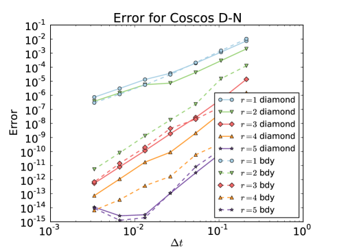
Figure 9: The error of the diamond scheme initialized with the diamond method (Section 3) and the boundary initialization method (Section 4), with varying $r$ applied to the Coscos D-N problem (see Table 4). The Courant number is fixed at $\frac{1}{2}$ as $\Delta t$ is decreased. The boundary initialization method is as good as, or better, than the diamond initialization method.

4 Dirichlet and Neumann boundary conditions

The construction of stable, high-order methods for hyperbolic initial–boundary values problems is not easy. To cite one successful approach, a significant develop effort over many years has resulted in stable finite difference methods using the summation by parts and simultaneous approximation term methods kreiss1977existence ; 2014JCoPh.268…17S ; carpenter1994time ; olsson1995summation . These finite difference operators approximate $u_{x}$ (resp. $u_{xx}$) at all points, using different finite differences near the boundary. Stability is achieved by requiring that the finite difference is skew- (resp. self-) adjoint with respect to an inner product, designed along with the method. In comparison, the compactness of the diamond scheme indicates that we might hope to construct entirely local boundary treatments, systematically for all $r$.

Figure 10: A left-hand boundary phantom diamond in the $r=2$ scheme. The solution, $z$, is known at the circles on the SE edge. For an internal diamond, $z$ would also be known at the stars on the SW edge, but not in this case. Internally, nothing is known at the stars, and some information is known at the dashed circles. There needs to be enough known at the dashed circles to match the missing information on the SW stars.

At the left and right boundaries, the geometry of the grid alters; the diamonds are cut in half to become triangles. Suppose a boundary condition specifies $k$ values of $z$. For the wave equation with Dirichlet boundary conditions, $n=3$ and $k=1$ if $u(a,t)=g(t)$ is given. Inspecting the whole diamond in Figure 10, $nr$ data values are missing on the SW edge. These need to be made up from the boundary conditions. Typically, just imposing the $k$ boundary conditions at the $r$ internal stages on $x=a$ is not sufficient to get a closed system.

We have developed and tested many approaches. A basic requirement is that the resulting method should be solvable and stable subject to a CFL condition, ideally $\Delta t/\Delta x<1$. In addition, we found that some methods that worked well on a simple test problem (e.g. the linear wave equation with homogeneous Dirichlet boundary conditions) did not work on more complicated problems. Thus, extensive testing was required. Before describing the successful method and its behaviour, we list some methods that were not robustly able to solve wave equations with a variety of boundary conditions: (i) specifying some components of $z$ at more points on the boundary than just the $r$ stages; (ii) using extra information from an adjacent interior diamond; (iii) mapping the boundary triangle to a square, as in the diamond initialisation method; and (iv) combinations of these.

The method that was ultimately successful is the following boundary scheme that we describe for Dirichlet and Neumann boundary conditions for the nonlinear wave equation. In both cases we use the phantom diamond as shown in Fig. 10, with $r$ conditions imposed at the internal stages on $x=a$, to compensate for the $r$ missing values at the SW edge. The entire set of equations (8) is then solved simultaneously, and the NE edge values filled in using the update equations (9,10). The $r$ new conditions are equations in the $3nr$ internal dependent variables $Z$ ($\approx z$), $X$ ($\approx z_{x}$), and $T$ $(\approx z_{t})$. These equations come from the boundary conditions, their derivatives with respect to $t$, and the derivatives of the PDE with respect to $x$ and $t$. However, note that we cannot use the PDE itself as it is already imposed at the internal stages.

1. For the Dirichlet boundary condition $u(a,t)=g(t)$, at the $x=a$ stages we specify the value of $u$ (1st component of $Z$); differentiate the boundary condition to get $u_{t}(a,t)=g^{\prime}(t)$, and we specify $v(a,t)=g^{\prime}(t)$ (2nd component of $Z$); differentiating again gives $u_{tt}(a,t)=g^{\prime}(t)$, which together with the PDE gives $w_{x}(a,t)=g^{\prime\prime}(t)-f^{\prime}(g(t))$ (3rd component of $X$).

2. For the Neumann boundary condition $u_{x}(a,t)=h(t)$, at the $x=a$ stages we specify $w$ (3rd component of $Z$); differentiating with respect to time gives $w_{t}=h^{\prime}(t)$ (3rd component of $T$); and by equality of mixed partial derivatives $v_{x}=w_{t}$, so we specify $v_{x}=h^{\prime}(t)$ (2nd component of $X$).

Name	Domain	Left boundary	Right boundary
Esin DD	$0.2\leq x\leq\tfrac{\pi}{3}$	Dirichlet	Dirichlet
Sincos DD	$0.2\leq x\leq\tfrac{\pi}{3}$	Dirichlet	Dirichlet
Sincos DN	$0.2\leq x\leq\tfrac{\pi}{3}$	Dirichlet	Neumann
Coscos DD	$0.2\leq x\leq\tfrac{\pi}{3}$	Dirichlet	Dirichlet
Coscos DN	$0.2\leq x\leq\tfrac{\pi}{3}$	Dirichlet	Neumann
sine-Gordon DD	$-2\leq x\leq 2$	Dirichlet	Dirichlet

Table 4: Sample non-periodic problems. See Table 2 for the exact equations and solutions. The Dirichlet boundary conditions are found using the exact solution, and the Neumann conditions by differentiating the exact solution with respect to $x$.

This boundary scheme is now applied to the four sample problems given in Table 2 with a mix of Dirichlet and Neumann boundary conditions. Table 4 summarizes the problems. In each case $10^{6}$–$10^{7}$ time steps were computed to ensure that the equations were solvable at each step and the solutions remained bounded.

Because the exact solution is known for all the sample problems it is easy to impose whatever boundary condition are desired on any spatial domain. The domains were chosen so the solutions were not periodic or symmetric in any way, because while testing other potential methods it became apparent that using ‘easy’ problems gave false confidence in the method. To ensure only one thing was tested at a time, the initialization scheme used was the diamond method. As a comparison, for one problem (Coscos DN), the boundary initialization was used. Because the domains are smaller than the periodic tests, a smaller number of diamonds was used, $N=2,4,\ldots,128$. Figure 11 shows the error for the various test problems as $\Delta t$ is decreased. From this data the observed order of convergence is summarized in Table 5.

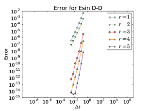
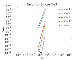
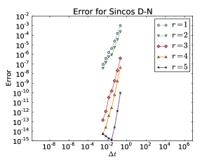
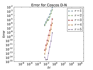
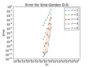
Figure 11: The error of the diamond scheme with varying $r$ applied to the Esin DD (Dirichlet/Dirichlet boundary conditions), Sincos DD, Sincos DN (Dirichlet/Neumann), Coscos DD, Coscos DN and sine-Gordon DD problems (see Table 4). The Courant number is fixed at $\frac{1}{2}$ as $\Delta t$ is decreased. Table 5 summarizes the observed convergence order given by the slope of these lines.

$r$	Order
	Esin DD	Sincos DD	Sincos DN	Coscos DD	Coscos DN	sine-Gordon DD
1	2.3	2.4	2.2	2.3	2.2	2.0
2	2.2	2.4	2.1	2.4	2.1	3.2
3	3.7	3.8	3.6	4.0	4.1	4.4
4	4.2	4.5	3.8	4.3	4.1	4.5
5	5.2	5.4	5.4	5.4	5.3	6.3

Table 5: Observed convergence orders for the initial–boundary value problems given in Table 4. To one significant figure the order appears to be $r$, although in some cases it exceeds this.

5 Conclusions

The novel diamond mesh introduced in mclachlan2015multisymplectic raised hopes that it would be suitable for parallelisation and for a wide variety of initial–boundary value problems, with local boundary closures not affecting the interior part of the scheme. We have presented numerical evidence that this is indeed possible. It still remains to prove stability and the observed orders of convergence. That this may be possible is suggested by the known results that the Reich method (for a wide class of equations of the form (1), (4)) has convergence order at least $r$, and that it also preserves discrete forms of arbitrary quadratic conservation laws, whenever the PDE has any such sun2007 .

- (1) G. M. Amdahl, Validity of the single-processor approach to achieving large scale computing capabilities, AFIPS Conference Proceedings, 30 (1967), pp. 493–485.
- (2) T. J. Bridges and S. Reich, Numerical methods for Hamiltonian PDEs, J. Phys. A, 39 (2006), pp. 5287–5320.
- (3) M. Carpenter, D. Gottlieb, and S. Abarbanel, Time-stable boundary conditions for finite-difference schemes solving hyperbolic systems: methodology and application to high-order compact schemes, Journal of Computational Physics, 111 (1994), pp. 220–236.
- (4) B. Gough and M. Galassi, GNU Scientific Library Reference Manual, Network Theory Ltd, 3 ed., 2009.
- (5) E. Jones, T. Oliphant, and P. Peterson, SciPy: Open source scientific tools for Python, 2001–. http://www.scipy.org/.
- (6) H. Kreiss and G. Scherer, On the existence of energy estimates for difference approximations for hyperbolic systems, tech. rep., Technical report, Dept. of Scientific Computing, Uppsala University, 1977.
- (7) B. Leimkuhler and S. Reich, Simulating Hamiltonian Dynamics, Cambridge Monogr. Appl. Comput. Math., Cambridge University Press, Cambridge, UK, 2004.
- (8) R. McLachlan, Y. Sun, and P. Tse, Linear stability of partitioned Runge–Kutta methods, SIAM J. Numer. Anal., 49 (2011), pp. 232–263.
- (9) R. I. McLachlan, Y. Sun, and B. Ryland, High order multisymplectic Runge–Kutta methods, SIAM J. Sci. Comput., 36 (2014), pp. A2199–A2226.
- (10) R. I. McLachlan and M. Wilkins, The multisymplectic diamond scheme, SIAM Journal on Scientific Computing, 37 (2015), pp. A369–A390.
- (11) J. J. Moré, B. S. Garbow, and K. E. Hillstrom, User Guide for MINPACK-1, ANL-80-74, Argonne National Laboratory, (1980).
- (12) P. Olsson, Summation by parts, projections, and stability. I, Mathematics of Computation, 64 (1995), pp. 1035–1065.
- (13) M. J. D. Powell, An efficient method for finding the minimum of a function of several variables without calculating derivatives, The Computer Journal, 7 (1964), pp. 155–162.
- (14) S. Reich, Multi-symplectic Runge–Kutta collocation methods for Hamiltonian wave equations, J. Comput. Phys., 157 (2000), pp. 473–499.
- (15) B. Ryland, Multisymplectic integration, PhD thesis, Massey University, New Zealand, 2007.
- (16) B. N. Ryland and R. I. McLachlan, On multisymplecticity of partitioned Runge–Kutta methods, SIAM J. Sci. Comput., 30 (2008), pp. 1318–1340.
- (17) B. N. Ryland, R. I. Mclachlan, and J. Frank, On the multisymplecticity of partitioned Runge–Kutta and splitting methods, Int. J. Comput. Math., 84 (2007), pp. 847–869.
- (18) Y. Sun, Quadratic invariants and multi-symplecticity of partitioned Runge–Kutta methods for Hamiltonian PDEs, Numerische Mathematik, 106 (2007), pp. 691–715.
- (19) M. Svärd and J. Nordström, Review of summation-by-parts schemes for initial-boundary-value problems, Journal of Computational Physics, 268 (2014), pp. 17–38.