Average Cost of QuickXsort with Pivot Sampling

Abstract

Abstract: QuickXsort is a strategy to combine Quicksort with another sorting method X, so that the result has essentially the same comparison cost as X in isolation, but sorts in place even when X requires a linear-size buffer. We solve the recurrence for QuickXsort precisely up to the linear term including the optimization to choose pivots from a sample of $k$ elements. This allows to immediately obtain overall average costs using only the average costs of sorting method X (as if run in isolation). We thereby extend and greatly simplify the analysis of QuickHeapsort and QuickMergesort with practically efficient pivot selection, and give the first tight upper bounds including the linear term for such methods.

1 Introduction

In QuickXsort [5], we use the recursive scheme of ordinary Quicksort, but instead of doing two recursive calls after partitioning, we first sort one of the segments by some other sorting method X. Only the second segment is recursively sorted by QuickXsort. The key insight is that X can use the second segment as a temporary buffer for elements. By that, QuickXsort is sorting in-place (using $O(1)$ words of extra space) even when X itself is not.

Not every method makes a suitable ‘X’; it must use the buffer in a swap-like fashion: After X has sorted its segment, the elements originally stored in our buffer must still be intact, i. e., they must still be stored in the buffer, albeit in a different order. Two possible examples that use extra space in such a way are Mergesort (see Section 6 for details) and a comparison-efficient Heapsort variant [1] with an output buffer. With QuickXsort we can make those methods sort in-place while retaining their comparison efficiency. (We lose stability, though.)

While other comparison-efficient in-place sorting methods are known (e. g. [18, 12, 9]), the ones based on QuickXsort and elementary methods X are particularly easy to implement since one can adapt existing implementations for X. In such an implementation, the tried and tested optimization to choose the pivot as the median of a small sample suggests itself to improve QuickXsort. In previous works [1, 5, 3, 6], the influence of QuickXsort on the performance of X was either studied by ad-hoc techniques that do not easily apply with general pivot sampling or it was studied for the case of very good pivots: exact medians or medians of a sample of $\sqrt{n}$ elements. Both are typically detrimental to the average performance since they add significant overhead, whereas most of the benefit of sampling is realized already for samples of very small constant sizes like $3$, $5$ or $9$. Indeed, in a very recent manuscript [6], Edelkamp and Weiß describe an optimized median-of-3 QuickMergesort implementation in C++ that outperformed the library Quicksort in std::sort.

The contribution of this paper is a general transfer theorem (Theorem 5.1) that expresses the costs of QuickXsort with median-of-$k$ sampling (for any odd constant $k$) directly in terms of the costs of X, (i. e., the costs that X needs to sort $n$ elements in isolation). We thereby obtain the first analyses of QuickMergesort and QuickHeapsort with best possible constant-coefficient bounds on the linear term under realistic sampling schemes.

Since Mergesort only needs a buffer for one of the two runs, QuickMergesort should not simply give Mergesort the smaller of the two segments to sort, but rather the largest one for which the other segments still offers sufficient buffer space. (This will be the larger segment of the two if the smaller one contains at least a third of the elements; see Section 6 for details.) Our transfer theorem covers this refined version of QuickMergesort, as well, which had not been analyzed before.

The rest of the paper is structured as follows: In Section 2, we summarize previous work on QuickXsort with a focus on contributions to its analysis. Section 3 collects mathematical facts and notations used later. In Section 4 we define QuickXsort and formulate a recurrence for its cost. Its solution is stated in Section 5. Section 6 presents the QuickMergesort as our stereotypical instantiation of QuickXsort. The proof of the transfer spreads over Sections 7 and 8. In Section 9, we apply our result to QuickHeapsort and QuickMergesort and discuss some algorithmic implications.

2 Previous Work

The idea to combine Quicksort and a secondary sorting method was suggested by Contone and Cincotti [2, 1]. They study Heapsort with an output buffer (external Heapsort), and combine it with Quicksort to QuickHeapsort. They analyze the average costs for external Heapsort in isolation and use a differencing trick for dealing with the QuickXsort recurrence; however, this technique is hard to generalize to median-of-$k$ pivots.

Diekert and Weiß [3] suggest optimizations for QuickHeapsort (some of which need extra space again), and they give better upper bounds for QuickHeapsort with random pivots and median-of-3. Their results are still not tight since they upper bound the total cost of all Heapsort calls together (using ad hoc arguments on the form of the costs for one Heapsort round), without taking the actual subproblem sizes into account that Heapsort is used on. In particular, their bound on the overall contribution of the Heapsort calls does not depend on the sampling strategy.

Edelkamp and Weiß [5] explicitly describe QuickXsort as a general design pattern and, among others, consider using Mergesort as ‘X’. They use the median of $\sqrt{n}$ elements in each round throughout to guarantee good splits with high probability. They show by induction that when X uses at most $n\lg n+cn+o(n)$ comparisons on average for some constant $c$, the number of comparisons in QuickXsort is also bounded by $n\lg n+cn+o(n)$. By combining QuickMergesort with Ford and Johnson’s MergeInsertion [8] for subproblems of logarithmic size, Edelkamp and Weiß obtained an in-place sorting method that uses on the average a close to minimal number of comparisons of $n\lg n-1.3999n+o(n)$.

In a recent follow-up manuscript [6], Edelkamp and Weiß investigated the practical performance of QuickXsort and found that a tuned median-of-3 QuickMergesort variant indeed outperformed the C++ library Quicksort. They also derive an upper bound for the average costs of their algorithm using an inductive proof; their bound is not tight.

3 Preliminaries

A comprehensive list of used notation is given in Appendix A; we mention the most important here. We use Iverson’s bracket $[\mathit{stmt}]$ to mean $1$ if $\mathit{stmt}$ is true and $0$ otherwise. $\mathbb{P}[E]$ denotes the probability of event $E$, $\mathbb{E}[X]$ the expectation of random variable $X$. We write $X\mathchoice{\mathrel{\overset{\raisebox{0.0pt}{$\scriptstyle\mathcal{D}$}}{=}}}{\mathrel{\mathchoice{\hbox{\makebox[10.55551pt][c]{\makebox[0.0pt][c]{$\displaystyle\overset{\raisebox{-4.30554pt}{$\scriptscriptstyle\mathcal{D}$}}{=}$}}}}{\hbox{\makebox[10.55551pt][c]{\makebox[0.0pt][c]{$\textstyle\overset{\raisebox{-4.30554pt}{$\scriptscriptstyle\mathcal{D}$}}{=}$}}}}{\hbox{\makebox[8.22217pt][c]{\makebox[0.0pt][c]{$\scriptstyle\overset{\raisebox{-3.01389pt}{$\scriptscriptstyle\mathcal{D}$}}{=}$}}}}{\hbox{\makebox[6.66661pt][c]{\makebox[0.0pt][c]{$\scriptscriptstyle\overset{\raisebox{-2.15277pt}{$\scriptscriptstyle\mathcal{D}$}}{=}$}}}}}}{\mathrel{\overset{\mathcal{D}}{=}}}{\mathrel{\overset{\mathcal{D}}{=}}}Y$ to denote equality in distribution.

We heavily use the beta distribution: For $\alpha,\beta\in\mathbb{R}_{>0}$, $X\mathchoice{\mathrel{\overset{\raisebox{0.0pt}{$\scriptstyle\mathcal{D}$}}{=}}}{\mathrel{\mathchoice{\hbox{\makebox[10.55551pt][c]{\makebox[0.0pt][c]{$\displaystyle\overset{\raisebox{-4.30554pt}{$\scriptscriptstyle\mathcal{D}$}}{=}$}}}}{\hbox{\makebox[10.55551pt][c]{\makebox[0.0pt][c]{$\textstyle\overset{\raisebox{-4.30554pt}{$\scriptscriptstyle\mathcal{D}$}}{=}$}}}}{\hbox{\makebox[8.22217pt][c]{\makebox[0.0pt][c]{$\scriptstyle\overset{\raisebox{-3.01389pt}{$\scriptscriptstyle\mathcal{D}$}}{=}$}}}}{\hbox{\makebox[6.66661pt][c]{\makebox[0.0pt][c]{$\scriptscriptstyle\overset{\raisebox{-2.15277pt}{$\scriptscriptstyle\mathcal{D}$}}{=}$}}}}}}{\mathrel{\overset{\mathcal{D}}{=}}}{\mathrel{\overset{\mathcal{D}}{=}}}\mathrm{Beta}(\alpha,\beta)$ if $X$ admits the density $f_{X}(z)=z^{\alpha-1}(1-z)^{\beta-1}/\mathrm{B}(\alpha,\beta)$ where $\mathrm{B}(\alpha,\beta)=\int_{0}^{1}z^{\alpha-1}(1-z)^{\beta-1}\,dz$ is the beta function. Moreover, we use the beta-binomial distribution, which is a conditional binomial distribution with the success probability being a beta-distributed random variable. If $X\mathchoice{\mathrel{\overset{\raisebox{0.0pt}{$\scriptstyle\mathcal{D}$}}{=}}}{\mathrel{\mathchoice{\hbox{\makebox[10.55551pt][c]{\makebox[0.0pt][c]{$\displaystyle\overset{\raisebox{-4.30554pt}{$\scriptscriptstyle\mathcal{D}$}}{=}$}}}}{\hbox{\makebox[10.55551pt][c]{\makebox[0.0pt][c]{$\textstyle\overset{\raisebox{-4.30554pt}{$\scriptscriptstyle\mathcal{D}$}}{=}$}}}}{\hbox{\makebox[8.22217pt][c]{\makebox[0.0pt][c]{$\scriptstyle\overset{\raisebox{-3.01389pt}{$\scriptscriptstyle\mathcal{D}$}}{=}$}}}}{\hbox{\makebox[6.66661pt][c]{\makebox[0.0pt][c]{$\scriptscriptstyle\overset{\raisebox{-2.15277pt}{$\scriptscriptstyle\mathcal{D}$}}{=}$}}}}}}{\mathrel{\overset{\mathcal{D}}{=}}}{\mathrel{\overset{\mathcal{D}}{=}}}\mathrm{BetaBin}(n,\alpha,\beta)$ then $\mathbb{P}[X=i]=\binom{n}{i}\mathrm{B}(\alpha+i,\beta+(n-i))/\mathrm{B}(\alpha,\beta)$. For a collection of its properties see [23], Section 2.4.7; one property that we use here is a local limit law showing that the normalized beta-binomial distribution converges to the beta distribution. It is reproduced as Lemma C.1 in the appendix.

For solving recurrences, we build upon Roura’s master theorems [20]. The relevant continuous master theorem is restated in the appendix (Theorem B.1).

4 QuickXsort

Let X be a sorting method that requires buffer space for storing at most $\lfloor\alpha n\rfloor$ elements (for $\alpha\in[0,1]$) to sort $n$ elements. The buffer may only be accessed by swaps so that once X has finished its work, the buffer contains the same elements as before, but in arbitrary order. Indeed, we will assume that X does not compare any buffer contents; then QuickXsort preserves randomness: if the original input is a random permutation, so will be the segments after partitioning and so will be the buffer after X has terminated.

We can then combine X with Quicksort as follows: We first randomly choose a pivot and partition the input around that pivot. This results in two contiguous segments containing the $J_{1}$ elements that are smaller than the pivot and the $J_{2}$ elements that are larger than the pivot, respectively. We exclude the space for the pivot, so $J_{1}+J_{2}=n-1$; note that since the rank of the pivot is random, so are the segment sizes $J_{1}$ and $J_{2}$. We then sort one segment by X using the other segment as a buffer, and afterwards sort the buffer segment recursively by QuickXsort.

To guarantee a sufficiently large buffer for X when it sorts $J_{r}$ ($r=1$ or $2$), we must make sure that $J_{3-r}\geq\alpha J_{r}$. In case both segments could be sorted by X, we use the larger one. The motivation behind this is that we expect an advantage from reducing the subproblem size for the recursive call as much as possible.

We consider the practically relevant version of QuickXsort, where we use as pivot the median of a sample of $k=2t+1$ elements, where $t\in\mathbb{N}_{0}$ is constant w. r. t. $n$. We think of $t$ as a design parameter of the algorithm that we have to choose. Setting $t=0$ corresponds to selecting pivots uniformly at random.

4.1 Recurrence for Expected Costs

Let $c(n)$ be the expected number of comparisons in QuickXsort on arrays of size $n$ and $x(n)$ be (an upper bound for) the expected number of comparisons in X. We will assume that $x(n)$ fulfills

$$x(n) \mathchoice{\mathrel{\;\;{=}\;\;}}{\mathrel{=}}{\mathrel{=}}{\mathrel{=}}an\lg n+bn\mathchoice{\mathbin{\;{\pm}\;}}{\mathbin{\pm}}{\mathbin{\pm}}{\mathbin{\pm}}O(n^{1-\varepsilon}),\qquad(n\to\infty),$$

for constants $a$, $b$ and $\varepsilon\in(0,1]$.

For $\alpha<1$, we obtain two cases: When the split induced by the pivot is “uneven” – namely when $\min\{J_{1},J_{2}\}<\alpha\max\{J_{1},J_{2}\}$, i. e., $\max\{J_{1},J_{2}\}>\frac{n-1}{1+\alpha}$ – the smaller segment is not large enough to be used as buffer. Then we can only assign the large segment as a buffer and run X on the smaller segment. If however the split is about “even”, i. e., both segments are $\leq\tfrac{n-1}{1+\alpha}$ we can sort the larger of the two segments by X. These cases also show up in the recurrence of costs:

$$c(n) \mathchoice{\mathrel{\;\;{=}\;\;}}{\mathrel{=}}{\mathrel{=}}{\mathrel{=}}b(n)\geq 0,\qquad(n\leq k)$$

$$c(n) \mathchoice{\mathrel{\;\;{=}\;\;}}{\mathrel{=}}{\mathrel{=}}{\mathrel{=}}\begin{aligned} (n-k)+b(k)&\mathchoice{\mathbin{\>{+}\>}}{\mathbin{+}}{\mathbin{+}}{\mathbin{+}}\mathbb{E}\left[[J_{1},J_{2}\leq\tfrac{1}{1+\alpha}(n-1)][J_{1}>J_{2}](x(J_{1})+c(J_{2}))\right]\\ &\mathchoice{\mathbin{\>{+}\>}}{\mathbin{+}}{\mathbin{+}}{\mathbin{+}}\mathbb{E}\left[[J_{1},J_{2}\leq\tfrac{1}{1+\alpha}(n-1)][J_{1}\leq J_{2}](x(J_{2})+c(J_{1}))\right]\\ &\mathchoice{\mathbin{\>{+}\>}}{\mathbin{+}}{\mathbin{+}}{\mathbin{+}}\mathbb{E}\left[[J_{2}>\tfrac{1}{1+\alpha}(n-1)](x(J_{1})+c(J_{2}))\right]\\ &\mathchoice{\mathbin{\>{+}\>}}{\mathbin{+}}{\mathbin{+}}{\mathbin{+}}\mathbb{E}\left[[J_{1}>\tfrac{1}{1+\alpha}(n-1)](x(J_{2})+c(J_{1}))\right]&\qquad(n\geq 2)\end{aligned}$$

$$\mathchoice{\mathrel{\;\;{=}\;\;}}{\mathrel{=}}{\mathrel{=}}{\mathrel{=}}\sum_{r=1}^{2}\mathbb{E}[A_{r}(J_{r})c(J_{r})]+t(n)$$ (1)

where

$$A_{1}(J) \mathchoice{\mathrel{\;\;{=}\;\;}}{\mathrel{=}}{\mathrel{=}}{\mathrel{=}}[J,J^{\prime}\leq\tfrac{1}{1+\alpha}(n-1)]\cdot[J\leq J^{\prime}]\mathchoice{\mathbin{\>{+}\>}}{\mathbin{+}}{\mathbin{+}}{\mathbin{+}}[J>\tfrac{1}{1+\alpha}(n-1)]\quad\text{with }J^{\prime}=(n-1)-J$$

$$A_{2}(J) \mathchoice{\mathrel{\;\;{=}\;\;}}{\mathrel{=}}{\mathrel{=}}{\mathrel{=}}[J,J^{\prime}\leq\tfrac{1}{1+\alpha}(n-1)]\cdot[J<J^{\prime}]\mathchoice{\mathbin{\>{+}\>}}{\mathbin{+}}{\mathbin{+}}{\mathbin{+}}[J>\tfrac{1}{1+\alpha}(n-1)]$$

$$t(n) \mathchoice{\mathrel{\;\;{=}\;\;}}{\mathrel{=}}{\mathrel{=}}{\mathrel{=}}(n-1)\mathchoice{\mathbin{\>{+}\>}}{\mathbin{+}}{\mathbin{+}}{\mathbin{+}}\mathbb{E}\left[A_{2}(J_{2})x(J_{1})\right]\mathchoice{\mathbin{\>{+}\>}}{\mathbin{+}}{\mathbin{+}}{\mathbin{+}}\mathbb{E}\left[A_{1}(J_{1})x(J_{2})\right]$$

The expectation here is taken over the choice for the random pivot, i. e., over the segment sizes $J_{1}$ resp. $J_{2}$. Note that we use both $J_{1}$ and $J_{2}$ to express the conditions in a convenient form, but actually either one is fully determined by the other via $J_{1}+J_{2}=n-1$. Note how $A_{1}$ and $A_{2}$ change roles in recursive calls and toll functions, since we always sort one segment recursively and the other segment by X.

The base cases $b(n)$ are the costs to sort inputs that are too small to sample $k$ elements. A practical choice is be to switch to Insertionsort for these, which is also used for sorting the samples. Unlike for Quicksort itself, $b(n)$ only influences the logarithmic term of costs (for constant $k$). For our asymptotic transfer theorem, we only assume $b(n)\geq 0$, the actual values are immaterial.

Distribution of Subproblem Sizes

If pivots are chosen as the median of a random sample of size $k=2t+1$, the subproblem sizes have the same distribution, $J_{1}\mathchoice{\mathrel{\overset{\raisebox{0.0pt}{$\scriptstyle\mathcal{D}$}}{=}}}{\mathrel{\mathchoice{\hbox{\makebox[10.55551pt][c]{\makebox[0.0pt][c]{$\displaystyle\overset{\raisebox{-4.30554pt}{$\scriptscriptstyle\mathcal{D}$}}{=}$}}}}{\hbox{\makebox[10.55551pt][c]{\makebox[0.0pt][c]{$\textstyle\overset{\raisebox{-4.30554pt}{$\scriptscriptstyle\mathcal{D}$}}{=}$}}}}{\hbox{\makebox[8.22217pt][c]{\makebox[0.0pt][c]{$\scriptstyle\overset{\raisebox{-3.01389pt}{$\scriptscriptstyle\mathcal{D}$}}{=}$}}}}{\hbox{\makebox[6.66661pt][c]{\makebox[0.0pt][c]{$\scriptscriptstyle\overset{\raisebox{-2.15277pt}{$\scriptscriptstyle\mathcal{D}$}}{=}$}}}}}}{\mathrel{\overset{\mathcal{D}}{=}}}{\mathrel{\overset{\mathcal{D}}{=}}}J_{2}$. Without pivot sampling, we have $J_{1}\mathchoice{\mathrel{\overset{\raisebox{0.0pt}{$\scriptstyle\mathcal{D}$}}{=}}}{\mathrel{\mathchoice{\hbox{\makebox[10.55551pt][c]{\makebox[0.0pt][c]{$\displaystyle\overset{\raisebox{-4.30554pt}{$\scriptscriptstyle\mathcal{D}$}}{=}$}}}}{\hbox{\makebox[10.55551pt][c]{\makebox[0.0pt][c]{$\textstyle\overset{\raisebox{-4.30554pt}{$\scriptscriptstyle\mathcal{D}$}}{=}$}}}}{\hbox{\makebox[8.22217pt][c]{\makebox[0.0pt][c]{$\scriptstyle\overset{\raisebox{-3.01389pt}{$\scriptscriptstyle\mathcal{D}$}}{=}$}}}}{\hbox{\makebox[6.66661pt][c]{\makebox[0.0pt][c]{$\scriptscriptstyle\overset{\raisebox{-2.15277pt}{$\scriptscriptstyle\mathcal{D}$}}{=}$}}}}}}{\mathrel{\overset{\mathcal{D}}{=}}}{\mathrel{\overset{\mathcal{D}}{=}}}\mathcal{U}[0..n-1]$, a discrete uniform distribution. If we choose pivots as medians of a sample of $k=2t+1$ elements, the value for $J_{1}$ consists of two summands: $J_{1}=t+I_{1}$. The first summand, $t$, accounts for the part of the sample that is smaller than the pivot. Those $t$ elements do not take part in the partitioning round (but they have to be included in the subproblem). $I_{1}$ is the number of elements that turned out to be smaller than the pivot during partitioning.

This latter number $I_{1}$ is random, and its distribution is $I_{1}\mathchoice{\mathrel{\overset{\raisebox{0.0pt}{$\scriptstyle\mathcal{D}$}}{=}}}{\mathrel{\mathchoice{\hbox{\makebox[10.55551pt][c]{\makebox[0.0pt][c]{$\displaystyle\overset{\raisebox{-4.30554pt}{$\scriptscriptstyle\mathcal{D}$}}{=}$}}}}{\hbox{\makebox[10.55551pt][c]{\makebox[0.0pt][c]{$\textstyle\overset{\raisebox{-4.30554pt}{$\scriptscriptstyle\mathcal{D}$}}{=}$}}}}{\hbox{\makebox[8.22217pt][c]{\makebox[0.0pt][c]{$\scriptstyle\overset{\raisebox{-3.01389pt}{$\scriptscriptstyle\mathcal{D}$}}{=}$}}}}{\hbox{\makebox[6.66661pt][c]{\makebox[0.0pt][c]{$\scriptscriptstyle\overset{\raisebox{-2.15277pt}{$\scriptscriptstyle\mathcal{D}$}}{=}$}}}}}}{\mathrel{\overset{\mathcal{D}}{=}}}{\mathrel{\overset{\mathcal{D}}{=}}}\mathrm{BetaBin}(n-k,t+1,t+1)$, a so-called beta-binomial distribution. The connection to the beta distribution is best seen by assuming $n$ independent and uniformly in $(0,1)$ distributed reals as input. They are almost surely pairwise distinct and their relative ranking is equivalent to a random permutation of $[n]$, so this assumption is w. l. o. g. for our analysis. Then, the value $P$ of the pivot in the first partitioning step has a $\mathrm{Beta}(t+1,t+1)$ distribution by definition. Conditional on that value $P=p$, $I_{1}\mathchoice{\mathrel{\overset{\raisebox{0.0pt}{$\scriptstyle\mathcal{D}$}}{=}}}{\mathrel{\mathchoice{\hbox{\makebox[10.55551pt][c]{\makebox[0.0pt][c]{$\displaystyle\overset{\raisebox{-4.30554pt}{$\scriptscriptstyle\mathcal{D}$}}{=}$}}}}{\hbox{\makebox[10.55551pt][c]{\makebox[0.0pt][c]{$\textstyle\overset{\raisebox{-4.30554pt}{$\scriptscriptstyle\mathcal{D}$}}{=}$}}}}{\hbox{\makebox[8.22217pt][c]{\makebox[0.0pt][c]{$\scriptstyle\overset{\raisebox{-3.01389pt}{$\scriptscriptstyle\mathcal{D}$}}{=}$}}}}{\hbox{\makebox[6.66661pt][c]{\makebox[0.0pt][c]{$\scriptscriptstyle\overset{\raisebox{-2.15277pt}{$\scriptscriptstyle\mathcal{D}$}}{=}$}}}}}}{\mathrel{\overset{\mathcal{D}}{=}}}{\mathrel{\overset{\mathcal{D}}{=}}}\mathrm{Bin}(n-k,p)$ has a binomial distribution; the resulting mixture is the so-called beta-binomial distribution.

For $t=0$, i. e., no sampling, we have $t+\mathrm{BetaBin}(n-k,t+1,t+1)=\mathrm{BetaBin}(n-1,1,1)$, so we recover the uniform case $\mathcal{U}[0..n-1]$.

5 The Transfer Theorem

We now state the main result of the paper: an asymptotic approximation for $c(n)$.

Theorem 5.1 (Total Cost of QuickXsort)

The expected number of comparisons needed to sort a random permutation with QuickXsort using median-of-$k$ pivots, $k=2t+1$, and a sorting method X that needs a buffer of $\lfloor\alpha n\rfloor$ elements for some constant $\alpha\in[0,1]$ to sort $n$ elements and requires on average $x(n)=an\lg n+bn\pm O(n^{1-\varepsilon})$ comparisons to do so as $n\to\infty$ for some $\varepsilon\in(0,1]$ is

$$c(n) \mathchoice{\mathrel{\;\;{=}\;\;}}{\mathrel{=}}{\mathrel{=}}{\mathrel{=}}an\lg n+\biggl{(}\frac{1}{H}-a\cdot\frac{H_{k+1}-H_{t+1}}{H\ln 2}+b\biggr{)}\cdot n\mathchoice{\mathbin{\;{\pm}\;}}{\mathbin{\pm}}{\mathbin{\pm}}{\mathbin{\pm}}O(n^{1-\varepsilon}+\log n),$$

where

$$H \mathchoice{\mathrel{\;\;{=}\;\;}}{\mathrel{=}}{\mathrel{=}}{\mathrel{=}}I_{0,\frac{\alpha}{1+\alpha}}(t+2,t+1)\mathchoice{\mathbin{\>{+}\>}}{\mathbin{+}}{\mathbin{+}}{\mathbin{+}}I_{\frac{1}{2},\frac{1}{1+\alpha}}(t+2,t+1)$$

is the expected relative subproblem size that is sorted by X. $\Box$

Here $I_{x,y}(\alpha,\beta)$ is the regularized incomplete beta function

$$I_{x,y}(\alpha,\beta) \mathchoice{\mathrel{\;\;{=}\;\;}}{\mathrel{=}}{\mathrel{=}}{\mathrel{=}}\int_{x}^{y}\frac{z^{\alpha-1}(1-z)^{\beta-1}}{\mathrm{B}(\alpha,\beta)}\,dz,\qquad(\alpha,\beta\in\mathbb{R}_{+},0\leq x\leq y\leq 1).$$

We prove Theorem 5.1 in Sections 7 and 8. To simplify the presentation, we will restrict ourselves to a stereotypical algorithm for X and its value $\alpha=\frac{1}{2}$; the given arguments, however, immediately extend to the general statement above.

6 QuickMergesort

A natural candidate for X is Mergesort: It is comparison-optimal up to the linear term (and quite close to optimal in the linear term), and needs a $\Theta(n)$-element-size buffer for practical implementations of merging.

To be usable in QuickXsort, we use a swap-based merge procedure as given in Algorithm 1.

$\proc{Merge}(A[\ell..r],m,B[b..e])$ Merges runs $A[\ell,m-1]$ and $A[m..r]$ in-place into $A[l..r]$ using scratch space $B[b..e]$ $n_{1}\leftarrow r-\ell+1$;   $n_{2}\leftarrow r-\ell+1$ Assumes $A[\ell,m-1]$ and $A[m..r]$ are sorted, $n_{1}\leq n_{2}$ and $n_{1}\leq e-b+1$. for $i=0,\ldots,n_{1}-1$ do $\proc{Swap}(A[\ell+i],B[b+i])$ end for $i_{1}\leftarrow b$;   $i_{2}\leftarrow m$; $o\leftarrow\ell$ $i_{1}<b+n_{1}$ and $i_{2}\leq r$ if $B[i_{1}]\leq A[i_{2}]$ then       $\proc{Swap}(A[o],B[i_{2}])$;   $o\leftarrow o+1$;   $i_{1}\leftarrow i_{1}+1$ else       $\proc{Swap}(A[o],A[i_{1}])$;   $o\leftarrow o+1$;   $i_{2}\leftarrow i_{2}+1$   end if while $i_{1}<b+n_{1}$ do $\proc{Swap}(A[o],B[i_{2}])$;   $o\leftarrow o+1$;   $i_{1}\leftarrow i_{1}+1$   end while

List of algorithms 1 A simple merging procedure that uses the buffer only by swaps. We move the first run $A[\ell..r]$ into the buffer $B[b..b+n_{1}-1]$ and then merge it with the second run $A[m..r]$ (still stored in the original array) into the empty slot left by the first run. By the time this first half is filled, we either have consumed enough of the second run to have space to grow the merged result, or the merging was trivial, i. e., all elements in the first run were smaller.

Note that it suffices to move the smaller of the two runs to a buffer; we use a symmetric version of Algorithm 1 when the second run is shorter. Using classical top-down or bottom-up Mergesort as described in any algorithms textbook (e. g. [22]), we thus get along with $\alpha=\frac{1}{2}$.

6.1 Average Case of Mergesort

The average number of comparisons for Mergesort has the same – optimal – leading term $n\lg n$ as in the worst and best case; and this is true for both the top-down and bottom-up variants. The coefficient of the linear term of the asymptotic expansion, though, is not a constant, but a bounded periodic function with period $\lg n$, and the functions differ for best, worst, and average case and the variants of Mergesort [21, 7, 17, 10, 11].

In this paper, we will confine ourselves to an upper bound for the average case $x(n)=an\lg n+bn\mathchoice{\mathbin{\;{\pm}\;}}{\mathbin{\pm}}{\mathbin{\pm}}{\mathbin{\pm}}O(n^{1-\varepsilon})$ with constant $b$ valid for all $n$, so we will set $b$ to the supremum of the periodic function. We leave the interesting challenge open to trace the precise behavior of the fluctuations through the recurrence, where Mergesort is used on a logarithmic number of subproblems with random sizes.

We use the following upper bounds for top-down [11] and bottom-up [17] Mergesort

$$x_{\mathrm{td}}(n) \mathchoice{\mathrel{\;\;{=}\;\;}}{\mathrel{=}}{\mathrel{=}}{\mathrel{=}}n\lg n-1.24n+2\qquad\text{and}$$ (2)

$$x_{\mathrm{bu}}(n) \mathchoice{\mathrel{\;\;{=}\;\;}}{\mathrel{=}}{\mathrel{=}}{\mathrel{=}}n\lg n-0.26n\mathchoice{\mathbin{\;{\pm}\;}}{\mathbin{\pm}}{\mathbin{\pm}}{\mathbin{\pm}}O(1).$$ (3)

7 Solving the Recurrence: Leading Term

We start with Equation (1). Since $\alpha=\frac{1}{2}$ for our Mergesort, we have $\frac{\alpha}{1+\alpha}=\frac{1}{3}$ and $\frac{1}{1+\alpha}=\frac{2}{3}$. (The following arguments are valid for general $\alpha$, including the extreme case $\alpha=1$, but in an attempt to de-clutter the presentation, we stick to $\alpha=\frac{1}{2}$ here.) We rewrite $A_{1}(J_{1})$ and $A_{2}(J_{2})$ explicitly in terms of the relative subproblem size:

$$A_{1}(J_{1}) \mathchoice{\mathrel{\;\;{=}\;\;}}{\mathrel{=}}{\mathrel{=}}{\mathrel{=}}\biggl{[}\frac{J_{1}}{n-1}\mathchoice{\mathrel{\>{\in}\>}}{\mathrel{\in}}{\mathrel{\in}}{\mathrel{\in}}\Bigl{[}\frac{1}{3},\frac{1}{2}\mathchoice{\hbox{\makebox[6.22224pt][c]{\makebox[0.0pt][c]{$\displaystyle\Bigr{]}$}}}}{\hbox{\makebox[6.22224pt][c]{\makebox[0.0pt][c]{$\textstyle\Bigr{]}$}}}}{\hbox{\makebox[6.22224pt][c]{\makebox[0.0pt][c]{$\scriptstyle\Bigr{]}$}}}}{\hbox{\makebox[6.22224pt][c]{\makebox[0.0pt][c]{$\scriptscriptstyle\Bigr{]}$}}}}\cup\Bigl{(}\frac{2}{3},1\Bigr{]}\biggr{]},$$

$$A_{2}(J_{2}) \mathchoice{\mathrel{\;\;{=}\;\;}}{\mathrel{=}}{\mathrel{=}}{\mathrel{=}}\biggl{[}\frac{J_{2}}{n-1}\mathchoice{\mathrel{\>{\in}\>}}{\mathrel{\in}}{\mathrel{\in}}{\mathrel{\in}}\Bigl{[}\frac{1}{3},\frac{1}{2}\Bigr{)}\cup\Bigl{(}\frac{2}{3},1\Bigr{]}\biggr{]}.$$

Graphically, if we view $J_{1}/(n-1)$ as a point in the unit interval, the following picture shows which subproblem is sorted recursively; (the other subproblem is sorted by Mergesort).

Obviously, we have $A_{1}+A_{2}=1$ for any choice of $J_{1}$, which corresponds to having exactly one recursive call in QuickMergesort.

7.1 The Shape Function

The expectations $\mathbb{E}[A_{r}(J_{r})c(J_{r})]$ in Equation (1) are actually finite sums over the values $0,\ldots,n-1$ that $J\colonequals J_{1}$ can attain. Recall that $J_{2}=n-1-J_{1}$ and $A_{1}(J_{1})+A_{2}(J_{2})=1$ for any value of $J$. With $J=J_{1}\mathchoice{\mathrel{\overset{\raisebox{0.0pt}{$\scriptstyle\mathcal{D}$}}{=}}}{\mathrel{\mathchoice{\hbox{\makebox[10.55551pt][c]{\makebox[0.0pt][c]{$\displaystyle\overset{\raisebox{-4.30554pt}{$\scriptscriptstyle\mathcal{D}$}}{=}$}}}}{\hbox{\makebox[10.55551pt][c]{\makebox[0.0pt][c]{$\textstyle\overset{\raisebox{-4.30554pt}{$\scriptscriptstyle\mathcal{D}$}}{=}$}}}}{\hbox{\makebox[8.22217pt][c]{\makebox[0.0pt][c]{$\scriptstyle\overset{\raisebox{-3.01389pt}{$\scriptscriptstyle\mathcal{D}$}}{=}$}}}}{\hbox{\makebox[6.66661pt][c]{\makebox[0.0pt][c]{$\scriptscriptstyle\overset{\raisebox{-2.15277pt}{$\scriptscriptstyle\mathcal{D}$}}{=}$}}}}}}{\mathrel{\overset{\mathcal{D}}{=}}}{\mathrel{\overset{\mathcal{D}}{=}}}J_{2}$, we find

$$\sum_{r=1}^{2}\mathbb{E}[A_{r}(J_{r})c(J_{r})] \mathchoice{\mathrel{\;\;{=}\;\;}}{\mathrel{=}}{\mathrel{=}}{\mathrel{=}}{}\mathchoice{\mathbin{\>{\phantom{=}}\>}}{\mathbin{\phantom{=}}}{\mathbin{\phantom{=}}}{\mathbin{\phantom{=}}}\mathbb{E}\Bigg{[}\biggl{[}\frac{J}{n-1}\mathchoice{\mathrel{\>{\in}\>}}{\mathrel{\in}}{\mathrel{\in}}{\mathrel{\in}}\Bigl{[}\frac{1}{3},\frac{1}{2}\mathchoice{\hbox{\makebox[6.22224pt][c]{\makebox[0.0pt][c]{$\displaystyle\Bigr{]}$}}}}{\hbox{\makebox[6.22224pt][c]{\makebox[0.0pt][c]{$\textstyle\Bigr{]}$}}}}{\hbox{\makebox[6.22224pt][c]{\makebox[0.0pt][c]{$\scriptstyle\Bigr{]}$}}}}{\hbox{\makebox[6.22224pt][c]{\makebox[0.0pt][c]{$\scriptscriptstyle\Bigr{]}$}}}}\cup\Bigl{(}\frac{2}{3},1\Bigr{]}\biggr{]}\cdot c(J)\Bigg{]}$$

$$\mathchoice{\mathrel{\;\;{\phantom{=}}\;\;}}{\mathrel{\phantom{=}}}{\mathrel{\phantom{=}}}{\mathrel{\phantom{=}}}{}\mathchoice{\mathbin{\>{+}\>}}{\mathbin{+}}{\mathbin{+}}{\mathbin{+}}\mathbb{E}\Bigg{[}\biggl{[}\frac{J}{n-1}\mathchoice{\mathrel{\>{\in}\>}}{\mathrel{\in}}{\mathrel{\in}}{\mathrel{\in}}\Bigl{[}\frac{1}{3},\frac{1}{2}\Bigr{)}\cup\Bigl{(}\frac{2}{3},1\Bigr{]}\biggr{]}\cdot c(J)\Bigg{]}$$

$$\mathchoice{\mathrel{\;\;{=}\;\;}}{\mathrel{=}}{\mathrel{=}}{\mathrel{=}}\sum_{j=0}^{n-1}w_{n,j}\cdot c(j),\qquad\text{where}$$

$$w_{n,j} \mathchoice{\mathrel{\;\;{=}\;\;}}{\mathrel{=}}{\mathrel{=}}{\mathrel{=}}{}\phantom{{}+{}}\mathbb{P}[J=j]\cdot\Bigl{[}\tfrac{j}{n-1}\in[\tfrac{1}{3},\tfrac{1}{2}\mathchoice{\hbox{\makebox[3.8889pt][c]{\makebox[0.0pt][c]{$\displaystyle]$}}}}{\hbox{\makebox[3.8889pt][c]{\makebox[0.0pt][c]{$\textstyle]$}}}}{\hbox{\makebox[2.72223pt][c]{\makebox[0.0pt][c]{$\scriptstyle]$}}}}{\hbox{\makebox[1.94444pt][c]{\makebox[0.0pt][c]{$\scriptscriptstyle]$}}}}\cup(\tfrac{2}{3},1]\Bigr{]}$$

$$\mathchoice{\mathrel{\;\;{\phantom{=}}\;\;}}{\mathrel{\phantom{=}}}{\mathrel{\phantom{=}}}{\mathrel{\phantom{=}}}{}+\mathbb{P}[J=j]\cdot\Bigl{[}\tfrac{j}{n-1}\in[\tfrac{1}{3},\tfrac{1}{2})\cup(\tfrac{2}{3},1]\Bigr{]}$$

$$\mathchoice{\mathrel{\;\;{=}\;\;}}{\mathrel{=}}{\mathrel{=}}{\mathrel{=}}\begin{dcases}2\cdot\mathbb{P}[J=j]&\text{if }\tfrac{j}{n-1}\in[\tfrac{1}{3},\tfrac{1}{2})\cup(\tfrac{2}{3},1]\\ 1\cdot\mathbb{P}[J=j]&\text{if }\tfrac{j}{n-1}=\tfrac{1}{2}\\ 0&\text{otherwise}\end{dcases}$$

We thus have a recurrence of the form required by the Roura’s continuous master theorem (CMT) (see Theorem B.1 in Appendix B) with the weights $w_{n,j}$ from above (Figure 1 shows an example how these weights look like).

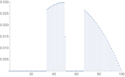
Figure 1: The weights $w_{n,j}$ for $n=101$, $t=1$; note the singular point at $j=50$.

It remains to determine $\mathbb{P}[J=j]$. Recall that we choose the pivot as the median of $k=2t+1$ elements for a fixed constant $t\in\mathbb{N}_{0}$, and the subproblem size $J$ fulfills $J=t+I$ with $I\mathchoice{\mathrel{\overset{\raisebox{0.0pt}{$\scriptstyle\mathcal{D}$}}{=}}}{\mathrel{\mathchoice{\hbox{\makebox[10.55551pt][c]{\makebox[0.0pt][c]{$\displaystyle\overset{\raisebox{-4.30554pt}{$\scriptscriptstyle\mathcal{D}$}}{=}$}}}}{\hbox{\makebox[10.55551pt][c]{\makebox[0.0pt][c]{$\textstyle\overset{\raisebox{-4.30554pt}{$\scriptscriptstyle\mathcal{D}$}}{=}$}}}}{\hbox{\makebox[8.22217pt][c]{\makebox[0.0pt][c]{$\scriptstyle\overset{\raisebox{-3.01389pt}{$\scriptscriptstyle\mathcal{D}$}}{=}$}}}}{\hbox{\makebox[6.66661pt][c]{\makebox[0.0pt][c]{$\scriptscriptstyle\overset{\raisebox{-2.15277pt}{$\scriptscriptstyle\mathcal{D}$}}{=}$}}}}}}{\mathrel{\overset{\mathcal{D}}{=}}}{\mathrel{\overset{\mathcal{D}}{=}}}\mathrm{BetaBin}(n-k,t+1,t+1)$. So we have for $i\in[0,n-1-t]$ by definition

$$\mathbb{P}[I=i] \mathchoice{\mathrel{\;\;{=}\;\;}}{\mathrel{=}}{\mathrel{=}}{\mathrel{=}}\binom{n-k}{i}\frac{\mathrm{B}\bigl{(}i+t+1,(n-k-i))+t+1\bigr{)}}{\mathrm{B}(t+1,t+1)}$$

$$\mathchoice{\mathrel{\;\;{=}\;\;}}{\mathrel{=}}{\mathrel{=}}{\mathrel{=}}\binom{n-k}{i}\frac{(t+1)^{\overline{i}}(t+1)^{\overline{n-k-i}}}{(k+1)^{\overline{n-k}}}$$

(For details, see [23, Section 2.4.7].) Now the local limit law for beta binomials (Lemma C.1 in Appendix C says that the normalized beta binomial $I/n$ converges to a beta variable “in density”, and the convergence is uniform. With the beta density $f_{P}(z)=z^{t}(1-z)^{t}/\mathrm{B}(t+1,t+1)$, we thus find by Lemma C.1 that

$$\mathbb{P}[J=j] \mathchoice{\mathrel{\;\;{=}\;\;}}{\mathrel{=}}{\mathrel{=}}{\mathrel{=}}\mathbb{P}[I=j-t]\mathchoice{\mathrel{\;\;{=}\;\;}}{\mathrel{=}}{\mathrel{=}}{\mathrel{=}}\frac{1}{n}f_{P}(j/n)\mathchoice{\mathbin{\;\;{\pm}\;\;}}{\mathbin{\pm}}{\mathbin{\pm}}{\mathbin{\pm}}O(n^{-2}),\qquad(n\to\infty).$$

The shift by the small constant $t$ from $(j-t)/n$ to $j/n$ only changes the function value by $O(n^{-1})$ since $f_{P}$ is Lipschitz continuous on $[0,1]$. (Details of that calculation are also given in [23], page 208.)

The first step towards applying the CMT is to identify a shape function $w(z)$ that approximates the relative subproblem size probabilities $w(z)\approx nw_{n,\lfloor zn\rfloor}$ for large $n$. With the above observation, a natural choice is

$$w(z) \mathchoice{\mathrel{\;\;{=}\;\;}}{\mathrel{=}}{\mathrel{=}}{\mathrel{=}}2\,\bigl{[}\tfrac{1}{3}<z<\tfrac{1}{2}\mathchoice{\mathbin{\>{\vee}\>}}{\mathbin{\vee}}{\mathbin{\vee}}{\mathbin{\vee}}z>\tfrac{2}{3}\bigr{]}\frac{z^{t}(1-z)^{t}}{\mathrm{B}(t+1,t+1)}.$$ (4)

We show in Appendix D that this is indeed a suitable shape function, i. e., it fulfills Equation (11) from the CMT.

7.2 Computing the Toll Function

The next step in applying the CMT is a leading-term approximation of the toll function. We consider a general function $x(n)=an\lg n+bn\pm O(n^{1-\varepsilon})$ where the error term holds for any constant $\varepsilon>0$ as $n\to\infty$. We start with the simple observation that

$$J\lg J \mathchoice{\mathrel{\;\;{=}\;\;}}{\mathrel{=}}{\mathrel{=}}{\mathrel{=}}J\bigl{(}\lg(\tfrac{J}{n})+\lg n\bigr{)}$$

$$\mathchoice{\mathrel{\;\;{=}\;\;}}{\mathrel{=}}{\mathrel{=}}{\mathrel{=}}n\cdot\Bigl{(}\tfrac{J}{n}\lg\tfrac{J}{n}+\tfrac{J}{n}\lg n\Bigr{)}$$

$$\mathchoice{\mathrel{\;\;{=}\;\;}}{\mathrel{=}}{\mathrel{=}}{\mathrel{=}}\tfrac{J}{n}\,n\lg n\mathchoice{\mathbin{\>{+}\>}}{\mathbin{+}}{\mathbin{+}}{\mathbin{+}}\tfrac{J}{n}\lg\bigl{(}\tfrac{J}{n}\bigr{)}\,n.$$ (5)

$$\mathchoice{\mathrel{\;\;{=}\;\;}}{\mathrel{=}}{\mathrel{=}}{\mathrel{=}}\tfrac{J}{n}\,n\lg n\mathchoice{\mathbin{\;\;{\pm}\;\;}}{\mathbin{\pm}}{\mathbin{\pm}}{\mathbin{\pm}}O(n).$$ (6)

For the leading term of $\mathbb{E}[x(J)]$, we thus only have to compute the expectation of $J/n$, which is essentially a relative subproblem size. In $t(n)$, we also have to deal with the conditionals $A_{1}(J)$ resp. $A_{2}(J)$, though. By approximating $\frac{J}{n}$ with a beta distributed variable, the conditionals translate to bounds of an integral. Details are given in Lemma E.1 (see Appendix E). This yields

$$t(n) \mathchoice{\mathrel{\;\;{=}\;\;}}{\mathrel{=}}{\mathrel{=}}{\mathrel{=}}n-1+\mathbb{E}\left[A_{2}(J_{2})x(J_{1})\right]+\mathbb{E}\left[A_{1}(J_{1})x(J_{2})\right]$$

$$\mathchoice{\mathrel{\;\;{=}\;\;}}{\mathrel{=}}{\mathrel{=}}{\mathrel{=}}a\,\mathbb{E}\left[A_{2}(J_{2})J_{1}\lg J_{1}\right]+a\,\mathbb{E}\left[A_{1}(J_{1})J_{2}\lg J_{2})\right]\mathchoice{\mathbin{\;\;{\pm}\;\;}}{\mathbin{\pm}}{\mathbin{\pm}}{\mathbin{\pm}}O(n)$$

$$\mathchoice{\mathrel{\;\;{\mathrel{\underset{\mathclap{\makebox[0.0pt][r]{\scriptsize\hyperref@@ii[lem:E-xy-Jn]{Lemma\leavevmode\nobreak\ \ref*{lem:E-xy-Jn}}}}}{=}}}\;\;}}{\mathrel{\mathrel{\underset{\mathclap{\makebox[0.0pt][r]{\scriptsize\hyperref@@ii[lem:E-xy-Jn]{Lemma\leavevmode\nobreak\ \ref*{lem:E-xy-Jn}}}}}{=}}}}{\mathrel{\mathrel{\underset{\mathclap{\makebox[0.0pt][r]{\scriptsize\hyperref@@ii[lem:E-xy-Jn]{Lemma\leavevmode\nobreak\ \ref*{lem:E-xy-Jn}}}}}{=}}}}{\mathrel{\mathrel{\underset{\mathclap{\makebox[0.0pt][r]{\scriptsize\hyperref@@ii[lem:E-xy-Jn]{Lemma\leavevmode\nobreak\ \ref*{lem:E-xy-Jn}}}}}{=}}}}2a\cdot\frac{t+1}{2t+2}\cdot\Bigl{(}I_{0,\frac{1}{3}}(t+2,t+1)+I_{\frac{1}{2},\frac{2}{3}}(t+2,t+1)\Bigr{)}\cdot n\lg n\mathchoice{\mathbin{\;\;{\pm}\;\;}}{\mathbin{\pm}}{\mathbin{\pm}}{\mathbin{\pm}}O(n)$$

$$\mathchoice{\mathrel{\;\;{=}\;\;}}{\mathrel{=}}{\mathrel{=}}{\mathrel{=}}\underbrace{a\Bigl{(}I_{0,\frac{1}{3}}(t+2,t+1)+I_{\frac{1}{2},\frac{2}{3}}(t+2,t+1)\Bigr{)}}_{\bar{a}}{}\cdot n\lg n\mathchoice{\mathbin{\;\;{\pm}\;\;}}{\mathbin{\pm}}{\mathbin{\pm}}{\mathbin{\pm}}O(n),\qquad(n\to\infty).$$ (7)

Here we use the incomplete regularized beta function

$$I_{x,y}(\alpha,\beta) \mathchoice{\mathrel{\;\;{=}\;\;}}{\mathrel{=}}{\mathrel{=}}{\mathrel{=}}\int_{x}^{y}\frac{z^{\alpha-1}(1-z)^{\beta-1}}{\mathrm{B}(\alpha,\beta)}\,dz,\qquad(\alpha,\beta\in\mathbb{R}_{+},0\leq x\leq y\leq 1)$$

for concise notation. ($I_{x,y}(\alpha,\beta)$ is the probability that a $\mathrm{Beta}(\alpha,\beta)$ distributed random variable falls into $(x,y)\subset[0,1]$, and $I_{0,x}(\alpha,\beta)$ is its cumulative distribution function.)

7.3 Which Case of the CMT?

We are now ready to apply the CMT (Theorem B.1). As shown in Section 7.2, our toll function is $\Theta(n\log n)$, so we have $\alpha=1$ and $\beta=1$. We hence compute

$$H \mathchoice{\mathrel{\;\;{=}\;\;}}{\mathrel{=}}{\mathrel{=}}{\mathrel{=}}1-\int_{0}^{1}z\,w(z)\>dz$$

$$\mathchoice{\mathrel{\;\;{=}\;\;}}{\mathrel{=}}{\mathrel{=}}{\mathrel{=}}1-\int_{0}^{1}2\,\bigl{[}\tfrac{1}{3}<z<\tfrac{1}{2}\mathchoice{\mathbin{\>{\vee}\>}}{\mathbin{\vee}}{\mathbin{\vee}}{\mathbin{\vee}}z>\tfrac{2}{3}\bigr{]}\frac{z^{t+1}(1-z)^{t}}{\mathrm{B}(t+1,t+1)}\>dz$$

$$\mathchoice{\mathrel{\;\;{=}\;\;}}{\mathrel{=}}{\mathrel{=}}{\mathrel{=}}1-2\frac{t+1}{k+1}\int_{0}^{1}\bigl{[}\tfrac{1}{3}<z<\tfrac{1}{2}\mathchoice{\mathbin{\>{\vee}\>}}{\mathbin{\vee}}{\mathbin{\vee}}{\mathbin{\vee}}z>\tfrac{2}{3}\bigr{]}\frac{z^{t+1}(1-z)^{t}}{\mathrm{B}(t+2,t+1)}\>dz$$

$$\mathchoice{\mathrel{\;\;{=}\;\;}}{\mathrel{=}}{\mathrel{=}}{\mathrel{=}}1-\Bigl{(}I_{\frac{1}{3},\frac{1}{2}}(t+2,t+1)+I_{\frac{2}{3},1}(t+2,t+1)\Bigr{)}$$

$$\mathchoice{\mathrel{\;\;{=}\;\;}}{\mathrel{=}}{\mathrel{=}}{\mathrel{=}}I_{0,\frac{1}{3}}(t+2,t+1)+I_{\frac{1}{2},\frac{2}{3}}(t+2,t+1)$$ (8)

For any sampling parameters, we have $H>0$, so the overall costs satisfy by Case 1 of Theorem B.1

$$\SwapAboveDisplaySkip c(n) \mathchoice{\mathrel{\;\;{\sim}\;\;}}{\mathrel{\sim}}{\mathrel{\sim}}{\mathrel{\sim}}\frac{t(n)}{H}\mathchoice{\mathrel{\;\;{\sim}\;\;}}{\mathrel{\sim}}{\mathrel{\sim}}{\mathrel{\sim}}\frac{\bar{a}n\lg n}{H},\qquad(n\to\infty).$$ (9)

7.4 Cancellations

Combining Equations (7) and (9), we find

$$c(n) \mathchoice{\mathrel{\;\;{\sim}\;\;}}{\mathrel{\sim}}{\mathrel{\sim}}{\mathrel{\sim}}an\lg n,\qquad(n\to\infty);$$

since $I_{0,\frac{1}{3}}+I_{\frac{1}{3},\frac{1}{2}}+I_{\frac{1}{2},\frac{2}{3}}+I_{\frac{2}{3},1}=1$. The leading term of the number of comparisons in QuickXsort is the same as in X itself, regardless of how the pivot elements are chosen! This is not as surprising as it might first seem. We are typically sorting a constant fraction of the input by X and thus only do a logarithmic number of recursive calls on a geometrically decreasing number of elements, so the linear contribution of Quicksort (partitioning and recursion cost) is dominated by even the first call of X, which has linearithmic cost. This remains true even if we allow asymmetric sampling, e. g., by choosing the pivot as the smallest (or any other order statistic) of a random sample.

Edelkamp and Weiß [5] give the above result for the case of using the median of $\sqrt{n}$ elements, where we effectively have exact medians from the perspective of analysis. In this case, the informal reasoning given above is precise, and in fact, in this case the same form of cancellations also happen for the linear term [5, Thm. 1]. (See also the “exact ranks” result in Section 9.) We will show in the following that for practical schemes of pivot sampling, i. e., with fixed sample sizes, these cancellations happen only for the leadings-term approximation. The pivot sampling scheme does affect the linear term significantly; and to measure the benefit of sampling, the analysis thus has to continue to the next term of the asymptotic expansion of $c(n)$.

Relative Subproblem Sizes

The integral $\int_{0}^{1}zw(z)\,dz$ is precisely the expected relative subproblem size for the recursive call, whereas for $t(n)$ we are interested in the subproblem that is sorted using X whose relative size is given by $\int_{0}^{1}(1-z)w(z)\,dz=1-\int_{0}^{1}zw(z)\,dz$. We can thus write $\bar{a}=aH$.

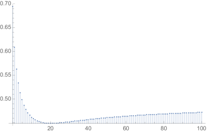
Figure 2: $\int_{0}^{1}zw(z)\,dz$, the relative recursive subproblem size, as a function of $t$.

The quantity $\int_{0}^{1}zw(z)\,dz$, the average relative size of the recursive call is of independent interest. While it is intuitively clear that for $t\to\infty$, i. e., the case of exact medians as pivots, we must have a relative subproblem size of exactly $\frac{1}{2}$, this convergence is not apparent from the behavior for finite $t$: the mass of the integral $\int_{0}^{1}zw(z)\,dz$ concentrates at $z=\frac{1}{2}$, a point of discontinuity in $w(z)$. It is also worthy of note that the expected subproblem size is initially larger than $\frac{1}{2}$ ($0.69\overline{4}$ for $t=0$), then decreases to $\approx 0.449124$ around $t=20$ and then starts to slowly increase again (see Figure 2).

8 Solving the Recurrence: The Linear Term

Since $c(n)\sim an\lg n$ for any choice of $t$, the leading term alone does not allow to make distinctions to judge the effect of sampling schemes. To compute the next term in the asymptotic expansion of $c(n)$, we consider the values $c^{\prime}(n)=c(n)-an\lg n$. $c^{\prime}(n)$ has essentially the same recursive structure as $c(n)$, only with a different toll function:

$$c^{\prime}(n) \mathchoice{\mathrel{\;\;{=}\;\;}}{\mathrel{=}}{\mathrel{=}}{\mathrel{=}}c(n)-an\lg n$$

$$\mathchoice{\mathrel{\;\;{=}\;\;}}{\mathrel{=}}{\mathrel{=}}{\mathrel{=}}\sum_{r=1}^{2}\mathbb{E}\big{[}A_{r}(J_{r})c(J_{r})\big{]}-an\lg n+t(n)$$

$$\mathchoice{\mathrel{\;\;{=}\;\;}}{\mathrel{=}}{\mathrel{=}}{\mathrel{=}}\sum_{r=1}^{2}\biggl{(}\mathbb{E}\Big{[}A_{r}(J_{r})\bigl{(}c(J_{r})-aJ_{r}\lg J_{r}\bigr{)}\Big{]}+a\,\mathbb{E}\big{[}A_{r}(J_{r})J_{r}\lg J_{r}\big{]}\biggr{)}\mathchoice{\mathbin{\>{-}\>}}{\mathbin{-}}{\mathbin{-}}{\mathbin{-}}an\lg n$$

$$\mathchoice{\mathrel{\;\;{\phantom{=}}\;\;}}{\mathrel{\phantom{=}}}{\mathrel{\phantom{=}}}{\mathrel{\phantom{=}}}\quad{}\mathchoice{\mathbin{\;{+}\;}}{\mathbin{+}}{\mathbin{+}}{\mathbin{+}}(n-1)\mathchoice{\mathbin{\>{+}\>}}{\mathbin{+}}{\mathbin{+}}{\mathbin{+}}\mathbb{E}\big{[}A_{2}(J_{2})\cdot x(J_{1})\big{]}\mathchoice{\mathbin{\>{+}\>}}{\mathbin{+}}{\mathbin{+}}{\mathbin{+}}\mathbb{E}\big{[}A_{1}(J_{1})\cdot x(J_{2})\big{]}$$

$$\mathchoice{\mathrel{\;\;{=}\;\;}}{\mathrel{=}}{\mathrel{=}}{\mathrel{=}}\sum_{r=1}^{2}\mathbb{E}\Big{[}A_{r}(J_{r})c^{\prime}(J_{r})\Big{]}+(n-1)-an\lg n$$

$$\mathchoice{\mathrel{\;\;{\phantom{=}}\;\;}}{\mathrel{\phantom{=}}}{\mathrel{\phantom{=}}}{\mathrel{\phantom{=}}}\quad{}\mathchoice{\mathbin{\>{+}\>}}{\mathbin{+}}{\mathbin{+}}{\mathbin{+}}a\,\mathbb{E}\Big{[}\bigl{(}A_{1}(J_{1})+A_{2}(J_{2})\bigr{)}J_{1}\lg J_{1}\Big{]}+b\,\mathbb{E}[A_{2}(J_{2})J_{1}]$$

$$\mathchoice{\mathrel{\;\;{\phantom{=}}\;\;}}{\mathrel{\phantom{=}}}{\mathrel{\phantom{=}}}{\mathrel{\phantom{=}}}\quad{}\mathchoice{\mathbin{\>{+}\>}}{\mathbin{+}}{\mathbin{+}}{\mathbin{+}}a\,\mathbb{E}\Big{[}\bigl{(}A_{2}(J_{2})+A_{1}(J_{1})\bigr{)}J_{2}\lg J_{2}\Big{]}+b\,\mathbb{E}[A_{1}(J_{1})J_{2}]\mathchoice{\mathbin{\;\;{\pm}\;\;}}{\mathbin{\pm}}{\mathbin{\pm}}{\mathbin{\pm}}O(n^{1-\varepsilon})$$

Since $J_{1}\mathchoice{\mathrel{\overset{\raisebox{0.0pt}{$\scriptstyle\mathcal{D}$}}{=}}}{\mathrel{\mathchoice{\hbox{\makebox[10.55551pt][c]{\makebox[0.0pt][c]{$\displaystyle\overset{\raisebox{-4.30554pt}{$\scriptscriptstyle\mathcal{D}$}}{=}$}}}}{\hbox{\makebox[10.55551pt][c]{\makebox[0.0pt][c]{$\textstyle\overset{\raisebox{-4.30554pt}{$\scriptscriptstyle\mathcal{D}$}}{=}$}}}}{\hbox{\makebox[8.22217pt][c]{\makebox[0.0pt][c]{$\scriptstyle\overset{\raisebox{-3.01389pt}{$\scriptscriptstyle\mathcal{D}$}}{=}$}}}}{\hbox{\makebox[6.66661pt][c]{\makebox[0.0pt][c]{$\scriptscriptstyle\overset{\raisebox{-2.15277pt}{$\scriptscriptstyle\mathcal{D}$}}{=}$}}}}}}{\mathrel{\overset{\mathcal{D}}{=}}}{\mathrel{\overset{\mathcal{D}}{=}}}J_{2}$ we can simplify

$$\mathchoice{\mathrel{\;\;{\phantom{=}}\;\;}}{\mathrel{\phantom{=}}}{\mathrel{\phantom{=}}}{\mathrel{\phantom{=}}}\mathbb{E}\Big{[}\bigl{(}A_{1}(J_{1})+A_{2}(J_{2})\bigr{)}J_{1}\lg J_{1}\Big{]}\mathchoice{\mathbin{\>{+}\>}}{\mathbin{+}}{\mathbin{+}}{\mathbin{+}}\mathbb{E}\Big{[}\bigl{(}A_{2}(J_{2})+A_{1}(J_{1})\bigr{)}J_{2}\lg J_{2}\Big{]}$$

$$\mathchoice{\mathrel{\;\;{=}\;\;}}{\mathrel{=}}{\mathrel{=}}{\mathrel{=}}\mathbb{E}\Big{[}\bigl{(}A_{1}(J_{1})+A_{2}(J_{2})\bigr{)}J_{1}\lg J_{1}\Big{]}\mathchoice{\mathbin{\>{+}\>}}{\mathbin{+}}{\mathbin{+}}{\mathbin{+}}\mathbb{E}\Big{[}\bigl{(}A_{2}(J_{1})+A_{1}(J_{2})\bigr{)}J_{1}\lg J_{1}\Big{]}$$

$$\mathchoice{\mathrel{\;\;{=}\;\;}}{\mathrel{=}}{\mathrel{=}}{\mathrel{=}}\mathbb{E}\Big{[}J_{1}\lg J_{1}\cdot\Bigl{(}\bigl{(}A_{1}(J_{1})+A_{1}(J_{2})\bigr{)}+\bigl{(}A_{2}(J_{1})+A_{2}(J_{2})\bigr{)}\Bigr{)}\Big{]}$$

$$\mathchoice{\mathrel{\;\;{=}\;\;}}{\mathrel{=}}{\mathrel{=}}{\mathrel{=}}2\mathbb{E}[J\lg J]$$

$$\mathchoice{\mathrel{\;\;{\mathrel{\underset{\mathclap{\makebox[0.0pt][c]{\scriptsize\eqref{eq:ex-JlnJ}}}}{=}}}\;\;}}{\mathrel{\mathrel{\underset{\mathclap{\makebox[0.0pt][c]{\scriptsize\eqref{eq:ex-JlnJ}}}}{=}}}}{\mathrel{\mathrel{\underset{\mathclap{\makebox[0.0pt][c]{\scriptsize\eqref{eq:ex-JlnJ}}}}{=}}}}{\mathrel{\mathrel{\underset{\mathclap{\makebox[0.0pt][c]{\scriptsize\eqref{eq:ex-JlnJ}}}}{=}}}}2\,\mathbb{E}[\tfrac{J}{n}]\cdot n\lg n+2\cdot\tfrac{1}{\ln 2}\mathbb{E}[\tfrac{J}{n}\ln\tfrac{J}{n}]\cdot n$$

$$\mathchoice{\mathrel{\;\;{\mathrel{\underset{\mathclap{\makebox[0.0pt][c]{\scriptsize\hyperref@@ii[lem:E-Jn-ln-Jn]{Lemma\leavevmode\nobreak\ \ref*{lem:E-Jn-ln-Jn}}}}}{=}}}\;\;}}{\mathrel{\mathrel{\underset{\mathclap{\makebox[0.0pt][c]{\scriptsize\hyperref@@ii[lem:E-Jn-ln-Jn]{Lemma\leavevmode\nobreak\ \ref*{lem:E-Jn-ln-Jn}}}}}{=}}}}{\mathrel{\mathrel{\underset{\mathclap{\makebox[0.0pt][c]{\scriptsize\hyperref@@ii[lem:E-Jn-ln-Jn]{Lemma\leavevmode\nobreak\ \ref*{lem:E-Jn-ln-Jn}}}}}{=}}}}{\mathrel{\mathrel{\underset{\mathclap{\makebox[0.0pt][c]{\scriptsize\hyperref@@ii[lem:E-Jn-ln-Jn]{Lemma\leavevmode\nobreak\ \ref*{lem:E-Jn-ln-Jn}}}}}{=}}}}n\lg n-\tfrac{1}{\ln 2}\bigl{(}H_{k+1}-H_{t+1}\bigr{)}n\mathchoice{\mathbin{\;\;{\pm}\;\;}}{\mathbin{\pm}}{\mathbin{\pm}}{\mathbin{\pm}}O(n^{1-\varepsilon}).$$

Plugging this back into our equation for $c^{\prime}(n)$, we find

$$c^{\prime}(n) \mathchoice{\mathrel{\;\;{=}\;\;}}{\mathrel{=}}{\mathrel{=}}{\mathrel{=}}\sum_{r=1}^{2}\mathbb{E}\Big{[}A_{r}(J_{r})c^{\prime}(J_{r})\Big{]}+(n-1)-an\lg n$$

$$\mathchoice{\mathrel{\;\;{\phantom{=}}\;\;}}{\mathrel{\phantom{=}}}{\mathrel{\phantom{=}}}{\mathrel{\phantom{=}}}\quad{}\mathchoice{\mathbin{\>{+}\>}}{\mathbin{+}}{\mathbin{+}}{\mathbin{+}}a\,\Bigl{(}n\lg n-\tfrac{1}{\ln 2}\bigl{(}H_{k+1}-H_{t+1}\bigr{)}n\Bigr{)}$$

$$\mathchoice{\mathrel{\;\;{\phantom{=}}\;\;}}{\mathrel{\phantom{=}}}{\mathrel{\phantom{=}}}{\mathrel{\phantom{=}}}\quad{}\mathchoice{\mathbin{\>{+}\>}}{\mathbin{+}}{\mathbin{+}}{\mathbin{+}}b\,\Bigl{(}I_{0,\frac{1}{3}}(t+2,t+1)+I_{\frac{1}{2},\frac{2}{3}}(t+2,t+1)\Bigr{)}\cdot n\mathchoice{\mathbin{\;\;{\pm}\;\;}}{\mathbin{\pm}}{\mathbin{\pm}}{\mathbin{\pm}}O(n^{1-\varepsilon})$$

$$\mathchoice{\mathrel{\;\;{=}\;\;}}{\mathrel{=}}{\mathrel{=}}{\mathrel{=}}\sum_{r=1}^{2}\mathbb{E}\Big{[}A_{r}(J_{r})c^{\prime}(J_{r})\Big{]}\mathchoice{\mathbin{\>{+}\>}}{\mathbin{+}}{\mathbin{+}}{\mathbin{+}}t^{\prime}(n)$$

where

$$t^{\prime}(n) \mathchoice{\mathrel{\;\;{=}\;\;}}{\mathrel{=}}{\mathrel{=}}{\mathrel{=}}b^{\prime}n\mathchoice{\mathbin{\;{\pm}\;}}{\mathbin{\pm}}{\mathbin{\pm}}{\mathbin{\pm}}O(n^{1-\varepsilon})$$

$$b^{\prime} \mathchoice{\mathrel{\;\;{=}\;\;}}{\mathrel{=}}{\mathrel{=}}{\mathrel{=}}1-\tfrac{a}{\ln 2}\bigl{(}H_{k+1}-H_{t+1}\bigr{)}+b\cdot H$$

Apart from the smaller toll function $t^{\prime}(n)$, this recurrence has the very same shape as the original recurrence for $c(n)$; in particular, we obtain the same shape function $w(z)$ and the same $H>0$ and obtain

$$c^{\prime}(n) \mathchoice{\mathrel{\;\;{\sim}\;\;}}{\mathrel{\sim}}{\mathrel{\sim}}{\mathrel{\sim}}\frac{t^{\prime}(n)}{H}\mathchoice{\mathrel{\;\;{\sim}\;\;}}{\mathrel{\sim}}{\mathrel{\sim}}{\mathrel{\sim}}\frac{b^{\prime}n}{H}.$$

8.1 Error Bound

Since our toll function is not given precisely, but only up to an error term $O(n^{1-\varepsilon})$ for a given fixed $\varepsilon\in(0,1]$, we also have to estimate the overall influence of this term. For that we consider the recurrence for $c(n)$ again, but replace $t(n)$ (entirely) by $C\cdot n^{1-\varepsilon}$. If $\varepsilon>0$, $\int_{0}^{1}z^{1-\varepsilon}w(z)\,dz<\int_{0}^{1}w(z)\,dz=1$, so we still find $H>0$ and apply case 1 of the CMT. The overall contribution of the error term is then $O(n^{1-\varepsilon})$. For $\varepsilon=0$, $H=0$ and case 2 applies, giving an overall error term of $O(\log n)$.

This completes the proof of Theorem 5.1.

9 Discussion

Since all our choices for X are leading-term optimal, so will QuickXsort be. We can thus fix $a=1$ in Theorem 5.1; only $b$ (and the allowable $\alpha$) still depend on X. We then basically find that going from X to QuickXsort adds a “penalty” $q$ in the linear term that depends only on the sampling size (and $\alpha$), but not on X. Table 1 shows that this penalty is $\approx n$ without sampling, but can be reduced drastically when choosing pivots from a sample of $3$ or $5$ elements. (Note that the overall costs for pivot sampling are $O(\log n)$ for constant $t$.)

	$t=0$	$t=1$	$t=2$	$t=3$	$t=10$	$t\to\infty$
$\alpha=1$	$1.1146$	$0.5070$	$0.3210$	$0.2328$	$0.07705$	$0$
$\alpha=\frac{1}{2}$	$0.9120$	$0.4050$	$0.2526$	$0.1815$	$0.05956$	$0$

Table 1: QuickXsort penalty. QuickXsort with $x(n)=n\lg n+bn$ yields $c(n)=n\lg n+(q+b)n$ where $q$, the QuickXsort penalty, is given in the table.

As we increase the sample size, we converge to the situation studied by Edelkamp and Weiß using median-of-$\sqrt{n}$, where no linear-term penalty is left [5]. Given that $q$ is less than $0.08$ already for a sample of $21$ elements, these large sample versions are mostly of theoretical interest. It is noteworthy that the improvement from no sampling to median-of-3 yields a reduction of $q$ by more than $50\%$, which is much more than its effect on Quicksort itself (where it reduces the leading term of costs by 15 % from $2n\ln n$ to $\frac{12}{7}n\ln n$).

We now apply our transfer theorem to the two most well-studied choices for X, Heapsort and Mergesort, and compare the results to analyses and measured comparison counts from previous work. The results confirm that solving the QuickXsort recurrence exactly yields much more accurate predictions for the overall number of comparisons than previous bounds that circumvented this.

9.1 QuickHeapsort

The basic external Heapsort of Cantone and Cincotti [1] always traverses one path in the heap from root to bottom and does one comparison for each edge followed, i. e., $\lfloor\lg n\rfloor$ or $\lfloor\lg n\rfloor-1$ many per deleteMax. By counting how many leaves we have on each level, Diekert and Weiß found [3, Eq. 1]

$$n\bigl{(}\lfloor\lg n\rfloor-1\bigr{)}+2\bigl{(}n-2^{\lfloor\lg n\rfloor}\bigr{)}\mathchoice{\mathbin{\>{\pm}\>}}{\mathbin{\pm}}{\mathbin{\pm}}{\mathbin{\pm}}O(\log n)\mathchoice{\mathrel{\;\;{\leq}\;\;}}{\mathrel{\leq}}{\mathrel{\leq}}{\mathrel{\leq}}n\lg n-0.913929n\mathchoice{\mathbin{\>{\pm}\>}}{\mathbin{\pm}}{\mathbin{\pm}}{\mathbin{\pm}}O(\log n)$$

comparisons for the sort-down phase. (The constant of the linear term is $1-\frac{1}{\ln 2}-\lg(2\ln 2)$, the supremum of the periodic function at the linear term). Using the classical heap construction method adds on average $1.8813726n$ comparisons [4], so here

$$x(n) \mathchoice{\mathrel{\;\;{=}\;\;}}{\mathrel{=}}{\mathrel{=}}{\mathrel{=}}n\lg n+0.967444n\mathchoice{\mathbin{\;\;{\pm}\;\;}}{\mathbin{\pm}}{\mathbin{\pm}}{\mathbin{\pm}}O(n^{\varepsilon})$$

for any $\varepsilon>0$.

Both [1] and [3] report averaged comparison counts from running time experiments. We compare them in Table 2 against the estimates from our result and previous analyses. While the approximation is not very accurate for $n=100$ (for all analyses), for larger $n$, our estimate is correct up to the first three digits, whereas previous upper bounds have almost one order of magnitude bigger errors. Note that it is expected for our bound to still be on the conservative side since we used the supremum of the periodic linear term for Heapsort.

Instance	observed	W	CC	DW
Fig. 4 [1], $n=10^{2}$, $k=1$	$806$	$+67$	$+158$	$+156$
Fig. 4 [1], $n=10^{2}$, $k=3$	$714$	$+98$	—	$+168$
Fig. 4 [1], $n=10^{5}$, $k=1$	$1\,869\,769$	$-600$	$+90\,795$	$+88\,795$
Fig. 4 [1], $n=10^{5}$, $k=3$	$1\,799\,240$	$+9\,165$	—	$+79\,324$
Fig. 4 [1], $n=10^{6}$, $k=1$	$21\,891\,874$	$+121\,748$	$+1\,035\,695$	$+1\,015\,695$
Fig. 4 [1], $n=10^{6}$, $k=3$	$21\,355\,988$	$+49\,994$	—	$+751\,581$
Tab. 2 [3], $n=10^{4}$, $k=1$	$152\,573$	$+1\,125$	$+10\,264$	$+10\,064$
Tab. 2 [3], $n=10^{4}$, $k=3$	$146\,485$	$+1\,136$	—	$+8\,152$
Tab. 2 [3], $n=10^{6}$, $k=1$	$21\,975\,912$	$+37\,710$	$+951\,657$	$+931\,657$
Tab. 2 [3], $n=10^{6}$, $k=3$	$21\,327\,478$	$+78\,504$	—	$+780\,091$

Table 2: Comparison of estimates from this paper (W), Theorem 6 of [1] (CC) and Theorem 1 of [3] (DW); shown is the difference between the estimate and the observed average.

9.2 QuickMergesort

For QuickMergesort, Edelkamp and Weiß [5, Fig. 4] report measured average comparison counts for a median-of-3 version using top-down Mergesort: the linear term is shown to be between $-0.8n$ and $-0.9n$. In a recent manuscript [6], they also analytically consider the simplified median-of-3 QuickMergesort which always sorts the smaller segment by Mergesort (i. e., $\alpha=1$). It uses $n\lg n-0.7330n+o(n)$ comparisons on average (using $b=-1.24$). They use this as a (conservative) upper bound for the original QuickMergesort.

Our transfer theorem shows that this bound is off by roughly $0.1n$: median-of-3 QuickMergesort uses at most $c(n)=n\lg n-0.8350n\pm O(\log n)$ comparisons on average. Going to median-of-5 reduces the linear term to $-0.9874n$, which is better than the worst-case for top-down Mergesort for most $n$.

Skewed Pivots for Mergesort?

For Mergesort with $\alpha=\frac{1}{2}$ the largest fraction of elements we can sort by Mergesort in one step is $\frac{2}{3}$; this suggests that using a slightly skewed pivot might be beneficial since it will increase the subproblem size for Mergesort and decrease the size for recursive calls. Indeed, Edelkamp and Weiß allude to this variation: “With about 15% the time gap, however, is not overly big, and may be bridged with additional efforts like skewed pivots and refined partitioning.” (the statement appears in the arXiv version of [5], arxiv.org/abs/1307.3033). And the above mentioned StackExchange post actually chooses pivots as the second tertile.

Our analysis above can be extended to skewed sampling schemes (omitted due to space constraints), but to illustrate this point it suffices to pay a short visit to “wishful-thinking land” and assume that we can get exact quantiles for free. We can show (e. g., with Roura’s discrete master theorem [20]) that if we always pick the exact $\rho$-quantile of the input, for $\rho\in(0,1)$, the overall costs are

$$c_{\rho}(n)\mathchoice{\mathrel{\;\;{=}\;\;}}{\mathrel{=}}{\mathrel{=}}{\mathrel{=}}\begin{dcases*}n\lg n+\biggl{(}\frac{1+h(\rho)}{1-\rho}+b\biggr{)}n\mathchoice{\mathbin{\;{\pm}\;}}{\mathbin{\pm}}{\mathbin{\pm}}{\mathbin{\pm}}O(n^{1-\varepsilon})&if $\rho\in(\frac{1}{3},\frac{1}{2})\cup(\frac{2}{3},1)$\\ n\lg n+\biggl{(}\frac{1+h(\rho)}{\rho}+b\biggr{)}n\mathchoice{\mathbin{\;{\pm}\;}}{\mathbin{\pm}}{\mathbin{\pm}}{\mathbin{\pm}}O(n^{1-\varepsilon})&otherwise\end{dcases*}$$

for $h(x)=x\lg x+(1-x)\lg(1-x)$. The coefficient of the linear term has a strict minimum at $\rho=\frac{1}{2}$: Even for $\alpha=\frac{1}{2}$, the best choice is to use the median of a sample. (The result is the same for fixed-size samples.) For QuickMergesort, skewed pivots turn out to be a pessimization, despite the fact that we sort a larger part by Mergesort. A possible explanation is that skewed pivots significantly decrease the amount of information we obtain from the comparisons during partitioning, but do not make partitioning any cheaper.

9.3 Future Work

More promising than skewed pivot sampling is the use of several pivots. The resulting MultiwayQuickXsort would be able to sort all but one segment using X and recurse on only one subproblem. Here, determining the expected subproblem sizes becomes a challenge, in particular for $\alpha<1$; we leave this for future work.

We also confined ourselves to the expected number of comparisons here, but more details about the distribution of costs are possible to obtain. The variance follows a similar recurrence as the one studied in this paper and a distributional recurrence for the costs can be given. The discontinuities in the subproblem sizes add a new facet to these analyses.

Finally, it is a typical phenomenon that constant-factor optimal sorting methods exhibit periodic linear terms. QuickXsort inherits these fluctuations but smooths them through the random subproblem sizes. Explicitly accounting for these effects is another interesting challenge for future work.

Appendix A Notation

A.1 Generic Mathematics

• natural numbers $\mathbb{N}=\{1,2,3,\ldots\}$, $\mathbb{N}_{0}=\mathbb{N}\cup\{0\}$, integers $\mathbb{Z}=\{\ldots,-2,-1,0,1,2,\ldots\}$, real numbers $\mathbb{R}$.

• restricted sets $X_{\mathrm{pred}}=\{x\in X:x\text{ fulfills }\mathrm{pred}\}$.

• repeating decimal; $0.\overline{3}=0.333\ldots=\frac{1}{3}$;
  numerals under the line form the repeated part of the decimal number.

• natural and binary logarithm; $\ln(n)=\log_{e}(n)$, $\lg(n)=\log_{2}(n)$.

• to emphasize that $X$ is a random variable it is Capitalized.

• real intervals, the end points with round parentheses are excluded, those with square brackets are included.

• integer intervals, $[m..n]=\{m,m+1,\ldots,n\}$; $[n]=[1..n]$.

• Iverson bracket, $[\text{stmt}]=1$ if stmt is true, $[\text{stmt}]=0$ otherwise.

• $n$th harmonic number; $H_{n}=\sum_{i=1}^{n}1/i$.

• $x$ with absolute error $|y|$; formally the interval $x\pm y=[x-|y|,x+|y|]$; as with $O$-terms, we use one-way equalities $z=x\pm y$ instead of $z\in x\pm y$.

• the beta function, $\mathrm{B}(\alpha,\beta)=\int_{0}^{1}z^{\alpha-1}(1-z)^{\beta-1}\,dz$

• the regularized incomplete beta function; $I_{x,y}(\alpha,\beta)=\int_{x}^{y}\frac{z^{\alpha-1}(1-z)^{\beta-1}}{\mathrm{B}(\alpha,\beta)}\,dz$ for $\alpha,\beta\in\mathbb{R}_{+}$, $0\leq x\leq y\leq 1$.

• factorial powers; “$a$ to the $b$ falling resp. rising.”

A.2 Stochastics-related Notation

• probability of an event $E$ resp. probability for random variable $X$ to attain value $x$.

• expected value of $X$; we write $\mathbb{E}[X\nonscript\>|\nonscript\>\mathopen{}Y]$ for the conditional expectation of $X$ given $Y$, and $\mathbb{E}_{#1}[f(X)]$ to emphasize that expectation is taken w. r. t. random variable $X$.

• equality in distribution; $X$ and $Y$ have the same distribution.

• uniformly in $(a,b)\subset\mathbb{R}$ distributed random variable.

• Beta distributed random variable with shape parameters $\alpha\in\mathbb{R}_{>0}$ and $\beta\in\mathbb{R}_{>0}$.

• binomial distributed random variable with $n\in\mathbb{N}_{0}$ trials and success probability $p\in[0,1]$.
  

• beta-binomial distributed random variable; $n\in\mathbb{N}_{0}$, $\alpha,\beta\in\mathbb{R}_{>0}$;

A.3 Notation for the Algorithm

• length of the input array, i. e., the input size.

• sample size $k\in\mathbb{N}_{\geq 1}$, odd; $k=2t+1$, $t\in\mathbb{N}_{0}$.

• Average costs of X, $x(n)=an\lg n+bn\pm O(n^{1-\varepsilon})$.

• toll function $t(n)=\bar{a}n\lg n+\bar{b}n\pm O(n^{1-\varepsilon})$

• (random) subproblem sizes; $J_{1}+J_{2}=n-1$; $J_{1}=t+I_{1}$;

• (random) segment sizes in partitioning; $I_{1}\mathchoice{\mathrel{\overset{\raisebox{0.0pt}{$\scriptstyle\mathcal{D}$}}{=}}}{\mathrel{\mathchoice{\hbox{\makebox[9.50002pt][c]{\makebox[0.0pt][c]{$\displaystyle\overset{\raisebox{-3.87498pt}{$\scriptscriptstyle\mathcal{D}$}}{=}$}}}}{\hbox{\makebox[9.50002pt][c]{\makebox[0.0pt][c]{$\textstyle\overset{\raisebox{-3.87498pt}{$\scriptscriptstyle\mathcal{D}$}}{=}$}}}}{\hbox{\makebox[7.40001pt][c]{\makebox[0.0pt][c]{$\scriptstyle\overset{\raisebox{-2.7125pt}{$\scriptscriptstyle\mathcal{D}$}}{=}$}}}}{\hbox{\makebox[6.0pt][c]{\makebox[0.0pt][c]{$\scriptscriptstyle\overset{\raisebox{-1.93748pt}{$\scriptscriptstyle\mathcal{D}$}}{=}$}}}}}}{\mathrel{\overset{\mathcal{D}}{=}}}{\mathrel{\overset{\mathcal{D}}{=}}}\mathrm{BetaBin}(n-k,t+1,t+1)$; $I_{2}=n-k-I_{1}$; $J_{1}=t+I_{1}$

Appendix B The Continuous Master Theorem

We restate Roura’s CMT here for convenience.

Theorem B.1 (Roura’s Continuous Master Theorem (CMT))

Let $F_{n}$ be recursively defined by

$$F_{n}\mathchoice{\mathrel{\;\;{=}\;\;}}{\mathrel{=}}{\mathrel{=}}{\mathrel{=}}\begin{dcases*}b_{n}\>,&for $0\leq n<N$;\\ \vphantom{\bigg{|}}t_{n}\mathchoice{\mathbin{\>{+}\>}}{\mathbin{+}}{\mathbin{+}}{\mathbin{+}}\smash{\sum_{j=0}^{n-1}w_{n,j}\,F_{j}},&for $n\geq N$\,,\end{dcases*}$$ (10)

where $t_{n}$, the toll function, satisfies $t_{n}\sim Kn^{\alpha}\log^{\beta}(n)$ as $n\to\infty$ for constants $K\neq 0$, $\alpha\geq 0$ and $\beta>-1$. Assume there exists a function $w:[0,1]\to\mathbb{R}_{\geq 0}$, the shape function, with $\int_{0}^{1}w(z)dz\geq 1$ and

$$\sum_{j=0}^{n-1}\,\biggl{|}w_{n,j}\mathchoice{\mathbin{\>{-}\>}}{\mathbin{-}}{\mathbin{-}}{\mathbin{-}}\!\int_{j/n}^{(j+1)/n}\mkern-15.0muw(z)\>dz\biggr{|}\mathchoice{\mathrel{\;\;{=}\;\;}}{\mathrel{=}}{\mathrel{=}}{\mathrel{=}}O(n^{-d}),\qquad(n\to\infty),$$ (11)

for a constant $d>0$. With $\displaystyle H\colonequals 1-\int_{0}^{1}\!z^{\alpha}w(z)\,dz$, we have the following cases:

1. If $H>0$, then $\displaystyle F_{n}\sim\frac{t_{n}}{H}$.

2. If $H=0$, then $\displaystyle F_{n}\sim\frac{t_{n}\ln n}{\tilde{H}}$ with $\displaystyle\tilde{H}=-(\beta+1)\int_{0}^{1}\!z^{\alpha}\ln(z)\,w(z)\,dz$.

3. If $H<0$, then $F_{n}=O(n^{c})$ for the unique $c\in\mathbb{R}$ with $\displaystyle\int_{0}^{1}\!z^{c}w(z)\,dz=1$.

$\Box$$\Box$

Theorem B.1 is the “reduced form” of the CMT, which appears as Theorem 1.3.2 in Roura’s doctoral thesis [19], and as Theorem 18 of [16]. The full version (Theorem 3.3 in [20]) allows us to handle sublogarithmic factors in the toll function, as well, which we do not need here.

Appendix C Local Limit Law for the Beta-Binomial Distribution

Since the binomial distribution is sharply concentrated, one can use Chernoff bounds on beta-binomial variables after conditioning on the beta distributed success probability. That already implies that $\mathrm{BetaBin}(n,\alpha,\beta)/n$ converges to $\mathrm{Beta}(\alpha,\beta)$ (in a specific sense). We can obtain stronger error bounds, though, by directly comparing the PDFs. Doing that gives the following result; a detailed proof is given in [23], Lemma 2.38.

Lemma C.1 (Local Limit Law for Beta-Binomial, [23], Lemma 2.38)

Let $(I^{\smash{(}n\smash{)}})_{n\in\mathbb{N}_{\geq 1}}$ be a family of random variables with beta-binomial distribution, $I^{\smash{(}n\smash{)}}\mathchoice{\mathrel{\overset{\raisebox{0.0pt}{$\scriptstyle\mathcal{D}$}}{=}}}{\mathrel{\mathchoice{\hbox{\makebox[10.55551pt][c]{\makebox[0.0pt][c]{$\displaystyle\overset{\raisebox{-4.30554pt}{$\scriptscriptstyle\mathcal{D}$}}{=}$}}}}{\hbox{\makebox[10.55551pt][c]{\makebox[0.0pt][c]{$\textstyle\overset{\raisebox{-4.30554pt}{$\scriptscriptstyle\mathcal{D}$}}{=}$}}}}{\hbox{\makebox[8.22217pt][c]{\makebox[0.0pt][c]{$\scriptstyle\overset{\raisebox{-3.01389pt}{$\scriptscriptstyle\mathcal{D}$}}{=}$}}}}{\hbox{\makebox[6.66661pt][c]{\makebox[0.0pt][c]{$\scriptscriptstyle\overset{\raisebox{-2.15277pt}{$\scriptscriptstyle\mathcal{D}$}}{=}$}}}}}}{\mathrel{\overset{\mathcal{D}}{=}}}{\mathrel{\overset{\mathcal{D}}{=}}}\mathrm{BetaBin}(n,\alpha,\beta)$ where $\alpha,\beta\in\{1\}\cup\mathbb{R}_{\geq 2}$, and let $f_{B}(z)$ be the density of the $\mathrm{Beta}(\alpha,\beta)$ distribution. Then we have uniformly in $z\in(0,1)$ that

$$n\cdot\mathbb{P}\big{[}I=\lfloor z(n+1)\rfloor\big{]}\mathchoice{\mathrel{\;\;{=}\;\;}}{\mathrel{=}}{\mathrel{=}}{\mathrel{=}}f_{B}(z)\mathchoice{\mathbin{\>{\pm}\>}}{\mathbin{\pm}}{\mathbin{\pm}}{\mathbin{\pm}}O(n^{-1}),\qquad(n\to\infty).$$

That is, $I^{\smash{(}n\smash{)}}/n$ converges to $\mathrm{Beta}(\alpha,\beta)$ in distribution, and the probability weights converge uniformly to the limiting density at rate $O(n^{-1})$. $\Box$

Appendix D Smoothness of the Shape Function

In this appendix we show that $w(z)$ as given in Equation (4) on page 4 fulfills Equation (11) on page 11, the approximation-rate criterion of the CMT. We consider the following ranges for $\frac{\lfloor zn\rfloor}{n-1}=\frac{j}{n-1}$ separately:

• $\frac{\lfloor zn\rfloor}{n-1}<\frac{1}{3}$ and $\frac{1}{2}<\frac{\lfloor zn\rfloor}{n-1}<\frac{2}{3}$.
  Here $w_{n,\lfloor zn\rfloor}=0$ and so is $w(z)$. So actual value and approximation are exactly the same.

• $\frac{1}{3}<\frac{\lfloor zn\rfloor}{n-1}<\frac{1}{2}$ and $\frac{\lfloor zn\rfloor}{n-1}>\frac{2}{3}$.
  Here $w_{n,j}=2\mathbb{P}[J=j]$ and $w(z)=2f_{P}(z)$ where $f_{P}(z)=z^{t}(1-z)^{t}/\mathrm{B}(t+1,t+1)$ is twice the density of the beta distribution $\mathrm{Beta}(t+1,t+1)$. Since $f_{P}$ is Lipschitz-continuous on the bounded interval $[0,1]$ (it is a polynomial) the uniform pointwise convergence from above is enough to bound the sum of $\bigl{|}w_{n,j}\mathchoice{\mathbin{\>{-}\>}}{\mathbin{-}}{\mathbin{-}}{\mathbin{-}}\!\int_{j/n}^{(j+1)/n}w(z)\>dz\bigr{|}$ over all $j$ in the range by $O(n^{-1})$.

• $\frac{\lfloor zn\rfloor}{n-1}\in\{\frac{1}{3},\frac{1}{2},\frac{2}{3}\}$.
  At these boundary points, the difference between $w_{n,\lfloor zn\rfloor}$ and $w(z)$ does not vanish (in particularly $\frac{1}{2}$ is a singular point for $w_{n,\lfloor zn\rfloor}$), but the absolute difference is bounded. Since this case only concerns $3$ out of $n$ summands, the overall contribution to the error is $O(n^{-1})$.

Together, we find that Equation (11) is fulfilled as claimed:

$$\sum_{j=0}^{n-1}\,\biggl{|}w_{n,j}\mathchoice{\mathbin{\>{-}\>}}{\mathbin{-}}{\mathbin{-}}{\mathbin{-}}\!\int_{j/n}^{(j+1)/n}\mkern-15.0muw(z)\>dz\biggr{|}\mathchoice{\mathrel{\;\;{=}\;\;}}{\mathrel{=}}{\mathrel{=}}{\mathrel{=}}O(n^{-1})\qquad(n\to\infty).$$ (12)

Appendix E Approximation by (Incomplete) Beta Integrals

Lemma E.1

Let $J\mathchoice{\mathrel{\overset{\raisebox{0.0pt}{$\scriptstyle\mathcal{D}$}}{=}}}{\mathrel{\mathchoice{\hbox{\makebox[10.55551pt][c]{\makebox[0.0pt][c]{$\displaystyle\overset{\raisebox{-4.30554pt}{$\scriptscriptstyle\mathcal{D}$}}{=}$}}}}{\hbox{\makebox[10.55551pt][c]{\makebox[0.0pt][c]{$\textstyle\overset{\raisebox{-4.30554pt}{$\scriptscriptstyle\mathcal{D}$}}{=}$}}}}{\hbox{\makebox[8.22217pt][c]{\makebox[0.0pt][c]{$\scriptstyle\overset{\raisebox{-3.01389pt}{$\scriptscriptstyle\mathcal{D}$}}{=}$}}}}{\hbox{\makebox[6.66661pt][c]{\makebox[0.0pt][c]{$\scriptscriptstyle\overset{\raisebox{-2.15277pt}{$\scriptscriptstyle\mathcal{D}$}}{=}$}}}}}}{\mathrel{\overset{\mathcal{D}}{=}}}{\mathrel{\overset{\mathcal{D}}{=}}}\mathrm{BetaBin}(n-c_{1},\alpha,\beta)+c_{2}$ be a random variable that differs by fixed constants $c_{1}$ and $c_{2}$ from a beta-binomial variable with parameters $n\in\mathbb{N}$ and $\alpha,\beta\in\mathbb{N}_{\geq 1}$. Then the following holds

1. For fixed constants $0\leq x\leq y\leq 1$ holds

   $$\mathbb{E}\big{[}[xn\leq J\leq yn]\cdot J\lg J\big{]} \mathchoice{\mathrel{\;\;{=}\;\;}}{\mathrel{=}}{\mathrel{=}}{\mathrel{=}}\frac{\alpha}{\alpha+\beta}\,I_{x,y}(\alpha+1,\beta)\cdot n\lg n\mathchoice{\mathbin{\;{\pm}\;}}{\mathbin{\pm}}{\mathbin{\pm}}{\mathbin{\pm}}O(n),\qquad(n\to\infty).$$

   The result holds also when any or both of the inequalities in $[xn\leq J\leq yn]$ are strict.

2. $\mathbb{E}[\frac{J}{n}\ln\frac{J}{n}]=\frac{\alpha}{\alpha+\beta}(H_{\alpha}-H_{\alpha+\beta})\pm O(n^{-h})$ for any $h\in(0,1)$.

$\Box$

Proof E.2

We start with part (a). By the local limit law for beta binomials (Lemma C.1) it is plausible to expect a reasonably small error when we replace $\mathbb{E}\big{[}[xn\leq J\leq yn]\cdot J\lg J\big{]}$ by $\mathbb{E}\big{[}[x\leq P\leq y]\cdot(Pn)\lg(Pn)\big{]}$ where $P\mathchoice{\mathrel{\overset{\raisebox{0.0pt}{$\scriptstyle\mathcal{D}$}}{=}}}{\mathrel{\mathchoice{\hbox{\makebox[10.55551pt][c]{\makebox[0.0pt][c]{$\displaystyle\overset{\raisebox{-4.30554pt}{$\scriptscriptstyle\mathcal{D}$}}{=}$}}}}{\hbox{\makebox[10.55551pt][c]{\makebox[0.0pt][c]{$\textstyle\overset{\raisebox{-4.30554pt}{$\scriptscriptstyle\mathcal{D}$}}{=}$}}}}{\hbox{\makebox[8.22217pt][c]{\makebox[0.0pt][c]{$\scriptstyle\overset{\raisebox{-3.01389pt}{$\scriptscriptstyle\mathcal{D}$}}{=}$}}}}{\hbox{\makebox[6.66661pt][c]{\makebox[0.0pt][c]{$\scriptscriptstyle\overset{\raisebox{-2.15277pt}{$\scriptscriptstyle\mathcal{D}$}}{=}$}}}}}}{\mathrel{\overset{\mathcal{D}}{=}}}{\mathrel{\overset{\mathcal{D}}{=}}}\mathrm{Beta}(\alpha,\beta)$ is beta distributed. We bound the error in the following.

We have $\mathbb{E}\big{[}[xn\leq J\leq yn]\cdot J\ln J\big{]}\mathchoice{\mathrel{\;{=}\;}}{\mathrel{=}}{\mathrel{=}}{\mathrel{=}}\mathbb{E}\big{[}[xn\leq J\leq yn]\cdot\frac{J}{n}\big{]}\cdot n\ln n\pm O(n)$ by Equation (5); it thus suffices to compute $\mathbb{E}\big{[}[xn\leq J\leq yn]\cdot\tfrac{J}{n}\big{]}$. We first replace $J$ by $I\mathchoice{\mathrel{\overset{\raisebox{0.0pt}{$\scriptstyle\mathcal{D}$}}{=}}}{\mathrel{\mathchoice{\hbox{\makebox[10.55551pt][c]{\makebox[0.0pt][c]{$\displaystyle\overset{\raisebox{-4.30554pt}{$\scriptscriptstyle\mathcal{D}$}}{=}$}}}}{\hbox{\makebox[10.55551pt][c]{\makebox[0.0pt][c]{$\textstyle\overset{\raisebox{-4.30554pt}{$\scriptscriptstyle\mathcal{D}$}}{=}$}}}}{\hbox{\makebox[8.22217pt][c]{\makebox[0.0pt][c]{$\scriptstyle\overset{\raisebox{-3.01389pt}{$\scriptscriptstyle\mathcal{D}$}}{=}$}}}}{\hbox{\makebox[6.66661pt][c]{\makebox[0.0pt][c]{$\scriptscriptstyle\overset{\raisebox{-2.15277pt}{$\scriptscriptstyle\mathcal{D}$}}{=}$}}}}}}{\mathrel{\overset{\mathcal{D}}{=}}}{\mathrel{\overset{\mathcal{D}}{=}}}\mathrm{BetaBin}(n,\alpha,\beta)$ and argue later that this results in a sufficiently small error. We expand

$$\mathbb{E}\big{[}[x\leq\tfrac{I}{n}\leq y]\cdot\tfrac{I}{n}\big{]} \mathchoice{\mathrel{\;\;{=}\;\;}}{\mathrel{=}}{\mathrel{=}}{\mathrel{=}}\sum_{i=\lceil xn\rceil}^{\lfloor yn\rfloor}\tfrac{i}{n}\cdot\mathbb{P}[I=i]$$

$$\mathchoice{\mathrel{\;\;{=}\;\;}}{\mathrel{=}}{\mathrel{=}}{\mathrel{=}}\frac{1}{n}\sum_{i=\lceil xn\rceil}^{\lfloor yn\rfloor}\tfrac{i}{n}\cdot n\mathbb{P}[I=i]$$

$$\mathchoice{\mathrel{\;\;{\mathrel{\underset{\mathclap{\makebox[0.0pt][r]{\scriptsize\hyperref@@ii[lem:beta-binomial-convergence-to-beta]{Lemma\leavevmode\nobreak\ \ref*{lem:beta-binomial-convergence-to-beta}}}}}{=}}}\;\;}}{\mathrel{\mathrel{\underset{\mathclap{\makebox[0.0pt][r]{\scriptsize\hyperref@@ii[lem:beta-binomial-convergence-to-beta]{Lemma\leavevmode\nobreak\ \ref*{lem:beta-binomial-convergence-to-beta}}}}}{=}}}}{\mathrel{\mathrel{\underset{\mathclap{\makebox[0.0pt][r]{\scriptsize\hyperref@@ii[lem:beta-binomial-convergence-to-beta]{Lemma\leavevmode\nobreak\ \ref*{lem:beta-binomial-convergence-to-beta}}}}}{=}}}}{\mathrel{\mathrel{\underset{\mathclap{\makebox[0.0pt][r]{\scriptsize\hyperref@@ii[lem:beta-binomial-convergence-to-beta]{Lemma\leavevmode\nobreak\ \ref*{lem:beta-binomial-convergence-to-beta}}}}}{=}}}}\frac{1}{n}\sum_{i=\lceil xn\rceil}^{\lfloor yn\rfloor}\tfrac{i}{n}\cdot\biggl{(}\frac{(i/n)^{\alpha-1}(1-(i/n))^{\beta-1}}{\mathrm{B}(\alpha,\beta)}\mathchoice{\mathbin{\>{\pm}\>}}{\mathbin{\pm}}{\mathbin{\pm}}{\mathbin{\pm}}O(n^{-1})\biggr{)}$$

$$\mathchoice{\mathrel{\;\;{=}\;\;}}{\mathrel{=}}{\mathrel{=}}{\mathrel{=}}\frac{1}{\mathrm{B}(\alpha,\beta)}\cdot\frac{1}{n}\sum_{i=\lceil xn\rceil}^{\lfloor yn\rfloor}f(i/n)\mathchoice{\mathbin{\;\;{\pm}\;\;}}{\mathbin{\pm}}{\mathbin{\pm}}{\mathbin{\pm}}O(n^{-1}),$$

where $f(z)=z^{\alpha}(1-z)^{\beta-1}$.

Note that $f(z)$ is Lipschitz-continuous on the bounded interval $[x,y]$ since it is continuously differentiable (it is a polynomial). Integrals of Lipschitz functions are well-approximated by finite Riemann sums; see Lemma 2.12 (b) of [23] for a formal statement. We use that on the sum above

$$\frac{1}{n}\sum_{i=\lceil xn\rceil}^{\lfloor yn\rfloor}f(i/n) \mathchoice{\mathrel{\;\;{=}\;\;}}{\mathrel{=}}{\mathrel{=}}{\mathrel{=}}\int_{x}^{y}f(z)\,dz\mathchoice{\mathbin{\;{\pm}\;}}{\mathbin{\pm}}{\mathbin{\pm}}{\mathbin{\pm}}O(n^{-1}),\qquad(n\to\infty).$$

Inserting above and using $\mathrm{B}(\alpha+1,\beta)/\mathrm{B}(\alpha,\beta)=\alpha/(\alpha+\beta)$ yields

$$\mathbb{E}\big{[}[x\leq\tfrac{I}{n}\leq y]\cdot\tfrac{I}{n}\big{]} \mathchoice{\mathrel{\;\;{=}\;\;}}{\mathrel{=}}{\mathrel{=}}{\mathrel{=}}\frac{\int_{x}^{y}z^{\alpha}(1-z)^{\beta-1}\,dz}{\mathrm{B}(\alpha,\beta)}\mathchoice{\mathbin{\;\;{\pm}\;\;}}{\mathbin{\pm}}{\mathbin{\pm}}{\mathbin{\pm}}O(n^{-1})$$

$$\mathchoice{\mathrel{\;\;{=}\;\;}}{\mathrel{=}}{\mathrel{=}}{\mathrel{=}}\frac{\alpha}{\alpha+\beta}\,I_{x,y}(\alpha+1,\beta)\mathchoice{\mathbin{\;\;{\pm}\;\;}}{\mathbin{\pm}}{\mathbin{\pm}}{\mathbin{\pm}}O(n^{-1});$$ (13)

recall that

$$I_{x,y}(\alpha,\beta) \mathchoice{\mathrel{\;\;{=}\;\;}}{\mathrel{=}}{\mathrel{=}}{\mathrel{=}}\int_{x}^{y}\frac{z^{\alpha-1}(1-z)^{\beta-1}}{\mathrm{B}(\alpha,\beta)}\,dz\mathchoice{\mathrel{\;\;{=}\;\;}}{\mathrel{=}}{\mathrel{=}}{\mathrel{=}}\mathbb{P}\big{[}x<P<y\big{]}$$

denotes the regularized incomplete beta function.

Changing from $I$ back to $J$ has no influence on the given approximation. To compensate for the difference in the number of trials ($n-c_{1}$ instead of $n$), we use the above formulas for with $n-c_{1}$ instead of $n$; since we let $n$ go to infinity anyway, this does not change the result. Moreover, replacing $I$ by $I+c_{2}$ changes the value of the argument $z=I/n$ of $f$ by $O(n^{-1})$; since $f$ is smooth, namely Lipschitz-continuous, this also changes $f(z)$ by at most $O(n^{-1})$. The result is thus not affected by more than the given error term:

$$\mathbb{E}\big{[}[x\leq\tfrac{J}{n}\leq y]\cdot\tfrac{J}{n}\big{]}=\mathbb{E}\big{[}[x\leq\tfrac{I}{n}\leq y]\cdot\tfrac{I}{n}\big{]}\pm O(n^{-1})$$

We obtain the claim by multiplying with $n\lg n$.

Versions with strict inequalities in $[xn\leq J\leq yn]$ only affect the bounds of the sums above by one, which again gives a negligible error of $O(n^{-1})$.

This concludes the proof of part (a).

For part (b), we follow a similar route. The function we integrate is no longer Lipschitz continuous, but a weaker form of smoothness is sufficient to bound the difference between the integral and its Riemann sums. Indeed, the above cited Lemma 2.12 (b) of [23] is formulated for the weaker notion of Hölder-continuity: A function $f:I\to R$ defined on a bounded interval $I$ is called Hölder-continuous with exponent $h\in(0,1]$ when

$$\exists C\;\forall x,y\in I\mathchoice{\mathrel{\;{:}\;}}{\mathrel{:}}{\mathrel{:}}{\mathrel{:}}\bigl{|}f(x)-f(y)\bigr{|}\mathchoice{\mathrel{\;{\leq}\;}}{\mathrel{\leq}}{\mathrel{\leq}}{\mathrel{\leq}}C|x-y|^{h}.$$

This generalizes Lipschitz-continuity (which corresponds to $h=1$).

As above, we replace $J$ by $I\mathchoice{\mathrel{\overset{\raisebox{0.0pt}{$\scriptstyle\mathcal{D}$}}{=}}}{\mathrel{\mathchoice{\hbox{\makebox[10.55551pt][c]{\makebox[0.0pt][c]{$\displaystyle\overset{\raisebox{-4.30554pt}{$\scriptscriptstyle\mathcal{D}$}}{=}$}}}}{\hbox{\makebox[10.55551pt][c]{\makebox[0.0pt][c]{$\textstyle\overset{\raisebox{-4.30554pt}{$\scriptscriptstyle\mathcal{D}$}}{=}$}}}}{\hbox{\makebox[8.22217pt][c]{\makebox[0.0pt][c]{$\scriptstyle\overset{\raisebox{-3.01389pt}{$\scriptscriptstyle\mathcal{D}$}}{=}$}}}}{\hbox{\makebox[6.66661pt][c]{\makebox[0.0pt][c]{$\scriptscriptstyle\overset{\raisebox{-2.15277pt}{$\scriptscriptstyle\mathcal{D}$}}{=}$}}}}}}{\mathrel{\overset{\mathcal{D}}{=}}}{\mathrel{\overset{\mathcal{D}}{=}}}\mathrm{BetaBin}(n,\alpha,\beta)$, which affects the overall result by $O(n^{-1})$. We compute

$$\mathbb{E}\big{[}\tfrac{I}{n}\ln\tfrac{I}{n}\big{]} \mathchoice{\mathrel{\;\;{=}\;\;}}{\mathrel{=}}{\mathrel{=}}{\mathrel{=}}\sum_{i=0}^{n}\tfrac{i}{n}\ln\tfrac{i}{n}\cdot\mathbb{P}[I=i]$$

$$\mathchoice{\mathrel{\;\;{\mathrel{\underset{\mathclap{\makebox[0.0pt][r]{\scriptsize\hyperref@@ii[lem:beta-binomial-convergence-to-beta]{Lemma\leavevmode\nobreak\ \ref*{lem:beta-binomial-convergence-to-beta}}}}}{=}}}\;\;}}{\mathrel{\mathrel{\underset{\mathclap{\makebox[0.0pt][r]{\scriptsize\hyperref@@ii[lem:beta-binomial-convergence-to-beta]{Lemma\leavevmode\nobreak\ \ref*{lem:beta-binomial-convergence-to-beta}}}}}{=}}}}{\mathrel{\mathrel{\underset{\mathclap{\makebox[0.0pt][r]{\scriptsize\hyperref@@ii[lem:beta-binomial-convergence-to-beta]{Lemma\leavevmode\nobreak\ \ref*{lem:beta-binomial-convergence-to-beta}}}}}{=}}}}{\mathrel{\mathrel{\underset{\mathclap{\makebox[0.0pt][r]{\scriptsize\hyperref@@ii[lem:beta-binomial-convergence-to-beta]{Lemma\leavevmode\nobreak\ \ref*{lem:beta-binomial-convergence-to-beta}}}}}{=}}}}\frac{1}{n}\sum_{i=0}^{n}\tfrac{i}{n}\ln\tfrac{i}{n}\cdot\biggl{(}\frac{(i/n)^{\alpha-1}(1-(i/n))^{\beta-1}}{\mathrm{B}(\alpha,\beta)}\mathchoice{\mathbin{\>{\pm}\>}}{\mathbin{\pm}}{\mathbin{\pm}}{\mathbin{\pm}}O(n^{-1})\biggr{)}$$

$$\mathchoice{\mathrel{\;\;{=}\;\;}}{\mathrel{=}}{\mathrel{=}}{\mathrel{=}}-\frac{1}{\mathrm{B}(\alpha,\beta)}\cdot\frac{1}{n}\sum_{i=0}^{n}f(i/n)\mathchoice{\mathbin{\;\;{\pm}\;\;}}{\mathbin{\pm}}{\mathbin{\pm}}{\mathbin{\pm}}O(n^{-1}),$$

where now $f(z)=\ln(1/z)\cdot z^{\alpha}(1-z)^{\beta-1}$. Since the derivative is $\infty$ for $z=0$, $f$ cannot be Lipschitz-continuous, but it is Hölder-continuous on $[0,1]$ for any exponent $h\in(0,1)$: $z\mapsto\ln(1/z)z$ is Hölder-continuous (see, e. g., [23], Prop. 2.13.), products of Hölder-continuous function remain such on bounded intervals and the remaining factor of $f$ is a polynomial in $z$, which is Lipschitz- and hence Hölder-continuous.

By Lemma 2.12 (b) of [23] we then have

$$\frac{1}{n}\sum_{i=0}^{n}f(i/n) \mathchoice{\mathrel{\;\;{=}\;\;}}{\mathrel{=}}{\mathrel{=}}{\mathrel{=}}\int_{0}^{1}f(z)\,dz\mathchoice{\mathbin{\;{\pm}\;}}{\mathbin{\pm}}{\mathbin{\pm}}{\mathbin{\pm}}O(n^{-h})$$

Recall that we can choose $h$ as close to $1$ as we wish; this will only affect the constant hidden by the $O(n^{-h})$. It remains to actually compute the integral; fortunately, this “logarithmic beta integral” has a well-known closed form (see, e. g., [23], Eq. (2.30)).

$$\int_{0}^{1}\ln(z)\cdot z^{\alpha}(1-z)^{\beta-1} \mathchoice{\mathrel{\;\;{=}\;\;}}{\mathrel{=}}{\mathrel{=}}{\mathrel{=}}\mathrm{B}(\alpha+1,\beta)\bigl{(}H_{\alpha}-H_{\alpha+\beta}\bigr{)}$$

Inserting above, we finally find

$$\mathbb{E}[\tfrac{J}{n}\ln\tfrac{J}{n}] \mathchoice{\mathrel{\;\;{=}\;\;}}{\mathrel{=}}{\mathrel{=}}{\mathrel{=}}\mathbb{E}[\tfrac{I}{n}\ln\tfrac{I}{n}]\mathchoice{\mathbin{\;{\pm}\;}}{\mathbin{\pm}}{\mathbin{\pm}}{\mathbin{\pm}}O(n^{-1})$$

$$\mathchoice{\mathrel{\;\;{=}\;\;}}{\mathrel{=}}{\mathrel{=}}{\mathrel{=}}\frac{\alpha}{\alpha+\beta}\bigl{(}H_{\alpha}-H_{\alpha+\beta}\bigr{)}\mathchoice{\mathbin{\;{\pm}\;}}{\mathbin{\pm}}{\mathbin{\pm}}{\mathbin{\pm}}O(n^{-h})$$

for any $h\in(0,1)$. $\Box$

References

- [1] D. Cantone and G. Cincotti. Quickheapsort, an efficient mix of classical sorting algorithms. Theoretical Computer Science, 285(1):25–42, August 2002. doi:10.1016/S0304-3975(01)00288-2.
- [2] Domenico Cantone and Gianluca Cincotti. QuickHeapsort, an efficient mix of classical sorting algorithms. In Italian Conference on Algorithms and Complexity (CIAC), pages 150–162, 2000. doi:10.1007/3-540-46521-9_13.
- [3] Volker Diekert and Armin Weiß. QuickHeapsort: Modifications and improved analysis. Theory of Computing Systems, 59(2):209–230, aug 2016. doi:10.1007/s00224-015-9656-y.
- [4] Ernst E. Doberkat. An average case analysis of Floyd’s algorithm to construct heaps. Information and Control, 61(2):114–131, May 1984. doi:10.1016/S0019-9958(84)80053-4.
- [5] Stefan Edelkamp and Armin Weiß. QuickXsort: Efficient sorting with comparisons on average. In International Computer Science Symposium in Russia, pages 139–152. Springer, 2014. doi:10.1007/978-3-319-06686-8_11.
- [6] Stefan Edelkamp and Armin Weiß. QuickMergesort: Practically efficient constant-factor optimal sorting, 2018. arXiv:1804.10062.
- [7] Philippe Flajolet and Mordecai Golin. Mellin transforms and asymptotics. Acta Informatica, 31(7):673–696, July 1994. doi:10.1007/BF01177551.
- [8] Lester R. Ford and Selmer M. Johnson. A tournament problem. The American Mathematical Monthly, 66(5):387, May 1959. doi:10.2307/2308750.
- [9] Viliam Geffert and Jozef Gajdoš. In-place sorting. In SOFSEM 2011: Theory and Practice of Computer Science, pages 248–259. Springer, 2011. doi:10.1007/978-3-642-18381-2_21.
- [10] Hsien-Kuei Hwang. Limit theorems for mergesort. Random Structures and Algorithms, 8(4):319–336, July 1996. doi:10.1002/(sici)1098-2418(199607)8:4<319::aid-rsa3>3.0.co;2-0.
- [11] Hsien-Kuei Hwang. Asymptotic expansions of the mergesort recurrences. Acta Informatica, 35(11):911–919, November 1998. doi:10.1007/s002360050147.
- [12] Jyrki Katajainen. The ultimate heapsort. In Proceedings of the Computing: The 4th Australasian Theory Symposium, Australian Computer Science Communications, pages 87–96. Springer-Verlag Singapore Pte. Ltd., 1998. URL: http://www.diku.dk/~jyrki/Myris/Kat1998C.html.
- [13] Jyrki Katajainen, Tomi Pasanen, and Jukka Teuhola. Practical in-place mergesort. Nordic Journal of Computing, 3(1):27–40, 1996. URL: http://www.diku.dk/~jyrki/Myris/KPT1996J.html.
- [14] Donald E. Knuth. The Art Of Computer Programming: Searching and Sorting. Addison Wesley, 2nd edition, 1998.
- [15] Heikki Mannila and Esko Ukkonen. A simple linear-time algorithm for in situ merging. Information Processing Letters, 18(4):203–208, May 1984. doi:10.1016/0020-0190(84)90112-1.
- [16] Conrado Martínez and Salvador Roura. Optimal sampling strategies in Quicksort and Quickselect. SIAM Journal on Computing, 31(3):683–705, 2001. doi:10.1137/S0097539700382108.
- [17] Wolfgang Panny and Helmut Prodinger. Bottom-up mergesort—a detailed analysis. Algorithmica, 14(4):340–354, October 1995. doi:10.1007/BF01294131.
- [18] Klaus Reinhardt. Sorting in-place with a worst case complexity of comparisons and transports. In International Symposium on Algorithms and Computation (ISAAC), pages 489–498, 1992. doi:10.1007/3-540-56279-6_101.
- [19] Salvador Roura. Divide-and-Conquer Algorithms and Data Structures. Tesi doctoral (Ph. D. thesis, Universitat Politècnica de Catalunya, 1997.
- [20] Salvador Roura. Improved master theorems for divide-and-conquer recurrences. Journal of the ACM, 48(2):170–205, 2001. doi:10.1145/375827.375837.
- [21] Robert Sedgewick and Philippe Flajolet. An Introduction to the Analysis of Algorithms. Addison-Wesley-Longman, 2nd edition, 2013.
- [22] Robert Sedgewick and Kevin Wayne. Algorithms. Addison-Wesley, 4th edition, 2011.
- [23] Sebastian Wild. Dual-Pivot Quicksort and Beyond: Analysis of Multiway Partitioning and Its Practical Potential. Doktorarbeit (Ph. D. thesis), Technische Universität Kaiserslautern, 2016. ISBN 978-3-00-054669-3. URL: http://nbn-resolving.de/urn/resolver.pl?urn:nbn:de:hbz:386-kluedo-44682.