Linear stability analysis of collective neutrino oscillations without spurious modes

Abstract

Collective neutrino oscillations are induced by the presence of neutrinos themselves. As such they are intrinsically nonlinear phenomena and are much more complex than linear counterparts such as the vacuum or MSW oscillations. They obey integro-differential equations, numerical solutions of which are also very challenging. If one focuses on the onset of the collective oscillations, on the other hand, the equations can be linearized and the technique of linear analysis can be employed. Unfortunately, however, it is well known that such an analysis, when applied with discretizations of continuous angular distributions, suffers from the appearance of so-called spurious modes, unphysical eigenmodes of the discretized linear equations. In this paper, we analyze in detail the origin of these unphysical modes and present a simple solution to this annoying problem. We have found that the spurious modes originate from the artificial production of pole singularities instead of a branch cut in the Riemann surface by the discretizations. The branching point singularities in the Riemann surface for the original undiscretized equations can be recovered by approximating the angular distributions with polynomials and then performing the integrals analytically. We demonstrate for some examples that this simple prescription removes the spurious modes indeed. We also propose an even simpler method: a piecewise linear approximation to the angular distribution. It is shown that the same methodology is applicable to the multi-energy case as well as to the dispersion relation approach that was proposed very recently.

I Introduction

Collective flavor oscillations of neutrino, in which flavor conversions are induced by the presence of other neutrinos, are attracting much interest anew recently, since they may occur near the proto-neutron star (PNS) surface and affect the dynamics of core-collapse supernova (CCSN) in a crucial way Pantaleone (1992); Samuel (1993); Sawyer (2005); Duan et al. (2006a, b); Pehlivan et al. (2011); Dasgupta et al. (2012); Volpe et al. (2013); Chakraborty et al. (2016a, b); Mirizzi et al. (2016); Janka et al. (2016); Dasgupta et al. (2017); Tamborra et al. (2017). In fact, neutrinos are supposed to play important roles in the mechanism of CCSN explosions because the gravitational collapse of cores in massive stars leads to the formation of a shock wave by core bounce, which is expected to expel the outer part of the star and produce an explosion as we know it observationally but is stalled in the core instead; neutrinos emitted copiously from PNS are most likely to be the instigator of shock revival, which will eventually give rise to the explosion, by heating up matter on the down-stream side of the stagnated shock wave. In this so-called neutrino heating scenario, it is of course the efficiency of the neutrino heating that matters most. Since the cross sections of absorptions of $\nu_{e}$ and $\bar{\nu}_{e}$, the main reactions responsible for the heating, are energy-dependent, $\sigma\propto\epsilon_{\nu}^{2}$, it is crucially important in discussing the success or failure of the scenario to evaluate the energy spectra of neutrinos accurately. It is also noted that the energy spectra are different among neutrino flavors, with $\nu_{e}$ and $\nu_{x}$ (denoting $\nu_{\mu/\tau}$ and $\bar{\nu}_{\mu/\tau}$ collectively) having the lowest and highest average energies, respectively. It is then expected that the heating will be enhanced if the flavor conversion occurs and the energy spectra are swapped between the electron-type neutrinos with lower energies and other types of neutrinos with higher ones.

Matter is dense in the supernova core, in particular, near the PNS and the neutrino oscillation would be suppressed if there were no contribution from self-interactions. It was Sawyer Sawyer (2005, 2009, 2016) who first pointed out the possibility that fast pair-wise flavor conversions could occur via this collective effect close to the neutrino sphere, which is the imaginary surface located slightly outside the PNS, from which neutrinos are effectively emitted, if $\nu_{e}$ and $\bar{\nu}_{e}$ have substantially different angular distributions. If true, neutrinos of different flavors exchange their energy spectra before they reach the heating region located at larger distances from the center and the dynamics of shock revival may be affected as explained above.

The collective neutrino oscillation is an intrinsically nonlinear problem, since the potential that induces the oscillation depends on the consequence of the oscillation itself. As a result, various interesting phenomena have been demonstrated in the literature Duan et al. (2006b); Hannestad et al. (2006); Raffelt and Sigl (2007); Raffelt and Smirnov (2007); Raffelt (2008); Dasgupta et al. (2009); Duan et al. (2010); Dasgupta et al. (2010); Raffelt and Seixas (2013) in simplified settings. Much effort has also been put into more realistic treatments with kinetic equations Duan et al. (2007a); Esteban-Pretel et al. (2007); Duan et al. (2007b); Esteban-Pretel et al. (2008); Duan and Kneller (2009); Sarikas et al. (2012a); Patton et al. (2015). On the other hand, the linear stability analysis is conveniently employed these days to explore conditions, under which the collective oscillation occurs Banerjee et al. (2011); Saviano et al. (2012); Mirizzi and Serpico (2012a); Sarikas et al. (2012b); Mirizzi and Serpico (2012b). The idea is that neutrinos are initially produced in one of flavor eigenstates and hence the flavor mixing is treated perturbatively at least at the beginning of the conversion. It is true that we do not know from such an analysis what happens once the conversion occurs and grows to a large mixing of flavors, but it is still important to know its trigger. This may be particularly the case for CCSN simulations, since even the most realistic computations have not taken them into account yet. Hence we had better explore first when and where the collective oscillations are likely to take place, based on the results obtained without them. It would be even better if we could implement a subroutine in the simulation code that conducts such a linear analysis in real time.

In the linear analysis, we first linearize the system of equations that describe the flavor conversion. As a common practice we assume harmonic oscillations either in time or space or both. In the latter two cases we further assume that the characteristic wave length of the flavor oscillation is much shorter than the scale heights of matter and neutrino densities, i.e., the local approximation is employed. Then the problem comes down to an eigenvalue problem, in which an occurrence of complex frequencies or wave numbers means an exponential growth either in time or in space, respectively, of the flavor conversionCapozzi et al. (2017). Although one may think that solving the linearized equations and finding eigenvalues and eigenvectors are a done deal, that is not the case. As a matter of fact, one comes across spurious modes more often than not, which originate from unavoidable numerical solutions of the equations and have nothing to do with the physics of our interest Sarikas et al. (2012c).

The appearance of such non-physical eigenmodes is easily understood as follows: the linearized equations are integro-differential equations; we normally approximate them by discretizing the derivatives and integrals; then the resultant equations are a linear algebraic system, the dimension of which is simply determined by how many points are deployed in the discretization, an arbitrary number as long as it is large enough to guarantee a certain accuracy. The number of eigenmodes depends on it, however, being normally equal to it if one takes into account degeneracy appropriately. Of course the number of the true eigenmodes should not depend on such an arbitrary number. This implies simply that not all eigenmodes in the approximation are true. In fact, most of them are spurious if the dimension of the approximate system is large. This is ironic, since one deploys a large number of points for numerical accuracy in the first place but obtains many wrong solutions instead. It is a solace, however, that if the number is sufficiently large, the parameter regions, in which the spurious modes emerge, may not overlap with those of the true modes and we may be able to distinguish the former from the latter in principle. Note, however, that we do not know a priori how many points are needed. Too many of them are just inefficient and certainly bad if one wants to conduct the real-time survey.

In this paper we have investigated why these spurious modes appear more in detail and come up with a simple way to avoid this annoying problem. The idea is that we perform the integrals in the original integro-differential equations analytically not by discretizing the equations but by fitting the distribution functions of neutrinos in the integrand with appropriate functions such as polynomials, which allow easy and analytical integrations. In our method, no spurious mode is produced and all solutions tend to the true ones. The accuracy of the numerical solutions so obtained solely depends on that of the fitting.

Following Sarikas et al. Sarikas et al. (2012c), we start our exposition in this paper with time-independent perturbations propagating radially in spherically symmetric backgrounds, in which case the angular distribution of neutrino in momentum space is axisymmetric with respect to the local radial direction. We will demonstrate later, however, that the same method can be applied to more generic cases: non-axisymmetric perturbations in momentum space Mirizzi (2013); Raffelt et al. (2013); Chakraborty et al. (2014); Chakraborty and Mirizzi (2014); Mirizzi et al. (2015) as well as arbitrary energy spectra are handled. These days, researchers in this field are paying their attentions to modes with non-vanishing frequencies and/or non-radial wave vectors, which can be accommodated conveniently in the dispersion relations Dasgupta and Mirizzi (2015); Duan and Shalgar (2015); Abbar and Duan (2015); Capozzi et al. (2016); Chakraborty et al. (2016b); Dasgupta et al. (2017); Izaguirre et al. (2017). It should be stressed that all these cases suffer from the spurious modes just in the same way. Our method can be also employed in this new formulation with no difficulty. We will demonstrate finally that it can be successfully applied to numerical data given on discrete grid points. In so doing, we use a result of a realistic radiation-hydrodynamic simulation of CCSN under the assumption of spherical symmetry in space Nagakura et al. (2014, 2017a). Very recently, our group has succeeded in first-principles simulations of CCSNe, in which Boltzmann equations for neutrino transport are solved numerically under axisymmetry in space without artificial approximations other than mandatory discretizations. Note that the angular distribution of neutrino in momentum space has no longer any symmetry. The linear analysis for such non-axisymmetric angular distributions in background is currently being undertaken with the same methodology and will be reported elsewhere.

II Linear Stability Analysis

II.1 Equations of Flavor Oscillations

Figure 1: A schematic picture of neutrino emissions from the neutrino sphere. The circle indicates the neutrino sphere, which is sitting slightly outside the proto neutron star (PNS). Its radius is $R$. The thick straight line is one of the trajectories of neutrinos emitted from a point on the neutrino sphere. The emission angle is denoted by $\theta_{R}$ and is defined as an angle between the trajectory and the radial direction at the emission point while $\theta$ is given at each point on the trajectory as displayed in the figure.

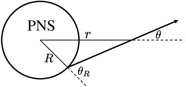
We begin our discussions with the setup employed in Ref. Sarikas et al. (2012c), in which neutrinos are emitted semi-isotropically, i.e., generated uniformly in the outward hemisphere, from each point on the neutrino sphere in the supernova core (see Fig. 1). They assumed spherical symmetry for the matter distribution and worked in the two-flavor oscillation scheme between electron-type and other types (collectively denoted by $x$ in the following) of neutrinos, which we will follow here. Then the flavor state of neutrinos can be conveniently described by $2\times 2$ density matrices $\mathbf{\Phi}_{E,u}$, in which the diagonal components represent the fluxes of individual flavors of neutrinos that have an energy $E$ and propagate in a direction specified by $u$; $u$ is defined as $u\equiv\sin^{2}\theta_{R}$ with the emission angle $\theta_{R}$ measured from the radial direction on the neutrino sphere of a radius $R$; that off-diagonal components express the transitions from one flavor to another.

The time evolutions of the density matrices are described by the von Neumann equations:

$$i\partial_{r}\mathbf{\Phi}_{E,u}=[\mathbf{H}_{E,u},\mathbf{\Phi}_{E,u}],$$ (1)

where the Hamiltonian matrices are expressed as

$$\mathbf{H}_{E,u,r}= \left(\dfrac{\mathbf{M}^{2}}{2E}+\sqrt{2}G_{F}\mathbf{N}_{l}\right)\dfrac{1}{v_{u}}$$

$$+\dfrac{\sqrt{2}G_{F}}{4\pi r^{2}}\int_{-\infty}^{\infty}dE^{\prime}\int_{0}^{1}du^{\prime}\left(\dfrac{1}{v_{u^{\prime}}v_{u}}-1\right)\mathbf{\Phi}_{E^{\prime},u^{\prime}}.$$ (2)

In the above equations, $\mathbf{M}^{2}$ is the mass-square matrix, which describes the vacuum oscillation; the diagonal matrix $\mathbf{N}_{l}=\mathrm{diag}(n_{e}-n_{e^{+}},0)$ expressed with the number densities of electron $n_{e}$ and positron $n_{e^{+}}$ represents the matter-induced MSW oscillation; it is tacitly assumed here that other charged leptons do not exist in the supernova core; $r$ is the distance from the center of proto neutron star (PNS) and $v_{u}=\cos\theta=\sqrt{1-uR^{2}/r^{2}}$ corresponds to the radial velocity of neutrino. Note that these equations are nonlinear actually, since the Hamiltonians include $\mathbf{\Phi}$’s themselves (the last term in Eq. (2)).

We then recast $\mathbf{\Phi}_{\omega,u}$ into

$$\mathbf{\Phi}_{\omega,u}=\dfrac{\mathrm{Tr}\mathbf{\Phi}_{\omega,u}}{2}I+\dfrac{F_{\omega,u}^{e}-F_{\omega,u}^{x}}{2}\begin{pmatrix}s_{\omega,u}&S_{\omega,u}\\ S_{\omega,u}^{*}&-s_{\omega,u}\end{pmatrix},$$ (3)

where $F_{\omega,u}^{e}$ and $F_{\omega,u}^{x}$ are the fluxes of $\nu_{e}$ and $\nu_{x}$ at the neutrino sphere, respectively, and we use $\omega\equiv\varDelta m^{2}/2E$ instead of $E$ to specify the energy of neutrino just for later convenience. As mentioned above, it is the non-vanishing off-diagonal components $S_{\omega,u}$ that indicate the flavor oscillations. They are small compared with the diagonal components at the beginning of the conversion, since neutrinos are produced in one of the flavor eigenstates initially. This fact is the basis of the linear analysis in the following sections.

II.2 Linear Stability Condition

As mentioned just now, since neutrinos are produced in one of the flavor eigenstates, which corresponds to $s_{\omega,u}=1$ and $S_{\omega,u}=0$ or a diagonal form of $\bm{\Phi}_{E,u}$ in Eq. (3), one can assume in the initial phase of the flavor oscillation that the off-diagonal component $S$ of $\mathbf{\Phi}$ is still small and can be treated linearly. This is the idea here. Note that the flavor eigenstate is a fixed point of Eq. (1) if one ignores a small off-diagonal component of $\mathbf{M}^{2}$ and the flavor conversion can be regarded as the instability of this fixed point. Assuming $|S|\ll 1$ and $s=1$, we obtain the linearized equation for $S$ from Eq. (1) as follows:

$$i\partial_{r}S_{\omega,u}= (\omega+u\bar{\lambda})S_{\omega,u}$$

$$-\mu\int_{0}^{1}du^{\prime}\int_{-\infty}^{\infty}d\omega^{\prime}(u+u^{\prime})g_{\omega^{\prime},u^{\prime}}S_{\omega^{\prime},u^{\prime}},$$ (4)

in which $g_{\omega,u}$ is the energy spectrum of neutrino and $\lambda=\sqrt{2}G_{F}[n_{e}(r)-n_{\bar{e}}(r)](R^{2}/2r^{2})$ and $\mu=\{\sqrt{2}G_{F}[F_{\bar{\nu}_{e}}(R)-F_{\bar{\nu}_{x}}(R)]/4\pi r^{2}\}(R^{2}/2r^{2})$ correspond to the potentials produced by matter and neutrinos, respectively, and $\bar{\lambda}$ is defined as $\bar{\lambda}\equiv\lambda+\epsilon\mu$. Note that the energy spectrum $g$ is normalized as $\int_{-\infty}^{0}d\omega\int_{0}^{1}dug_{\omega,u}=-1$ and hence $\epsilon\equiv\int_{-\infty}^{\infty}d\omega\int_{0}^{1}dug_{\omega,u}$ represents the asymmetry between neutrino and anti-neutrino.

Considering short-wavelength perturbations, we assume a following form of solutions:

$$S_{\omega,u}=Q_{\omega,u}e^{-i\Omega r}.$$ (5)

This is nothing but a (local) normal mode analysis in the spatial regime. It is valid as long as the wavelength $\sim$ ($1/\Omega$) is much shorter than the typical length scale in the background configuration. Inserting Eq. (5) into Eq. (4), we obtain eigenvalue equations as

$$(\omega+u\bar{\lambda}-\Omega)Q_{\omega,u}=\mu\int_{0}^{1}du^{\prime}\int_{-\infty}^{\infty}d\omega^{\prime}(u+u^{\prime})g_{\omega^{\prime},u^{\prime}}Q_{\omega^{\prime},u^{\prime}}.$$ (6)

These integral equations have non-trivial solutions for $Q$ only when $\Omega$ takes one of the eigenvalues. If the eigenvalue has a positive imaginary part, the corresponding $S$ will grow exponentially with $r$ at least locally, which implies that the fixed point is linearly unstable. Since the eigenvalue equations are real, the eigenvalues are either real numbers or pairs of complex numbers that are conjugate to each other. It follows then that if there is a non-real eigenvalue, it immediately means instability.

Equation (6) can be solved as follows. Since the right hand side of Eq. (6) is just linear in $u$, $Q_{\omega,u}$ should be expressed as

$$Q_{\omega,u}=\dfrac{a+bu}{\omega+u\bar{\lambda}-\Omega},$$ (7)

with $a$ and $b$ being constants to be determined. Putting this back into Eq. (6), we obtain the following homogeneous linear equations for the constants:

$$\begin{pmatrix}I_{1}-1&I_{2}\\ I_{0}&I_{1}-1\end{pmatrix}\begin{pmatrix}a\\ b\end{pmatrix}=0.$$ (8)

The elements of the matrix in the above equations are given as the following integrals:

$$I_{n}\equiv\mu\int_{0}^{1}du\int_{-\infty}^{\infty}d\omega\dfrac{u^{n}g_{\omega,u}}{\omega+u\overline{\lambda}-\Omega}.$$ (9)

Finally we obtain the equation to determine the eigenvalue $\Omega$ from the condition that Eq. (8) should have non-trivial solutions:

$$D(\Omega)\equiv(I_{1}-1)^{2}-I_{0}I_{2}=0.$$ (10)

III Spurious Modes

III.1 Discretization of the Eigenvalue Equations

We now demonstrate that spurious modes appear when the eigenvalue equations (6) are solved approximately by discretizing $Q$ as follows:

$$(\omega_{k}+u_{c}\bar{\lambda}-\Omega)Q_{k,c}=\mu\sum_{i=1}^{N_{\omega}}\sum_{b=1}^{N_{a}}\varDelta\omega\varDelta u(u_{c}+u_{b})g_{i,b}Q_{i,b}.$$ (11)

Here the integrals in the original equations are replaced with finite summations, in which $N_{\omega}$ and $N_{a}$ are the numbers of the bins in the energy- and angle-distributions of neutrinos. Equation (11) is ($N_{\omega}\times N_{a}$) dimensional, homogeneous, linear equations, which give non-trivial solutions to $Q$ when $\Omega$ takes appropriate values, which are nothing but the eigenvalues of the matrix derived from Eq. (11):

$$M_{kc,ib}=(\omega_{k}+u_{c}\bar{\lambda})\delta_{ki}\delta_{cb}-\mu\varDelta\omega\varDelta u(u_{c}+u_{b})g_{i,b}.$$ (12)

Then $Q$’s are the corresponding eigenvectors.

One may solve Eq. (10) instead by evaluating the integrals in $I_{n}$ numerically. This can be done also by discretizing the integrand and replacing the integrals with finite sums as

$$I_{n}=\mu\sum_{i=1}^{N_{\omega}}\sum_{b=1}^{N_{a}}\varDelta\omega\varDelta u\dfrac{u_{b}^{n}g_{i,b}}{\omega_{i}+u_{b}\overline{\lambda}-\Omega}.$$ (13)

We note that the two methods are essentially the same because they are both obtained by approximating the distribution function $g_{\omega,u}$ as

$$g_{\omega,u}=\sum_{i=1}^{N_{\omega}}\sum_{b=1}^{N_{a}}g_{\omega_{i},u_{b}}\varDelta\omega\varDelta u\delta(\omega-\omega_{i})\delta(u-u_{b}).$$ (14)

The same eigenvalues and eigenvectors are hence obtained in both approaches. What is important here is that all of these supposedly approximate solutions do not actually correspond to the real solutions of the original equations. This is understood from the fact that the number of the solutions for the former depends on the number of bins employed. The solutions of Eq. (11) that do not correspond to any real modes are called spurious modes.

III.2 Characteristics of Spurious Modes

We elucidate the features of the spurious modes, using a simple model with a monochromatic energy distribution Sarikas et al. (2012c):

$$g_{\omega,u}=\left[(1+\epsilon)\delta(\omega-\omega_{0})-\delta(\omega+\omega_{0})\right]B(u).$$ (15)

In this expression, $B(u)$ is an angular distribution and is assumed in this section to be

$$B(u)=1,$$ (16)

which corresponds to the semi-isotropic emission from the neutrino sphere. For this neutrino distribution in the background, we can perform the integrals in $I_{n}$ analytically as

$$I_{n}(\Omega)=\dfrac{\mu}{\bar{\lambda}}\left[(1+\epsilon)\left\{U_{+}^{n}\ln\left(1-\dfrac{1}{U_{+}}\right)+\sum_{j=0}^{n-1}\dfrac{1}{n-j}U_{+}^{j}\right\}\right.$$

$$\left.-\left\{U_{-}^{n}\ln\left(1-\dfrac{1}{U_{-}}\right)+\sum_{j=0}^{n-1}\dfrac{1}{n-j}U_{-}^{j}\right\}\right],$$ (17)

where we define

$$U_{+}(\Omega)\equiv\dfrac{\Omega-\omega_{0}}{\overline{\lambda}},\ \ U_{-}(\Omega)\equiv\dfrac{\Omega+\omega_{0}}{\overline{\lambda}}.$$ (18)

Then Eq. (10) can be solved numerically to a desired accuracy without difficulties. We hence regard the modes so obtained as true modes and use them as reference in the following.

Figure 2: The imaginary part of $\Omega$, $\mathrm{Im}\Omega$, as a function of $\mu$ for the exact (red dashed lines) and approximate (blue solid lines) solutions for different numbers of angular bins. From top to bottom the numbers of bins $N_{a}$ are 1, 2, 4 and 8. We employ $B(u)=1$ for these calculations. Note that only the leftmost branch of the approximate solutions (blue solid lines) approaches the true solutions (red dashed lines) as $N_{a}$ increases and is regarded as the (approximate) physical solution whereas all the other approximate solutions are spurious, moving rightwards away from the true solutions as $N_{a}$ increases.

Figure 3: Absolute values of $D(\Omega)$ on the complex plain of $\Omega$. The integrals in $I_{n}$ are performed analytically. The plus indicates one of the complex zero points of $D(\Omega)$. The gray line is the branch cut of $D(\Omega)$ on the Riemann surface. Note that only one of the zero points approaches the true one as $N_{a}$ increases.

Figure 4: Same as Fig. 3 except that the integrals are approximately evaluated with the discretization. The numbers of angular bins $N_{a}$ are $1$, $2$, $4$ and $8$ clockwise from top left. Plus signs indicate some of the zero points of $D(\Omega)$ whereas orange dots correspond to the exact root of $D(\Omega)$ given in Fig. 3.

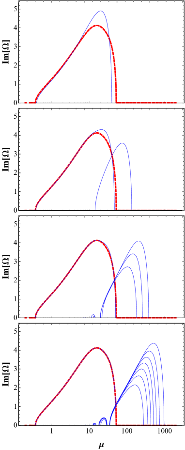
We find that Eq. (10) has 2 solutions or eigenvalues $\Omega$ for $\epsilon=0.5$ and $\lambda=0$. They are either both real or complex conjugate to each other, depending on the value of $\mu$. See the dashed line in Fig. 2, in which we show the imaginary parts of the true and approximate solutions as a function of $\mu$. Note that they are by definition non-vanishing only of the complex solutions, for which we present only those solutions with positive imaginary parts, since others are complex conjugate to them. One can see that there is a range of $\mu$, $\sim 0.4<\mu<\sim 50$, in which the true eigenvalue acquires a non-vanishing imaginary part. On the other hand, the discretized equations (Eq. (11)) with $N_{a}$ angular bins yield $2N_{a}$ eigenvalues (solid lines in Fig. 2). It is clear that only one of these solutions approximate the true solution, which is indeed corroborated in the figure by the fact that it comes closer to the true solution as the number of angular bins is increased. This is not the case of other solutions, on the other hand. In fact, they have different ranges of $\mu$, where they become complex and have non-vanishing $\mathrm{Im}\Omega$’s, and those regions move away from the true one in general as we deploy more angular bins. They are the spurious modes we are concerned with in this paper. Their characteristics mentioned above are not our original findings but just the reproduction of what were presented in Sarikas et al. (2012c). We show them here again because we will begin our analysis with these simple solutions.

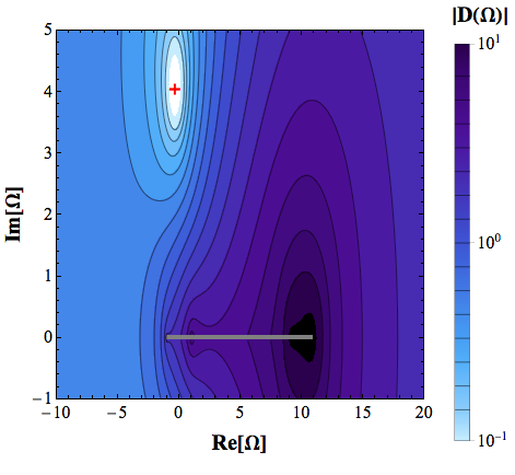
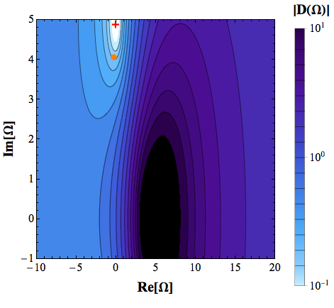
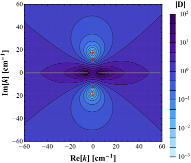
The inspection of $D(\Omega)$ gives us the hint of the reason why the spurious modes are produced by the discretization. Figure 3 exhibits in the complex $\Omega$ plane the absolute values of $D(\Omega)$ obtained from the analytical integrations of $I_{n}$ (Eq. (17)) whereas Fig. 4 displays the same quantities but for $I_{n}$ evaluated approximately with the discretization (Eq. (13)). When exactly calculated, $D(\Omega)$ has a branch cut from $-\omega_{0}$ to $\omega_{0}+\bar{\lambda}$ on the real axis in the Riemann surface. There is a discontinuity in the imaginary part of $D(\Omega)$ on this cut. In fact, it has the same absolute value but has opposite signs just above ($\mathrm{Im}\Omega>0$) and below ($\mathrm{Im}\Omega<0$) the cut. Note that in Fig. 3 the cut is indicated with a gray line although $|D(\Omega)|$ is continuous. In Fig. 4, on the other hand, not the branch cut but poles appear on and near the line, at which the cut should be located, and $D(\Omega)$ is analytic except on these poles. This feature is unchanged and only the number of poles increases if we deploy larger numbers of bins.

This situation can be demonstrated more explicitly in equations. When we evaluate the integrals in $I_{n}$ by the discretization, they are expressed as

$$I_{n}=\mu\sum_{b=1}^{N_{a}}u_{b}^{n}B(u_{b})\left(\dfrac{1+\epsilon}{\omega_{0}+u_{b}\overline{\lambda}-\Omega}-\dfrac{1}{-\omega_{0}+u_{b}\overline{\lambda}-\Omega}\right).$$ (19)

These are sums of fractional functions of $\Omega$, the poles of which are $\omega_{0}+u_{b}\bar{\lambda}$ and $-\omega_{0}+u_{b}\bar{\lambda}$. This difference in the singularity structures in $D(\Omega)$ is responsible for the appearance of the spurious modes. This may be understood as follows. When we search for the roots of $D(\Omega)$, we first combine the fractions in $I_{n}$ to a single fraction with the common denominator and then seek for the roots of the numerator, which is a polynomial in $\Omega$. Its degree becomes larger as the number of bins is increased. As a result, one obtains more roots inevitable. It should be now apparent that the point here is that the branch cut is replaced with the poles by the discretization of $g_{\omega,\mu}$ in Eq. (14). This leads in fact to $D(\Omega)$ that never approaches the true one even if one increases the number of bins as long as it is finite. It was argued in Sarikas et al. (2012c) that if one deploys a large enough number of bins, the range of $\mu$, where the spurious modes develop non-vanishing imaginary parts, may not overlap with those for the true modes and the spurious modes become harmless. As can be seen in Fig. 2, however, the behavior of the spurious modes is not simple: the range strongly depends on the number of bins; it happens in fact that all the spurious modes become real in the $\mu$-range of interest at some $N_{a}$ but the imaginary part becomes non-vanishing again at larger $N_{a}$. The problem is hence that we simply do not know a priori what number of $N_{a}$ is appropriate.

IV Analytical-Integration Approach

IV.1 Polynomial Approximation

The approximate evaluation of the integrals $I_{n}$ with the discretization of the distribution function generates the poles instead of the branch cut in $D(\Omega)$ and is the ultimate culprit for the spurious roots of $D(\Omega)$. It is hence a natural expectation that we can avoid the spurious modes if the integrals in $I_{n}$ are approximated in such a way that no poles would be generated. A simple way to do this is to approximate the distribution function $g_{\omega,u}$ not with the delta function but with a polynomial. Here we continue to assume for simplicity that the neutrino distribution is monochromatic and $g_{\omega,u}$ is expressed as in Eq. (15). $B(u)$, on the other hand, is an arbitrary continuous function.

Let us suppose that $B(u)$ is approximated as a polynomial of $d$-th degree:

$$B(u)=\sum_{k=0}^{d}b_{k}u^{k}.$$ (20)

Then, using the following formula

$$\int_{0}^{1}du\dfrac{u^{n}}{u-x}=x^{n}\ln\left(1-\dfrac{1}{x}\right)+\sum_{j=0}^{n-1}\dfrac{1}{n-j}x^{j},$$ (21)

we can perform the integrals in $I_{n}$ analytically to obtain

$$I_{n}(\Omega)= \dfrac{\mu}{\bar{\lambda}}\sum_{k=0}^{d}b_{k}\biggl{[}\biggl{\{}(1+\epsilon)U_{+}^{k+n}\ln\left(1-\dfrac{1}{U_{+}}\right)$$

$$+\sum_{j=0}^{k+n-1}\dfrac{1}{k+n-j}U_{+}^{j}\biggr{\}}-\biggl{\{}U_{-}^{k+n}\ln\left(1-\dfrac{1}{U_{-}}\right)$$

$$+\sum_{j=0}^{k+n-1}\dfrac{1}{k+n-j}U_{-}^{j}\biggr{\}}\biggr{]}.$$

Here and henceforth, the summation is defined to be zero when the upper limit is smaller than the lower limit; the logarithmic function $\ln(z)$ should take the principal value. It is apparent that in this approximation, $I_{n}$ consists of polynomial or logarithmic functions of $\Omega$, which have no pole.

Figure 5: The original function (red line) and the polynomial approximations (blue lines) of $B(u)$ (top panel) and the absolute values of the differences between them (bottom panel). The dotted, dot-dashed, short dashed, long dashed and solid lines correspond, respectively, to the polynomial degrees $d$ of $0$, $1$, $2$, $3$ and $4$.

Figure 6: Top: the imaginary part of $\Omega$ as a function of $\mu$ for the solutions of Eq. (10) with $I_{n}$ given in Eq. (LABEL:Iintegrated). The line styles denote the polynomial degrees $d$ as in Fig. 5. Bottom: the absolute values of the differences between the exact and approximate solutions for $d=4$.

Figure 7: The absolute values of $D(\Omega)$ on the complex plain of $\Omega$ for $B(u)$ given in Fig. 5 with $\mu=20$. The degree of the polynomial is set to $d=1$ and 4 in the top and bottom panels, respectively.

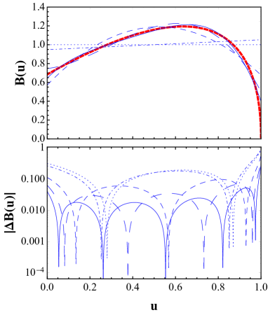
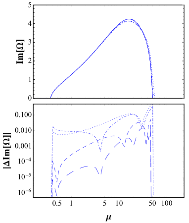
We now demonstrate that this method works as expected indeed. We employ a simple angular distribution adopted in Ref. Mirizzi and Serpico (2012b). $B(u)=(N_{\bar{\nu}_{e}}U_{\bar{\nu}_{e}}(u)+N_{\bar{\nu}_{x}}U_{\bar{\nu}_{x}}(u))/(N_{\bar{\nu}_{e}}-N_{\bar{\nu}_{x}})$ with $N_{\bar{\nu}_{e}}=1$, $N_{\bar{\nu}_{x}}=0.62$, $U_{\bar{\nu}_{e}}(u)=(3/2)(1-u)^{1/2}$ and $U_{\bar{\nu}_{x}}(u)=2(1-u)$; $\epsilon$ is set to 0.5. Note that the ratio of $N_{\nu_{e}}$ to $N_{\nu_{x}}$ is the same as that of $N_{\bar{\nu}_{e}}$ to $N_{\bar{\nu}_{x}}$ in this setup: $N_{\nu_{e}}:N_{\bar{\nu}_{e}}:N_{\nu_{x}}:N_{\bar{\nu}_{x}}=1.5:1:0.93:0.62$. This $B(u)$ is approximated with a polynomial function, which is determined by minimizing the integrated square of errors from the original function. We show in Fig. 5 both the original function and the polynomial approximations of $B(u)$ as well as the errors. As the degree of the polynomials increases, the approximation gets better just as expected. We then solve Eq. (10) with Eq. (LABEL:Iintegrated). The results are shown Fig. 6. It is obvious that no spurious mode is produced in this approach and the approximate solutions converge to the supposedly exact one as the degree of polynomial is increased and $B(u)$ is better approximated. The absence of the spurious modes is also corroborated in Fig. 7, in which we present the absolute values of $D(\Omega)$ obtained approximately in this method. It is clear that there is only one zero point.

It is evident from Eq. (LABEL:Iintegrated) that the polynomial approximation generates a branch cut in the Riemann surface along the real axis from $\Omega=-\omega_{0}$ to $\omega_{0}+\bar{\lambda}$, the same feature as for the exact $D(\Omega)$. The important thing in avoiding the spurious mode are the fact that the integrals in $I_{n}$ can be done analytically and that the original features of the Riemann surface are maintained by the approximation for $g_{\omega,u}$. The use of the polynomial functions is hence not essential and any functions will be fine as long as they satisfy these conditions. For example, one may use not only $u^{n}$ but also $u^{n}\sqrt{1-u^{2}}$ to expand $B(u)$. In fact, it is easily confirmed that the integrals can be done still analytically and the essential feature of the Riemann surface is retained also in this case. We have confirmed that no spurious mode appears then.

The choice of base functions should depend on the distribution function. It is certainly better if the distribution function is approximated accurately by a smaller number of the base functions. Note that if the approximation is not accurate, it may happen that a new spurious eigenvalue appears and/or a true eigenvalue disappears. It is important in this context to point out that the number of true modes is related with that of the "crossings" in the distribution function Banerjee et al. (2011), i.e., the neutrino oscillation tends to be triggered when the energy or angular distribution changes sign. We should hence approximate the distribution function so that the number of "crossings" should be unchanged.

IV.2 Piecewise Constant Approximation

In the previous section we approximated the angular distribution of neutrino as a whole. We stressed particularly the importance of retaining the essential feature of the Riemann surface in the approximation. This may be relaxed, though. As a matter of fact, we demonstrate in this section that a piecewise constant approximation to the angular distribution is sufficient to avoid the spurious modes. This approximation will be of practical use in dealing with numerical data, which are normally provided only at discrete grid points. We divide the interval $[0,1]$ into $N_{a}$ sub-intervals, $\{[s_{b-1},s_{b}]\}\ (b=1,2,\cdots,N_{a},\ s_{0}=0,\ s_{N_{a}}=1)$, and the function $u^{n}B(u)$ in the integrand of $I_{n}$ is approximated as a constant $u_{b}^{n}B(u_{b})$ in each interval with $u_{b}\equiv(s_{b-1}+s_{b})/2$. Then the integrals can be performed analytically for each interval and the results are given as

$$I_{n}(\Omega)= \mu\sum_{b=1}^{N_{a}}\int_{s_{b-1}}^{s_{b}}duu_{b}^{n}B(u_{b})$$

$$\times\biggl{(}\dfrac{1+\epsilon}{\omega_{0}+u\bar{\lambda}-\Omega} -\dfrac{1}{-\omega_{0}+u\bar{\lambda}-\Omega}\biggr{)}$$

$$= \dfrac{\mu}{\bar{\lambda}}\sum_{b=1}^{N_{a}}u_{b}^{n}B(u_{b})\biggl{[}(1+\epsilon) \ln\dfrac{\omega_{0}+s_{i}\bar{\lambda}-\Omega}{\omega_{0}+s_{i-1}\bar{\lambda}-\Omega}$$

$$-\ln \dfrac{-\omega_{0}+s_{i}\bar{\lambda}-\Omega}{-\omega_{0}+s_{i-1}\bar{\lambda}-\Omega}\biggr{]}$$ (23)

We have confirmed that Eq. (10) with this representation of $I_{n}$ do not produce spurious modes. Note that the essential feature of the Riemann surface is changed in this case. In fact, there is still the same branch cut along the real axis but it is actually a union of sub-cuts from $\Omega=\pm\omega_{0}+s_{i-1}\bar{\lambda}$ to $\Omega=\pm\omega_{0}+s_{i}\bar{\lambda}$ and the branching singularities occur at both ends of each sub-cut. In spite of this change in the Riemann surface, the spurious modes do not appear.

One may think that the piecewise constant approximation considered here is equivalent to the discretization, which was responsible for the generation of the spurious mode. This is not the case, however. The point is that we have exactly performed the integrals in $I_{n}$ in each sub-interval for the constant angular distribution whereas in the discretization approximation the integrals are evaluated approximately by sampling at a finite number of points $u_{i}$ (see Eq. (11)). In the latter case, even if the eigenvector $Q_{\omega,u}$ diverges at $u\in[0,1]\backslash\{u_{i}\}$, the approximated integrals are not affected and remain finite although they would diverge if the integrals were done exactly for such $Q_{\omega,u}$. They cannot be an eigenvector in the piecewise constant approximation, either, since the integrals are divergent. Note also that the discontinuities at the boundaries of the sub-intervals are responsible for the appearances of the extra branching points in the piecewise constant approximation; they pose no serious problem, though, since the integrals approach the true values as the number of intervals increases; this is in sharp contrast to the discretization approach.

One should be reminded that the accuracy still matters in the piecewise constant approximation. Indeed a new spurious mode may appear and/or a true mode may disappear if the approximation is not very good. One may hence need to deploy many sub-intervals. One may well consider to use a piecewise linear (or higher-order) approximation instead of the piecewise constant one. After all, how many sub-intervals or what base functions should be used depends on the distribution function at hand. What is important regardless, however, is that the problem with the spurious modes arising from the discretization of the distribution is resolved in principle in the polynomial or piecewise constant approximation.

IV.3 Multi-Energies

So far we have dealt with a monochromatic distribution. In reality, however, neutrinos have continuous energy spectra. Then the $\omega$ integration in $I_{n}$ becomes non-trivial. One may think that it is necessary to approximate $g_{\omega,u}$ so that the double integrals in $I_{n}$ could be done analytically and should not change the structure of the Riemann surface. Fortunately, this is not so difficult as it sounds.

What we need to respect most is to retain the essential feature of the Riemann surface. One way to do this may be to change the integral variable $\omega$ to $p\equiv\omega+u\bar{\lambda}$ as

$$I_{n}=\mu\int_{-\infty}^{\infty}dp\dfrac{G_{n}(p)}{p-\Omega}$$ (24)

with

$$G_{n}(p)\equiv\int_{0}^{1}duu^{n}g_{p-u\bar{\lambda},u}.$$ (25)

The latter function $G_{n}(p)$ can be evaluated by the discretization of the integrand in $u$. We can then approximate it with a polynomial function and perform the integral in Eq. (24) analytically just as in the previous sections.

There are some complications in this method, though. Since the integral range extends to infinity, the integral would be divergent if $G_{n}(p)$ were approximated with polynomial functions nominally. In reality, $G_{n}(p)$ goes to 0 as $|p|\to\infty$ and the integrals are convergent. This suggests that $G_{n}(p)$ should be approximated with functions that ensure the convergence of the integrals. It is normally difficult to perform the integrals analytically for such kinds of functions, however, and even if it can be done, the results tend to be complicated. From a practical point of view, we had better truncate the integral at range $p_{\mathrm{min}}$ and $p_{\mathrm{max}}$. Then the branch cut in the Riemann surface is shrunk to the line connecting $p_{\mathrm{min}}$ and $p_{\mathrm{max}}+\bar{\lambda}$ on the real axis although it is the entire real axis in the exact case. This may not be so serious a problem, though, since it will affect only those modes with very small imaginary parts.

The piecewise approximation discussed in section IV B will be also available in the present case. As a matter of a fact, $G_{n}(p)$ often looks like a Fermi-Dirac distribution and the polynomial approximation over the whole interval is not appropriate.

The method given above may not be suitable after all for the analysis of numerical data, which provide the values of $g_{\omega,u}$ only at discrete points $\{(\omega_{i},u_{b})\}$, since it is then difficult to obtain $G_{n}(p)$ at desirable points of $p$. Fortunately, we have another (and simpler indeed) option to avoid the spurious modes. In this method we approximate $g_{\omega,u}$ polynomially in $u$ for a discrete set of $\omega$ just as in the monochromatic case and then simply take the sum. This is equivalent to approximate $g_{\omega,u}$ as

$$g_{\omega,u}\simeq\sum_{i=1}^{N_{\omega}}\varDelta\omega\delta(\omega-\omega_{i})\sum_{k=0}^{d}b_{i,k}u^{k}.$$ (26)

Then the integrals in $I_{n}$ can be performed to obtain

$$I_{n}(\Omega)=\dfrac{\mu}{\overline{\lambda}}\sum_{i=1}^{N_{\omega}}\sum_{k=0}^{d}\varDelta\omega\ b_{i,k}\biggl{\{}U_{i}^{k+n}\ln\left(1-\dfrac{1}{U_{i}}\right)$$

$$+\sum_{j=0}^{k+n-1}\dfrac{1}{k+n-j}U_{i}^{j}\biggr{\}},$$ (27)

where $U_{i}$’s are defined as

$$U_{i}(\Omega)\equiv\dfrac{\Omega-\omega_{i}}{\overline{\lambda}}.$$ (28)

Note that the branch cut is again shrunken to a finite interval $[\omega_{1},\omega_{N_{\omega}}+\bar{\lambda}]$ on the real axis and there occurs many branching singularities on the cut. It turns out that this is sufficient to avoid the spurious modes.

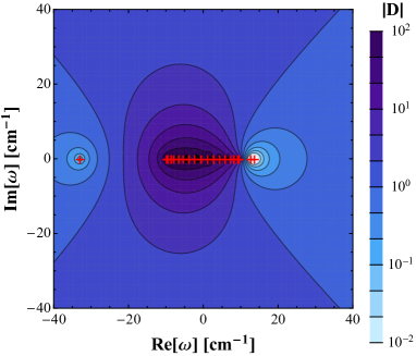
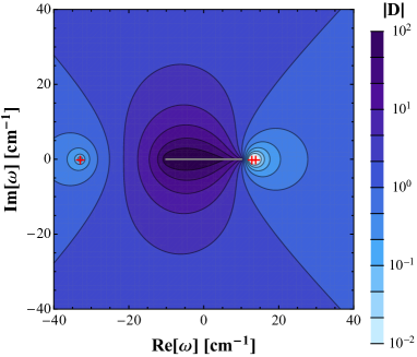
Figure 8 presents an example. We show the behavior of $|D(\Omega)|$ for a simple multi-energy and multi-angle distribution employed in Ref. Mirizzi and Serpico (2012b):

$$g_{\omega,u}= \dfrac{\varDelta m^{2}}{2\omega^{2}}[\theta(\omega)\{F_{\nu_{e}}(E(\omega),u)-F_{\nu_{x}}(E(\omega),u)\}$$

$$+\theta(-\omega)\{F_{\bar{\nu}_{e}}(E(\omega),u)-F_{\bar{\nu}_{x}}(E(\omega),u)\}]$$ (29)

with

$$F_{\nu_{\alpha}}=N_{\nu_{\alpha}}\times\varphi_{\nu_{\alpha}}(E)\times\tilde{U}_{\nu_{\alpha}}(u),$$ (30)

$$\varphi_{\nu_{\alpha}}(E) =\dfrac{(1+\alpha)^{1+\alpha}}{\Gamma(1+\alpha)}\dfrac{E^{\alpha}}{\left\langle E_{\nu}\right\rangle^{\alpha+1}}\exp\left[-\dfrac{(1+\alpha)E}{\left\langle E_{\nu}\right\rangle}\right]$$ (31)

and

$$\tilde{U}_{\nu_{\alpha}}(u) =\left(\dfrac{\beta_{\alpha}}{2}+1\right)(1-u)^{\beta_{\alpha}/2}.$$ (32)

Here we set the model parameters as follows: $(\left\langle E_{\nu_{e}}\right\rangle,\left\langle E_{\bar{\nu}_{e}}\right\rangle,\left\langle E_{\nu_{x}}\right\rangle)=(12,15,18)\mathrm{MeV}$, $N_{\nu_{e}}:N_{\bar{\nu}_{e}}:N_{\nu_{x}}=1.5:1:0.62$, $\beta_{e}=1,\beta_{x}=3$, $\Delta m^{2}=10$, $\lambda=0$ and $\mu=1$. Zero points are marked with red pluses in the figure. In the top panel, we give the result for the discretization approximation. It is apparent that a lot of spurious modes appear on the real axis. On the other hand, there is no such spurious mode in the middle and the bottom panels, in which $I_{n}$ is evaluated with Eqs. (24) and (27), respectively. We remark that the energy integrals are truncated at $\omega\approx\pm 2$ and, as a result, the branch cut runs approximately from $\sim-2$ to $\sim 3$, which is indicated again by the gray lines in the figure.

Figure 8: Absolute values of $D(\Omega)$ on the complex plain of $\Omega$ for the simple multi-energy and multi-angle model given in the text. $D$ is evaluated in the discretization approximation with $N_{\omega}=16,N_{a}=2$ (top panel) or calculated in Eq. (24) with 16 sub-intervals in energy and with $G_{n}(p)$ being evaluated in Eq. (25) with 16 angular bins (middle panel) or obtained with Eq. (27) for $N_{\omega}=32,d=4$ (bottom panel). Zero points are marked with red pluses and the branch cuts are indicated with the gray lines.

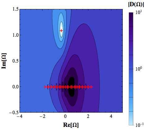
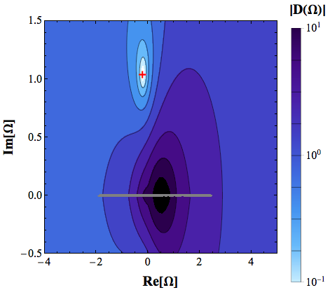
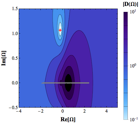
V Applications to the Dispersion Relation Approach

V.1 Linear Analysis in the Dispersion Relation Approach

More recently, Izaguirre et al. Izaguirre et al. (2017) proposed an elegant approach to the linear analysis of the collective neutrino oscillation based on the "dispersion relation". In their approach, not only the instability in the spatial regime but also in the temporal regime can be handled on the same basis. In this section we demonstrate that the method proposed in this paper can be applied also to this dispersion relation approach.

We begin with a brief review of the dispersion relation approach. The equations of motion for free-streaming neutrinos without collisions but with flavor conversions are written as Sigl and Raffelt (1993); Cardall (2008)

$$(\partial_{t}+\bm{v}\cdot\bm{\nabla}_{\bm{r}})\rho=i[\rho,H],$$ (33)

where the Hamiltonian is given as

$$H=\dfrac{M^{2}}{2E}+v^{\mu}\Lambda_{\mu}\dfrac{\sigma_{3}}{2}+\sqrt{2}G_{F}\int d\Gamma^{\prime}v^{\mu}v_{\mu}^{\prime}\rho^{\prime}.$$ (34)

In these equations $\rho(t,\mathbf{r},\mathbf{p})$ is again the density matrix, $(v^{\mu})=(1,\bm{v})$ is the neutrino four velocity and $\Lambda^{\mu}$ consists of $\Lambda^{0}=\sqrt{2}G_{F}(n_{e}-n_{\bar{e}})$ and the corresponding current $\bm{\Lambda}$. One can recognize the similarity of the above equation to Eq. (1), in which only time-independent oscillations are considered for radially-moving neutrinos.

We decompose $\rho$ as

$$\rho=\dfrac{f_{\nu_{e}}+f_{\nu_{x}}}{2}+\dfrac{f_{\nu_{e}}-f_{\nu_{x}}}{2}\begin{pmatrix}s&S\\ S^{*}&-s\end{pmatrix}$$ (35)

with the maximum occupation numbers $f_{\nu_{e}}$ and $f_{\nu_{x}}$ just as in Eq. (3). Then, $s=1$ and $S=0$ corresponds to flavor eigenstates, which are fixed points of the equations of motion if one ignores the minor off-diagonal elements in the mass matrix in vacuum. Linearizing Eq. (33) in the neighborhood of one of these fixed points, we obtain the equation for $S$ as

$$i(\partial_{t}+\bm{v}\cdot\bm{\nabla}_{\bm{r}})S_{\bm{v}}=v^{\mu}(\Lambda_{\mu}+\Phi_{\mu})S_{\bm{v}}-\int\dfrac{d\bm{v}^{\prime}}{4\pi}v^{\mu}v_{\mu}^{\prime}G_{\bm{v^{\prime}}}S_{\bm{v^{\prime}}},$$ (36)

where we define $G_{\bm{v}}$ and $\Phi^{\mu}$ as

$$G_{\bm{v}}=\sqrt{2}G_{F}\int_{0}^{\infty}\dfrac{dEE^{2}}{2\pi^{2}}\left[f_{\nu_{e}}(E,\bm{v})-f_{\bar{\nu}_{e}}(E,\bm{v})\right]$$ (37)

and

$$\Phi^{\mu}\equiv \int\dfrac{d\bm{v}}{4\pi}G_{\bm{v}}v^{\mu}.$$ (38)

Assuming the following form of solution in the local approximation, $S_{\bm{v}}=Q_{\bm{v}}e^{-i(\Omega t-\bm{K}\cdot\bm{r})}$ we obtain again the homogeneous integral equation for $Q_{\bm{v}}$ as follows:

$$v^{\mu}k_{\mu}Q_{\bm{v}}=-\int\dfrac{d\bm{v}^{\prime}}{4\pi}v^{\mu}v_{\mu}^{\prime}G_{\bm{v}^{\prime}}Q_{\bm{v}^{\prime}},$$ (39)

where we introduce $k^{\mu}=(\omega,\bm{k})=K^{\mu}-\Lambda^{\mu}-\Phi^{\mu}$. Since the right hand side of this equation is expressed as $v^{\mu}a_{\mu}$ with

$$a^{\mu}\equiv-\int\dfrac{d\bm{v}}{4\pi}v^{\mu}G_{\bm{v}}Q_{\bm{v}},$$ (40)

we can write $Q_{\bm{v}}$ as $Q_{\bm{v}}=v^{\mu}a_{\mu}/v^{\mu}k_{\mu}$. Substituting this back into Eq. (39), we obtain the equation for $a^{\mu}$ as

$$\Pi^{\mu\nu}(\omega,\bm{k})a_{\nu}=0,$$ (41)

in which $\Pi^{\mu\nu}$ is given as

$$\Pi^{\rho\sigma} =\eta^{\rho\sigma}+\int\dfrac{d\bm{v}}{4\pi}G_{\bm{v}}\dfrac{v^{\rho}v^{\sigma}}{\omega-\bm{v}\cdot\bm{k}}$$

$$=\eta^{\rho\sigma}+\int_{-1}^{1}d\mu\dfrac{1}{\omega-k\mu}G^{\rho\sigma}(\mu)$$ (42)

with

$$G^{\rho\sigma}(\mu)\equiv\int_{0}^{2\pi}\dfrac{d\phi}{4\pi}G_{\bm{v}}v^{\rho}v^{\sigma}.$$ (43)

In these equations, $\mu$ is the cosine of the zenith angle $\theta$ and $\phi$ is the azimuthal angle in the polar coordinates, which are chosen so that the zenith should be oriented in the direction of $\bm{k}$. Then the following condition has to be satisfied:

$$D(\omega,\bm{k})\equiv\det\Pi=0,$$ (44)

which finally gives us the dispersion relation (DR) between $\omega$ and $\bm{k}$. It should be noted that the integral in Eq. (42) has a quite similar structure to those in $I_{n}$ given in Eq. (9), the fact that is eventually responsible for the appearance of the spurious modes also in this approach.

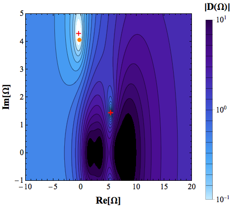
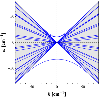
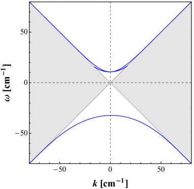
In the DR approach we first search for solutions of Eq. (44), in which $\omega$ and $k$ are both real. They normally form several branches. If there opens a gap in $\omega$ among these branches, that is, there is no solution with real $k$ for the range of real $\omega$, then $k$ should be complex and an instability occurs in the spatial regime. If, on the other hand, a gap opens in $k$, an instability in the temporal regime should occur. The DR approach is hence very convenient to judge in which regime the instability occurs (see also Ref. Capozzi et al. (2017)). Note, however, that we still need to solve Eq. (44) somehow to obtain complex solutions and the spurious modes also obtain if one were to solve Eq. (44) either to obtain $\omega$ for a given $k$ or to find $k=|\bm{k}|$ for a given $\omega$ and the direction of $\bm{k}$ by discretizing the angular distribution $G_{\bm{v}}$. This can be inferred from the similarity of the integral in Eq. (42) to those in $I_{n}$. Fig. 9 shows the DR obtained by the discretization method with 4 angular bins for a toy model with $G_{\bm{v}}\propto(\mu+1)\mu(\mu-0.65)$. Note that this distribution is axisymmetric with respect to $\bm{k}$. Such distributions are expected only for $\bm{k}$ parallel to the radial direction in spherically symmetric background. Otherwise, i.e., either for a non-radial $\bm{k}$ or in non-spherical background, $G_{\bm{v}}$ should have a $\phi$-dependence in general. Even in that case the present method works just as well Morinaga et al. . In this figure the negative $k$ corresponds to the mode going in the opposite direction and $\mu$ is replaced with $-\mu$ in $G_{\bm{v}}$. In this toy model, DR consists of many branches, only three of which are true modes and the rest are spurious. It is important that all spurious branches lie in the so-called zone of avoidance Izaguirre et al. (2017), in which $\omega=ck$ is satisfied for $|c|\leq 1$ and the integral in Eq. (42) diverges. This fact also explains why the spurious modes occur in the discretization method. If the integral in Eq. (42) is conducted approximately by the discretization, then the integrand is evaluated only at a finite number of points and the integral does not diverge even for combinations of $\omega$ and $k$ in the zone of avoidance unless one of the sampling points accidentally coincides with $k$/$\omega$. The zone of avoidance is hence useful to judge which branch is spurious at a glance.

Figure 9: The dispersion relation for a toy model with $G_{\bm{v}}\propto(\mu+1)\mu(\mu-0.65)$. The top panel displays the results obtained by the discretization of the $\mu$ integrals with 4 angular bins while in the bottom panel we present the results of the analytical-integration method. The shaded regions are the zone of avoidance.

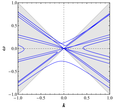
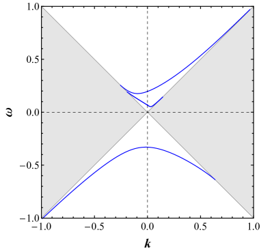
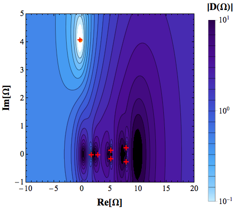
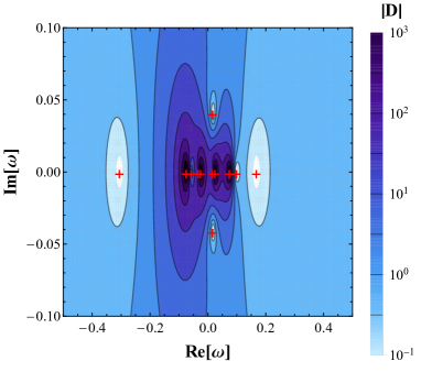
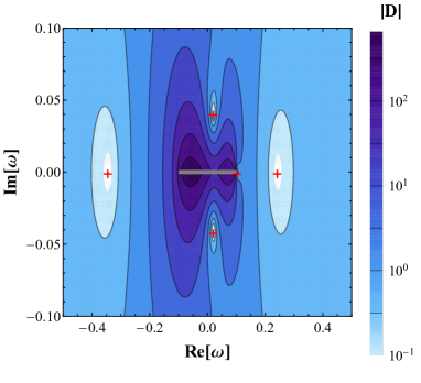
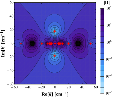
The complex solutions are more involved. In fact, judging from the gap in $\omega$ for the three true branches, one may think that there will be instabilities only in the spatial regime. This is not true, however. In fact, we show in Fig. 10 the absolute values of $D(\omega,\bm{k})$ in the complex $\omega$ plain for $k=0.1$. In the upper panel, where the results of the discretization approximation are shown, there are many real spurious modes and only outer three modes ($\omega\approx-0.3$, 0.1 and 0.15) are true modes as mentioned above (see also Fig. 9). What is more important here is the fact that there exist complex true modes also (see the lower panel of Fig. 10), which cannot be recognized from DR alone. We hence have to search for complex solutions of Eq. (44) somehow and again face the same problem of the spurious modes.

Figure 10: The Absolute values of $D(\omega,\bm{k})$ in the complex plane of $\omega$ for $k=0.1$. The angular distribution $G_{\bm{v}}$ is the same as in Fig. 9. The top panel displays the results obtained by the discretization of the $\mu$ integrals with 4 angular bins while in the bottom panel we present the results of the analytical-integration method. Red pluses mark the positions of the zero points of $D$ in each method. The gray line in the bottom panel indicates the branch cut of the Riemann surface obtained in the analytical-integration method.

V.2 Analytical-Integration Approach

Figure 11: The Absolute values of $D(\omega,\bm{k})$ in the complex plane of $k$ for $\omega=0.4$ for a toy model with $G_{\bm{v}}\propto-(\mu+0.5)(\mu-1)$. The top panel displays the results obtained by the discretization of the $\mu$ integrals with 20 angular bins while in the bottom panel we present the results of the analytical-integration method. Red pluses mark the positions of the zero points of $D$ in each method. The gray lines in the bottom panel indicate the branch cuts of the Riemann surface obtained in the analytical-integration method.

Figure 12: The dispersion relation obtained in the analytical-integration method for the same toy model as in Fig. 11. The shaded regions are the zone of avoidance.

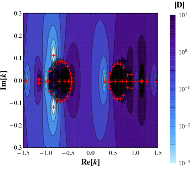
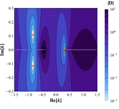
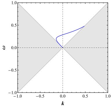
Although there was no complex spurious modes in the previous model, this is not the case in general. In fact, we show in the upper panel of Fig. 11 the complex spurious solutions obtained for the case of $G_{\bm{v}}\propto-(\mu+0.5)(\mu-1)$ in the discretization method with 20 angular bins. The corresponding DR is presented in Fig. 12. These spurious modes can be avoided by approximating $G(\mu)$ polynomially again. Then we can evaluate the remaining integrals with respect to the energy $E$ and the azimuthal angle $\phi$ just by discretization, since they do not yield poles of $\omega$ or $k$.

The concrete procedure is the following: each component of $G^{\rho\sigma}(\mu)$ is first approximated as

$$G^{\rho\sigma}(\mu)\simeq\sum_{i=0}^{d}g_{i}^{\rho\sigma}\mu^{i};$$ (45)

then the integrals in $\Pi$ are performed analytically as

$$\int_{-1}^{1}d\mu\dfrac{1}{\omega-k\mu}G^{\rho\sigma}(\mu)$$

$$\simeq\sum_{i=0}^{d}g_{i}^{\rho\sigma}\int_{-1}^{1}d\mu\dfrac{\mu^{i}}{\omega-k\mu}$$

$$=\dfrac{1}{k}\sum_{i=0}^{d}g_{i}^{\rho\sigma}\biggl{[}\left(\dfrac{\omega}{k}\right)^{i}\ln\dfrac{\omega+k}{\omega-k}-\sum_{m=1}^{\left\lceil\frac{i}{2}\right\rceil}\dfrac{2}{2m-1}\left(\dfrac{\omega}{k}\right)^{i-2m+1}\biggr{]};$$ (46)

finally the determinant of $\Pi$ is calculated and its zero points are looked for either in the complex plane of $\omega$ for a given $k$ or in the complex plane of $k$ for a given $\omega$. Note that in both cases $D(\omega,\bm{k})$ has a branch cut in the Riemann surface of $\omega$ or $k$ on the parts of the real axis that satisfy $|\omega|\leq|k|$ for each $k$ or $\omega$. We show in the bottom panel of Fig. 10 the absolute values of $D(\omega,\bm{k})$ in the complex $\omega$ plane obtained in this way. The value of $k$ is set to 0.1. It is evident that the spurious modes are all gone and only the true modes, three real and two complex ones, are remaining. In the bottom panel of Fig. 11, in which an example that has complex spurious modes is exhibited, we demonstrate that our method can also eradicate these complex spurious modes successfully. The reason should be now clear: the essential feature in the Riemann surface is maintained in the analytical-integration approach.

VI Applications to Simulation Data

As mentioned earlier, we have in mind the applications of our method to more realistic data provided by numerical simulations. Then the neutrino distribution functions available are discrete in energy and angles from the beginning. It is hence the purpose of this section to demonstrate that such discrete data can be handled without any difficulty by our method.

Figure 13: The angular distributions of $\nu_{e}$ (green pluses) and $\bar{\nu}_{e}$ (red crosses) at the time of 200 ms post bounce and at the radius of 40 km obtained in a SN simulation. The blue points are the difference between them and the blue solid line is the polynomial approximation to it.

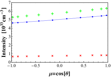
Here we employ the neutrino distributions obtained in a spherically symmetric simulation of core collapse supernovae Nagakura . The progenitor is a non-rotating massive star of $11.2M_{\odot}$ Woosley et al. (2002). The dynamics of core collapse, bounce and shock stagnation is computed with a Boltzmann-radiation-hydrodynamics code, for details of which we refer readers to Nagakura et al. (2014, 2017a): it solves hydrodynamics equations and Boltzmann equations for neutrino transport simultaneously; Newtonian self-gravity is implemented; a realistic equation of state based on the relativistic mean field theory for uniform nuclear matter is adopted Nagakura . This model fails to produce an explosion as is normally the case in spherically symmetric simulations. The neutrino distribution functions we use here are taken from the snapshot at the post-bounce time of 200ms. The radial position is $r=40\mathrm{km}$.

The angular distributions of neutrinos that we employ are shown in Fig. 13. We note that it is the difference between the intensities of $\nu_{e}$ and $\bar{\nu_{e}}$ that is most important for the collective flavor oscillation as is understood from Eq. (37). Figures 14 and 15 show the DR and absolute values of $D$, respectively, in which the upper panels are obtained by discretization whereas the lower ones are the results of the analytical-integration method. From the former it is apparent that many spurious modes appear when we evaluate the integral in Eq. (42) by discretization. In sharp contrast the analytical-integration method generate none of them. In this case, the gap opens in $\omega$, implying a possible instability in the spatial regime (see Fig. 16). It is also confirmed with no difficulty in our method that there is no unstable mode in the temporal regime for, e.g., $k=10\mathrm{cm}$ as demonstrated in the bottom panel of Fig. 15.

Figure 14: Dispersion relations for the angular distribution in Fig. 13. The top panel displays the results obtained by the discretization approximation while in the bottom panel we present the results of the analytical-integration method. The shaded regions are the zone of avoidance.

Figure 15: The Absolute values of $D(\omega,\bm{k})$ in the complex plane of $\omega$ for $k=10\mathrm{cm}^{-1}$ for the angular distribution given in Fig. 13. The top panel displays the results obtained by the discretization approximation while in the bottom panel we present the results of the analytical-integration method. Red pluses mark the positions of the zero points of $D$ in each method. The gray line in the bottom panel indicates the branch cut of the Riemann surface obtained in the analytical-integration method.

Figure 16: The Absolute values of $D(\omega,\bm{k})$ in the complex plane of $k$ for $\omega=5\mathrm{cm}^{-1}$ for the angular distribution given in Fig. 13. The top panel displays the results obtained by the discretization approximation while in the bottom panel we present the results of the analytical-integration method. Red pluses mark the positions of the zero points of $D$ in each method. The gray lines in the bottom panel indicate the branch cuts of the Riemann surface obtained in the analytical-integration method.

VII Conclusions

The appearance of the spurious modes is a vexing problem in the analysis of collective flavor oscillations of neutrino in the supernova core. They emerge even in the linear analysis more often than not when one solves the integro-differential equations by the ordinary discretization. In principle, they can be distinguished from the true modes, since the spurious ones do not converge to real solutions as the number of bins employed for the discretization is increased. Such procedures are inefficient, however, if one were to analyze numerical data obtained in realistic simulations systematically and, if possible, in real time. In this paper, we have analyzed in detail why the spurious modes appear in the first place and have proposed a simple method to avoid them from the beginning in the local linear analysis.

We have found that the ultimate source of the spurious modes is a generation of pole singularities in the approximate angular integrations by the discretization, in which the angular distribution of neutrino is expressed as a superposition of delta functions. The exact integration would produce two branching points and a cut in between instead. It is hence reasonable to consider that the spurious modes will not appear if one retain the singularity structure in the approximation. The easiest way to do this may be to approximate the angular distribution with polynomials and perform the angular integration analytically. We have demonstrated for some toy models that the idea really works as expected. We have started with the time-independent mode propagating in the radial direction under the background of matter distributed spherically in space and monochromatic neutrinos emitted semi-isotropically from the neutrino sphere. Note that polynomials are not the unique option but any base functions will work equally well as long as they do not change the singularity structure. We need to strike a balance then between accuracy of the approximation and easiness of the integration. We have also shown that the condition may be relaxed a bit: the single branch cut may be replaced by a union of sub-branch cuts that are produced, for example, in the piecewise constant approximation. In this case the pole singularities are replaced by branching-point singularities but no spurious mode is produced. This finding is important in applying the method to numerical data, which are normally provided only on a set of discrete grid points.

We have then considered a multi-energy case. We have observed that it is sufficient to apply the polynomial approximation or the piecewise constant approximation only to the angular integral. The remaining integral with respect to the energy can be done simply by discretization. This is understood from the fact that no pole is produced in these methods.

Our method can be also applied to the dispersion relation approach, which was proposed more recently and treats the instabilities both in the spatial and temporal regimes on the equal basis. We have shown that only the spurious modes with real $\omega$ and $k$ exist in the zone of avoidance and argued that the existence of such modes is closely related with the reason why the spurious modes appear in the first place. The spurious modes are not restricted to the zone of avoidance, though. We have demonstrated indeed that they can occur in the temporal regime even when a gap is opening in $\omega$ and a spatial instability is expected. The opposite is also possible. More importantly, we have confirmed that these spurious modes are all eliminated by our method again. This is mainly because the integro-differential equations in the dispersion relation approach have essentially the same structure as those for the time-independent modes. The point is again that the approximate evaluation of the integral should not produce pole singularities when the branching singularities are expected. We have finally applied our method to numerical data obtained in a realistic supernova simulation in spherical symmetry in space. We have observed that there occurs no spurious mode. Although only radially-propagating modes have been considered in this calculation, we believe that this is sufficient to demonstrate that our method works just as well for realistic data.

Modes with non-radial $\bm{k}$ can be also treated in our method. In that case, the azimuthal dependence of the angular distribution needs to be treated appropriately. Since we measure the zenith and azimuth angles not from the radial direction but from the direction of $\bm{k}$ in our method, the angular distribution becomes $\phi$-dependent even in the spherically symmetric background, in which it is axisymmetric with respect to the local radial direction. We can deal with this by spherical-harmonics expansions and rotations of coordinates. The details will be described in our forthcoming paper Morinaga et al. , in which we will conduct linear analysis in more general settings with the method proposed here. Note that the angular distribution function of neutrino is no longer axisymmetric if the background is not spherically symmetric, which is believed to be the case in the supernova core owing to hydrodynamical instabilities Janka et al. (2016); then we need to handle non-trivial $\phi$-dependence even for the radially-propagating modes.

In this paper, we have assumed the local approximation, which is valid in the short-wavelength limit. In general, however, we need to take into account the global background distribution. Then the eigen modes cannot be given by exponential functions any longer. It remains to be studied if our method can be extended to this global linear analysis. If the answer is affirmative, our method may be further applied to the analysis of the original nonlinear equations for the collective flavor oscillations. It will be also interesting to see how the inclusion of collision terms in linear analysis modifies the whole picture if the collective oscillations are expected to occur near the neutrino sphere in the linear analysis neglecting them. We are currently conducting linear analysis with the present method for numerical data, which have become available very recently from realistic radiation-hydrodynamics simulations of CCSNe under axisymmetry in space, in which the Boltzmann equations were solved directly for neutrino transfer Nagakura et al. (2017b). The results will be reported elsewhere Azari et al. .