Pure glueball states in a Light-Front holographic approach

Abstract

A phenomenological analysis of the scalar glueball and scalar meson spectra is carried out by using the AdS/QCD framework in the bottom-up approach. The resulting spectra are in good agreement for glueballs with lattice QCD results and for mesons with PDG data. We make use of the relation between the mode functions in AdS/QCD and the wave functions in Light-Front $QCD$ to discuss the mixing of glueballs and mesons. The results of our investigation point out that above 2 GeV scalar particles will appear in almost degenerate pairs of unmixed glueball and mesons states leading to an interesting phenomenology whereby gluon dynamics could be well investigated.

I Introduction

Glueballs have been a matter of theoretical study and experimental search since the formulation of the theory of the strong interaction Quantum Chromodynamics (QCD) Fritzsch:1973pi ; Fritzsch:1975wn , QCD sum rules  Shifman:1978bx ; Mathieu:2008me , QCD based models Mathieu:2008me and Lattice QCD computations both with sea quarks Gregory:2012hu and in the pure glue theory Morningstar:1999rf ; Chen:2005mg ; Lucini:2004my have been used to determine their spectra and properties. However, due to the lack of phenomenological support much debate has been associated with their properties Mathieu:2008me . Glueballs, if they exist, will mix with meson states of the same quantum numbers, and therefore their direct characterization is difficult to disclose.

A fruitful strategy to investigate non perturbative features of glueballs is the use of QCD models inspired by the holographic conjecture. Recently we have used these so called AdS/QCD models to study the glueball spectrum Vento:2017ice ; Rinaldi:2017wdn . The holographic principle relies in a correspondence between a five dimensional classical theory with an AdS metric and a supersymmetric conformal quantum field theory with $N_{C}\rightarrow\infty$. Since the latter is different from QCD, an approach called bottom-up is usually adopted Polchinski:2000uf ; Brodsky:2003px ; DaRold:2005mxj ; Karch:2006pv . It consists in properly modifying the five dimensional classical theory to resemble QCD as much as possible. The different models constructed in this way differ in the strategy to break conformal invariance. Since the mesons masses are $\mathcal{O}(N^{0}_{c})$ these models reproduce the essential features of the meson spectrum Erlich:2005qh ; deTeramond:2005su ; Colangelo:2008us . Two of the most widely used models are the hard-wall (HW) and the soft-wall (SW) models. The former consists in introducing an explicit cut off in the fifth coordinate z, $0\leq z\leq z_{max}=1/\Lambda_{QCD}$. However, the HW model is not able to reproduce the Regge trajectories of the mesonic spectrum. To this aim, in the SW model, a dilaton field is introduced to softly break conformal invariance. Since the glueball masses are also $\mathcal{O}(N_{C}^{0})$ these models were extended to study the glueball spectrum Rinaldi:2017wdn ; Colangelo:2007pt ; Capossoli:2015ywa . Keeping in mind the relation between AdS/QCD models and the $1/N_{C}$ expansion of QCD other observables of $\mathcal{O}(N_{C}^{0})$ have been investigated. In fact, since in the the planar limit ($N_{C}\rightarrow\infty$) hadrons are stable and non-interacting, these AdS/QCD models are appropriate to evaluate structure functions and spectra. For example form factors (ffs), parton distribution functions (PDFs), generalized parton distribution functions and transverse dependents PDFs have been calculated with reasonable agreement with the data Brodsky:2006uqa ; Abidin:2009hr ; Chakrabarti:2013dda ; Rinaldi:2017roc ; Bacchetta:2017vzh ; deTeramond:2018ecg . All these analyses were inspired by the investigation on hard deep inelastic scattering at small $x$ within AdS/QCD Polchinski:2002jw . In addition, $\mathcal{O}(1/N_{C}^{2})$ observables like the pomeron contribution to proton-proton scattering Domokos:2009hm ; Shuryak:2013sra and the elastic cross section Watanabe:2018owy have been also described with holographic inspired models.

Following our investigations on the scalar glueball spectrum, we discuss in what follows some phenomenological consequences by comparing theoretical results with data. The experimentally determined scalar ”mesons” with spin parities $J^{PC}=0^{++}$ are known as the $f_{0}$ mesons Patrignani:2016xqp . Our aim is to describe the glueball lattice spectrum by means of the AdS/QCD correspondence and to compare it with the spectrum of $f_{0}$’s. Only when the masses of the glueballs and the $f_{0}$’s are close mixing is to be expected Vento:2004xx . However, if the masses are close, but the dynamics generating the resonance states is different, mixing will not happen Vento:2015yja . Therefore, we are looking for meson and glueball states with similar masses but generated by different dynamics. These scalar particles will appear in the phenomenological spectrum as mostly glueball or mostly meson.

We use for our analysis the bottom-up approach of the AdS/QCD correspondence Polchinski:2000uf ; Brodsky:2003px ; DaRold:2005mxj . This approach describes glueball and meson dynamics in a very transparent fashion Erlich:2005qh ; Karch:2006pv ; Rinaldi:2017wdn ; Colangelo:2007pt . In section II we describe the scalar glueball spectrum and the meson spectrum in several AdS/QCD approaches. In section III we will discuss glueball-meson mixing and finally in the conclusions we extract some consequences of our analysis.

II Scalar glueball and scalar meson spectrum in a bottom-up approach

The botton-up approach on the AdS/CFT correspondence starts from QCD and attempts to construct its five-dimensional holographic dual. One implements duality in nearly conformal conditions defining QCD on the four dimensional boundary and introducing a bulk space which is a slice of $AdS_{5}$ whose size is related to $\Lambda_{QCD}$  Polchinski:2000uf ; Brodsky:2003px ; Erlich:2005qh ; DaRold:2005mxj .

The metric of this space can be written as

$$ds^{2}=\frac{R^{2}}{z^{2}}(dz^{2}+\eta_{\mu\nu}dx^{\mu}dx^{\nu})+R^{2}d\Omega_{5},$$ (1)

where $\eta_{\mu\nu}$ is the Minkowski metric and the size of the slice in the holographic coordinate $0<z<z_{max}$ is related to the scale of QCD, $z_{max}=\frac{1}{\Lambda_{QCD}}$. This is the so called hard wall approximation. Later on, in order to reproduce the Regge trajectories, the so called soft wall approximation was introduced  Karch:2006pv ; Capossoli:2015ywa . Within the bottom-up strategy and in the soft wall approach, glueballs arising from the correspondence of fields in $AdS_{5}$ have been studied in ref.  Colangelo:2007pt . In our recent work we have described the scalar glueball spectrum as that of a graviton in $AdS_{5}$ with a modified soft wall metric Rinaldi:2017wdn . In Fig. 1 we reproduce the results of these references for the glueball spectrum.

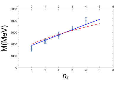
Figure 1: Glueball spectrum obtained with the soft wall model (dashed-dotted) Colangelo:2007pt and soft wall graviton model (solid) Rinaldi:2017wdn . These calculations were reported in ref.  Rinaldi:2017wdn . The lattice data are from refs.  Morningstar:1999rf ; Chen:2005mg ; Lucini:2004my as shown in Table 1. The dots label the scalar glueballs and the triangles the tensor glueballs.

In order to clarify the discussion of the present investigation let us recall the formalism to describe glueballs and mesons in AdS/QCD soft wall models.

II.1 The glueball in a soft wall model

For a scalar glueball, the dilaton the action is:

$$S=\int d^{5}x~{}\sqrt{-g}e^{-\phi(z)}\Big{[}g^{MN}\partial_{M}G~{}\partial_{N}G+M^{2}_{5g}G^{2}\Big{]}~{},$$ (2)

where here $g_{MN}$ is the metric of eq. (1), $G$ the scalar glueball field, $M^{2}_{5g}$ is the $AdS_{5}$ mass and the dilaton function is $\phi(z)=z^{2}$. In the case of scalars, the boundary operator conformal dimension $\Delta$, is related to $M_{5}$ as follows Capossoli:2015ywa :

$$\Delta=2\pm\sqrt{4+R^{2}M_{5}^{2}}~{}.$$ (3)

In the case of the scalar glueball, $\Delta=4$ thus $M_{5g}=0$. The equation of motion from eq. (2) for the glueball field reads:

$$\partial_{M}\Big{[}\sqrt{-g}e^{-\phi(z)}g^{MN}\partial_{N}G\Big{]}=0~{}.$$ (4)

The above equation can be rewritten as a Schrödinger like equation:

$$-\Psi{{}^{\prime\prime}}(z)+\Big{[}z^{2}+\frac{15}{4z^{2}}+2\Big{]}\Psi(z)=\mu^{2}\Psi(z)~{},$$ (5)

where here

$$G(z,x)=e^{iq\cdot x}\Psi(z)\left(\frac{z}{R}\right)^{3/2}e^{z^{2}/2}~{}.$$ (6)

In the above relation, $x$ is a four vector in the Minkowski space and $-q^{2}=\mu^{2}$ with $\mu$ an adimensional glueball mass. As can be seen in ref. Colangelo:2007pt the solution of eq. (5) leads to the following mode spectrum

$$\mu^{2}_{k}=4k+8,$$ (7)

where $k=0,1,2,\ldots$. The corresponding normalized mode function for mode number $k=n_{g}$ is can be written as:

$$\Psi_{n_{g}}(z)=\sqrt{(n_{g}+1)(n_{g}+2)/2}\;e^{-z^{2}/2}\;z^{5/2}\;_{1}F_{1}(-n_{g},3,z^{2})~{}.$$ (8)

II.2 The scalar meson in the soft wall model

For a scalar meson, the dilaton the action is:

$$S=\int d^{5}x~{}\sqrt{-g}e^{-\phi(z)}\Big{[}g^{MN}\partial_{M}S~{}\partial_{N}S+M^{2}_{5m}S^{2}\Big{]}~{},$$ (9)

where $S$ the scalar meson field and $M^{2}_{5m}$ is the $AdS_{5}$ mass. The conformal dimension for the scalar meson field is $\Delta=3$ thus $M^{2}_{5g}R^{2}=-3$. The equation of motion from eq. (9) for the scalar meson field reads Colangelo:2008us ,:

$$-\Psi{{}^{\prime\prime}}(z)+\Big{[}z^{2}+\frac{3}{4z^{2}}+2\Big{]}\Psi(z)=\mu^{2}\Psi(z)~{},$$ (10)

where here

$$S(z,x)=e^{iq\cdot x}\Psi(z)\left(\frac{z}{R}\right)^{3/2}e^{z^{2}/2}~{}.$$ (11)

In the above relation $-q^{2}=\mu^{2}$ with $\mu$ an adimensional scalar meson mass. The solution of this equations Colangelo:2008us leads to the following mode spectrum, by

$$m^{2}_{k}=4k+6,$$ (12)

where $k=0,1,2,\ldots$. The normalized mode function for mode number $k=n_{m}$ is

$$\Psi_{n_{m}}(z)=\sqrt{2(n_{m}+1)}\;e^{-z^{2}/2}\;z^{3/2}\;_{1}F_{1}(-n_{m},2,z^{2})~{}.$$ (13)

II.3 The soft wall graviton model

In ref. Rinaldi:2017wdn , we discussed the possibility that the glueball field is dual to a graviton. However, in order to recover the above results for the scalar meson, it is convenient to generalize the background metric to

$$\bar{g}_{MN}=e^{-\alpha^{2}z^{2}/R^{2}}g_{MN}~{},$$ (14)

with $\alpha^{2}<0$ in order to have bound states. The equation of motion is obtained by solving the Einstein equation for the above metric Rinaldi:2017wdn . Setting $R=1$ this equation reads

$$\frac{d^{2}\phi}{dz^{2}}+\left(\alpha^{2}z-\frac{3}{z}\right)\frac{d\phi}{dz}+\left(\frac{8}{z^{2}}+6\alpha^{2}+\mu^{2}+4\alpha^{2}z^{2}\right)\phi-\frac{8}{z^{2}}e^{-\alpha^{2}z^{2}}\phi=0.$$ (15)

In this case one can also obtain a Schrödinger like equation by performing the change of function

$$\phi(z)=e^{\alpha^{2}z^{2}/4}\left(\frac{z^{2}}{\alpha^{2}}\right)^{\frac{3}{2}}\Psi(z)$$ (16)

which using the adimensional variable $t=az/\sqrt{2}$ where $a=i\alpha$ becomes

$$-\Psi^{\prime\prime}(t)+\Big{[}\frac{8e^{2t^{2}}}{t^{2}}-\frac{17}{4t^{2}}+14-15t^{2}\Big{]}\Psi(t)=\frac{2\mu^{2}}{a^{2}}\Psi(t)~{},$$ (17)

The mode spectrum has no analytical solution and was obtained numerically  Rinaldi:2017wdn . We take $a=\sqrt{2},t=z$ and the equation resembles those of the other approaches with $\mu$ an adimensional glueball mass.

II.4 Phenomenological analysis

As we have just recalled the AdS/QCD models provide us with a succession of mass modes of differential equations, which in general, one has to obtain numerically. In the case of glueballs an exception is the standard soft wall model where the expression turns out to be analytic, $\mu{{}^{2}}(n_{g})=4n_{g}+8$, where $n_{g}$ is the corresponding mode number Colangelo:2007pt . In order to reach the experimental results we have to multiply the adimensional modes $\mu(n_{g})$ by an energy scale $\varepsilon$, i.e. $m^{2}(n_{g})=\varepsilon^{2}\mu^{2}(n_{g})$ To determine $\varepsilon$ we use here the technique, developed in ref. Rinaldi:2017wdn . We display the spectrum obtained by fitting one $AdS$ mode to a physical state, for example in the case of glueballs we fit the lowest mode to the lowest lying glueball and determine an initial value for $\varepsilon$. We then proceed by seeding the rest of the lattice data on the plot and by varying slightly $\varepsilon$ we get a best fit to the whole spectrum. The lattice data used are shown in Table 1  Morningstar:1999rf ; Chen:2005mg ; Lucini:2004my . We also use for the fit the results for the tensor glueball states since the theory predicts degeneracy between the scalar an the tensor glueball for the soft wall models. In Fig. 1 we show the results for all models analyzed. The best fit for the soft wall model is obtained for $\varepsilon^{\prime}=710$ MeV. The soft wall graviton model has no analytical mode solution, it is given by a numerical function $m(n_{g})=\varepsilon^{\prime\prime}f(n_{g}))$, and the shown fit is for $\varepsilon^{\prime\prime}=370$ MeV. Both models lead to a reasonable fit of the data. The difference between them arises for heavy states. The soft wall dilaton model has a quadratic behavior that softens the slope at high energies. The soft wall graviton model has an almost linear behavior showing no softening of the slope in the region analyzed.

$J^{PC}$	$0^{++}$	$2^{++}$	$0^{++}$	$2^{++}$	$0^{++}$	$0^{++}$
MP	$1730\pm 94$	$2400\pm 122$	$2670\pm 222$
YC	$1719\pm 94$	$2390\pm 124$
LTW	$1475\pm 72$	$2150\pm 104$	$2755\pm 124$	$2880\pm 164$	$3370\pm 180$	$3990\pm 277$

Table 1: Glueball masses [MeV] from lattice calculations by MP  Morningstar:1999rf , YC Chen:2005mg and LTW  Lucini:2004my .

Meson	$f_{0}(500)$	$f_{0}(980)$	$f_{0}(1370)$	$f_{0}(1500)$	$f_{0}(1710)$	$f_{0}(2020)$	$f_{0}(2100)$	$f_{0}(2200)$
PDG	$475\pm 75$	$990\pm 20$	$1350\pm 150$	$1504\pm 6$	$1723\pm 6$	$1992\pm 16$	$2101\pm 7$	$2189\pm 13$

Table 2: Scalar meson masses [MeV] from PDG Patrignani:2016xqp

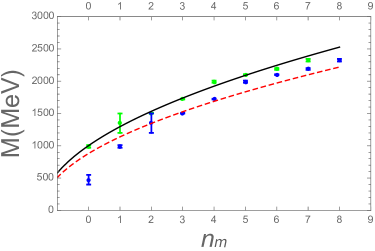
Figure 2: We plot the $f_{0}$ PDG meson spectrum Patrignani:2016xqp as a function of mode number. The lower curve considers the $f_{0}(500)$ as the lowest mass meson, while the upper curve omits this resonance and considers the $f_{0}(980)$ as the lowest mass meson. These curves arise by choosing the adequate energy scale in the meson spectrum of the soft wall model Colangelo:2008us .

In Fig. 2 we show the soft wall model fit to the PDG meson spectrum which we recall in Table 2. Many authors have argued that the $f_{0}(500)$ is not a conventional meson state but a tetraquark or a hybrid Mathieu:2008me ; Tanabashi:2018oca . The figure shows that once the $f_{0}(500)$ is taken out of the meson spectrum the soft wall model fit is excellent for $\varepsilon=410$ MeV. From now on we omit the $f_{0}(500)$ from our discussion.

Note the similarity of the scales for mesons and glueballs in the soft wall graviton model. On the contrary in the soft wall model studied despite having extremely similar equations of motion the mass scales are very different. This feature has to do with the shape of the spectra. While the meson spectrum is quadratic in the region under scrutiny, the glueball spectrum is almost linear. From this feature one may conclude that the soft wall graviton model describes well the glueball spectra.

It might surprise that the scale factors for glueballs and mesons are different. Note that we are not approximating the same theory for mesons and glueballs. Fitting the mesons with PDG data we are approximating QCD, while fitting the glueballs with lattice QCD results we are approximating Gluodynamics. However, we feel that these scales should not be vastly different, an additional reason for our liking of the soft wall graviton model. Recall that this model leads to an energy scale for glueballs of $370$ MeV and for mesons of $410$ MeV, which for the mass scales involved are very similar despite the different dynamics. Lastly, remember that our fits are $\mathcal{O}(N_{C}^{-1})$ and higher orders should be added to obtain a precise value. However, the fact that the fits are quite good suggest that the contribution of the higher order terms might be small.

In Fig. 3 we show the meson data (lower points) and the glueball lattice data (upper points). We have used to fit the meson data the soft wall model Rinaldi:2017wdn ; Colangelo:2008us . To fit the data for the glueballs we have used on the left the soft wall model  Colangelo:2007pt and on the right figure the soft wall graviton model Rinaldi:2017wdn . An interesting feature of the comparison of spectra that can be seen in Fig.3 is that the glueball masses with a certain mode number are equal to the meson masses with a larger mode number. For example, the glueball masses for $n_{g}=0,1,2$ are similar to the scalar meson masses for $n_{m}=4,7,10$ respectively. The difference in mode numbers grows as the masses of the glueballs increase due to the different slopes. Thus besides the reasonable quality of the fits, the result we would like to stress is the difference between the slopes of the glueball and meson fits for large mode numbers. The mode numbers are associated with the behavior of the mode functions. Thus, the mode function for a meson will oscillate more than that for a glueball of approximately the same mass. Therefore, despite having a similar mass the large difference in mode numbers leads one intuitively to expect that mixing will not be very strong between the heavy states. We proceed to analyze the consequences of this observation quantitatively in what follows.

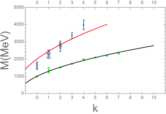
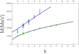
Figure 3: Left panel: fits of glueball spectrum (full upper line) and scalar meson spectrum (full lower line) obtained within the dilaton soft wall model of refs. Colangelo:2007pt ; Colangelo:2008us . The dark dots represent glueball spectrum obtained within lattice QCD Morningstar:1999rf ; Chen:2005mg ; Lucini:2004my . The light dots represent the scalar meson spectrum obtained from experimental data  Patrignani:2016xqp . Right Panel: the same as in the left panel but the fits result from the soft wall graviton model of ref. Rinaldi:2017wdn .

III Glueball-Meson mixing

One of the problems in glueball phyics is the fact that glueball candidates always appear strongly mixed with mesons states Mathieu:2008me ; Vento:2015yja . Mixing usually occurs if two states have similar masses and the same quantum numbers. Thus the scalar glueballs might mix with scalar mesons. The study of the $f_{0}$ spectrum from this perspective has led to the result that if glueballs exist, and there is no reason for its non-existence, either the $f_{0}(1500)$ or the $f_{0}(1710)$ might have a large glueball component (see Mathieu:2008me ; Vento:2015yja and references therein). Our aim here is not to contribute to this discussion, but in view of the structure of the spectra, to look for dynamical regions were mixing is not favorable and therefore states with mostly gluonic valence structure might exist. The presence of almost pure glueball states and the study of their decays would help in understanding many properties of QCD related to the physics of gluons.

In order to proceed with the discussion let us consider the holographic light-front representation of the equation of motion, in $AdS$ space. The latter can be recast in the form of a light-front Hamiltonian Brodsky:2003px

$$H_{LC}|\Psi_{k}>=M_{k}^{2}|\Psi_{k}>.$$ (18)

where $k$ represents the mode number of the corresponding particle. In the AdS/QCD light-front framework the above relation becomes a Schrödinger type equation

$$\left(-\frac{d^{2}}{dz^{2}}+V(z)\right)\Psi(z)=M_{k}^{2}\Psi(z)$$ (19)

where $z$ and $M_{k}^{2}$ in this equation are adimensional. The holographic light-front wave function are defined by $\Psi_{k}(z)=\;<z|\Psi_{k}>$ and are normalized as

$$<\Psi_{k}|\Psi_{k}>=\int dz|\Psi_{k}(z)|^{2}=1$$ (20)

The eigenmodes of Eq.(19) determine the mass spectrum. In order to fit the spectrum dimensional constants have to be introduced, e.g. the $\varepsilon$’s of previous section, which might be different for glueballs and mesons. These dimensional constants do not affect the adimensional variables and therefore do not affect the properties of the properly normalized wave functions. Thus the mode functions describe properties like probability distributions independently of those scales in terms of the adimensional variables as seen in Eq.(20).

Let us discuss mixing in a two dimensional Hilbert space generated by a meson and a glueball states, {$|\Psi_{m}>,|\Phi_{g}>$}. Mixing occurs when the hamiltonian is not diagonal in the subspace. Let us recall the discussion of two state mixing. For notational simplicity we use a linear hamiltonian model. A matrix representation of the hamiltonian in a two dimensional meson-glueball subspace is given by

$$[H]=\left(\begin{array}[]{cc}m_{1}&\beta\\ \beta&m_{2}\end{array}\right),$$ (21)

where $\beta=<\Psi_{m}|H|\Phi_{g}>$, $m_{1}=<\Psi_{m}|H|\Psi_{m}>$ and $m_{2}=<\Phi_{g}|H|\Phi_{g}>$. We are assuming $m_{2}>m_{1}$ and for simplicity $\alpha$ real and positive. Large $N_{C}$ QCD tells us that $m_{1},m_{2}\sim\mathcal{O}(N_{C}^{0})$ and $\beta\sim~{}\mathcal{O}(N_{C}^{-1/2})$ Goity:2016ty ; Vento:2004xx . After diagonalization the eigenstates have a mass

$$M_{\pm}=m\pm\sqrt{\beta^{2}+(\Delta m)^{2}},$$ (22)

where $m=(m_{1}+m_{2})/2$ and $\Delta m=(m_{2}-m_{1})/2$ and its wave functions are proportional to

$$\sim\left(\begin{array}[]{c}M_{\pm}-m_{2}\\ \beta\\ \end{array}\right)$$

Thus in the starting base the physical meson, which we assume to be the lightest of the two eigenvectors, has a wave function given by

$$|\Psi_{phy}>=\frac{1}{\sqrt{\beta^{2}+(M_{-}-m_{2})^{2}}}\;((M_{-}-m_{2})|\Psi_{m}>+\beta|\Phi_{g}>).$$ (23)

In our fit we have fixed the meson spectrum to the experimental values and therefore $|\Psi_{phy}>$ represents a physical meson state. On the other hand we have fixed the glueball spectrum to the lattice values, i.e., to the spectrum of pure gluodynamics, therefore the glueball state is our initial state $|\Phi_{g}>$, thus

$$|<\Psi_{phy}|\Phi_{g}>|^{2}=\frac{\beta^{2}}{(M_{-}-m_{2})^{2}+\beta^{2}}.$$ (24)

We conclude that the mixing probability is proportional to the overlap probability of these two wave functions.

Despite the large $N_{c}$ analysis previously presented one might suspect that for $N_{c}=3$, the overlap probability might not be as small as required to produce small $\beta$ values. The value of $\beta$ certainly depends on the modes it connects. For the lower modes it has been estimated in the linearized form of Eq.(21) to be $\beta\sim 40$ MeV Giacosa:2004ug , while the meson and glueball masses are at the level of $\sim 2000$ MeV. The heavier meson-glueball states have smaller overlap factors, as we next show, and larger masses. Therefore the $\beta$ values will be even smaller.

In the case of the standard soft wall dilaton model, the overlap factor is defined as

Figure 4: We plot the glueball for mode number $n_{g}=2$ (solid) and the meson for mode number $n=10$ (dashed). The figure on the left corresponds to the soft wall dilaton model while the figure on the right to the soft wall graviton model.

$$<\Psi_{n_{m}}|\Phi_{n_{g}}>=<G|M>=\sqrt{2(n_{m}+1)(n_{g}+1)(n_{g}+2)}\int_{0}^{\infty}dze^{-z^{2}}z^{4}\;_{1}F_{1}(-n_{g},3,z^{2})\;_{1}F_{1}(-n_{m},2,z^{2}),$$ (25)

and the overlap probability for no mixing $P_{GM}=1-|<G|M>|^{2}$. For the soft wall graviton model the overlap factor must be obtained numerically.

Figure 5: We plot the probability of no mixing for the glueball with mode numbers $n_{g}=0$ (solid),$1$ (dashed), $2$ (dotted), $3$ (dot-dashed), $4$ (solid) as a function of meson mode number $n_{m}$. The left figure is for the soft wall dilaton model while the right figure is for the soft wall graviton model.

We would like to show that meson and glueball wave functions whose mode numbers are very different, despite having almost equal masses, lead to small overlap probabilities and therefore to small mixing. To do so let us an example. We choose a glueball of mode number $n_{g}=2$ and a meson of mode number $n_{m}=10$. They can be considered as candidates for mixing because, using in the soft wall model Eqs. (7,12), the glueball mass $m(k=2)\sim 2840$ MeV and the meson mass $m(k=10)\sim 2781$ MeV. Thus this example can be considered as a prototype for a mixing scenario for heavy particles. In Fig.4 we show the mode functions for the $n_{g}=2$ glueball mode and that for the $n_{m}=10$ meson mode for both the soft wall and soft wall graviton models. The figure shows the big difference between the glueball modes in both the soft wall and soft wall graviton models. The extension of the glueball mode in the soft wall graviton model is determined by the exponential in the potential and therefore all modes die at $z\sim 2$ irrespective of their mode number. In the case of the soft wall model the extension is governed by the mode number. This difference in structure implies that in the soft wall graviton model the overlap factor is oscillating and extends over many modes even reaching large meson mode numbers $n$, while in the dilaton model only a few modes close to $n_{g}$ are contributing to the overlap as shown in Fig. 5.

Looking at Figs. 3 and 5, the favorable mixing scenario is mostly excluded in the case of heavy glueballs and mesons, since the mass condition is satisfied for very different mode numbers. For example $n_{g}=2,3,4$ the favorable meson modes of almost equal masses occur for $n_{m}\sim 10,13,17$ in the soft wall model . As can be seen in Fig. 5 this condition reduces the overlap probability for mixing dramatically. In the soft wall model the overlap probability is extremely small for the required mode number differences, while in the soft wall graviton model it oscillates at the level of maximum $10\%$ percent overlap probabilities. The outcome of our analysis is that the AdS/QCD approach predicts the existence of almost pure glueball states in the scalar sector in the mass range above $2$ GeV. The no mixing scenario is experimentally very appealing. It predicts the existence of pairs of almost degenerate states with very different decay properties. The pure glueball decays to mesons are Zweig forbidden, i.e. small widths and an increase in the proportion of strange mesons to non-strange mesons Mathieu:2008me ; Klempt:2007cp ; Crede:2008vw ; Ochs:2013gi . On the contrary the pure meson states will have a large width since they have a lot of phase space for decaying and larger decay rates to non-strange mesons than to strange mesons.

IV Conclusion

We have performed a phenomenological analysis of the scalar glueball and scalar meson spectrum based on the AdS/QCD correspondence within the soft wall dilaton and soft wall graviton approaches. Theoretical outcomes have been compared with lattice $QCD$ data in the case of the glueballs and the experimental $f_{0}$ spectrum of the PDG tables in the case of the mesons. We have noted that the slope of the glueball spectrum as a function of mode number is bigger that that of the meson spectrum in both approaches and therefore for heavy almost degenerate glueball and meson states, their mode numbers differ considerably. Assuming a light-front quantum mechanical description of AdS/QCD correspondence we have shown that the overlap probability of heavy glueballs to heavy mesons is small and thus one expects little mixing in the high mass sector. Therefore, this is the kinematical region to look for almost pure glueball states. The scenario is phenomenologically very appealing because it implies the existence of pairs of almost degenerate states with very different decay properties.

References

- (1) H. Fritzsch, M. Gell-Mann and H. Leutwyler, Phys. Lett. 47B (1973) 365.
- (2) H. Fritzsch and P. Minkowski, Phys. Lett. 56B (1975) 69.
- (3) M. A. Shifman, A. I. Vainshtein and V. I. Zakharov, Nucl. Phys. B 147 (1979) 385. doi:10.1016/0550-3213(79)90022-1
- (4) V. Mathieu, N. Kochelev and V. Vento, Int. J. Mod. Phys. E 18 (2009) 1 [arXiv:0810.4453 [hep-ph]].
- (5) E. Gregory, A. Irving, B. Lucini, C. McNeile, A. Rago, C. Richards and E. Rinaldi, JHEP 1210 (2012) 170 [arXiv:1208.1858 [hep-lat]].
- (6) C. J. Morningstar and M. J. Peardon, Phys. Rev. D 60 (1999) 034509 [hep-lat/9901004].
- (7) Y. Chen, A. Alexandru, S. J. Dong, T. Draper, I. Horvath, F. X. Lee, K. F. Liu and N. Mathur et al., Phys. Rev. D 73 (2006) 014516 [hep-lat/0510074].
- (8) B. Lucini, M. Teper and U. Wenger, JHEP 0406 (2004) 012 doi:10.1088/1126-6708/2004/06/012 [hep-lat/0404008].
- (9) V. Vento, Eur. Phys. J. A 53 (2017) no.9, 185 doi:10.1140/epja/i2017-12378-2 [arXiv:1706.06811 [hep-ph]].
- (10) M. Rinaldi and V. Vento, doi:10.1140/epja/i2018-12600-9 arXiv:1710.09225 [hep-ph],arXiv:1712.06936 [hep-ph]..
- (11) J. Polchinski and M. J. Strassler, hep-th/0003136.
- (12) S. J. Brodsky and G. F. de Teramond, Phys. Lett. B 582 (2004) 211 [hep-th/0310227].
- (13) L. Da Rold and A. Pomarol, Nucl. Phys. B 721 (2005) 79 [hep-ph/0501218].
- (14) A. Karch, E. Katz, D. T. Son and M. A. Stephanov, Phys. Rev. D 74 (2006) 015005 [hep-ph/0602229].
- (15) J. Erlich, E. Katz, D. T. Son and M. A. Stephanov, Phys. Rev. Lett. 95 (2005) 261602 [hep-ph/0501128].
- (16) G. F. de Teramond and S. J. Brodsky, Phys. Rev. Lett. 94, 201601 (2005).
- (17) P. Colangelo, F. De Fazio, F. Giannuzzi, F. Jugeau and S. Nicotri, Phys. Rev. D 78 (2008) 055009 doi:10.1103/PhysRevD.78.055009 [arXiv:0807.1054 [hep-ph]].
- (18) J. L. Goity, “Introduction to large N QCD,” XIIth Quark Confinement and the Hadron Spectrum, (Thessaloniki, Greece 2016).
- (19) P. Colangelo, F. De Fazio, F. Jugeau and S. Nicotri, Phys. Lett. B 652 (2007) 73 [hep-ph/0703316].
- (20) E. Folco Capossoli and H. Boschi-Filho, Phys. Lett. B 753, 419 (2016)
- (21) S. J. Brodsky and G. F. de Teramond, Phys. Rev. Lett. 96, 201601 (2006) doi:10.1103/PhysRevLett.96.201601 [hep-ph/0602252].
- (22) Z. Abidin and C. E. Carlson, Phys. Rev. D 79, 115003 (2009).
- (23) D. Chakrabarti and C. Mondal, Eur. Phys. J. C 73, 2671 (2013).
- (24) M. Rinaldi, Phys. Lett. B 771, 563 (2017).
- (25) A. Bacchetta, S. Cotogno and B. Pasquini, arXiv:1703.07669 [hep-ph].
- (26) G. F. de Teramond et al. [HLFHS Collaboration], Phys. Rev. Lett. 120, no. 18, 182001 (2018)
- (27) J. Polchinski and M. J. Strassler, JHEP 0305, 012 (2003).
- (28) S. K. Domokos, J. A. Harvey and N. Mann, Phys. Rev. D 80, 126015 (2009) doi:10.1103/PhysRevD.80.126015 [arXiv:0907.1084 [hep-ph]].
- (29) E. Shuryak and I. Zahed, Phys. Rev. D 89, no. 9, 094001 (2014)
- (30) A. Watanabe and M. Huang, Phys. Lett. B 788, 256 (2019)
- (31) C. Patrignani et al. [Particle Data Group], Chin. Phys. C 40 (2016) no.10, 100001. doi:10.1088/1674-1137/40/10/100001
- (32) V. Vento, Phys. Rev. D 73 (2006) 054006 doi:10.1103/PhysRevD.73.054006 [hep-ph/0401218]. Vento:2004xx
- (33) V. Vento, Eur. Phys. J. A 52 (2016) no.1, 1 doi:10.1140/epja/i2016-16001-x [arXiv:1505.05355 [hep-ph]].
- (34) M. Tanabashi et al. [Particle Data Group], Phys. Rev. D 98 (2018) no.3, 030001. doi:10.1103/PhysRevD.98.030001
- (35) F. Giacosa, T. Gutsche and A. Faessler, Phys. Rev. C 71 (2005) 025202 doi:10.1103/PhysRevC.71.025202 [hep-ph/0408085].
- (36) E. Klempt and A. Zaitsev, Phys. Rept. 454 (2007) 1 doi:10.1016/j.physrep.2007.07.006 [arXiv:0708.4016 [hep-ph]].
- (37) V. Crede and C. A. Meyer, Prog. Part. Nucl. Phys. 63 (2009) 74 doi:10.1016/j.ppnp.2009.03.001 [arXiv:0812.0600 [hep-ex]].
- (38) W. Ochs, J. Phys. G 40 (2013) 043001 doi:10.1088/0954-3899/40/4/043001 [arXiv:1301.5183 [hep-ph]].