CRISTIANI et al
*E. Cristiani, IAC–CNR, Via dei Taurini, 19 – 00185, Rome, Italy.
Comparing comparisons between vehicular traffic states in microscopic and macroscopic first-order models
Abstract
[Summary] In this paper we deal with the analysis of the solutions of traffic flow models at multiple scales, both in the case of a single road and of road networks. We are especially interested in measuring the distance between traffic states (as they result from the mathematical modeling) and investigating whether these distances are somehow preserved passing from the microscopic to the macroscopic scale. By means of both theoretical and numerical investigations, we show that, on a single road, the notion of Wasserstein distance fully catches the human perception of distance independently of the scale, while in the case of networks it partially loses its nice properties.
keywords:
LWR model, Follow-the-Leader model, traffic flow, many-particle limit, networks, multi-path model, Wasserstein distance, earth mover’s distance1 Introduction
In this paper we deal with the analysis of the solutions of traffic flow models at multiple scales. More precisely, we are interested in measuring the distance between traffic states (as they result from the mathematical modeling) and investigating whether these distances are somehow preserved passing from the microscopic to the macroscopic scale. We will consider both the case of a single road and of road networks.
Connections between microscopic (agent-based) and macroscopic (fluid-dynamics) traffic flow models are already well established. Aw et al.1, Greenberg2, and Di Francesco et al.3 investigated the many-particle limit in the framework of second-order traffic models, deriving the macroscopic ARZ4, 5 model from a particular second-order microscopic FtL6, 7 model. Instead Colombo and Rossi,8 Rossi,9 Di Francesco and Rosini,10 and Di Francesco et al.11 investigated the many-particle limit in the framework of first-order traffic models, deriving the LWR12, 13 model as the limit of a specific first-order FtL model. Let us also mention the papers by Forcadel et al.,14 Forcadel and Salazar15 which investigate the many-particle limit exploiting the link between conservation laws and Hamilton-Jacobi equations.
Moving to road networks, analogous connections are rarer. This is probably due to the fact that macroscopic traffic models on networks are in general ill-posed, since the conservation of the mass is not sufficient alone to characterize a unique solution at junctions. This ambiguity makes more difficult to find the right limit of the microscopic model, which, in turn, can be defined in different ways near the junctions. In this context let us mention the paper by Cristiani and Sahu16 which investigates the many-particle limit of a first-order FtL model suitably extended to a road network. The corresponding macroscopic model appears to be the extension of the LWR model on networks introduced by Hilliges and Weidlich17 and then extensively studied by Briani and Cristiani18 and Bretti et al.19
This paper focuses in particular on the comparison of solutions to the equations associated to first-order traffic models. It is useful to note here that many problems require the comparison of traffic states, or, in other words, the computation of the “distance” between two vehicle arrangements (at microscopic scale) or vehicle density distributions (at macroscopic scale). For example,
-
•
Theoretical study of scalar conservation laws.
-
•
Sensitivity analysis (quantifying how the uncertainty in the outputs of a model can be apportioned to different sources of uncertainty in the inputs).
-
•
Convergence of the numerical schemes (verifying that the numerical solution is close to the exact solution).
-
•
Calibration (finding the values of the parameters for the predicted outputs to be as close as possible to the observed ones).
-
•
Validation (checking if the outputs are close to the observed ones).
The question arises as to which notion of distance is the more appropriate in our context. Regarding conservation laws, which are the foundations of macroscopic models like LWR and ARZ, it is nowadays quite established that -distances are inadequate for comparing solutions, i.e. vehicular density functions, since they lead to results which can mismatch the human perception of physical distance.20 Sect. 7.1,21 For example, the -distance between two density functions and with equal total mass and disjoint supports is equal to 2, regardless how “far” the masses are. A notion of distance which instead better matches the intuition is that of Wasserstein distance (also known as -norm, earth mover’s distance, -metric, Mallows distance), which is able to quantify the effort needed to transport a certain amount of mass for a certain distance. Unfortunately, a mere application of the Wasserstein distance in a microscopic framework would only be meaningful under the assumptions that vehicles are indistinguishable and interchangeable, which of course do not hold true (ask drivers).
In this paper we study some distances between microscopic and macroscopic traffic states, which are actually usable in the context of traffic flow. Then we investigate under which assumptions they coincide and we study their behavior as the number of vehicles goes to infinity, in order to catch their scale-preserving properties.
The paper is organized as follows. In Section 2 we present the main ingredients of our investigations, i.e. the microscopic FtL model, the macroscopic LWR model, and the limit relation between the two models (on a single road and on road networks). We also recall the definition of Wasserstein distance. For all of these notions, references for numerical approximation are given. In Section 3 we introduce the definition of some distance functions particularly suitable for comparing traffic states at micro- and macro-scale. In Section 4 we investigate from the theoretical and numerical point of view the relations between the previously introduced distance functions in the case of a single road. In Section 5 we replicate the analysis of Section 4 on a road network. Finally, in Section 6 we sketch some conclusions.
2 Ingredients
2.1 Many-particle limit on a single road
Let us assume that vehicles move on a single infinite road with a single lane, and that they cannot overtake each other.
2.1.1 FtL model
Adopting a microscopic point of view, we assume that we are able to track the position of every single vehicle on the road. Moreover, we assume that the dynamics of each vehicle depend only on the vehicle itself and the vehicle in front of it, so that, in a cascade, the whole traffic flow is determined by the dynamics of the very first vehicle, termed the leader.
We denote by the number of vehicles and by their length (equal for all vehicles). We also denote by the position of (the barycenter of) the -th vehicle and we assume that at the initial time vehicles are labeled in order, i.e. . This guarantees that the -th car is just in front of the -th one. Moreover, it is assumed that at cars do not overlap, i.e. , . We are now ready to introduce the model, described by the following system of ODEs
| (1) |
where is the maximal admissible velocity and , which represents the velocity of the vehicles, is such that
| (2) |
Note that the -th vehicle is the leader and it moves at maximal velocity. In the following we will denote by the solution to (1), duly complemented with initial conditions.
Numerical approximation
System (1) will be numerically integrated by means of the explicit Euler scheme.
2.1.2 LWR model
Adopting a macroscopic point of view, we assume that we are able to track only averaged quantities like the velocity and the density (number of vehicles per length unit). Hereafter, we will assume without loss of generality that the density is normalized, i.e. corresponds to the minimal density (empty road) and corresponds to the maximal density (fully congested road).
The well known LWR12, 13 model describes the evolution of the density of vehicles by means of the following conservation law
| (3) |
Here the unknown function represents the density at time and point , while gives the velocity as a function of the density, and must be specified to complete the model. We assume that is any function such that
| (4) |
A typical simple choice often used for theoretical investigations, and that we will employ in the rest of the paper, is
| (5) |
Numerical approximation
2.1.3 Relation between scales
In order to study the many-particle limit of the FtL model described above, the number of vehicles must be no longer considered as a model parameter, rather it has to be seen as a scale parameter which goes to . From the physical point of view, the quantity which is actually preserved is the total length (or mass) of vehicles. We translate this fact by setting
| (6) |
This relation is crucial for the micro-to-macro limit since it translates the fact that the total length does not change when the number of vehicles tends to infinity, because vehicles “shrink” accordingly.
In order to recall precisely the results about the correspondence between the two models, we need to introduce first the natural spaces for the macroscopic density and for the vectors of vehicles’ positions , at any fixed time. We define
where denotes the support of any function , and
We also introduce the operators and , defined respectively as
| (7) |
and
| (8) |
where is the indicator function of any subset . The discretization operator acts on a macroscopic density , providing a vector of positions whose components partition the support of the density into segments on which has fixed integral , see Fig. 1(left). On the contrary, the operator antidiscretizes a microscopic vector of positions , giving a piecewise constant density , see Fig. 1(right).
We are now ready to state the main result about the convergence of the microscopic model (1) to the macroscopic model (3). The proof can be found in Di Francesco and Rosini10 (see also Colombo and Rossi8).
Theorem 2.1.
Remark 2.2.
2.2 Many-particle limit on networks
Let us consider the case of a road network. We define a road network as a directed graph consisting of a finite set of vertexes (junctions) and a set of oriented edges (roads) connecting the vertexes. Edges have a positive length and they are provided with a coordinate system. We assume that for each junction j , there exist disjoint subsets , representing, respectively, the incoming roads to j and the outgoing roads from j. Among junctions, we distinguish two particular subsets consisting of origins , which are the junctions j such that , and destinations , which are the junctions j such that .
To our purposes, it is convenient to understand the network as an union of paths. More precisely, let us consider all the possible paths on one can obtain joining all the origin nodes in with all the destination nodes in , see Fig. 2.
Each path is considered as a single uninterrupted road, with no junctions (except for its origin and destination). Note that paths can share some arcs of the network. Finally, let us denote by the total number of paths.
2.2.1 FtL model
Let us divide the vehicles in populations, on the basis of the path they are following. Let us denote by , , the number of vehicles following path (we have ), and label univocally all vehicles by the multi-index , , . Let us also denote by the position of the vehicle of population at time , defined as the distance from the origin of the path (not from the origin of the current road). Since paths can overlap, a vehicle belonging to a population with position can be found along path at time . Let us denote by the distance between the vehicle at time and the origin of path , along path . In other words acts as a change of coordinates between any path intersecting path and the path . The function is trivially extended to vehicles already belonging to population simply setting .
In such a path-based framework the vehicle is no longer necessarily in front of vehicle . This force us to introduce a new notation to refer to the vehicle in front. First, we define as the multi-index of the nearest vehicle (any population) ahead of the vehicle along the path at time (setting it to if there is no such a vehicle). Then we define, for any nonleader vehicle of any population,
It is important to note that is in general discontinuous because at any time other vehicles can join or leave the -th vehicle’s path, thus reducing or increasing abruptly the distance (or even changing the leader/follower status of the -th vehicle). An immediate consequence of this fact is that the non-overlapping condition (10) is no longer guaranteed, even if it holds at the initial time . Nevertheless, the number of overlapping vehicles is bounded by which is finite (and usually very low), therefore this issue has no impact in the many-particle limit (see Cristiani and Sahu16 for details).
In order to handle this issue we extend the function defined in (2) by means of a new function defined as
| (11) |
i.e. we assume that (smashed) vehicles closer than from the vehicle in front stops completely until the vehicle in front leaves a space , then they re-start moving normally.
We are now ready to introduce the model, described by the following system of coupled systems of ODEs with discontinuous right-hand side (see Cristiani and Sahu16 for details)
| (12) |
for any . In the following we will denote by the vector for all , and by the vector .
Numerical approximation
2.2.2 LWR model
Many methods were proposed in the literature to extend the LWR model on networks. This task is not completely trivial since the conservation of the mass is not sufficient alone to characterize a unique solution at junctions. As a consequence, macroscopic traffic models on networks are in general ill-posed unless additional conditions are imposed. A complete introduction to the field can be found in the book by Garavello and Piccoli.23 Beside the classical method24 based on the maximization of the flux at junctions, let us also mention the source-destination model,25 the buffer models,26, 27, 28 and the path-based model.18, 19 The last one is based on the path-based interpretation of the network introduced above and consists of a system of conservation laws with discontinuous flux
| (13) |
where is the density of vehicles following path and is the total density (all vehicles). For coherence with equation (11), we employ here the extended velocity defined as
| (14) |
Numerical approximation
2.2.3 Relation between scales
Recalling the definitions given in Sect. 2.1.3, we can state the main result about the convergence of the microscopic model (12) to the macroscopic model (13). The proof can be found in Cristiani and Sahu.16
Theorem 2.4.
Note that the correspondence in the limit is only proved path by path, i.e. fixing and assuming the other solutions to be given. This is different from considering the convergence of the fully coupled system of ODEs to the system of PDEs, which is, to our knowledge, still an open problem.
2.3 Wasserstein distance
Let us denote by a complete and separable metric space with distance , and by a Borel -algebra of . Let us also denote by the set of non-negative finite Radon measures on . Let and be two Radon measures in such that .
Definition 2.5 (Wasserstein distance).
For any , the -Wasserstein distance between and is
| (15) |
where is the set of transport plans connecting to , i.e.
Remark 2.6.
The measures and can be either absolutely continuous or singular with respect to the Lebesgue measure.
It is well known that the notion of Wasserstein distance can be put in relation with the Monge–Kantorovich optimal mass transfer problem:29 a pile of, say, soil, has to be moved to an excavation with same total volume. Moving a unit quantity of mass has a cost which equals the distance between the source and the destination point. We consequently are looking for a way to rearrange the first mass onto the second which requires minimum cost.
In the particular case and various characterizations give alternative, more manageable, definitions. For example, in the case of two Dirac delta functions , we simply have , while in the case of two absolutely continuous measures with and , we have30 Rem. 2.19
| (16) |
and, for ,
| (17) |
Equation (17) translates the fundamental property of monotone rearrangement of the mass,30 Rem. 2.19 i.e. the optimal strategy consists in transferring the mass starting from the left, see Fig. 3.
Numerical approximation
Numerical approximation of the Wasserstein distance is easy in the particular case and , since quadrature formulas can be easily employed in (16) or (17).
The case of more general spaces, including networks embedded in , is more difficult. Typically the problem is solved by reformulating it in a fully discrete setting as a Linear Programming problem. The interested reader can find in the books by Santambrogio31 Sec. 6.4.1 and Sinha32 Chap. 19 the complete procedure, recently used also in the context of traffic flow.21 More sophisticated characterizations based on a fluid-dynamic approach,33 -Laplacian,34 or a variational approach34 are also available.
3 Comparing traffic states in macroscopic and microscopic models
In this paper we are mainly concerned with the measure of the “distance” between two traffic states, i.e. we want to quantify to what extent two traffic states are close to each other. For example, if we run a traffic model in a real application, we would like to measure how close the solution of the model is to the measured traffic state.
In the rest of the paper we will put ourself in the context of sensitivity analysis, broadly following Briani et al.21 Let us assume to have run both the microscopic and macroscopic model twice, with different initial conditions or model parameters. Doing so, at final time we end up with two different traffic scenarios to be compared. In the microscopic case we will have two vectors and , while in the macroscopic case we will have two density distributions and .
Before specializing the discussion on a specific scale, let us introduce a suitable notion of distance on the road network. We will denote by , , the distance between two points and on the network , defined as the length of the shortest path (in the Euclidean sense) on joining and . Note that the distance can be numerically computed by means of, e.g., the Dijkstra algorithm.35
3.1 Comparing vehicle positions
In the microscopic framework each vehicle is uniquely labeled, and its position is known exactly. This means that we can compare two traffic scenarios (vehicle arrangements) comparing the position of each vehicle in each scenario.
That said, it is natural to define the distance between any two microscopic traffic states as
| (18) |
| (19) |
These definitions translate the fact that the two traffic states are regarded as “close” if each vehicle is approximately in the same position in the two scenarios. The distance is then proportional to the effort one should make in order to move each vehicle from the position occupied in the run to the position occupied in the run . Note that the movement can only happen along the network, but it must not necessarily respect road rules like road directions, priorities, traffic lights, etc.; cf. Briani et al.21
It is useful to note that the Wasserstein distance can also be used to compute the distance between vectors and , obtaining
| (20) |
| (21) |
Doing this, we implicitly allow the possibility of exchange vehicles from one scenario to another since the optimal transport plan not necessarily moves vehicle (resp., ) into vehicle (resp., ) as we assume instead in (18)-(19). This is is easily confirmed by the following characterization30 Introduction valid in the discrete case,
where is the set of permutation in . We will show in Sect. 4 that the two distances defined in (18) and (20) actually coincide in the framework of traffic flow models considered in this paper, but this is not the case, in general, for the distances (19) and (21).
3.2 Comparing traffic densities
In the macroscopic framework we are not able to distinguish single vehicles, then we have to compare vehicle densities as a whole. To do that, we can follow in a broad sense the same ideas described in the microscopic framework, quantifying the effort one has to make in order to rearrange all the mass from the first scenario (mass density distribution ) to the second one (mass density distribution ). Since there are infinite ways to rearrange the mass moving an elementary particle of mass at a time, one should look at the “cheapest” one, in terms of a cost function to be suitably defined.
Contrary to the microscopic setting, in the macroscopic setting the Wasserstein distance is exactly what we are looking for, thanks to the well known relation with the optimal mass transfer problem, see Section 2.3. Therefore, we simply define
| (22) |
where the measure , for , is the unique measure such that
| (23) |
where either , (single road) or , (road network).
4 Comparing comparisons on a single road
Let us now consider the following two pairs of Cauchy problems
| (24) |
| (25) |
where and for some constants , cf. (5). Assume also that (2),(4),(9) hold true for both pairs and .
4.1 Analytical results
We have the following result.
Theorem 4.1.
Proof 4.2.
For the sake of readability, from now on we will omit the dependence on time .
Let us first recall here the crucial fact that the FtL model does not allow overtaking, thus, for any , we have and , see Remark 2.3.
Let us also note that, since , we have . This implies that
| (28) |
because and are defined by two vectors , of the same size through the operators and .
(i) Let , be the measures defined as in (23). By definition, they are absolutely continuous with respect to the Lebesgue measure. Moreover, by (28) we have . Therefore it applies the property of monotone rearrangement (see Section 2.3) which states that the measure is optimally transported onto by the map such that
| (29) |
Moreover, we have
| (30) |
It is useful to note here that (6), (8) and (10) imply in the interval and in the interval . Therefore the function is uniquely determined in the interval , in the sense that for any there exists a unique value of such that (29) holds. Outside the interval this is no longer true. For example, if we have and for any . Analogously, if we have and for any . For our purposes, it is useful to extend the definition of setting
| (31) |
Doing this, we also have
| (32) |
which is a natural fact considering that outside there is no mass to move to.
Setting in (29), we get
Using (7) and (39), we immediately get for (see Fig. 4) and that the mass in is transported into for .
Now, to conclude let us focus on the concentrated distributions and . We note that, for all , . Therefore the mass in must be optimally moved into the interval (otherwise the previous construction would not be optimal). Since the arrival mass in is all concentrated in , the optimal mass transfer of onto moves into . In conclusion, as desired.
(ii) We divide the proof in three steps.
(ii.A) Let us first prove that is well defined. The existence of functions , in (27) is assured by Theorem 2.1. Being both solution to (3), they are in 36 Theor. 6.2.6 (and then they are a.e. continuous). It remains to show that
| (33) |
By construction, we have that , are bounded by 1 for any , , . Moreover,
| (34) |
Therefore the dominated convergence theorem allows us to write
| (35) |
(ii.B) Applying again the property of monotone rearrangement to and we get that there exists a map such that
| (36) |
As in (30), this is the optimal transport map which allows to compute the distance between the two density functions, i.e.
| (37) |
Note that the functions , being solutions to (3) with initial data satisfying (26), remain strictly positive at any time in the interval of interest, i.e.
| (38) |
Indeed, at the leftmost boundary of the support the solution is that of a Riemann problem with left state and right state , which produces a shock with positive or null velocity. As a consequence, the leftmost boundary of the support remains fixed or moves to the right. At the rightmost boundary of the support the solution is that of a Riemann problem with left state and right state , which produces a rarefaction fan. Again, the rightmost limit of the support is simply moved to the right (with velocity ) and the solution remains strictly positive inside the rarefaction fan. Sufficiently far from the extremes of the support, i.e. where the two Riemann problems described above do not influence the solution, the result follows by the basic monotonicity property of the solution to conservation laws,36 Theor. 6.2.3 which states that the solution remains bounded at any time by the same values which bound the initial datum.
An important consequence of (38) is that, as we did in (31), we can make the function a.e. uniquely determined in setting
| (39) |
Now we want to prove that for a.e. . Let us first prove that is a Cauchy sequence, then the limit exists. After that, we will prove that the limit is indeed a function which satisfies (36).
Using (29), we have
Choosing two real values and such that the interval contains the supports of the functions for any and , we get
| (40) |
Using the convergence result of Theorem 2.1 we get that for . We also get the set-theoretic convergence of the support for . Since, by (32), we have , , in the limit both and have to enter the interval , where is a.e. strictly positive (see (38)). This allows to conclude that for , otherwise the first integral in (40) cannot tend to 0.
We have proved that for some function . Finally, using again Theorem 2.1 and the compactness of the supports of the density functions, we have
and then we get that the function is indeed the optimal map defined by (36).
(ii.C) Let us now define the auxiliary positive function by
| (41) |
Note that if . We also have
where the second equality follows from the part (i) of the proof. Then it remains to prove that
| (42) |
Let us first show that there exists such that
| (43) |
To this end, choose any and . We have four cases:
| 1. if | then | ; | |
|---|---|---|---|
| 2. if | then | for some s.t. ; | |
| 3. if | then | ; | |
| 4. if | then | . |
Noting that cases 1 and 4 are trivial, case 3 disappears for , and, in case 2, and for , we can apply same results as in Theorem 2.1 (which makes it rigorous the fundamental limit relation ) and we easily get (43).
Let us now prove that for some for all . This comes from the fact that (see Remark 2.3) and the fact that
(since the mass transfer only happens where there is some mass to transfer from/into) and, in turn, , have compact support (see (34)). Finally, the dominated convergence theorem allows us to write
4.2 Numerical results
In this section we aim at confirming the theoretical results presented above from the numerical point of view. In particular, we run micro- and macro-simulations (24)-(25) with either different initial conditions or velocity functions, and then we plot the function
| (44) |
where we have explicitly stressed the dependence of on via the operator .
Test 1
We consider a road segment and two shifted initial conditions
We set , , and we employ Dirichlet zero boundary conditions. Micro-simulations are run starting from the initial conditions corresponding to the density functions defined above. In Fig. 5
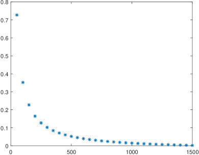
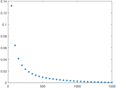
we plot the functions and . As it can be seen, the convergence to 0 is monotone and fast in both cases.
Test 2
In this test the two scenarios differ for the velocity functions rather than the initial conditions. We consider a road segment and the initial condition
We set , , , and we employ Dirichlet zero boundary conditions. Micro-simulations are run starting from the initial condition corresponding to the density function defined above. In Fig. 6
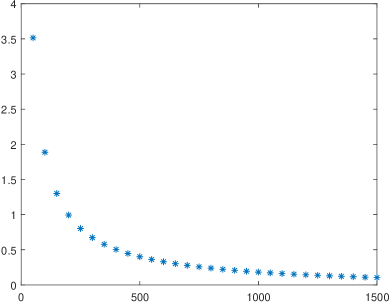
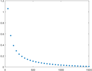
we plot the functions and . Again, the convergence to 0 is monotone and fast in both cases.
5 Comparing comparisons on a road network
5.1 Analytical results
The case of a road network is subtler and more difficult to categorize. The crucial difference is that, on some networks, vehicles loose their initial order (see Section 2.2.1), and, in parallel, the Wasserstein distance does not enjoy the property of monotone rearrangement. Therefore, analytical results described in the previous section are not expected to hold, at least for a general road network.
Example 5.1.
(soft counterexample). Let us consider the case of a merge, i.e. a simple network with one junction, two incoming roads and one outgoing road. Assume that vehicles are initially located on the two incoming roads only, as shown in Fig. 7, and that, at final time, all vehicles reach the outgoing road, merging one after the other, as shown in Fig. 9(top). Swapping the two initial conditions on the incoming roads, see Fig. 8, we get the solution shown in Fig. 9(bottom). It is clear that, in this case, we have since vehicles do not occupy the same positions in the two scenarios. At the same time, we have since, on the whole, vehicles do occupy the same positions.
Remark 5.2.
The case described above represents only a ’soft’ counterexample to Theorem 4.1. In fact, we still get the convergence for . This can be easily seen in Fig. 9, observing that, on a road with finite length filled with vehicles, the distance between one vehicle and the following one is . As a consequence, moving vehicles of mass for a distance costs in total
Example 5.3.
(hard counterexample). Let us consider again the case described in Example 5.1. Assume that in the first scenario vehicles are initially located as shown in Fig. 7, while, in the second scenario, vehicles on the first incoming road are moved to the left so much to be, at final time, all behind the last vehicle coming from the second incoming road, see Fig. 10.
In this case the difference between and is kept also in the limit for since the distance does not shrink to 0 in the limit (it must be larger than ).
5.2 Numerical results
In this section we aim at confirming the theoretical results presented above from the numerical point of view. As we did in Section 4.2, we run micro- and macro-simulations with different initial conditions and then we plot the function .
Test 3 (soft counterexample)
We consider the network of Example 5.1 where each road has length 20. On such a network, path 1 (resp., 2) joins the first (resp., second) incoming road with the outgoing road. The two slightly shifted initial conditions are
Note that vehicles are bumper-to-bumper. We also set , , and we employ Dirichlet zero boundary conditions. Micro-simulations are run starting from the initial conditions corresponding to the density functions defined above. In Fig. 11
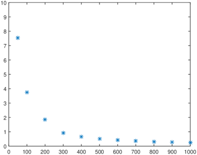
we plot the function at final time . As expected, the convergence is achieved also in this case.
Test 4 (hard counterexample)
We consider again the network of Example 5.1 where each road has length 30. The two shifted initial conditions are
We also set , , and we employ Dirichlet zero boundary conditions. Micro-simulations are run starting from the initial conditions corresponding to the density functions defined above. In Fig. 12
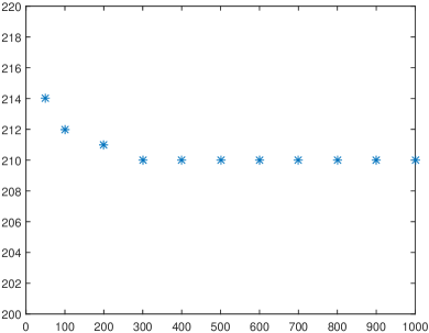
we plot the function at final time . As expected, the convergence is not achieved in this case.
6 Conclusions
In this paper we have investigated the problem of comparing traffic states in a multiscale framework. The notion of Wasserstein distance appears totally adequate in the case of single road simulations since it matches human intuition and it is totally independent of the scale of observation. In the case of a road network, instead, the microscopic Wasserstein distance is not the right notion of distance unless we stop distinguishing single vehicles, which is exactly what happens in the many-particle limit.
Acknowledgments
Authors want to thank Benedetto Piccoli for the useful discussions about the properties of the Wasserstein distance, and Andrea Tosin for the useful suggestions. Authors also thank the anonymous referees for their suggestions on the proof of Theorem 4.1.
E. Cristiani is a member of the INdAM Research group GNCS.
Author contributions
Both authors contributed equally to this work.
References
- 1 Aw A., Klar A., Rascle M., Materne T.. Derivation of continuum flow traffic models from microscopic follow-the-leader models. SIAM J. Appl. Math.. 2002;63:259-278.
- 2 Greenberg J. M.. Extensions and amplifications of a traffic model of Aw and Rascle. SIAM J. Appl. Math.. 2001;62:729-745.
- 3 Di Francesco M., Fagioli S., Rosini M. D.. Many particle approximation of the Aw-Rascle-Zhang second order model for vehicular traffic. Math. Biosci. Eng.. 2017;14(1):127-141.
- 4 Aw A., Rascle M.. Resurrection of “second order” models of traffic flow?. SIAM J. Appl. Math.. 2000;60:916-938.
- 5 Zhang H. M.. A non-equilibrium traffic model devoid of gas-like behavior. Transportation Res. Part B. 2002;36:275-290.
- 6 Helbing D.. Traffic and related self-driven many-particle systems. Rev. Mod. Phys.. 2001;73:1067-1141.
- 7 Pipes L. A.. An operational analysis of traffic dynamics. J. Appl. Phys.. 1953;24:274-281.
- 8 Colombo R. M., Rossi E.. On the micro-macro limit in traffic flow. Rend. Sem. Mat. Univ. Padova. 2014;131:217-235.
- 9 Rossi E.. A justification of a LWR model based on a follow the leader description. Discrete Contin. Dyn. Syst. Ser. S. 2014;7:579-591.
- 10 Di Francesco M., Rosini M. D.. Rigorous derivation of nonlinear scalar conservation laws from follow-the-leader type models via many particle limit. Arch. Rational Mech. Anal.. 2015;217:831-871.
- 11 Di Francesco M., Fagioli S., Rosini M. D.. Deterministic particle approximation of scalar conservation laws. Boll. Unione Mat. Ital.. 2017;10:487-501.
- 12 Lighthill M. J., Whitham G. B.. On kinematic waves II. A theory of traffic flow on long crowded roads. Proc. R. Soc. Lond. Ser. A. 1955;229:317-345.
- 13 Richards P. I.. Shock waves on the highway. Oper. Res.. 1956;4:42-51.
- 14 Forcadel N., Salazar W., Zaydan M.. Homogenization of second order discrete model with local perturbation and application to traffic. Discrete Contin. Dyn. Syst. Ser. A. 2017;37(3):1437-1487.
- 15 Forcadel N., Salazar W.. Homogenization of second order discrete model and application to traffic flow. Differential Integral Equations. 2015;28(11-12):1039-1068.
- 16 Cristiani E., Sahu S.. On the micro-to-macro limit for first-order traffic flow models on networks. Netw. Heterog. Media. 2016;11:395-413.
- 17 Hilliges M., Weidlich W.. A phenomenological model for dynamic traffic flow in networks. Transportation Res. Part B. 1995;29:407-431.
- 18 Briani M., Cristiani E.. An easy-to-use algorithm for simulating traffic flow on networks: Theoretical study. Netw. Heterog. Media. 2014;9:519-552.
- 19 Bretti G., Briani M., Cristiani E.. An easy-to-use algorithm for simulating traffic flow on networks: Numerical experiments. Discrete Contin. Dyn. Syst. Ser. S. 2014;7:379-394.
- 20 Cristiani E., Piccoli B., Tosin A.. Multiscale Modeling of Pedestrian Dynamics. Modeling, Simulation & ApplicationsSpringer; 2014.
- 21 Briani M., Cristiani E., Iacomini E.. Sensitivity analysis of the LWR model for traffic forecast on large networks using Wasserstein distance. Commun. Math. Sci.. 2018;16:123-144.
- 22 Bretti G., Natalini R., Piccoli B.. A fluid-dynamic traffic model on road networks. Arch. Comput. Methods Eng.. 2007;14:139-172.
- 23 Garavello M., Piccoli B.. Traffic Flow on Networks. AIMS Series on Applied Mathematics; 2006.
- 24 Coclite G. M., Garavello M., Piccoli B.. Traffic flow on a road network. SIAM J. Math. Anal.. 2005;36:1862-1886.
- 25 Garavello M., Piccoli B.. Source-destination flow on a road network. Comm. Math. Sci.. 2005;3:261-283.
- 26 Garavello M., Goatin P.. The Cauchy problem at a node with buffer. Discrete Contin. Dyn. Syst. Ser. A. 2012;32(6):1915-1938.
- 27 Garavello M., Piccoli B.. Advances in Dynamic Network Modeling in Complex Transportation Systems Complex Networks and Dynamic Systems, vol. 2: ch. A multibuffer model for LWR road networks, :143-161. Springer 2013.
- 28 Herty M., Lebacque J.-P., Moutari S.. A novel model for intersections of vehicular traffic flow. Netw. Heterog. Media. 2009;4:813-826.
- 29 Villani C.. Optimal Transport: Old and New Grundlehren der Mathematischen Wissenschaften [Fundamental Principles of Mathematical Sciences], vol. 338: . Berlin: Springer-Verlag; 2009.
- 30 Villani C.. Topics in Optimal Transportation Graduate Studies in Mathematics Series, vol. 58: . American Mathematical Society; 2003.
- 31 Santambrogio F.. Optimal Transport for Applied Mathematicians. Calculus of Variations, PDEs, and Modeling. Birkhäuser; 2015.
- 32 Sinha S. M.. Mathematical Programming: Theory and Methods. Elsevier Science & Technology Books; 2006.
- 33 Benamou J.-D., Brenier Y.. A computational fluid mechanics solution to the Monge-Kantorovich mass transfer problem. Numerische Mathematik. 2000;84(3):375-393.
- 34 Mazón J. M., Rossi J. D., Toledo J.. Optimal mass transport on metric graphs. SIAM J. Optim.. 2015;25:1609-1632.
- 35 Dijkstra E. W.. A note on two problems in connexion with graphs. Numerische Mathematik. 1959;1:269-271.
- 36 Dafermos C. M.. Hyperbolic conservation laws in continuum physics Grundlehren der mathematischen Wissenschaften, vol. 325: . Springer-Verlag Berlin Heidelberg; iv ed.2016.