Effective field theory for collective rotations and vibrations of triaxially deformed nuclei

Abstract

The effective field theory (EFT) for triaxially deformed even-even nuclei is generalized to include the vibrational degrees of freedom. The pertinent Hamiltonian is constructed up to next-to-leading order. The leading order part describes the vibrational motion, and the NLO part couples rotations to vibrations. The applicability of the EFT Hamiltonian is examined through the description of the energy spectra of the ground state bands, $\gamma$-bands, and $K=4$ bands in the ^108,110,112Ru isotopes. It is found that by taking into account the vibrational degrees of freedom, the deviations for high-spin states in the $\gamma$-band observed in the EFT with only rotational degrees of freedom disappear. This supports the importance of including vibrational degrees of freedom in the EFT formulation for the collective motion of triaxially deformed nuclei.

I Introduction

Effective field theory (EFT) is based on symmetry principles alone, and it exploits the separation of energy scales for the systematic construction of the Hamiltonian supplemented by a power counting. In this way, an increase in the number of parameters (i.e., low-energy constants that need to be adjusted to data) goes hand in hand with an increase in precision and thereby counter balances the partial loss of predictive power. Actually, EFT often exhibits an impressive efficiency as highlighted by analytical results and economical means of calculations. In recent decades, EFT has enjoyed considerable successes in low-energy hadronic and nuclear structure physics. Pertinent examples include the descriptions of the nuclear interactions Epelbaum (2006); Epelbaum et al. (2009); Machleidt and Entem (2011), halo nuclei Bertulani et al. (2002); Hammer and Phillips (2011); Ryberg et al. (2014), and nuclear few-body systems Bedaque and van Kolck (2002); Grießhammer et al. (2012); Hammer et al. (2013). Recently, Papenbrock and his collaborators have developed an EFT to describe the collective rotational and vibrational motions of deformed nuclei by Papenbrock (2011); Zhang and Papenbrock (2013); Papenbrock and Weidenmüller (2014, 2015, 2016); Coello Pérez and Papenbrock (2015a, b); Coello Pérez and Papenbrock (2016).

Collective rotations and vibrations are the typical low-lying excitation modes of a nucleus. For a spherical nucleus, only vibrational modes exist. On the other hand, for a deformed nucleus, various vibrational bands are observed, and rotational bands are found to be built on the successive vibrational modes Bohr and Mottelson (1975); Ring and Schuck (1980). Since the initial paper in 2011 Papenbrock (2011), Papenbrock and his collaborators have completed a series of works devoted to the systematic treatment of nuclear collective motion in the EFT framework Zhang and Papenbrock (2013); Papenbrock and Weidenmüller (2014, 2015, 2016); Coello Pérez and Papenbrock (2015a, b); Coello Pérez and Papenbrock (2016). Through the application of EFT to deformed nuclei, the finer details of the experimental energy spectra, such as the change of the moment of inertia with spin, can be addressed properly through higher-order correction terms Papenbrock (2011); Zhang and Papenbrock (2013); Papenbrock and Weidenmüller (2014, 2015, 2016). Moreover, in this approach the uncertainties of the theoretical model can be quantified Coello Pérez and Papenbrock (2015b), and a consistent treatment of electroweak currents together with the Hamiltonian can be obtained Coello Pérez and Papenbrock (2015a). Let us note that all these investigations were restricted to axially symmetric nuclei.

Very recently, the pertinent EFT has been further generalized to describe the rotational motion of triaxially deformed even-even nuclei Chen et al. (2017). The triaxial deformation of nucleus has been a subject of much interest in the theoretical study of nuclear structure for a long time. It is related to many interesting phenomena, including the $\gamma$-band Bohr and Mottelson (1975), signature inversion Bengtsson et al. (1984), anomalous signature splitting Hamamoto and Sagawa (1988), the wobbling motion Bohr and Mottelson (1975), chiral rotational modes Frauendorf and Meng (1997) and most prominently multiple chiral doublet bands Meng et al. (2006). In fact, the wobbling motion and chiral doublet bands are regarded as unique fingerprints of stable triaxially deformed nuclei. In Ref. Chen et al. (2017), the pertinent Hamiltonian has been constructed up to next-to-leading order (NLO). Taking the energy spectra of the ground state and $\gamma$- bands (together with some $K=4$ bands) in the ^102-112Ru isotopes as examples, the applicability of this novel EFT for triaxial nuclei has been examined. It has been found that the description at NLO is overall better than at leading order (LO). Nevertheless, there were still some deviations between the NLO calculation and the data for some high-spin states in the $\gamma$-bands. The comparison to the results of a five-dimensional collective Hamiltonian (5DCH) based on the covariant density functional theory (CDFT) Meng (2016) has indicated that the inclusion of vibrational degrees of freedom in the EFT formulation is important.

Therefore, in this paper, the vibrational degrees of freedom are additionally considered in the formulation of an EFT for collective nuclear motion. The pertinent Hamiltonian will be constructed up to NLO, where the LO part describes the vibrational motion, and the NLO part couples rotations to vibrations. The energy spectra of ground state bands, $\gamma$-bands, and $K=4$ bands in the ^108,110,112Ru isotopes are taken as examples to examine the applicability of our extended EFT approach.

The present paper is organized as follows. In Sec. II, the EFT for collective rotations and vibrations of triaxially deformed nuclei is constructed. The solutions of the rotational Hamiltonian in first order perturbation theory are given in Sec. III. The obtained vibrational Hamiltonian is reduced in Sec. IV by expressing it in terms of the quadrupole deformation parameters $\beta_{2}$ and $\gamma_{2}$. The results of the corresponding quantum-mechanical calculations are presented and discussed in detail in Sec. V. Finally, a summary is given in Sec. VI together with perspectives for future research directions.

II Construction of the EFT

In this section, the procedure of constructing the effective Lagrangian and Hamiltonian for collective rotations and vibrations is introduced and carried out. It follows similar steps as in the case of axially symmetric nuclei studied in Refs. Papenbrock and Weidenmüller (2014, 2015) and in the case of collective rotations of triaxially deformed nuclei investigated in Ref. Chen et al. (2017).

II.1 Dynamical variables

In an EFT, the symmetry is (typically) realized nonlinearly Coleman et al. (1969); Callan et al. (1969), and the Nambu-Goldstone fields parametrize the coset space $\mathcal{G}/\mathcal{H}$. Here, $\mathcal{G}$ is the symmetry group of the Hamiltonian and $\mathcal{H}$ the symmetry group of the ground state, is a proper subgroup of $\mathcal{G}$. The effective Lagrangian $\mathcal{L}$ is built from invariants that can be constructed from the fields in the coset space. In the following, we will write the fields relevant for collective nuclear motion in the space-fixed coordinate frame, where the three generators of infinitesimal rotations about the space-fixed $x$, $y$, and $z$-axes are denoted by $J_{x}$, $J_{y}$, and $J_{z}$.

To describe a global rotation, the three Euler angles $\alpha$, $\beta$, and $\gamma$ serve as natural dynamical variables. On the classical level, they are purely time-dependent and upon quantization, they give rise to rotational bands. On the other hand, vibrations act locally on the nuclear surface and its location can be described by body-fixed spherical coordinates $r$, $\theta$, and $\phi$. Following the arguments in Refs. Papenbrock and Weidenmüller (2014, 2015, 2016), one expects that Nambu-Goldstone modes related to the radial coordinate $r$ have higher frequencies than those related to the angles $\theta$ and $\phi$. For low energy excitations, one can therefore restrict the attention to the angular variables.

A triaxially deformed nucleus is invariant under the $180^{\circ}$ rotation about the body-fixed axes (discrete $\textrm{D}_{2}$ symmetry), while the continuous $\textrm{SO}(3)$ symmetry is broken by the deformation. Consequently, the Nambu-Goldstone modes lie in the three-dimensional coset space $\textrm{SO}(3)/\textrm{D}_{2}$. The modes depend on the angles $\theta$ and $\phi$ and the time $t$ and are generated from the nuclear ground state by a unitary transformation $U$. Following Refs. Papenbrock and Weidenmüller (2014, 2015, 2016); Chen et al. (2017), the matrix $U$ can be parameterized in a product form as

$$U =g(\alpha,\beta,\gamma)u(x,y,z),$$

$$g(\alpha,\beta,\gamma) =\exp\{-i\alpha(t)J_{z}\}\exp\{-i\beta(t)J_{y}\}\exp\{-i\gamma(t)J_{z}\},$$

$$u(x,y,z) =\exp\{-ix(\theta,\phi,t)J_{x}-iy(\theta,\phi,t)J_{y}-iz(\theta,\phi,t)J_{z}\}.$$ (1)

The fields $x(\theta,\phi,t)$, $y(\theta,\phi,t)$, and $z(\theta,\phi,t)$ with $|x|$, $|y|$, $|z|\ll 1$ generate small-amplitude vibrations of the nuclear surface. They depend on $\theta$ and $\phi$ in such that their angular averages vanish

$$\int d\Omega~{}x(\theta,\phi,t)=\int d\Omega~{}y(\theta,\phi,t)=\int d\Omega~{}z(\theta,\phi,t)=0,$$ (2)

where $d\Omega=\sin\theta\,d\theta d\phi$ denotes the surface element on the unit sphere. Note that in the axially symmetric case Papenbrock and Weidenmüller (2014, 2015), $\gamma(t)$ and $z(\theta,\phi,t)$ do not exist as observable degrees of freedom, since the operator $J_{z}$ acting on the axially deformed ground state gives zero.

The power counting underlying the EFT is specified by Papenbrock and Weidenmüller (2016)

$$\alpha,\beta,\gamma\sim\mathcal{O}(1),\quad\dot{\alpha},\dot{\beta},\dot{\gamma}\sim\xi,$$ (3)

$$x,y,z\sim\sqrt{\xi/\Omega},\quad\dot{x},\dot{y},\dot{z}\sim\sqrt{\xi\Omega},\quad\partial_{\nu}x,\partial_{\nu}y,\partial_{\nu}z\sim\sqrt{\xi/\Omega},$$ (4)

where the $\xi$ and the $\Omega$ denote the energy scales of the rotational and vibrational motion, respectively. The dot refers to a time derivative and $\partial_{\nu}$ to angular derivatives with $\nu=\theta$ or $\phi$. Note that $\xi$ (typically $\approx 80$ keV) is much smaller than $\Omega$ (typically $\approx$ 1 MeV), and hence $\sqrt{\xi/\Omega}\ll 1$ is a reasonably small parameter.

II.2 Effective Lagrangian

As usual, the effective Lagrangian is built from invariants. These are constructed from quantities $a_{\mu}^{x}$, $a_{\mu}^{y}$, and $a_{\mu}^{z}$ defined by Coleman et al. (1969); Callan et al. (1969); Papenbrock and Weidenmüller (2014, 2015); Chen et al. (2017)

$$iU^{-1}\partial_{\mu}U=a_{\mu}^{x}J_{x}+a_{\mu}^{y}J_{y}+a_{\mu}^{z}J_{z}.$$ (5)

The symbol $\partial_{\mu}$ stands for a derivative with respect to one of the variables $\theta$, $\phi$, and $t$.

To work out the Nambu-Goldstone modes explicitly, we use the decompositions

$$ig^{-1}\partial_{t}g =(-\dot{\alpha}\sin\beta\cos\gamma+\dot{\beta}\sin\gamma)J_{x}+(\dot{\alpha}\sin\beta\sin\gamma+\dot{\beta}\cos\gamma)J_{y}+(\dot{\alpha}\cos\beta+\dot{\gamma})J_{z},$$ (6)

and

$$iu^{-1}\partial_{t}u =\Big{\{}\dot{x}+\frac{1}{2}(\dot{y}z-y\dot{z})-\frac{1}{6}\Big{[}(y^{2}+z^{2})\dot{x}-x(y\dot{y}+z\dot{z})\Big{]}\Big{\}}J_{x}$$

$$\quad+\Big{\{}\dot{y}+\frac{1}{2}(\dot{z}x-z\dot{x})-\frac{1}{6}\Big{[}(x^{2}+z^{2})\dot{y}-y(x\dot{x}+z\dot{z})\Big{]}\Big{\}}J_{y}$$

$$\quad+\Big{\{}\dot{z}+\frac{1}{2}(\dot{x}y-x\dot{y})-\frac{1}{6}\Big{[}(x^{2}+y^{2})\dot{z}-z(x\dot{x}+y\dot{y})\Big{]}\Big{\}}J_{z}~{}.$$ (7)

In the calculation of $iu^{-1}\partial_{t}u$, the expansion of $u$ in powers of $x$, $y$, $z$ has been performed up to cubic terms. With these formula, one obtains for the time derivative

$$iU^{-1}\partial_{t}U =iu^{-1}\partial_{t}u+iu^{-1}(g^{-1}\partial_{t}g)u$$

$$=\Big{\{}\dot{x}+\frac{1}{2}(\dot{y}z-y\dot{z})-\frac{1}{6}\Big{[}(y^{2}+z^{2})\dot{x}-x(y\dot{y}+z\dot{z})\Big{]}+(-\dot{\alpha}\sin\beta\cos\gamma+\dot{\beta}\sin\gamma)$$

$$\quad+(\dot{\alpha}\sin\beta\sin\gamma+\dot{\beta}\cos\gamma)z-(\dot{\alpha}\cos\beta+\dot{\gamma})y\Big{\}}J_{x}$$

$$\quad+\Big{\{}\dot{y}+\frac{1}{2}(\dot{z}x-z\dot{x})-\frac{1}{6}\Big{[}(x^{2}+z^{2})\dot{y}-y(x\dot{x}+z\dot{z})\Big{]}+(\dot{\alpha}\sin\beta\sin\gamma+\dot{\beta}\cos\gamma)$$

$$\quad+(\dot{\alpha}\cos\beta+\dot{\gamma})x-(-\dot{\alpha}\sin\beta\cos\gamma+\dot{\beta}\sin\gamma)z\Big{\}}J_{y}$$

$$\quad+\Big{\{}\dot{z}+\frac{1}{2}(\dot{x}y-x\dot{y})-\frac{1}{6}\Big{[}(x^{2}+y^{2})\dot{z}-z(x\dot{x}+y\dot{y})\Big{]}+(\dot{\alpha}\cos\beta+\dot{\gamma})$$

$$\quad+(-\dot{\alpha}\sin\beta\cos\gamma+\dot{\beta}\sin\gamma)y-(\dot{\alpha}\sin\beta\sin\gamma+\dot{\beta}\cos\gamma)x\Big{\}}J_{z},$$ (8)

while the angular derivatives ($\nu=\theta,\phi$) read

$$iU^{-1}\partial_{\nu}U =iu^{-1}\partial_{\nu}u$$

$$=\Big{\{}\partial_{\nu}x+\frac{1}{2}(z\partial_{\nu}y-y\partial_{\nu}z)-\frac{1}{6}\Big{[}(y^{2}+z^{2})\partial_{\nu}x-x(y\partial_{\nu}y+z\partial_{\nu}z)\Big{]}\Big{\}}J_{x}$$

$$\quad+\Big{\{}\partial_{\nu}y+\frac{1}{2}(x\partial_{\nu}z-z\partial_{\nu}x)-\frac{1}{6}\Big{[}(x^{2}+z^{2})\partial_{\nu}y-y(x\partial_{\nu}x+z\partial_{\nu}z)\Big{]}\Big{\}}J_{y}$$

$$\quad+\Big{\{}\partial_{\nu}z+\frac{1}{2}(y\partial_{\nu}x-x\partial_{\nu}y)-\frac{1}{6}\Big{[}(x^{2}+y^{2})\partial_{\nu}z-z(x\partial_{\nu}x+y\partial_{\nu}y)\Big{]}\Big{\}}J_{z}.$$ (9)

In the expansions of $iU^{-1}\partial_{t}U$ in Eq. (II.2) we go up to order $\xi\sqrt{\xi/\Omega}$ to include the coupling terms between rotations and vibrations. Therefore, the quantities $u^{-1}J_{x}u$, $u^{-1}J_{y}u$, and $u^{-1}J_{z}u$ need to be expanded only up to order $\sqrt{\xi/\Omega}$, since $g^{-1}\partial_{t}g$ is of order $\xi$.

The components of the angular velocities follow from Eqs. (5) and (II.2) as

$$a_{t}^{x} =\dot{x}+\Big{[}\frac{1}{2}(\dot{y}z-y\dot{z})+(-\dot{\alpha}\sin\beta\cos\gamma+\dot{\beta}\sin\gamma)\Big{]}+\Big{\{}-\frac{1}{6}\Big{[}(y^{2}+z^{2})\dot{x}-x(y\dot{y}+z\dot{z})\Big{]}$$

$$\quad+(\dot{\alpha}\sin\beta\sin\gamma+\dot{\beta}\cos\gamma)z-(\dot{\alpha}\cos\beta+\dot{\gamma})y\Big{\}},$$ (10)

$$a_{t}^{y} =\dot{y}+\Big{[}\frac{1}{2}(\dot{z}x-z\dot{x})+(\dot{\alpha}\sin\beta\sin\gamma+\dot{\beta}\cos\gamma)\Big{]}+\Big{\{}-\frac{1}{6}\Big{[}(x^{2}+z^{2})\dot{y}-y(x\dot{x}+z\dot{z})\Big{]}$$

$$\quad+(\dot{\alpha}\cos\beta+\dot{\gamma})x-(-\dot{\alpha}\sin\beta\cos\gamma+\dot{\beta}\sin\gamma)z\Big{\}},$$ (11)

$$a_{t}^{z} =\dot{z}+\Big{[}\frac{1}{2}(\dot{x}y-x\dot{y})+(\dot{\alpha}\cos\beta+\dot{\gamma})\Big{]}+\Big{\{}-\frac{1}{6}\Big{[}(x^{2}+y^{2})\dot{z}-z(x\dot{x}+y\dot{y})\Big{]}$$

$$\quad+(-\dot{\alpha}\sin\beta\cos\gamma+\dot{\beta}\sin\gamma)y-(\dot{\alpha}\sin\beta\sin\gamma+\dot{\beta}\cos\gamma)x\Big{\}}~{},$$ (12)

where the leading terms ($\dot{x}$, $\dot{y}$, and $\dot{z}$) are of order $\sqrt{\xi\Omega}$. The terms in square brackets are proportional to the energy scale $\xi$, and those in curly brackets scale as $\xi\sqrt{\xi/\Omega}$. Thus, successive terms in $a_{t}^{x,y,z}$ are suppressed by a relative factor $\sqrt{\xi/\Omega}$.

Moreover, one obtains from Eqs. (5) and (II.2) for the components involving angular derivatives

$$a_{\nu}^{x} =\partial_{\nu}x+\frac{1}{2}(z\partial_{\nu}y-y\partial_{\nu}z)-\frac{1}{6}\Big{[}(y^{2}+z^{2})\partial_{\nu}x-x(y\partial_{\nu}y+z\partial_{\nu}z)\Big{]},$$ (13)

$$a_{\nu}^{y} =\partial_{\nu}y+\frac{1}{2}(x\partial_{\nu}z-z\partial_{\nu}x)-\frac{1}{6}\Big{[}(x^{2}+z^{2})\partial_{\nu}y-y(x\partial_{\nu}x+z\partial_{\nu}z)\Big{]},$$ (14)

$$a_{\nu}^{z} =\partial_{\nu}z+\frac{1}{2}(y\partial_{\nu}x-x\partial_{\nu}y)-\frac{1}{6}\Big{[}(x^{2}+y^{2})\partial_{\nu}z-z(x\partial_{\nu}x+y\partial_{\nu}y)\Big{]},$$ (15)

where the leading terms ($\partial_{\nu}x$, $\partial_{\nu}y$, and $\partial_{\nu}z$) scale as $\sqrt{\xi/\Omega}$, the terms in round brackets as $\xi/\Omega$, and those square brackets as $(\xi/\Omega)^{3/2}$. Again, successive terms in $a_{\nu}^{x,y,z}$ are suppressed by a relative factor $\sqrt{\xi/\Omega}$.

The expressions in Eqs. (II.2)-(15) give the lowest order contributions from the Nambu-Goldstone modes $x,y,z$ and $\alpha,\beta,\gamma$ introduced in Eq. (II.1). Note that if $\gamma=0$ and $z=0$, then one recovers the axailly symmetric case Papenbrock and Weidenmüller (2014, 2015).

Respecting time-reversal invariance and the discrete $D_{2}$ symmetry of a triaxial nucleus , only the squares of $a_{\mu}^{x}$, $a_{\mu}^{y}$, and $a_{\mu}^{z}$ may be used to construct the Lagrangian. For the temporal parts, one gets

$$(a_{t}^{x})^{2} =(-\dot{\alpha}\sin\beta\cos\gamma+\dot{\beta}\sin\gamma)^{2}$$

$$\quad+\dot{x}^{2}+(\dot{y}z-y\dot{z})(-\dot{\alpha}\sin\beta\cos\gamma+\dot{\beta}\sin\gamma)$$

$$\quad+2(\dot{\alpha}\sin\beta\sin\gamma+\dot{\beta}\cos\gamma)\dot{x}z-2(\dot{\alpha}\cos\beta+\dot{\gamma})\dot{x}y$$

$$\quad+\frac{1}{4}(\dot{y}z-y\dot{z})^{2}-\frac{1}{3}\Big{[}(y^{2}+z^{2})\dot{x}^{2}-x\dot{x}(y\dot{y}+z\dot{z})\Big{]},$$ (16)

$$(a_{t}^{y})^{2} =(\dot{\alpha}\sin\beta\sin\gamma+\dot{\beta}\cos\gamma)^{2}$$

$$\quad+\dot{y}^{2}+(\dot{z}x-z\dot{x})(\dot{\alpha}\sin\beta\sin\gamma+\dot{\beta}\cos\gamma)$$

$$\quad+2(\dot{\alpha}\cos\beta+\dot{\gamma})\dot{y}x-2(-\dot{\alpha}\sin\beta\cos\gamma+\dot{\beta}\sin\gamma)\dot{y}z$$

$$\quad+\frac{1}{4}(\dot{z}x-z\dot{x})^{2}-\frac{1}{3}\Big{[}(x^{2}+z^{2})\dot{y}^{2}-y\dot{y}(x\dot{x}+z\dot{z})\Big{]},$$ (17)

$$(a_{t}^{z})^{2} =(\dot{\alpha}\cos\beta+\dot{\gamma})^{2}$$

$$\quad+\dot{z}^{2}+(\dot{x}y-x\dot{y})(\dot{\alpha}\cos\beta+\dot{\gamma})$$

$$\quad+2(-\dot{\alpha}\sin\beta\cos\gamma+\dot{\beta}\sin\gamma)\dot{z}y-2(\dot{\alpha}\sin\beta\sin\gamma+\dot{\beta}\cos\gamma)\dot{z}x$$

$$\quad+\frac{1}{4}(\dot{x}y-x\dot{y})^{2}-\frac{1}{3}\Big{[}(x^{2}+y^{2})\dot{z}^{2}-z\dot{z}(x\dot{x}+y\dot{y})\Big{]},$$ (18)

where terms of order $\xi\Omega(\xi/\Omega)^{3/2}$ and higher have been consistently dropped. The invariants in Eqs. (II.2)-(II.2) can still be decomposed according to the power of the vibrational fields into

$$\mathcal{L}_{1a} =(-\dot{\alpha}\sin\beta\cos\gamma+\dot{\beta}\sin\gamma)^{2},$$ (19)

$$\mathcal{L}_{2a} =\dot{x}^{2}+(\dot{y}z-y\dot{z})(-\dot{\alpha}\sin\beta\cos\gamma+\dot{\beta}\sin\gamma)$$

$$\quad+2(\dot{\alpha}\sin\beta\sin\gamma+\dot{\beta}\cos\gamma)\dot{x}z-2(\dot{\alpha}\cos\beta+\dot{\gamma})\dot{x}y,$$ (20)

$$\mathcal{L}_{3a} =\frac{1}{4}(\dot{y}z-y\dot{z})^{2}-\frac{1}{3}\Big{[}(y^{2}+z^{2})\dot{x}^{2}-x\dot{x}(y\dot{y}+z\dot{z})\Big{]},$$ (21)

$$\mathcal{L}_{1b} =(\dot{\alpha}\sin\beta\sin\gamma+\dot{\beta}\cos\gamma)^{2},$$ (22)

$$\mathcal{L}_{2b} =\dot{y}^{2}+(\dot{z}x-z\dot{x})(\dot{\alpha}\sin\beta\sin\gamma+\dot{\beta}\cos\gamma)$$

$$\quad+2(\dot{\alpha}\cos\beta+\dot{\gamma})\dot{y}x-2(-\dot{\alpha}\sin\beta\cos\gamma+\dot{\beta}\sin\gamma)\dot{y}z,$$ (23)

$$\mathcal{L}_{3b} =\frac{1}{4}(\dot{z}x-z\dot{x})^{2}-\frac{1}{3}\Big{[}(x^{2}+z^{2})\dot{y}^{2}-y\dot{y}(x\dot{x}+z\dot{z})\Big{]},$$ (24)

$$\mathcal{L}_{1c} =(\dot{\alpha}\cos\beta+\dot{\gamma})^{2},$$ (25)

$$\mathcal{L}_{2c} =\dot{z}^{2}+(\dot{x}y-x\dot{y})(\dot{\alpha}\cos\beta+\dot{\gamma})$$

$$\quad+2(-\dot{\alpha}\sin\beta\cos\gamma+\dot{\beta}\sin\gamma)\dot{z}y-2(\dot{\alpha}\sin\beta\sin\gamma+\dot{\beta}\cos\gamma)\dot{z}x,$$ (26)

$$\mathcal{L}_{3c} =\frac{1}{4}(\dot{x}y-x\dot{y})^{2}-\frac{1}{3}\Big{[}(x^{2}+y^{2})\dot{z}^{2}-z\dot{z}(x\dot{x}+y\dot{y})\Big{]},$$ (27)

where $\mathcal{L}_{1a,3a}$, $\mathcal{L}_{1b,3b}$, and $\mathcal{L}_{1c,3c}$ are of order $\xi^{2}$. The leading terms ($\dot{x}^{2}$, $\dot{y}^{2}$, and $\dot{z}^{2}$) in $\mathcal{L}_{2a,2b,2c}$ are of order $\xi\Omega$ and the remaining terms scale as order $\xi^{2}$.

Next, we turn to the invariants constructed from derivatives with respect to the angles $\theta$ and $\phi$ listed in Eqs. (13)-(15). We restrict ourselves to terms of up to fourth order in $x$, $y$, $z$, and their derivatives. The pertinent squares read

$$(a_{\nu}^{x})^{2} =(\partial_{\nu}x)^{2}+\Big{[}(\partial_{\nu}x)(z\partial_{\nu}y-y\partial_{\nu}z)\Big{]}$$

$$\quad+\Big{\{}\frac{1}{4}(z\partial_{\nu}y-y\partial_{\nu}z)^{2}-\frac{1}{3}(\partial_{\nu}x)\Big{[}(y^{2}+z^{2})\partial_{\nu}x-x(y\partial_{\nu}y+z\partial_{\nu}z)\Big{]}\Big{\}},$$ (28)

$$(a_{\nu}^{y})^{2} =(\partial_{\nu}y)^{2}+\Big{[}(\partial_{\nu}y)(x\partial_{\nu}z-z\partial_{\nu}x)\Big{]}$$

$$\quad+\Big{\{}\frac{1}{4}(x\partial_{\nu}z-z\partial_{\nu}x)^{2}-\frac{1}{3}(\partial_{\nu}y)\Big{[}(x^{2}+z^{2})\partial_{\nu}y-y(x\partial_{\nu}x+z\partial_{\nu}z)\Big{]}\Big{\}},$$ (29)

$$(a_{\nu}^{z})^{2} =(\partial_{\nu}z)^{2}+\Big{[}(\partial_{\nu}z)(y\partial_{\nu}x-x\partial_{\nu}y)\Big{]}$$

$$\quad+\Big{\{}\frac{1}{4}(y\partial_{\nu}x-x\partial_{\nu}y)^{2}-\frac{1}{3}(\partial_{\nu}z)\Big{[}(x^{2}+y^{2})\partial_{\nu}z-z(x\partial_{\nu}x+y\partial_{\nu}y)\Big{]}\Big{\}},$$ (30)

where terms of order $(\xi/\Omega)^{5/2}$ and higher have been consistently dropped. In the above, $(a_{\nu}^{x})^{2}$, $(a_{\nu}^{y})^{2}$, and $(a_{\nu}^{z})^{2}$ are expressed in terms of $x$, $y$, $z$, and their derivatives as polynomials of degree two, three, and four, respectively.

The partial derivatives $\partial_{\nu}$ can be replaced by the orbital angular momenta operators $\bm{L}$, whose components are

$$L_{x} =i(\sin\phi~{}\partial_{\theta}+\cot\theta\cos\phi~{}\partial_{\phi}),$$ (31)

$$L_{y} =i(-\cos\phi~{}\partial_{\theta}+\cot\theta\sin\phi~{}\partial_{\phi}),$$ (32)

$$L_{z} =-i\partial_{\phi}.$$ (33)

By reexpressing $\partial_{\theta}$ and $\partial_{\phi}$ in terms of $L_{x}$, $L_{y}$, and $L_{z}$, one constructs from the first terms in Eqs. (II.2)-(II.2) the following six Lagrangians

$$\mathcal{L}_{4a} =(\bm{L}x)^{2},\quad\mathcal{L}_{4b}=(\bm{L}y)^{2},\quad\mathcal{L}_{4c}=(\bm{L}z)^{2},$$ (34)

$$\mathcal{L}_{4d} =(L_{z}x)^{2},\quad\mathcal{L}_{4e}=(L_{z}y)^{2},\quad\mathcal{L}_{4f}=(L_{z}z)^{2}.$$ (35)

In the same way, the second terms in square brackets lead to

$$\mathcal{L}_{5a} =(\bm{L}x)\big{[}z(\bm{L}y)-y(\bm{L}z)\big{]},$$ (36)

$$\mathcal{L}_{5b} =(\bm{L}y)\big{[}x(\bm{L}z)-z(\bm{L}x)\big{]},$$ (37)

$$\mathcal{L}_{5c} =(\bm{L}z)\big{[}y(\bm{L}x)-x(\bm{L}y)\big{]},$$ (38)

$$\mathcal{L}_{5d} =(L_{y}x)\big{[}z(L_{x}y)-y(L_{x}z)\big{]}+(L_{x}x)\big{[}z(L_{y}y)-y(L_{y}z)\big{]},$$ (39)

$$\mathcal{L}_{5e} =(L_{y}y)\big{[}x(L_{x}z)-z(L_{x}x)\big{]}+(L_{x}y)\big{[}x(L_{y}z)-z(L_{y}x)\big{]},$$ (40)

$$\mathcal{L}_{5f} =(L_{y}z)\big{[}y(L_{x}x)-x(L_{x}y)\big{]}+(L_{x}z)\big{[}y(L_{y}x)-x(L_{y}y)\big{]},$$ (41)

and the third terms in curly brackets give rise to

$$\mathcal{L}_{6a} =\frac{1}{4}\big{[}z(\bm{L}y)-y(\bm{L}z)\big{]}^{2}+\frac{1}{3}(\bm{L}x)\big{\{}x\big{[}y(\bm{L}y)+z(\bm{L}z)\big{]}-(y^{2}+z^{2})(\bm{L}x)\big{\}},$$ (42)

$$\mathcal{L}_{6b} =\frac{1}{4}\big{[}x(\bm{L}z)-z(\bm{L}x)\big{]}^{2}+\frac{1}{3}(\bm{L}y)\big{\{}y\big{[}z(\bm{L}z)+x(\bm{L}x)\big{]}-(z^{2}+x^{2})(\bm{L}y)\big{\}},$$ (43)

$$\mathcal{L}_{6c} =\frac{1}{4}\big{[}y(\bm{L}x)-x(\bm{L}y)\big{]}^{2}+\frac{1}{3}(\bm{L}z)\big{\{}z\big{[}x(\bm{L}x)+y(\bm{L}y)\big{]}-(x^{2}+y^{2})(\bm{L}z)\big{\}},$$ (44)

$$\mathcal{L}_{6d} =\frac{1}{2}\big{[}z(L_{y}y)-y(L_{y}z)\big{]}\big{[}z(L_{x}y)-y(L_{x}z)\big{]}+\frac{1}{3}x\big{\{}(L_{y}x)\big{[}y(L_{x}y)+z(L_{x}z)\big{]}$$

$$\quad+(L_{x}x)\big{[}y(L_{y}y)+z(L_{y}z)\big{]}\big{\}}-\frac{2}{3}(y^{2}+z^{2})(L_{x}x)(L_{y}x),$$ (45)

$$\mathcal{L}_{6e} =\frac{1}{2}\big{[}x(L_{y}z)-z(L_{y}x)\big{]}\big{[}x(L_{x}z)-z(L_{x}x)\big{]}+\frac{1}{3}y\big{\{}(L_{y}y)\big{[}z(L_{x}z)+x(L_{x}x)\big{]}$$

$$\quad+(L_{x}y)\big{[}z(L_{y}z)+x(L_{y}x)\big{]}\big{\}}-\frac{2}{3}(z^{2}+x^{2})(L_{x}y)(L_{y}y),$$ (46)

$$\mathcal{L}_{6f} =\frac{1}{2}\big{[}y(L_{y}x)-x(L_{y}y)\big{]}\big{[}y(L_{x}x)-x(L_{x}y)\big{]}+\frac{1}{3}z\big{\{}(L_{y}z)\big{[}x(L_{x}x)+y(L_{x}y)\big{]}$$

$$\quad+(L_{x}z)\big{[}x(L_{y}x)+y(L_{y}y)\big{]}\big{\}}-\frac{2}{3}(x^{2}+y^{2})(L_{x}z)(L_{y}z).$$ (47)

As a result, the total effective Lagrangian $L$ is given by the angular average of a arbitrary linear combination of the invariants constructed above and it involves 27 low-energy constants (LECs)

$$L =L_{1}+L_{2}+L_{3}+L_{4}+L_{5}+L_{6}$$

$$=\frac{1}{4\pi}\int d\Omega\Big{[}\sum_{i=a,b,c}\Big{(}\frac{A_{i}}{2}\mathcal{L}_{1i}+\frac{B_{i}}{2}\mathcal{L}_{2i}+\frac{C_{i}}{2}\mathcal{L}_{3i}\Big{)}-\sum_{i=a,b,c,d,e,f}\Big{(}\frac{D_{i}}{2}\mathcal{L}_{4i}+\frac{E_{i}}{2}\mathcal{L}_{5i}+\frac{F_{i}}{2}\mathcal{L}_{6i}\Big{)}\Big{]}.$$ (48)

Following Ref. Papenbrock and Weidenmüller (2014), we expand the real function $x(\theta,\phi,t)$ in terms of the real orthonormal functions $Z_{\lambda\mu}$, called tesseral harmonics, as

$$x(\theta,\phi,t)=\sum_{\lambda=2}^{\infty}\sum_{\mu=-\lambda}^{\lambda}x_{\lambda\mu}(\theta,\phi,t)Z_{\lambda\mu}(\theta,\phi),$$ (49)

and in the same way for the real variables $y$, $z$, $\dot{x}$, $\dot{y}$, and $\dot{z}$. The tesseral harmonics $Z_{\lambda\mu}(\theta,\phi)$ are related to the spherical harmonics $Y_{\lambda\mu}(\theta,\phi)$ by

$$Z_{\lambda\mu}=\left\{\begin{array}[]{ll}\displaystyle\frac{1}{\sqrt{2}}\Big{(}Y_{\lambda\mu}+Y_{\lambda\mu}^{*}\Big{)},&\mu>0,\\ Y_{\lambda 0},&\mu=0,\\ \displaystyle-\frac{i}{\sqrt{2}}\Big{(}Y_{\lambda\mu}-Y_{\lambda\mu}^{*}\Big{)},&\mu<0.\\ \end{array}\right.$$ (53)

It is obvious that the expansion coefficients $x_{\lambda\mu}$ are real. Note that in Eq. (49) the contributions with $\lambda=0$ and $\lambda=1$ must be excluded, since $\lambda=0$ describes global rotations while $\lambda=1$ describes global translations in space.

Using these expansions and carrying out the solid angle integration, the total Lagrangian takes the form

$$L =\frac{A_{a}}{2}\omega_{x}^{2}+\frac{A_{b}}{2}\omega_{y}^{2}+\frac{A_{c}}{2}\omega_{z}^{2}$$

$$\quad+\frac{B_{a}}{2}\sum_{\lambda\mu}\Big{[}\dot{x}_{\lambda\mu}^{2}+(\dot{y}_{\lambda\mu}z_{\lambda\mu}-y_{\lambda\mu}\dot{z}_{\lambda\mu})\omega_{x}+2\omega_{y}\dot{x}_{\lambda\mu}z_{\lambda\mu}-2\omega_{z}\dot{x}_{\lambda\mu}y_{\lambda\mu}\Big{]}$$

$$\quad+\frac{B_{b}}{2}\sum_{\lambda\mu}\Big{[}\dot{y}_{\lambda\mu}^{2}+(\dot{z}_{\lambda\mu}x_{\lambda\mu}-z_{\lambda\mu}\dot{x}_{\lambda\mu})\omega_{y}+2\omega_{z}\dot{y}_{\lambda\mu}x_{\lambda\mu}-2\omega_{x}\dot{y}_{\lambda\mu}z_{\lambda\mu}\Big{]}$$

$$\quad+\frac{B_{c}}{2}\sum_{\lambda\mu}\Big{[}\dot{z}_{\lambda\mu}^{2}+(\dot{x}_{\lambda\mu}y_{\lambda\mu}-x_{\lambda\mu}\dot{y}_{\lambda\mu})\omega_{z}+2\omega_{x}\dot{z}_{\lambda\mu}y_{\lambda\mu}-2\omega_{y}\dot{z}_{\lambda\mu}x_{\lambda\mu}\Big{]}$$

$$\quad-\frac{1}{2}\sum_{\lambda\mu}\Big{\{}\lambda(\lambda+1)\Big{[}D_{a}x_{\lambda\mu}^{2}+D_{b}y_{\lambda\mu}^{2}+D_{c}z_{\lambda\mu}^{2}\Big{]}+\mu^{2}\Big{[}D_{d}x_{\lambda\mu}^{2}+D_{e}y_{\lambda\mu}^{2}+D_{f}z_{\lambda\mu}^{2}\Big{]}\Big{\}}.$$ (54)

where we have restricted ourselves to terms up to orders with $\xi$, $\Omega$, and $\sqrt{\xi\Omega}$. In this way the number of LECs get reduced to 12. The pure rotor part (first line in Eq. (II.2)) is written in terms of squares of

$$\omega_{x} =-\dot{\alpha}\sin\beta\cos\gamma+\dot{\beta}\sin\gamma,$$ (55)

$$\omega_{y} =\dot{\alpha}\sin\beta\sin\gamma+\dot{\beta}\cos\gamma,$$ (56)

$$\omega_{z} =\dot{\alpha}\cos\beta+\dot{\gamma},$$ (57)

which are the rotational frequencies (in the body-fixed frame) expressed through Euler angles and their time derivatives Chen et al. (2017).

Finally, we study the dependence of the parameters on the energy scales. Since $\omega_{x,y,z}\sim\xi$, one requires $A_{a,b,c}\sim\xi^{-1}$ so that the rotational energy scales as order $\xi$. Similarly, $\dot{x}_{\lambda\mu}$, $\dot{y}_{\lambda\mu}$, $\dot{z}_{\lambda\mu}\sim\sqrt{\xi\Omega}$ leads to $B_{a,b,c}\sim\xi^{-1}$ so that the vibrational energy scales as order $\Omega$. This implies that the rotation-vibration coupling term is of order $\xi^{-1}\sqrt{\xi\Omega}\sqrt{\xi/\Omega}\xi=\xi$. In addition, the scaling behavior $D_{a-f}\sim\Omega^{2}/\xi$ implies that the collective potential (last line in Eq. (II.2)) is of order $\Omega$.

II.3 Canonical momenta

From the Lagrangian (II.2), one derives the following canonical momenta

$$p_{\alpha} =\frac{\partial L}{\partial\dot{\alpha}}=-\sin\beta\cos\gamma\Big{[}A_{a}\omega_{x}+\frac{B_{a}}{2}\sum_{\lambda\mu}(\dot{y}_{\lambda\mu}z_{\lambda\mu}-y_{\lambda\mu}\dot{z}_{\lambda\mu})-B_{b}\sum_{\lambda\mu}\dot{y}_{\lambda\mu}z_{\lambda\mu}+B_{c}\sum_{\lambda\mu}\dot{z}_{\lambda\mu}y_{\lambda\mu}\Big{]}$$

$$\quad+\sin\beta\sin\gamma\Big{[}A_{b}\omega_{y}+B_{a}\sum_{\lambda\mu}\dot{x}_{\lambda\mu}z_{\lambda\mu}+\frac{B_{b}}{2}\sum_{\lambda\mu}(\dot{z}_{\lambda\mu}x_{\lambda\mu}-z_{\lambda\mu}\dot{x}_{\lambda\mu})-B_{c}\sum_{\lambda\mu}\dot{z}_{\lambda\mu}x_{\lambda\mu}\Big{]}$$

$$\quad+\cos\beta\Big{[}A_{c}\omega_{z}-B_{a}\sum_{\lambda\mu}\dot{x}_{\lambda\mu}y_{\lambda\mu}+B_{b}\sum_{\lambda\mu}\dot{y}_{\lambda\mu}x_{\lambda\mu}+\frac{B_{c}}{2}\sum_{\lambda\mu}(\dot{x}_{\lambda\mu}y_{\lambda\mu}-x_{\lambda\mu}\dot{y}_{\lambda\mu})\Big{]},$$ (58)

$$p_{\beta} =\frac{\partial L}{\partial\dot{\beta}}=\sin\gamma\Big{[}A_{a}\omega_{x}+\frac{B_{a}}{2}\sum_{\lambda\mu}(\dot{y}_{\lambda\mu}z_{\lambda\mu}-y_{\lambda\mu}\dot{z}_{\lambda\mu})-B_{b}\sum_{\lambda\mu}\dot{y}_{\lambda\mu}z_{\lambda\mu}+B_{c}\sum_{\lambda\mu}\dot{z}_{\lambda\mu}y_{\lambda\mu}\Big{]}$$

$$\quad+\cos\gamma\Big{[}A_{b}\omega_{y}+B_{a}\sum_{\lambda\mu}\dot{x}_{\lambda\mu}z_{\lambda\mu}+\frac{B_{b}}{2}\sum_{\lambda\mu}(\dot{z}_{\lambda\mu}x_{\lambda\mu}-z_{\lambda\mu}\dot{x}_{\lambda\mu})-B_{c}\sum_{\lambda\mu}\dot{z}_{\lambda\mu}x_{\lambda\mu}\Big{]},$$ (59)

$$p_{\gamma} =\frac{\partial L}{\partial\dot{\gamma}}=A_{c}\omega_{z}-B_{a}\sum_{\lambda\mu}\dot{x}_{\lambda\mu}y_{\lambda\mu}+B_{b}\sum_{\lambda\mu}\dot{y}_{\lambda\mu}x_{\lambda\mu}+\frac{B_{c}}{2}\sum_{\lambda\mu}(\dot{x}_{\lambda\mu}y_{\lambda\mu}-x_{\lambda\mu}\dot{y}_{\lambda\mu}),$$ (60)

$$p_{\lambda\mu}^{x} =\frac{\partial L}{\partial\dot{x}_{\lambda\mu}}=B_{a}\Big{[}\dot{x}_{\lambda\mu}+\omega_{y}z_{\lambda\mu}-\omega_{z}y_{\lambda\mu}\Big{]}-\frac{B_{b}}{2}z_{\lambda\mu}\omega_{y}+\frac{B_{c}}{2}y_{\lambda\mu}\omega_{z},$$ (61)

$$p_{\lambda\mu}^{y} =\frac{\partial L}{\partial\dot{y}_{\lambda\mu}}=\frac{B_{a}}{2}z_{\lambda\mu}\omega_{x}+B_{b}\Big{[}\dot{y}_{\lambda\mu}+\omega_{z}x_{\lambda\mu}-\omega_{x}z_{\lambda\mu}\Big{]}-\frac{B_{c}}{2}x_{\lambda\mu}\omega_{z},$$ (62)

$$p_{\lambda\mu}^{z} =\frac{\partial L}{\partial\dot{z}_{\lambda\mu}}=-\frac{B_{a}}{2}y_{\lambda\mu}\omega_{x}+\frac{B_{b}}{2}x_{\lambda\mu}\omega_{y}+B_{c}\Big{[}\dot{z}_{\lambda\mu}+\omega_{x}y_{\lambda\mu}-\omega_{y}x_{\lambda\mu}\Big{]}.$$ (63)

Given the expressions of the canonical momenta $p_{\alpha}$, $p_{\beta}$, and $p_{\gamma}$, one obtains (by forming appropriate linear combinations) the components of angular momentum along the principal axes in the body-fixed frame

$$I_{1} =A_{a}\omega_{x}+\frac{B_{a}-2B_{b}}{2}\sum_{\lambda\mu}\dot{y}_{\lambda\mu}z_{\lambda\mu}+\frac{2B_{c}-B_{a}}{2}\sum_{\lambda\mu}y_{\lambda\mu}\dot{z}_{\lambda\mu},$$ (64)

$$I_{2} =A_{b}\omega_{y}+\frac{B_{b}-2B_{c}}{2}\sum_{\lambda\mu}\dot{z}_{\lambda\mu}x_{\lambda\mu}+\frac{2B_{a}-B_{b}}{2}\sum_{\lambda\mu}z_{\lambda\mu}\dot{x}_{\lambda\mu},$$ (65)

$$I_{3} =A_{c}\omega_{z}+\frac{B_{c}-2B_{a}}{2}\sum_{\lambda\mu}\dot{x}_{\lambda\mu}y_{\lambda\mu}+\frac{2B_{b}-B_{c}}{2}\sum_{\lambda\mu}x_{\lambda\mu}\dot{y}_{\lambda\mu}.$$ (66)

One observes that both rotation and vibration contribute to the angular momentum. For the rotation, these are the usual products of moment of inertia and rotational frequency $\omega_{x}$, $\omega_{y}$, or $\omega_{z}$. For the vibration, the additional angular momentum arises from the motion of the nuclear surface with (anisotropic) mass parameters $B_{a,b,c}$.

In the expressions for $p_{\lambda\mu}^{x}$, $p_{\lambda\mu}^{y}$, and $p_{\lambda\mu}^{z}$, terms such as $\dot{x}_{\lambda\mu}$ are of order $\sqrt{\xi\Omega}$, while cross terms such as $\omega_{y}z_{\lambda\mu}$ are of order $\xi\sqrt{\xi/\Omega}$. Since the latter ones are suppressed by a factor $\xi/\Omega$, we can safely drop them. This leads to

$$p_{\lambda\mu}^{x}=B_{a}\dot{x}_{\lambda\mu},\quad p_{\lambda\mu}^{y}=B_{b}\dot{y}_{\lambda\mu},\quad p_{\lambda\mu}^{z}=B_{c}\dot{z}_{\lambda\mu},$$ (67)

such that the canonical momenta of vibrations are directly proportional to the velocities.

II.4 Effective Hamiltonian

Applying the usual Legendre transformations, the effective Hamiltonian is obtained as

$$H =\dot{\alpha}p_{\alpha}+\dot{\beta}p_{\beta}+\dot{\gamma}p_{\gamma}+\frac{1}{4\pi}\int d\Omega(\dot{x}p^{x}+\dot{y}p^{y}+\dot{z}p^{z})-L$$

$$=\frac{A_{a}}{2}\omega_{x}^{2}+\frac{A_{b}}{2}\omega_{y}^{2}+\frac{A_{c}}{2}\omega_{z}^{2}+\frac{B_{a}}{2}\sum_{\lambda\mu}\dot{x}_{\lambda\mu}^{2}+\frac{B_{b}}{2}\sum_{\lambda\mu}\dot{y}_{\lambda\mu}^{2}+\frac{B_{c}}{2}\sum_{\lambda\mu}\dot{z}_{\lambda\mu}^{2}$$

$$\quad+\frac{1}{2}\sum_{\lambda\mu}\Big{\{}\lambda(\lambda+1)\Big{[}D_{a}x_{\lambda\mu}^{2}+D_{b}y_{\lambda\mu}^{2}+D_{c}z_{\lambda\mu}^{2}\Big{]}+\mu^{2}\Big{[}D_{d}x_{\lambda\mu}^{2}+D_{e}y_{\lambda\mu}^{2}+D_{f}z_{\lambda\mu}^{2}\Big{]}\Big{\}},$$ (68)

with the rotational frequencies given by

$$\omega_{x} =\frac{1}{A_{a}}\Big{[}I_{1}-\frac{B_{a}-2B_{b}}{2B_{b}}\sum_{\lambda\mu}z_{\lambda\mu}p_{\lambda\mu}^{y}-\frac{2B_{c}-B_{a}}{2B_{c}}\sum_{\lambda\mu}y_{\lambda\mu}p_{\lambda\mu}^{z}\Big{]},$$ (69)

$$\omega_{y} =\frac{1}{A_{b}}\Big{[}I_{2}-\frac{B_{b}-2B_{c}}{2B_{c}}\sum_{\lambda\mu}x_{\lambda\mu}p_{\lambda\mu}^{z}-\frac{2B_{a}-B_{b}}{2B_{a}}\sum_{\lambda\mu}z_{\lambda\mu}p_{\lambda\mu}^{x}\Big{]},$$ (70)

$$\omega_{z} =\frac{1}{A_{c}}\Big{[}I_{3}-\frac{B_{c}-2B_{a}}{2B_{a}}\sum_{\lambda\mu}y_{\lambda\mu}p_{\lambda\mu}^{x}-\frac{2B_{b}-B_{c}}{2B_{b}}\sum_{\lambda\mu}x_{\lambda\mu}p_{\lambda\mu}^{y}\Big{]},$$ (71)

and the vibrational velocities are directly proportional to the momenta

$$\dot{x}_{\lambda\mu} =\frac{p_{\lambda\mu}^{x}}{B_{a}},\quad\dot{y}_{\lambda\mu}=\frac{p_{\lambda\mu}^{y}}{B_{b}},\quad\dot{z}_{\lambda\mu}=\frac{p_{\lambda\mu}^{z}}{B_{c}}~{}.$$ (72)

Substituting these relations into the Hamiltonian $H$, one extracts the leading order part $\sim\Omega$

$$H_{\Omega} =\sum_{\lambda\mu}\Big{\{}\frac{(p_{\lambda\mu}^{x})^{2}}{2B_{a}}+\frac{(p_{\lambda\mu}^{y})^{2}}{2B_{b}}+\frac{(p_{\lambda\mu}^{z})^{2}}{2B_{c}}$$

$$\quad+\frac{1}{2}\lambda(\lambda+1)\Big{[}D_{a}x_{\lambda\mu}^{2}+D_{b}y_{\lambda\mu}^{2}+D_{c}z_{\lambda\mu}^{2}\Big{]}+\frac{1}{2}\mu^{2}\Big{[}D_{d}x_{\lambda\mu}^{2}+D_{e}y_{\lambda\mu}^{2}+D_{f}z_{\lambda\mu}^{2}\Big{]}\Big{\}}~{}.$$ (73)

This Hamiltonian describes a set of infinitely many uncoupled (anisotropic) harmonic oscillators with (vibrational) energies

$$\Omega_{\lambda\mu}^{x} =\sqrt{[\lambda(\lambda+1)D_{a}+\mu^{2}D_{d}]/B_{a}},$$ (74)

$$\Omega_{\lambda\mu}^{y} =\sqrt{[\lambda(\lambda+1)D_{b}+\mu^{2}D_{e}]/B_{b}},$$ (75)

$$\Omega_{\lambda\mu}^{z} =\sqrt{[\lambda(\lambda+1)D_{c}+\mu^{2}D_{f}]/B_{c}},$$ (76)

depending on the excitation mode $\lambda\mu$, the mass parameters $B_{a,b,c}$, and the parameters of the potential $D_{a-f}$. Correspondingly, the energy eigenvalues of this Hamiltonian are

$$E_{\Omega}=\sum_{\lambda\mu}\Big{[}\Big{(}n_{\lambda\mu}^{x}+\frac{1}{2}\Big{)}\Omega_{\lambda\mu}^{x}+\Big{(}n_{\lambda\mu}^{y}+\frac{1}{2}\Big{)}\Omega_{\lambda\mu}^{y}+\Big{(}n_{\lambda\mu}^{z}+\frac{1}{2}\Big{)}\Omega_{\lambda\mu}^{z}\Big{]},$$ (77)

with oscillator quantum numbers $n_{\lambda\mu}^{x,y,z}=0,1,2,\dots$ and eigenfunctions given by products of cartesian oscillator wave functions

$$|\Phi\rangle=\prod_{\lambda\mu}|n_{\lambda\mu}^{x}\rangle|n_{\lambda\mu}^{y}\rangle|n_{\lambda\mu}^{z}\rangle~{}.$$ (78)

The parity of such a state is $(-1)^{\sum_{\lambda\mu}(n_{\lambda\mu}^{x}+n_{\lambda\mu}^{y}+n_{\lambda\mu}^{z})}$, and since the ground state of an even-even nucleus has positive parity, one requires that $\sum_{\lambda\mu}(n_{\lambda\mu}^{x}+n_{\lambda\mu}^{y}+n_{\lambda\mu}^{z})$ is even.

The next-to-leading order correction in the Hamiltonian $H$ is of order $\xi$. It takes the form of a rotational Hamiltonian

$$H_{\xi}=\frac{(I_{1}-l_{1})^{2}}{2A_{a}}+\frac{(I_{2}-l_{2})^{2}}{2A_{b}}+\frac{(I_{3}-l_{3})^{2}}{2A_{c}},$$ (79)

with the collective angular momenta shifted by vibrational contributions

$$l_{1} =\frac{B_{a}-2B_{b}}{2B_{b}}\sum_{\lambda\mu}z_{\lambda\mu}p_{\lambda\mu}^{y}+\frac{2B_{c}-B_{a}}{2B_{c}}\sum_{\lambda\mu}y_{\lambda\mu}p_{\lambda\mu}^{z},$$ (80)

$$l_{2} =\frac{B_{b}-2B_{c}}{2B_{c}}\sum_{\lambda\mu}x_{\lambda\mu}p_{\lambda\mu}^{z}+\frac{2B_{a}-B_{b}}{2B_{a}}\sum_{\lambda\mu}z_{\lambda\mu}p_{\lambda\mu}^{x},$$ (81)

$$l_{3} =\frac{B_{c}-2B_{a}}{2B_{a}}\sum_{\lambda\mu}y_{\lambda\mu}p_{\lambda\mu}^{x}+\frac{2B_{b}-B_{c}}{2B_{b}}\sum_{\lambda\mu}x_{\lambda\mu}p_{\lambda\mu}^{y}.$$ (82)

This implies that each vibrational state becomes a bandhead in the rotational spectrum.

As a side remark, we note that nuclei with axial symmetry are realized by the following parameters: $A_{b}=A_{a}$, $A_{c}=0$, $B_{b}=B_{a}$, $B_{c}=0$, $D_{b}=D_{a}$, $D_{c}=0$, $D_{e}=D_{d}$, and $D_{f}=0$. In this case, the Hamiltonian $H=H_{\Omega}+H_{\xi}$ simplifies drastically to

$$H_{\Omega} =\sum_{\lambda\mu}\Big{\{}\frac{(p_{\lambda\mu}^{x})^{2}+(p_{\lambda\mu}^{y})^{2}}{2B_{a}}+\frac{1}{2}\Big{[}\lambda(\lambda+1)D_{a}+\mu^{2}D_{d}\Big{]}\Big{[}x_{\lambda\mu}^{2}+y_{\lambda\mu}^{2}\Big{]}\Big{\}},$$ (83)

$$H_{\xi} =\frac{I_{1}^{2}+I_{2}^{2}}{2A_{a}}=\frac{I^{2}-I_{3}^{2}}{2A_{a}},$$ (84)

with

$$I_{3}=B_{a}\sum_{\lambda\mu}\Big{(}x_{\lambda\mu}\dot{y}_{\lambda\mu}-y_{\lambda\mu}\dot{x}_{\lambda\mu}\Big{)}=\sum_{\lambda\mu}\Big{(}x_{\lambda\mu}p_{\lambda\mu}^{y}-y_{\lambda\mu}p_{\lambda\mu}^{x}\Big{)},$$ (85)

consistent with the constructions in Refs. Papenbrock and Weidenmüller (2014, 2015, 2016).

Moreover, if the vibrational degrees of freedom are neglected, the rotational Hamiltonian reads

$$H_{\xi}=\frac{I_{1}^{2}}{2A_{a}}+\frac{I_{2}^{2}}{2A_{b}}+\frac{I_{3}^{2}}{2A_{c}},$$ (86)

as derived for the triaxial rotor at leading order in Ref. Chen et al. (2017).

III Perturbative solution

As mentioned above, the vibrations generates contributions for the angular momenta $I_{1}$, $I_{2}$, and $I_{3}$. With these contributions, the rotational Hamiltonian $H_{\xi}$ in Eq. (79) becomes too complicated to be solved exactly. In the following, we will use first order perturbation theory to account for the vibrational corrections in $H_{\xi}$.

Let us start with the first term in $H_{\xi}$ proportional to

$$(I_{1}-l_{1})^{2}=I_{1}^{2}-2I_{1}l_{1}+l_{1}^{2},$$ (87)

and take its expectation value in the vibrational state $|\Phi\rangle$. Clearly, $I_{1}^{2}$ is not affected, since $|\Phi\rangle$ is independent of the Euler angles. The second term $I_{1}l_{1}$ gives zero, because the expectation value of a single position or momentum operator vanishes

$$\langle n|x|n\rangle=0,\quad\langle n|p^{x}|n\rangle=0~{}.$$ (88)

Thus, we need to calculate only the expectation value of the third term

$$l_{1}^{2} =\Big{(}\frac{B_{a}-2B_{b}}{2B_{b}}\Big{)}^{2}\sum_{\lambda\mu}\sum_{\lambda^{\prime}\mu^{\prime}}z_{\lambda\mu}p_{\lambda\mu}^{y}z_{\lambda^{\prime}\mu^{\prime}}p_{\lambda^{\prime}\mu^{\prime}}^{y}+\Big{(}\frac{2B_{c}-B_{a}}{2B_{c}}\Big{)}^{2}\sum_{\lambda\mu}\sum_{\lambda^{\prime}\mu^{\prime}}y_{\lambda\mu}p_{\lambda\mu}^{z}y_{\lambda^{\prime}\mu^{\prime}}p_{\lambda^{\prime}\mu^{\prime}}^{z}$$

$$\quad+\Big{(}\frac{B_{a}-2B_{b}}{2B_{b}}\Big{)}\Big{(}\frac{2B_{c}-B_{a}}{2B_{c}}\Big{)}\sum_{\lambda\mu}\sum_{\lambda^{\prime}\mu^{\prime}}\Big{(}z_{\lambda\mu}p_{\lambda^{\prime}\mu^{\prime}}^{z}p_{\lambda\mu}^{y}y_{\lambda^{\prime}\mu^{\prime}}+y_{\lambda\mu}p_{\lambda^{\prime}\mu^{\prime}}^{y}p_{\lambda\mu}^{z}z_{\lambda^{\prime}\mu^{\prime}}\Big{)}.$$ (89)

In the above double sums, the non-diagonal terms give still zero according to Eq. (88). For the diagonal terms

$$\quad\Big{(}\frac{B_{a}-2B_{b}}{2B_{b}}\Big{)}^{2}\sum_{\lambda\mu}z_{\lambda\mu}^{2}p_{\lambda\mu}^{y2}+\Big{(}\frac{2B_{c}-B_{a}}{2B_{c}}\Big{)}^{2}\sum_{\lambda\mu}y_{\lambda\mu}^{2}p_{\lambda\mu}^{z2}$$

$$\quad+\Big{(}\frac{B_{a}-2B_{b}}{2B_{b}}\Big{)}\Big{(}\frac{2B_{c}-B_{a}}{2B_{c}}\Big{)}\sum_{\lambda\mu}\Big{(}z_{\lambda\mu}p_{\lambda\mu}^{z}~{}p_{\lambda\mu}^{y}y_{\lambda\mu}+y_{\lambda\mu}p_{\lambda\mu}^{y}~{}p_{\lambda\mu}^{z}z_{\lambda\mu}\Big{)},$$ (90)

the expectation values of squared positions, squared momenta, and products of position and momentum of the same kind in a harmonic oscillator state are easily computed. Altogether, the expectation value of $l_{1}^{2}$ in the state $|\Phi\rangle$ is given by

$$\langle l_{1}^{2}\rangle =\frac{(B_{a}-2B_{b})^{2}}{16B_{b}B_{c}}\sum_{\lambda\mu}\frac{\Omega_{\lambda\mu}^{y}}{\Omega_{\lambda\mu}^{z}}(2n_{\lambda\mu}^{y}+1)(2n_{\lambda\mu}^{z}+1)\hbar^{2}$$

$$\quad+\frac{(2B_{c}-B_{a})^{2}}{16B_{b}B_{c}}\sum_{\lambda\mu}\frac{\Omega_{\lambda\mu}^{z}}{\Omega_{\lambda\mu}^{y}}(2n_{\lambda\mu}^{z}+1)(2n_{\lambda\mu}^{y}+1)\hbar^{2}$$

$$\quad+\frac{(B_{a}-2B_{b})(2B_{c}-B_{a})}{8B_{b}B_{c}}\sum_{\lambda\mu}\hbar^{2}.$$ (91)

The second and third term in $H_{\xi}$ are treated in the same way. The inclusion of vibrational corrections to first order in the rotational Hamiltonian $H_{\xi}$ leads to the result

$$\bar{H}_{\xi} =\frac{1}{2A_{a}}\Big{[}I_{1}^{2}+\sum_{\lambda\mu}(l_{\lambda\mu}^{1})^{2}\Big{]}+\frac{1}{2A_{b}}\Big{[}I_{2}^{2}+\sum_{\lambda\mu}(l_{\lambda\mu}^{2})^{2}\Big{]}+\frac{1}{2A_{c}}\Big{[}I_{3}^{2}+\sum_{\lambda\mu}(l_{\lambda\mu}^{3})^{2}\Big{]},$$ (92)

with the mode-specific angular momentum shifts

$$l_{\lambda\mu}^{1} =\Big{[}\frac{(B_{a}-2B_{b})^{2}}{16B_{b}B_{c}}\frac{\Omega_{\lambda\mu}^{y}}{\Omega_{\lambda\mu}^{z}}(2n_{\lambda\mu}^{y}+1)(2n_{\lambda\mu}^{z}+1)+\frac{(2B_{c}-B_{a})^{2}}{16B_{b}B_{c}}\frac{\Omega_{\lambda\mu}^{z}}{\Omega_{\lambda\mu}^{y}}(2n_{\lambda\mu}^{z}+1)(2n_{\lambda\mu}^{y}+1)$$

$$\quad+\frac{(B_{a}-2B_{b})(2B_{c}-B_{a})}{8B_{b}B_{c}}\Big{]}^{1/2}\hbar,$$

$$l_{\lambda\mu}^{2} =\Big{[}\frac{(B_{b}-2B_{c})^{2}}{16B_{c}B_{a}}\frac{\Omega_{\lambda\mu}^{z}}{\Omega_{\lambda\mu}^{x}}(2n_{\lambda\mu}^{z}+1)(2n_{\lambda\mu}^{x}+1)+\frac{(2B_{a}-B_{b})^{2}}{16B_{c}B_{a}}\frac{\Omega_{\lambda\mu}^{x}}{\Omega_{\lambda\mu}^{z}}(2n_{\lambda\mu}^{x}+1)(2n_{\lambda\mu}^{z}+1)$$

$$\quad+\frac{(B_{b}-2B_{c})(2B_{a}-B_{b})}{8B_{c}B_{a}}\Big{]}^{1/2}\hbar,$$

$$l_{\lambda\mu}^{3} =\Big{[}\frac{(B_{c}-2B_{a})^{2}}{16B_{a}B_{b}}\frac{\Omega_{\lambda\mu}^{x}}{\Omega_{\lambda\mu}^{y}}(2n_{\lambda\mu}^{x}+1)(2n_{\lambda\mu}^{y}+1)+\frac{(2B_{b}-B_{c})^{2}}{16B_{a}B_{b}}\frac{\Omega_{\lambda\mu}^{y}}{\Omega_{\lambda\mu}^{x}}(2n_{\lambda\mu}^{y}+1)(2n_{\lambda\mu}^{x}+1)$$

$$\quad+\frac{(B_{c}-2B_{a})(2B_{b}-B_{c})}{8B_{a}B_{b}}\Big{]}^{1/2}\hbar.$$ (93)

This shows that the angular momentum contributions from the vibrational motion play the role of recoil terms Bohr and Mottelson (1975); Ring and Schuck (1980) in first order perturbation theory. For different vibrational states, the spin components of the bandhead are different and characterized by the vibrational quantum numbers $n_{\lambda\mu}^{x}$, $n_{\lambda\mu}^{y}$, and $n_{\lambda\mu}^{z}$.

We can now specify the corrections for each vibrational state. For the ground state with quantum numbers $n_{\lambda\mu}^{x}=n_{\lambda\mu}^{y}=n_{\lambda\mu}^{z}=0$ and energy eigenvalue $E_{\Omega}=\frac{1}{2}\sum_{\lambda\mu}\big{[}\Omega_{\lambda\mu}^{x}+\Omega_{\lambda\mu}^{y}+\Omega_{\lambda\mu}^{z}\big{]}$, one has the angular momentum shifts

$$l_{\lambda\mu}^{1} =\frac{\hbar}{4\sqrt{B_{b}B_{c}}}\Big{|}(B_{a}-2B_{b})\sqrt{\frac{\Omega_{\lambda\mu}^{y}}{\Omega_{\lambda\mu}^{z}}}+(2B_{c}-B_{a})\sqrt{\frac{\Omega_{\lambda\mu}^{z}}{\Omega_{\lambda\mu}^{y}}}\Big{|},$$

$$l_{\lambda\mu}^{2} =\frac{\hbar}{4\sqrt{B_{c}B_{a}}}\Big{|}(B_{b}-2B_{c})\sqrt{\frac{\Omega_{\lambda\mu}^{z}}{\Omega_{\lambda\mu}^{x}}}+(2B_{a}-B_{b})\sqrt{\frac{\Omega_{\lambda\mu}^{x}}{\Omega_{\lambda\mu}^{z}}}\Big{|},$$

$$l_{\lambda\mu}^{3} =\frac{\hbar}{4\sqrt{B_{a}B_{b}}}\Big{|}(B_{c}-2B_{a})\sqrt{\frac{\Omega_{\lambda\mu}^{x}}{\Omega_{\lambda\mu}^{y}}}+(2B_{b}-B_{c})\sqrt{\frac{\Omega_{\lambda\mu}^{y}}{\Omega_{\lambda\mu}^{x}}}\Big{|}.$$ (94)

Next, we consider the excitation of one particular mode $\lambda\mu$. Assuming the ordering of energies $\Omega_{\lambda\mu}^{x}<\Omega_{\lambda\mu}^{y}<\Omega_{\lambda\mu}^{z}$, the lowest vibrational excitation with positive parity has quantum numbers $n_{\lambda\mu}^{x}=2$, $n_{\lambda\mu}^{y}=n_{\lambda\mu}^{z}=0$. In this case, the excitation energy is $2\Omega_{\lambda\mu}^{x}$ and the angular momentum shifts are

$$l_{\lambda\mu}^{1} =\Big{[}\frac{(B_{a}-2B_{b})^{2}}{16B_{b}B_{c}}\frac{\Omega_{\lambda\mu}^{y}}{\Omega_{\lambda\mu}^{z}}+\frac{(2B_{c}-B_{a})^{2}}{16B_{b}B_{c}}\frac{\Omega_{\lambda\mu}^{z}}{\Omega_{\lambda\mu}^{y}}+\frac{(B_{a}-2B_{b})(2B_{c}-B_{a})}{8B_{b}B_{c}}\Big{]}^{1/2}\hbar,$$

$$l_{\lambda\mu}^{2} =\Big{[}\frac{(B_{b}-2B_{c})^{2}}{16B_{c}B_{a}}\frac{5\Omega_{\lambda\mu}^{z}}{\Omega_{\lambda\mu}^{x}}+\frac{(2B_{a}-B_{b})^{2}}{16B_{c}B_{a}}\frac{5\Omega_{\lambda\mu}^{x}}{\Omega_{\lambda\mu}^{z}}+\frac{(B_{b}-2B_{c})(2B_{a}-B_{b})}{8B_{c}B_{a}}\Big{]}^{1/2}\hbar,$$

$$l_{\lambda\mu}^{3} =\Big{[}\frac{(B_{c}-2B_{a})^{2}}{16B_{a}B_{b}}\frac{5\Omega_{\lambda\mu}^{x}}{\Omega_{\lambda\mu}^{y}}+\frac{(2B_{b}-B_{c})^{2}}{16B_{a}B_{b}}\frac{5\Omega_{\lambda\mu}^{y}}{\Omega_{\lambda\mu}^{x}}+\frac{(B_{c}-2B_{a})(2B_{b}-B_{c})}{8B_{a}B_{b}}\Big{]}^{1/2}\hbar.$$ (95)

One can see that in comparison with that for the ground state band Eq. (III), the recoil terms are different in the excited states.

IV Expressions in terms of quadrupole deformations

In the construction of the effective Lagrangian (II.2), the vibrational degrees of freedom were denoted by $x$, $y$, and $z$. Its rotational part (proportional to $A_{a,b,c}$) involves vibrational contributions to the rotational frequencies and thus became too complicated. Following empirical experience, we express $x$, $y$, and $z$ in terms of the conventional quadrupole deformation parameters $\beta_{2}$ and $\gamma_{2}$ of a triaxially deformed nucleus.

Starting from the equation of the nuclear surface Ring and Schuck (1980)

$$R(\theta,\phi)=R_{0}\Big{\{}1+\beta_{2}\Big{[}\cos\gamma_{2}Y_{20}(\theta,\phi)+\frac{\sin\gamma_{2}}{\sqrt{2}}\Big{(}Y_{22}(\theta,\phi)+Y_{2-2}(\theta,\phi)\Big{)}\Big{]}\Big{\}},$$ (96)

with $R_{0}=1.2A^{1/3}~{}\textrm{fm}$, the displacements $x$, $y$, and $z$ take the form

$$x =[R(\theta,\phi)-R_{0}]\sin\theta\cos\phi,$$ (97)

$$y =[R(\theta,\phi)-R_{0}]\sin\theta\sin\phi,$$ (98)

$$z =[R(\theta,\phi)-R_{0}]\cos\theta~{}.$$ (99)

By making use of the relations

$$\cos\theta~{}Y_{\lambda\mu} =a_{\lambda,\mu}Y_{\lambda+1,\mu}+a_{\lambda-1,\mu}Y_{\lambda-1,\mu},$$ (100)

$$\sin\theta e^{i\phi}~{}Y_{\lambda\mu} =b_{\lambda-1,-(\mu+1)}Y_{\lambda-1,\mu+1}-b_{\lambda,\mu}Y_{\lambda+1,\mu+1},$$ (101)

$$\sin\theta e^{-i\phi}~{}Y_{\lambda\mu} =-b_{\lambda-1,\mu-1}Y_{\lambda-1,\mu-1}+b_{\lambda,-\mu}Y_{\lambda+1,\mu-1},$$ (102)

with the coefficients

$$a_{\lambda\mu}=\sqrt{\frac{(\lambda+1)^{2}-\mu^{2}}{(2\lambda+1)(2\lambda+3)}},\quad b_{\lambda\mu}=\sqrt{\frac{(\lambda+\mu+1)(\lambda+\mu+2)}{(2\lambda+1)(2\lambda+3)}},$$ (103)

the few non-vanishing expansion coefficients $x_{\lambda\mu}$, $y_{\lambda\mu}$, and $z_{\lambda\mu}$ defined by Eq. (49) are given by

$$x_{31} =-\sqrt{\frac{6}{35}}R_{0}\beta_{2}\cos\gamma_{2}+\sqrt{\frac{1}{70}}R_{0}\beta_{2}\sin\gamma_{2},\quad x_{33}=-\sqrt{\frac{3}{14}}R_{0}\beta_{2}\sin\gamma_{2},$$ (104)

$$y_{3-1} =-\sqrt{\frac{6}{35}}R_{0}\beta_{2}\cos\gamma_{2}-\sqrt{\frac{1}{70}}R_{0}\beta_{2}\sin\gamma_{2},\quad y_{3-3}=-\sqrt{\frac{3}{14}}R_{0}\beta_{2}\sin\gamma_{2},$$ (105)

$$z_{30} =\sqrt{\frac{9}{35}}R_{0}\beta_{2}\cos\gamma_{2},\quad z_{32}=\sqrt{\frac{1}{7}}R_{0}\beta_{2}\sin\gamma_{2}.$$ (106)

With these restricted modes, the vibrational contributions to the angular momenta in Eqs. (64)-(66) actually vanish.

Substituting the modes (104)-(106) into the Lagrangian (II.2), calculating the corresponding canonical momenta, and performing the Legendre transformation, one arrives at the following LO Hamiltonian (vibrational part)

$$H_{\Omega} =\frac{1}{2}B_{\beta\beta}\,\dot{\beta}_{2}^{2}+\frac{1}{2}B_{\gamma\gamma}\,\beta_{2}^{2}\dot{\gamma}_{2}^{2}+B_{\beta\gamma}\,\beta_{2}\dot{\beta}_{2}\dot{\gamma}_{2}+V,$$ (107)

with the collective potential

$$V(\beta_{2},\gamma_{2}) =\frac{3}{35}R_{0}^{2}\big{(}12D_{a}+12D_{b}+18D_{c}+D_{d}+D_{e}\big{)}\beta_{2}^{2}\cos^{2}\gamma_{2}$$

$$\quad+\frac{2}{35}R_{0}^{2}\big{(}24D_{a}+24D_{b}+15D_{c}+17D_{d}+17D_{e}+5D_{f}\big{)}\beta_{2}^{2}\sin^{2}\gamma_{2}$$

$$\quad+\frac{\sqrt{3}}{35}R_{0}^{2}\big{(}12D_{b}+D_{e}-12D_{a}-D_{d}\big{)}\beta_{2}^{2}\sin\gamma_{2}\cos\gamma_{2}~{}.$$ (108)

Furthermore, the mass parameters read

$$B_{\beta\beta} =\frac{R_{0}^{2}}{35}\Big{[}B_{a}\Big{(}7-2\sin(2\gamma_{2}+\frac{\pi}{6})\Big{)}+B_{b}\Big{(}7+2\sin(2\gamma_{2}-\frac{\pi}{6})\Big{)}+7B_{c}\Big{(}1+1\cos 2\gamma_{2}\Big{)}\Big{]},$$

$$B_{\gamma\gamma} =\frac{R_{0}^{2}}{35}\Big{[}B_{a}\Big{(}7+2\sin(2\gamma_{2}+\frac{\pi}{6})\Big{)}+B_{b}\Big{(}7-2\sin(2\gamma_{2}-\frac{\pi}{6})\Big{)}+7B_{c}\Big{(}1-1\cos 2\gamma_{2}\Big{)}\Big{]},$$

$$B_{\beta\gamma} =\frac{R_{0}^{2}}{35}\Big{[}2B_{a}\sin(2\gamma_{2}-\frac{\pi}{3})+2B_{b}\sin(2\gamma_{2}+\frac{\pi}{3})-2B_{c}\sin 2\gamma_{2}\Big{]},$$ (109)

and interestingly, they do not depend on $\beta_{2}$.

Moreover, the rotational part of the NLO Hamiltonian is just

$$H_{\xi}=\frac{I_{1}^{2}}{2A_{a}}+\frac{I_{2}^{2}}{2A_{b}}+\frac{I_{3}^{2}}{2A_{c}},$$ (110)

with moments of inertia $A_{a}$, $A_{b}$, and $A_{c}$ independent of the deformation parameters $\beta_{2}$ and $\gamma_{2}$.

The total Hamiltonian

$$H=H_{\Omega}+H_{\xi},$$ (111)

is a rotation-vibration Hamiltonian of the Bohr-Mottelson type Bohr and Mottelson (1975) with definite potential $V$ and non-constant mass parameters. In the following, this Hamiltonian will be used to describe the experimental energy spectra.

V Results and Discussions

In this section, the experimental ground state bands, $\gamma$-bands, and $K=4$ bands for the isotopes ^108,110,112Ru are used to examine the applicability of the present EFT in the description of collective rotations and vibrations of triaxially deformed nuclei. The data are taken from the compilation of the National Nuclear Data Center (NNDC) . In Ref. Chen et al. (2017), it has been shown that these three Ru isotopes have a triaxially deformed minimum and exhibit softness along the $\gamma_{2}$-direction in the potential energy surface, calculated by CDFT Meng (2016). Moreover, the nearly constant behavior of the experimental alignments in the spin region of $I\leq 10\hbar$ indicates that the corresponding data are not beyond the breakdown energy scale for collective rotational and vibrational motions (i.e., beyond the pairing instability) Chen et al. (2017). Therefore, the application of the rotation-vibration Hamiltonian (111) is restricted to this spin region.

In Fig. 1, the energy spectra of the ground state bands, $\gamma$-bands, and $K=4$ bands obtained from rotation-vibration Hamiltonian (111) are shown as a function of spin $I$ for the isotopes ^108,110,112Ru, respectively. The parameters of the Hamiltonian are obtained by fitting to the solid data points in Fig. 1, and their values are listed in Tab. 1. One can see that the data are well reproduced by the rotation-vibration Hamiltonian (111). In particular, the obvious staggering behavior of the $\gamma$-bands found with the triaxial rotor Hamiltonian Chen et al. (2017) is no longer present. This improved description underlines the importance of including vibrational degrees of freedom in the EFT formulation.

Figure 1: Energy spectra for the ground state, $\gamma$-, and $K=4$ bands in ^108-112Ru calculated by rotation-vibration Hamiltonian (111).

From the moments of inertia, mass parameters, and potential parameters collected in Tab. 1, one recognizes significant differences between the isotope ¹⁰⁸Ru and ^112,110Ru. This is consistent with the fact that the energy differences between the ground state and $\gamma$- bands in ¹⁰⁸Ru ($\sim 500~{}\textrm{keV}$) are larger than those in ^112,110Ru ($\sim 350~{}\textrm{keV}$). This also indicates that one has to fit the parameters for each nucleus separately, and this, to some extent, weakens the predictive power of the EFT.

Table 1: Parameters used in the rotation-vibration Hamiltonian (111) for calculations of ^108-112Ru. The units of $A_{a,b,c}$ are $\hbar^{2}/\textrm{MeV}$, the units of $B_{a,b,c}$ are $\hbar^{2}/(\textrm{MeV}\cdot{\textrm{fm}}^{2})$, and the units of $D_{a-f}$ are $\textrm{MeV}/\textrm{fm}^{2}$.

Nucleus	$A_{a}~{}$	$A_{b}~{}$	$A_{c}~{}$	$B_{a}~{}$	$B_{b}~{}$	$B_{c}~{}$	$D_{a}~{}$	$D_{b}~{}$	$D_{c}~{}$	$D_{d}~{}$	$D_{e}~{}$	$D_{f}~{}$
112Ru	15.0	26.7	17.8	$24.3$	99.5	0.02	34.3	$-20.4$	$-6.1$	65.8	$-42.2$	81.9
110Ru	15.7	24.0	12.0	$17.8$	29.0	0.04	26.6	$-14.5$	$-5.5$	24.0	$-11.1$	57.7
108Ru	$15.1$	$24.9$	$18.0$	$~{}6.5$	$3.0$	$0.01$	$99.0$	$-65.0$	$-11.3$	264.5	$-207.3$	259.9

With the parameters listed in Tab. 1, the collective potential $V(\beta_{2},\gamma_{2})$ (IV) and the mass parameters $B_{\beta\beta}$, $B_{\beta\gamma}$, and $B_{\gamma\gamma}$ (IV) are determined and these are shown for the three Ru isotopes in Figs. 2 and 3, respectively. One observes that the potential energy surfaces shown in Fig. 2 possess similar shapes. Namely, there is a spherical minimum and softness along the $\beta_{2}$-direction with a valley located around $\gamma_{2}=20^{\circ}$. It should be noted that such behavior of the potential energy surface is different from those calculated by CDFT Chen et al. (2017); Meng (2016) using the effective interaction PC-PK1 Zhao et al. (2010), in which a triaxially deformed minimum and softness along the $\gamma_{2}$-direction are found. The differences may be due to the fact that only terms proportional to $\beta_{2}^{2}$ can arise in the present LO collective potential (IV). In order to get a more structured shape of the potential energy surface of CDFT, the higher order terms $\mathcal{L}_{5i}$ and $\mathcal{L}_{6i}$ in Eq. (II.2) need to be kept. This also indicates that the EFT formulation gives a different picture for the descriptions of the energy spectra of Ru isotopes in comparison to the five-dimensional collective Hamiltonian (5DCH) based on CDFT Chen et al. (2017).

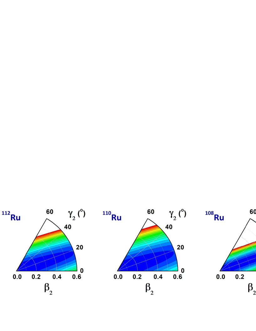
Figure 2: Collective potentials for ^108-112Ru calculated by Eq. (IV).

We have already mentioned that the mass parameters $B_{\beta\beta}$, $B_{\beta\gamma}$, and $B_{\gamma\gamma}$ are independent of the deformation $\beta_{2}$. Furthermore, their dependence on $\gamma_{2}$ is moderate, as can be seen in Fig. 3. With increasing $\gamma_{2}$, $B_{\beta\beta}$ increases and $B_{\gamma\gamma}$ decreases. One can observe that $B_{\beta\gamma}$ is much smaller than $B_{\beta\beta}$ and $B_{\gamma\gamma}$ for all three Ru isotopes, which implies that the coupling between $\beta_{2}$ and $\gamma_{2}$ is small. Once again, we should point out that the EFT formulation gives a different picture for collective energy spectra in comparisons to those of the 5DCH based on CDFT Chen et al. (2017).

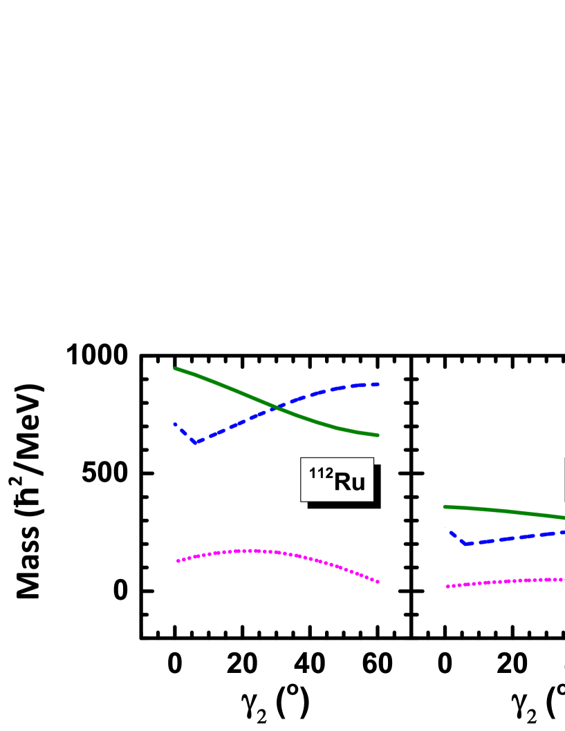
Figure 3: Mass parameters for ^108-112Ru calculated by Eq. (IV).

VI Summary

In summary, the EFT for triaxially deformed even-even nuclei has been generalized to include the vibrational degrees of freedom. The pertinent Lagrangian and Hamiltonian were obtained up to NLO. The LO Hamiltonian describes a set of uncoupled (anisotropic) harmonic oscillators. The NLO part couples rotations to vibrations, and it is found that the vibrations provide contributions to the angular momenta $I_{1}$, $I_{2}$, and $I_{3}$. This coupling makes the rotational Hamiltonian too complicated to be solved exactly.

Therefore, we have treated the NLO (rotational) Hamiltonian in first order perturbation theory. This leads to corrections from the vibrational motion in the form of so-called recoil term. For different vibrational states, the spin components of the bandhead become different and they depend on different vibrational quantum numbers.

The NLO Hamiltonian has also been expressed in terms of quadrupole deformation parameters $\beta_{2}$ and $\gamma_{2}$. A rotation-vibration Hamiltonian (without mutual coupling) is obtained. Its applicability has been examined in the description of the energy spectra of the ground state bands, $\gamma$-bands, and $K=4$ bands in ^108,110,112Ru isotopes. It is found that by taking into account the vibrational degree of freedom, the deviations for high-spin states in the $\gamma$-band, using the EFT with only rotational degree of freedom, disappear. This underlines the importance of including vibrational degrees of freedom in the EFT formulation.

The results presented in this work give us confidence to further generalize the EFT for triaxially deformed nuclei with odd mass number, which requires a systematic treatment of the coupling between the single particle motion and the collective rotational motion.

References

• Epelbaum (2006) E. Epelbaum, Prog. Part. Nucl. Phys. 57, 654 (2006).
• Epelbaum et al. (2009) E. Epelbaum, H.-W. Hammer, and U.-G. Meißner, Rev. Mod. Phys. 81, 1773 (2009).
• Machleidt and Entem (2011) R. Machleidt and D. R. Entem, Phys. Rep. 503, 1 (2011).
• Bertulani et al. (2002) C. Bertulani, H.-W. Hammer, and U. van Kolck, Nucl. Phys. A 712, 37 (2002).
• Hammer and Phillips (2011) H.-W. Hammer and D. Phillips, Nucl. Phys. A 865, 17 (2011).
• Ryberg et al. (2014) E. Ryberg, C. Forssén, H.-W. Hammer, and L. Platter, Phys. Rev. C 89, 014325 (2014).
• Bedaque and van Kolck (2002) P. F. Bedaque and U. van Kolck, Annu. Rev. Nucl. Part. Sci. 52, 339 (2002).
• Grießhammer et al. (2012) H. Grießhammer, J. McGovern, D. Phillips, and G. Feldman, Prog. Part. Nucl. Phys. 67, 841 (2012).
• Hammer et al. (2013) H.-W. Hammer, A. Nogga, and A. Schwenk, Rev. Mod. Phys. 85, 197 (2013).
• Papenbrock (2011) T. Papenbrock, Nucl. Phys. A 852, 36 (2011).
• Zhang and Papenbrock (2013) J. L. Zhang and T. Papenbrock, Phys. Rev. C 87, 034323 (2013).
• Papenbrock and Weidenmüller (2014) T. Papenbrock and H. A. Weidenmüller, Phys. Rev. C 89, 014334 (2014).
• Papenbrock and Weidenmüller (2015) T. Papenbrock and H. A. Weidenmüller, J. Phys. G: Nucl. Part. Phys. 42, 105103 (2015).
• Papenbrock and Weidenmüller (2016) T. Papenbrock and H. A. Weidenmüller, Phys. Scr. 91, 053004 (2016).
• Coello Pérez and Papenbrock (2015a) E. A. Coello Pérez and T. Papenbrock, Phys. Rev. C 92, 014323 (2015a).
• Coello Pérez and Papenbrock (2015b) E. A. Coello Pérez and T. Papenbrock, Phys. Rev. C 92, 064309 (2015b).
• Coello Pérez and Papenbrock (2016) E. A. Coello Pérez and T. Papenbrock, Phys. Rev. C 94, 054316 (2016).
• Bohr and Mottelson (1975) A. Bohr and B. R. Mottelson, Nuclear structure, vol. II (Benjamin, New York, 1975).
• Ring and Schuck (1980) P. Ring and P. Schuck, The nuclear many body problem (Springer Verlag, Berlin, 1980).
• Chen et al. (2017) Q. B. Chen, N. Kaiser, U.-G. Meißner, and J. Meng, Eur. Phys. J. A 53, 204 (2017).
• Bengtsson et al. (1984) R. Bengtsson, H. Frisk, F. May, and J. Pinston, Nucl. Phys. A 415, 189 (1984).
• Hamamoto and Sagawa (1988) I. Hamamoto and H. Sagawa, Phys. Lett. B 201, 415 (1988).
• Frauendorf and Meng (1997) S. Frauendorf and J. Meng, Nucl. Phys. A 617, 131 (1997).
• Meng et al. (2006) J. Meng, J. Peng, S. Q. Zhang, and S.-G. Zhou, Phys. Rev. C 73, 037303 (2006).
• Meng (2016) J. Meng, ed., Relativistic density functional for nuclear structure, vol. 10 of International Review of Nuclear Physics (World Scientific, Singapore, 2016).
• Coleman et al. (1969) S. Coleman, J. Wess, and B. Zumino, Phys. Rev. 177, 2239 (1969).
• Callan et al. (1969) C. G. Callan, S. Coleman, J. Wess, and B. Zumino, Phys. Rev. 177, 2247 (1969).
• Zhao et al. (2010) P. W. Zhao, Z. P. Li, J. M. Yao, and J. Meng, Phys. Rev. C 82, 054319 (2010).