Dark matter direct detection of a fermionic singlet at one loop

Abstract

The strong direct detection limits could be pointing to dark matter – nucleus scattering at loop level. We study in detail the prototype example of an electroweak singlet (Dirac or Majorana) dark matter fermion coupled to an extended dark sector, which is composed of a new fermion and a new scalar. Given the strong limits on colored particles from direct and indirect searches we assume that the fields of the new dark sector are color singlets. We outline the possible simplified models, including the well-motivated cases in which the extra scalar or fermion is a Standard Model particle, as well as the possible connection to neutrino masses. We compute the contributions to direct detection from the photon, the $Z$ and the Higgs penguins for arbitrary quantum numbers of the dark sector. Furthermore, we derive compact expressions in certain limits, i.e., when all new particles are heavier than the dark matter mass and when the fermion running in the loop is light, like a Standard Model lepton. We study in detail the predicted direct detection rate and how current and future direct detection limits constrain the model parameters. In case dark matter couples directly to Standard Model leptons we find an interesting interplay between lepton flavor violation, direct detection and the observed relic abundance.

1 Introduction

Direct detection (DD) experiments search for dark matter (DM) scatterings off nuclei in underground detectors. The current limits impose very strong constraints on the parameters of Weakly Interacting Massive Particles (WIMPs), which are one of the prototype DM candidates. The current most stringent DD limits for WIMPs in the mass range of $[10,1000]$ GeV come from xenon experiments [1, 2, 3]. In this work we hypothesize that the absence of DD signals may be reconciled with the WIMP paradigm by generating the scattering at one-loop order and thus with an extra $1/(16\pi^{2})^{2}$ suppression of the cross section. As we will see, current and next-generation experiments are able to test significant regions in parameter space of this class of scenarios.

There have been several works in the literature on DD at one-loop order. In Refs. [4, 5, 6, 7] the authors studied DD limits from photon interactions in the context of flavored DM and in Ref. [8] in the context of a radiative neutrino mass model (the scotogenic model [9]) with inelastic Majorana DM. In Ref. [10] the authors performed a detailed study of one-loop scenarios with a charged mediator directly coupled to Standard Model (SM) fields, including the $Z$ and Higgs boson contributions. For couplings to the first and second generation of quarks the dominant contribution may be due to scattering at tree level, while box diagrams may be significant for third generation quarks. Similarly, Ref. [11] studied direct detection of Majorana DM directly coupled to both left- and right-handed SM leptons via two charged scalar mediators. The $Z$ and Higgs contributions were also computed for the scotogenic model in Ref. [12] and also for DM connected to the SM via a neutrino-portal in Ref. [13]. In Ref. [14] the authors studied the one-loop contributions to DD in models with pseudo-scalar mediators or inelastic scattering. In the context of supersymmetry detailed computations have been performed for the bino [15] and wino [16, 17, 18] DM cases. In the latter scenario loop contributions to DM-nucleus scattering due to gauge bosons may give significant corrections.

In this work we study the DD scattering rate for the case of DM being a SM singlet Dirac or Majorana fermion $\psi$, which is coupled to a more complex dark sector. A conserved global U(1) or $Z_{2}$ symmetry is assumed in order to stabilize the DM particle. In our scenario there are no tree-level contributions to the DD cross section. The lowest order scattering off nuclei occurs at one-loop order via the penguin diagrams in Fig. 1, with a dark fermion $F$ and a dark scalar $S$ running in the loop. We assume that the new particles are color singlets, so that there are no flavor changing neutral currents in the quark sector, and there are only weak limits from direct production at the Large Hadron Collider (LHC). In this way box-diagram contributions to the scattering amplitude are absent. Our main goal is to study analytically the different contributions to the DM-nucleus scattering, as well as to outline possible simplified models, including those with SM fields. In addition we analyze the current limits from DD, as well as constraints coming from the relic abundance, lepton flavor violation (LFV) and anomalous magnetic dipole moments (AMMs).

Figure 1: One-loop penguin diagrams for fermionic singlet DM scattering off nuclei. They are generated with up to two heavy particles from a dark sector (a scalar $S$ and a fermion $F$). The photon and $Z$ boson are coupled to the new fermion (left diagram) or the new scalar (right diagram). For minimal models with one fermion the Higgs boson $h$ only couples to the scalar $S$, but SM fermions in the loop also lead to a Higgs penguin diagram where the SM Higgs boson is attached to the fermion line. The possible quantum numbers of the dark particles are given in Tab. 1.

The paper is structured as follows: In Sec. 2 we study the UV completions of the fermionic DM scenario including models with SM particles in the loop. In order to fix the notation we review in Sec. 3 the relevant effective operators for DD at the quark level and also their non-relativistic (NR) versions at the nucleon level. In Sec. 4 we derive analytical expressions for the Wilson coefficients and provide compact expressions in certain limits. In Sec. 5 we perform a numerical analysis of the phenomenology relevant for DD. First we show some numerical examples for the Wilson coefficients at the quark and nucleon level (the latter in their NR version). Afterwards we derive the current limits on the model parameters and discuss future expected sensitivity. We also discuss limits from LFV processes for models in which DM is directly coupled to SM leptons. Sections 4 and 5 contain the main results of this paper. We discuss other phenomenological aspects of the proposed scenario, such as the DM relic abundance, invisible decays and searches at colliders in Sec. 6. Finally we present our conclusions in Sec. 7.

The manuscript also includes several appendices with technical details. The generalization to larger symmetry groups in the dark sector is presented in App. A. In App. B we show a compact expression for the differential cross section in order to make contact with the literature and we briefly review the differential event rate for DD. In App. C we give generic expressions for Higgs and $Z$ boson invisible decays into DM. Relevant formulae for LFV observables and for AMMs of leptons are provided in App. D. Details about the calculation of the relic abundance are collected in App. E and the numerical expressions for the matching to NR operators are given in App. F.

Dark sector	Field	SU(3)C	SU(2)L	U(1)Y	U(1)dm
Dark matter	$\psi$	1	1	0	$1$
Dark scalar	$S$	1	$d_{F}$	$Y_{F}$	$q_{s}$
Dark fermion	$F$	1	$d_{F}$	$Y_{F}$	$q_{s}+1$

Table 1: Particle content and quantum numbers of the fermionic DM scenario with a dark fermion and a dark scalar. The dark sector is charged under a global U(1) symmetry which stabilizes the DM $\psi$.

2 Fermionic singlet dark matter

In the following sections we first present simplified models of Dirac and Majorana fermion DM with vector-like fermions in the loop and then discuss SM particles in the loop.

2.1 Dirac dark matter

The new particles can have different combinations of quantum numbers as displayed in Tab. 1. We consider a global U(1)_dm symmetry in the dark sector to stabilize DM. It can equally be replaced by a discrete $Z_{n}$ subgroup. Other symmetry groups are discussed in App. A.

The interaction Lagrangian for the fields $\psi$, $F$ and $S$ reads

$$\begin{split}\mathcal{L}_{\psi}=&\;i\,\overline{\psi}\,\not{\partial}\,\psi\,-\,m_{\psi}\,\overline{\psi}\,\psi\,+\,i\,\overline{F}\,\not{D}\,F\,-\,m_{F}\,\overline{F}\,F+\left(D_{\mu}S\right)^{\dagger}D^{\mu}S-\mathcal{V}(S,H)\\ &-\,\Big{(}y_{1}\,\overline{F_{\rm R}}\,S\,\psi_{\rm L}\,+y_{2}\,\overline{F_{\rm L}}\,S\,\psi_{\rm R}\,+\,\text{H.c.}\Big{)}\,,\end{split}$$ (1)

where $H$ is the SM Higgs doublet and $\mathcal{V}(S,H)$ denotes the scalar potential. The DM $\psi$ is a SM fermion singlet, but is charged under the dark sector symmetry. The fields $F$ and $S$ are charged under the electroweak gauge group. Electroweak gauge invariance requires them to be in the same SU(2)${}_{\text{L}}$ irreducible representation of dimension $d_{F}$ and to have equal hypercharge $Y_{F}$. Notice that in some cases there can be interactions with the SM fields which are subject to strong constraints. We discuss such cases in Sec. (2.3).

In the case of a global symmetry, even if DM is stable at the renormalizable level, higher-order Planck-scale suppressed operators may induce its decay [19]. In particular for a Dirac fermion $\psi$ the dimension-5 operator $\overline{\psi}{\tilde{H}}^{\dagger}(\not{D}L)$ with the SM lepton doublet $L$ is one such example. One can construct UV completions of such operators by softly-breaking the global symmetry in the dark sector which induces decays, possibly radiatively. The limits dramatically depend on the DM mass and the Wilson coefficient of the operator. For the rest of the paper we assume that DM is cosmologically stable and that it satisfies all indirect detection constraints on decaying DM.

In our simplified scenario with the interactions given in Eq. (1) it would seem that two of the three new states were stable: $\psi$ and one of $S$ or $F$. For the following discussion let us assume $m_{S}\geq m_{F}+m_{\psi}$ so that $F$ is potentially stable, while $S$ can decay. Then, there are two possibilities: (i) If the fermion $F$ is a SM singlet (but charged under the dark group), it also contributes to the DM relic density. Hence, the DD rate of the $\psi$ has to be rescaled by its smaller density under the assumption that the global density scales as the local one, and there is a similar DD rate for $F$ via Higgs penguins with $\psi$ in the loop. (ii) If $F$ is charged under the SM group (SU(2)${}_{\text{L}}$ charges and/or hypercharge) its electrically charged components have to decay given the stringent limits on charged stable particles [21, 22, 23, 24]. If the components of $F$ mix with SM leptons, they decay like in the model discussed in Refs. [25, 26]. Otherwise, as for the DM via the interaction $\overline{\psi}{\tilde{H}}^{\dagger}(\not{D}L)$, the fermion $F$ may also decay into SM particles via non-renormalizable operators, which are allowed on general grounds, unless $F$ carries fractional electric charge, or other symmetries forbid them. In this case the fermion $F$ has to decay much faster than the long-lived DM particle.

If $F$ is a SM lepton, a charged lepton or a neutrino, it may be stable. Similarly, if $F$ is a right-handed neutrino, it mixes with SM neutrinos and decay. Also, in the case in which $S$ is the SM Higgs doublet and $F$ a heavier fermion, the latter may decay into the SM Higgs boson. We discuss all these possibilities in more detail below.

In general the SM Higgs boson couples to the new scalar multiplet $S$ via a Higgs portal interaction in the scalar potential $\mathcal{V}(S,H)$. Depending on the quantum numbers of the particles in the dark sector, it may also have an interaction with the fermion $F$, for instance if the latter is a SM lepton. In the case of a charged lepton $\ell$ in the loop, the largest Higgs interactions are proportional to the square of its mass $(m_{\ell}/v)^{2}\ll 1$, with the electroweak vacuum expectation value (VEV) $v\simeq 246$ GeV. Therefore this contribution is suppressed and can be safely neglected. While these interactions are even further suppressed for Dirac neutrinos, in principle it is possible to have $\mathcal{O}(1)$ Yukawa couplings for Majorana neutrinos (we discuss this case in Sec. 2.3.3).

The Higgs portal contribution depends on the coupling of the SM Higgs boson $h$ to a pair of scalars $S$ after electroweak symmetry breaking. In the case of a complex scalar $S$, we parameterize it in terms of

$$\mathcal{V}(S,h)\;\supset\;\lambda_{HS}\,v\,h(S^{\dagger}S)$$ (2)

and similarly for a real scalar $S$ with an additional factor $1/2$ in order for the Feynman rule (and therefore the expression of the Wilson coefficients) to be identical

$$\mathcal{V}(S,h)\;\supset\;\frac{\lambda_{HS}v}{2}\,hS^{2}\,.$$ (3)

In the case of a complex scalar $S$, the Higgs couplings of Eq. (2) are induced by SM gauge invariant Higgs portal interactions such as

$$(H^{\dagger}H)(S^{\dagger}S) =hvS^{\dagger}S+\dots$$ (4)

$$(H^{\dagger}S)(S^{\dagger}H) =hv|S_{d}|^{2}+\dots,\qquad\qquad\mathrm{with}\;S_{d}\equiv(S_{d,r}+iS_{d,i})/\sqrt{2}\,.$$ (5)

$$(H^{\dagger}S)^{2}+\,\text{H.c.} =hv\left(S_{d,r}^{2}-S_{d,i}^{2}\right)+\dots$$ (6)

$$H^{\dagger}[\mathbf{S}^{\dagger},\mathbf{S}]H =hv(|S^{+}|^{2}-|S^{-}|^{2})+\dots$$ (7)

The term in the first line is always present, while those in the second and third lines require $S$ to be an SU(2)${}_{\text{L}}$ doublet, $S\equiv(S_{u},S_{d})^{T}$. Moreover the term in Eq. (6) assumes that $S$ has the same hypercharge as the SM Higgs doublet, which we write after spontaneous electroweak symmetry breaking as $H\equiv(0,(h+v)/\sqrt{2})^{T}$. Finally the term in the last line exists for electroweak triplets $\mathbf{S}\equiv S\cdot\sigma$, where $S^{\pm}$ denotes the coefficients of $\sigma^{\pm}$. In the following we parameterize all the results in terms of $\lambda_{HS}$, which allows to easily generalize the result of Higgs penguins for arbitrary combinations of Higgs portals. If $S^{\pm}$ ($S_{d,r}$ and $S_{d,i}$) have the same mass, their contribution from the interactions (5) and (6) to the DD scattering amplitude exactly cancels due to the relative minus sign in the interaction term. For equal masses the effective coupling $\lambda_{HS}$ can be generalized from the singlet case to an arbitrary SU(2)${}_{\text{L}}$ representation of dimension $d_{F}$ by replacing

$$\lambda_{HS}\to\begin{cases}2\,\lambda_{HS,1}+\lambda_{HS,2}&\text{if $d_{F}=2$}\\ d_{F}\,\lambda_{HS,1}&\text{otherwise}\end{cases}$$ (8)

where $\lambda_{HS,1}$ ($\lambda_{HS,2}$) is the coupling of the quartic scalar coupling in Eq. (4) (Eq. (5)).

Dark sector	Field	SU(3)C	SU(2)L	U(1)Y	$Z_{2}$
Dark matter	$\psi$	1	1	0	$-1$
Dark scalar	$S$	1	$d_{F}$	$Y_{F}$	$\pm 1$
Dark fermion	$F$	1	$d_{F}$	$Y_{F}$	$\mp 1$

Table 2: Particle content and quantum numbers of the Majorana DM scenario with a dark fermion and a dark scalar. The dark sector is charged under a $Z_{2}$ symmetry which stabilizes the DM $\psi$.

2.2 Majorana dark matter

If the DM particle is in a real representation of a stabilizing dark sector group, it could be a Majorana particle $\psi\equiv\psi_{L}+(\psi_{L})^{c}$ (keeping the 4-component notation). We consider the simplest case of a $Z_{2}$ symmetry in the dark sector and comment on the general case in App. A. The particle content for Majorana DM is listed in Tab. 2. The Lagrangian is given by

$$\begin{split}\mathcal{L}_{\psi}=&\;\frac{1}{2}\overline{\psi}\,(i\,\not{\partial}-m_{\psi})\,\psi\,+\,i\,\overline{F}\,\not{D}\,F\,-\,m_{F}\,\overline{F}\,F+\left(D_{\mu}S\right)^{\dagger}D^{\mu}S-\mathcal{V}(S,H)\\ &-\,\Big{(}y_{1}\,\overline{F_{\rm R}}\,S\,\psi\,+y_{2}\,\overline{F_{\rm L}}\,S\,\psi\,+\,\text{H.c.}\Big{)}\,.\end{split}$$ (9)

If additionally $Y_{F}=0$ and consequently $S$ and $F$ both transform according to a real representation, they can be chosen to be a real scalar and a Majorana fermion $F=F_{R}+(F_{R})^{c}$, respectively, and the fermionic part of the Lagrangian simplifies to

$$\mathcal{L}_{\psi}\;=\;\frac{1}{2}\overline{\psi}\,(i\,\not{\partial}-m_{\psi})\,\psi\,+\,\frac{1}{2}\,\overline{F}\,(i\not{\partial}-m_{F})\,F\,-\,\Big{(}y\,\overline{F}\,S\,\psi\,+\text{H.c.}\Big{)}$$ (10)

with $y=y_{1}=y_{2}$.

2.3 Standard Model particles in the loop

It is also interesting to study the case where one of the particles in the loop is a SM state. As either the scalar $S$ or the fermion $F$ need to be charged under the dark symmetry, only one of them can be substituted by a SM field. We discuss in the following the cases of $S$ being the Higgs doublet $H$, and $F$ being the lepton doublet $L$, the right-handed charged lepton $e_{R}$ or a right-handed neutrino $\nu_{R}$. Interestingly, these types of leptophilic models have some very nice features: (i) the absence of charged stable particles; (ii) the possibility to generate the correct relic abundance by annihilations into leptons; (iii) an interplay with LFV and leptonic AMMs; (iv) the possible relation to lepton number violation (LNV) and neutrino masses; (v) other possible phenomenological signals at future lepton colliders, like MET searches.

2.3.1 Left-handed lepton doublet

The quantum numbers of the remaining states are fixed by demanding that the fermion $F$ in the loop is the SM lepton doublet $L$, as can be seen in Tab. 3. Moreover $y_{1}=0$ in Eq. (1) for Dirac DM (or eq. (9) for Majorana DM), because we are now considering only chiral left-handed (LH) fermions.

Sector	Field	SU(3)C	SU(2)L	U(1)Y	$U(1)_{\rm dm}$
Dark matter	$\psi$	1	1	0	1
Dark scalar	$S$	1	2	$-1/2$	$-1$
SM lepton doublet	$L$	1	2	$-1/2$	0

Table 3: Particle content and quantum numbers of the dark fermion scenario with the SM lepton doublet $L$ and a dark scalar.

The coupling of the DM to the lepton doublets can lead to new contributions to LFV processes as well as AMMs of leptons, which are induced by loop diagrams with the dark scalar and the DM in the loop. These pose strong constraints on the flavor structure of the Yukawa couplings. However, the flavor constraints can be easily circumvented if DM only couples to the tau lepton.

In general, for direct couplings to leptons, it is possible to assign lepton number either to the DM particle $\psi$ or the scalar $S$. An example with Majorana fermion DM $\psi$ and a discrete $Z_{2}$ symmetry ($S\to-S$, $\psi\to-\psi$) is the well-known scotogenic model, proposed in Ref. [9] and extensively studied, e.g., in Refs. [28, 29, 30, 31, 32, 8, 33, 34, 35, 36, 37]. See also the recent review on radiative neutrino mass models [38]. In this case lepton number is broken by the combination of the Majorana mass term of $\psi$ and the operator in Eq. (6). These interactions generate neutrino masses and lepton mixing at one-loop order, which significantly constrain the parameter space of the model. However, in general DD and neutrino masses decouple, because the LNV coupling in the potential could be made arbitrarily small without affecting DD. For fermionic DM, typically, either coannihilations [20] or the freeze-in mechanism [39, 40] need to be invoked in order to be compatible with low energy constraints, specially the limit stemming from non-observation of $\mu\rightarrow e\gamma$.

2.3.2 Right-handed charged lepton

If $F$ is the SM right-handed (RH) charged lepton $e_{\rm R}$, the quantum numbers are fixed as shown in Tab. 4. In this case $y_{2}=0$ in Eq. (1) for Dirac DM (or eq. (9) for Majorana DM), because the fermions have RH chirality.

Sector	Field	SU(3)C	SU(2)L	U(1)Y	U(1)dm
Dark matter	$\psi$	1	1	0	$1$
Dark scalar	$S$	1	1	$-1$	$-1$
RH charged lepton	$e_{\rm R}$	1	1	$-1$	0

Table 4: Particle content and quantum numbers of the dark fermion scenario with the SM right-handed charged lepton $e_{\rm R}$ and a dark scalar.

As in the previous case one should expect new contributions to lepton AMMs and LFV processes. By demanding that the scalar singlet $S$ has lepton number $+1$, the total lepton number is conserved at the renormalizable level (the term in Eq. (6)) is absent) and consequently no Majorana neutrino masses are induced.

2.3.3 Right-handed neutrino

Dark matter may also couple to right-handed neutrinos $\nu_{\rm R}$ with $y_{2}=0$ in Eq. (1) for Dirac DM (or eq. (9) for Majorana DM). In this case the quantum numbers are fixed as shown in Tab. 5.

Sector	Field	SU(3)C	SU(2)L	U(1)Y	U(1)dm
Dark matter	$\psi$	1	1	0	$1$
Dark scalar	$S$	1	1	$\mathrm{𝟎}$	$-1$
RH neutrino	$\nu_{\rm R}$	1	1	$\mathrm{𝟎}$	0

Table 5: Particle content and quantum numbers of the dark fermion scenario with the SM right-handed neutrino $\nu_{\rm R}$ and a dark scalar.

As all particles in the loop are neutral, the only possible interactions are with the $Z$ and Higgs bosons via the mixing of left- and right-handed neutrinos. This mixing is induced after electroweak symmetry breaking by

$$\mathcal{L}_{\nu_{\rm R}}\;=\;-\overline{L}\,Y_{\nu}\,\nu_{\rm R}\,\tilde{H}\,-\frac{1}{2}\,\overline{\nu}_{\rm R}M_{\rm R}\nu_{\rm R}^{c}\,+{\rm H.c.}\,.$$ (11)

In this scenario there are two possibilities regarding the nature of neutrinos: they are Dirac fermions for $M_{\rm R}=0$, or Majorana fermions for $M_{\rm R}\neq 0$. In the latter case, Majorana masses for the active light neutrinos are generated via the seesaw mechanism. In the seesaw scenario the active-sterile mixing angles are tiny, either due to small Yukawa couplings or large right-handed Majorana neutrino masses, and thus the $Z$ penguin contributions and the additional Higgs penguin contributions are extremely small, which agrees with Eq. (19) of Ref. [13]. A possible way-out is to consider an inverse-seesaw scenario, where the suppression needed to have small neutrino masses originates from a small LNV Majorana mass term, and not from small Yukawa couplings and/or large right-handed Majorana masses.

As DM couples to the SM particles mainly via neutrinos, this is known as the neutrino portal. It has been studied in detail for general heavy SM singlet Dirac and Majorana fermions $\nu_{R}$ in Ref. [13] and also in Refs. [41, 42].

2.3.4 Higgs doublet

Finally we consider the case of $S$ being the SM Higgs. This fixes the SM quantum numbers of the new particles, which are shown in Tab. 6.

Sector	Field	SU(3)C	SU(2)L	U(1)Y	U(1)dm
Dark matter	$\psi$	1	1	0	1
SM Higgs doublet	$H$	1	2	$1/2$	0
Dark fermion	$F$	1	2	$1/2$	1

Table 6: Particle content and quantum numbers of the DM fermion scenario with the SM Higgs and a dark fermion.

This case is qualitatively different, because the neutral component of the electroweak doublet $F$ and the fermion field $\psi$ mix after electroweak symmetry breaking. The lighter of the two neutral mass eigenstates is the DM particle. The Yukawa interactions with the Higgs necessarily induces tree-level contributions to DD via Higgs and $Z$ boson exchange. Although a tree-level contribution exists, DD may still be dominated by the loop-level induced electric or magnetic dipole moments, because they are long-range interactions.

3 Effective operators for dark matter direct detection

In the following sections we briefly review the effective operators for DM DD. In Sec. 3.1 we show those involving DM interactions with quarks, while in Sec. 3.2 we briefly discuss their NR versions at the nucleon level.

3.1 Wilson coefficients at the quark level

Here we review the necessary notation for the effective interactions of the DM with the quarks. The effective Lagrangian at the quark level for a DM fermion $\psi$ is

$$\mathcal{L}_{\rm eff}\;=\;\sum_{k,q}\,c_{k}^{q}\,\mathcal{O}_{k}^{q}+c_{g}\,\mathcal{O}_{g}+\tilde{c}_{g}\,\tilde{\mathcal{O}}_{g}+\mu_{\psi}\mathcal{O}_{\text{mag}}+d_{\psi}\mathcal{O}_{\text{edm}}\,,$$ (12)

where $c_{k}^{q}$ are the dimensionful Wilson coefficients with the quark $q$, $c_{g}$ and $\tilde{c}_{g}$ are the Wilson coefficients for gluon operators and $\mu_{\psi}$ and $d_{\psi}$ magnetic and electric dipole moments. We implicitly assume that the operators are generated at a scale above the nuclear scale, $\sim 2$ GeV. See App. F for further details.

We focus on the contributions to spin-independent (SI) and spin-dependent (SD) operators of photon, $Z$ boson and Higgs penguins which are not momentum or velocity suppressed. The latter would yield very small rates, as there is already the one-loop squared factor at cross section level, $1/(16\pi^{2})^{2}$. We start the discussion with the case of $\psi$ being a Dirac fermion and later on discuss the case of DM being a Majorana particle.

For SI scattering the relevant dimension-6 effective operators are

$$\mathcal{O}^{q}_{\text{SS}}=m_{q}(\overline{\psi}\psi)(\overline{q}q),\qquad\qquad\mathcal{O}^{q}_{\text{VV}}=(\overline{\psi}\gamma^{\mu}\psi)(\overline{q}\gamma_{\mu}q)\,,$$ (13)

where $q$ denotes the quark field. $\mathcal{O}^{q}_{\text{SS}}$ is generated by the gauge-invariant dimension-7 operators $(\overline{\psi}\psi)(\overline{Q}_{L}\tilde{H}u_{R})$ and $(\overline{\psi}\psi)(\overline{Q}_{L}Hd_{R})$, where $Q_{L},\,u_{R},\,d_{R}$ represent the quark flavor eigenstates. $\mathcal{O}^{q}_{\text{SS}}$ flips chirality and it is generated by Higgs exchange and thus we factor out the quark mass $m_{q}$. $\mathcal{O}^{q}_{\text{VV}}$ preserves chirality and is generated by photon or $Z$ exchange. The contribution from the photon penguin can be related to the anapole moment $\overline{\psi}\gamma^{\mu}\psi\,\partial^{\nu}F_{\mu\nu}$ and the (non-gauge invariant) milli-charge operator $\overline{\psi}\gamma^{\mu}\psi\,A_{\mu}$ via the equations of motion for the photon.

There are also scatterings of the DM with gluons at two-loop order which generate the dimension-7 operators:

$$\mathcal{O}_{g}=\frac{\alpha_{s}}{12\pi}(\overline{\psi}\psi)G^{a\mu\nu}G^{a}_{\mu\nu},\qquad\qquad\tilde{\mathcal{O}}_{g}=\frac{\alpha_{s}}{8\pi}(\overline{\psi}\psi)G^{a\mu\nu}\tilde{G}^{a}_{\mu\nu}\,,$$ (14)

where $a=1,...,8$ are the adjoint color indices, $\alpha_{s}$ is the strong coupling constant, $G_{\mu\nu}$ the gluon field strength tensor and $\tilde{G}_{\mu\nu}\equiv\tfrac{1}{2}\epsilon_{\mu\nu\rho\sigma}G^{\rho\sigma}$ its dual. $\mathcal{O}_{g}$ is induced from $\mathcal{O}_{SS}^{q}$ after integrating out the heavy quarks. We explicitly factorized out a loop factor, as these operators can never be generated at tree level.

For SD interactions the relevant dimension-6 effective operators are

$$\mathcal{O}_{\text{AA}}^{q}=(\overline{\psi}\gamma^{\mu}\gamma_{5}\psi)(\overline{q}\gamma_{\mu}\gamma_{5}q),\qquad\qquad\mathcal{O}^{q}_{\rm TT}=(\overline{\psi}\sigma^{\mu\nu}\psi)(\overline{q}\sigma_{\mu\nu}q)\,,$$ (15)

where $\sigma_{\mu\nu}=\tfrac{i}{2}[\gamma_{\mu},\gamma_{\nu}]$. Only the $Z$ boson contributes to $\mathcal{O}^{q}_{\text{AA}}$. In SM effective theory the tensor operator may arise from one of the dimension-7 operators $(\overline{\psi}\sigma^{\mu\nu}\psi)(\overline{Q}_{L}\tilde{H}\sigma_{\mu\nu}u_{R})$ and $(\overline{\psi}\sigma^{\mu\nu}\psi)(\overline{Q}_{L}H\sigma_{\mu\nu}d_{R})$ which are however not induced at leading order.

Photon penguins also generate long-range interactions which are described by the magnetic (CP-even) and electric (CP-odd) dipole moments of the DM $\psi$, namely

$$\mathcal{O}_{\rm mag}=\frac{e}{8\pi^{2}}(\overline{\psi}\sigma^{\mu\nu}\psi)F_{\mu\nu},\qquad\qquad\mathcal{O}_{\rm edm}=\frac{e}{8\pi^{2}}(\overline{\psi}\sigma^{\mu\nu}i\gamma_{5}\psi)F_{\mu\nu}\,,$$ (16)

with $\mu_{\psi}$ and $d_{\psi}$ the coefficients of the magnetic and electric dipole moment operators introduced in Eq. (12), respectively. The latter are generated radiatively and therefore it is convenient to factorize a loop factor.

In the case of a Majorana DM particle there are only operators with the bilinears $\overline{\psi}\psi$, $\overline{\psi}\,\gamma_{5}\psi$ and $\overline{\psi}\,\gamma^{\mu}\gamma_{5}\psi$, so that the vector $\mathcal{O}^{q}_{\rm VV}$, the tensor $\mathcal{O}^{q}_{\rm TT}$ and the dipole moment operators, $\mathcal{O}_{\rm mag}$ and $\mathcal{O}_{\rm edm}$, vanish identically. Thus, for SI scattering only the Higgs penguin which generates $\mathcal{O}^{q}_{\rm SS}$ is present. For SD scattering $\mathcal{O}^{q}_{\rm AA}$ generated by the $Z$ boson can also be non-vanishing. In this case we also compute the photonic contribution to the anapole operator

$$\mathcal{O}^{q}_{\rm AV}=(\overline{\psi}\gamma^{\mu}\gamma_{5}\psi)(\overline{q}\gamma_{\mu}q)\,,$$ (17)

which gives rise to momentum-suppressed and velocity-suppressed NR operators (both SI and SD). See also Ref. [44] for a study of the phenomenology of Majorana DM in EFT.

In general the penguin contributions are isospin-violating, i.e., with different couplings to protons and neutrons ($f_{n}\neq f_{p}$). This isospin violation is maximal for photon contributions which only couple to protons. The latter dominate the DM-nucleus scattering via the dipole moments $\mu_{\psi}$ and $d_{\psi}$. Hence for SI DM-nucleus scattering the enhancement due to coherent scattering is $Z^{2}$ instead of $A^{2}$, with $Z$ ($A$) being the number of protons (nucleons) of the nucleus.

3.2 Non-relativistic Wilson coefficients at the nucleon level

The previous Wilson coefficients at the quark level generate non-trivial Wilson coefficients at the nucleon level [45, 46, 47]. The different contributions generally interfere. The matrix elements of DM-nucleon scattering can be written as a linear combination of the following relevant NR operators

$$\mathcal{O}_{1}^{N} =I_{\psi}I_{N} \mathcal{O}_{4}^{N} =\vec{S}_{\psi}\cdot\vec{S}_{N}$$ (18)

$$\mathcal{O}_{5}^{N} =\vec{S}_{\psi}\cdot\left(\vec{v}_{\perp}\times\frac{i\vec{q}}{m_{N}}\right)I_{N} \mathcal{O}_{6}^{N} =\left(\vec{S}_{\psi}\cdot\frac{\vec{q}}{m_{N}}\right)\left(\vec{S}_{N}\cdot\frac{\vec{q}}{m_{N}}\right)$$ (19)

$$\mathcal{O}_{8}^{N} =\left(\vec{S}_{\psi}\cdot\vec{v}_{\perp}\right)I_{N} \mathcal{O}_{9}^{N} =\vec{S}_{\psi}\cdot\left(\frac{i\vec{q}}{m_{N}}\times\vec{S}_{N}\right)$$ (20)

$$\mathcal{O}_{11}^{N} =-\left(\vec{S}_{\psi}\cdot\frac{i\vec{q}}{m_{N}}\right)I_{N}$$ (21)

in the convention of Ref. [48]. $I_{\psi}$ ($I_{N}$) denotes the identity operators for DM (nucleons), $\vec{S}_{\psi}$ ($\vec{S}_{N}$) denotes DM (nucleon) spin, and $\vec{q}$ and $\vec{v}_{\perp}$ describe the momentum and velocity exchange. We use DirectDM [48] to match the simplified models onto the NR operators. The numerical expressions for the matching to NR operators are collected in App. F. The NR Wilson coefficients may depend on the transferred momentum $\vec{q}$. Note the different normalizations of the spinors and the effective operators between Refs. [45, 46, 47, 49] and Refs. [50, 51, 52, 48]. In addition to the different definitions of the quark- and nucleon-level operators, in order to translate between these conventions one needs to multiply the NR Wilson coefficients of Refs. [50, 51, 52, 48] by $4\,m_{\psi}m_{N}$ ($4\,m_{\psi}|\vec{q}|^{2}$) in the case of contact (long-range) interactions. Further details can be found in the recent Refs. [49, 50, 51, 52, 48]. The differential cross section for DM scattering off nuclei is given in App. B.

4 Analytical results

The effective operators in Eq. (12) are generated at one-loop order from penguin diagrams mediated by the photon and the $Z$ and Higgs bosons. We have computed the different contributions using the Mathematica packages FeynRules [53], FeynArts [54], FormCalc and LoopTools [55, 56, 57], ANT [58] and Package X [59, 60]. As we show below, although the long-range interactions are expected to dominate, the short-range effective operators become relevant in some cases. One obvious example is DM-nucleus scattering of Majorana DM, since the dipole moments vanish. Therefore we show below all relevant contributions.

The interesting SI (SD) interactions in Eq. (12) are given by the dipole moment operators $\mathcal{O}_{\text{mag}}$ and $\mathcal{O}_{\text{edm}}$ as well as the operators $\mathcal{O}^{q}_{\rm SS}$, $\mathcal{O}_{g}$ and $\mathcal{O}^{q}_{\rm VV}$ ($\mathcal{O}^{q}_{\rm AA}$). All the other operators in Eq. (12) are suppressed in the limit of small momentum transfer by a factor $|\vec{q}|^{2}/m_{N}^{2}$ or $|\vec{q}|^{2}/m_{\psi}^{2}$, where $m_{N}$ is the nucleon mass. In the following we express the SI and SD Wilson coefficients in Eq. (12) in terms of the ratios

$$x_{\psi}\;\equiv\;\frac{m_{\psi}}{m_{S}}\quad\quad\text{and}\quad\quad x_{F}\;=\;\frac{m_{F}}{m_{S}}\,,$$ (22)

and the loop function

$$g\big{(}x_{\psi},x_{F}\big{)}\;=\;\frac{\ln\Bigg{(}\frac{1-x_{\psi}^{2}+x_{F}^{2}+\sqrt{x_{\psi}^{4}+(1-x_{F}^{2})^{2}-2x_{\psi}^{2}(1+x_{F}^{2})}}{2x_{F}}\Bigg{)}}{\sqrt{x_{\psi}^{4}+(1-x_{F}^{2})^{2}-2x_{\psi}^{2}(1+x_{F}^{2})}}\,.$$ (23)

It is convenient to define the vector and axial Yukawa couplings:

$$y_{V}\;\equiv\;\frac{1}{2}\left(y_{1}+y_{2}\right)\,,\quad\quad y_{A}\;\equiv\;\frac{1}{2}\left(y_{2}-y_{1}\right)\,.$$ (24)

Similarly, the interaction of the fermion $F$ with the $Z$ boson in Eq. (1) may be written in terms of vector and axial-vector couplings, namely

$$\mathcal{L}_{F}^{Z}\;=\;\frac{e}{c_{w}\,s_{w}}\,Z^{\mu}\,\overline{F}\,\gamma_{\mu}\left(z_{V}-z_{A}\,\gamma_{5}\right)F\,,$$ (25)

where $e>0$ is the proton electric charge, and $s_{w}\,(c_{w})$ denotes the sine (cosine) of the weak mixing angle. If $F$ is a vector-like fermion, then we have

$$z_{V}\;=\;c_{w}^{2}\,Q-Y_{F}\,,\quad\quad\quad z_{A}\;=\;0\,,$$ (26)

where $Q$ is the electric charge of the (component of the) field $F$, in units of $e$, and $Y_{F}$ is the corresponding hypercharge. Conversely, for a SM lepton $F$ we have

$$z_{V}\;=\;\frac{1}{2}\left((1-2s_{w}^{2})\,Q-Y_{F}\right)\,,\quad\quad\quad z_{A}\;=\;\frac{1}{2}\left(Q-Y_{F}\right)\,,$$ (27)

and the Yukawa couplings are

$$\begin{split}y_{V}&=\;y_{A}\;=\;\frac{y_{2}}{2}\quad\quad\quad\,\;\;\;\text{if $S$ is a doublet of SU(2)${}_{\text{L}}$}\,,\\ y_{V}&=\;-\,y_{A}\;=\;\frac{y_{1}}{2}\quad\quad\quad\,\text{if $S$ is a singlet of SU(2)${}_{\text{L}}$}\,.\end{split}$$ (28)

For simplicity of notation we report the full analytic results for SU(2)_L singlets $F$ and $S$. In the case of no mass splittings between the components of the SU(2)_L multiplets of dimension $d_{F}$ it is straightforward to generalize the results: The expressions for photon penguins and electric and magnetic dipole moments are generalized by replacing $Q\to d_{F}\,Y_{F}$. Higgs penguins are generalized for different scalar multiplets as in Eq. (8).

Most $Z$ penguin contributions (apart from some with chiral SM fermions) vanish at leading order. This is also the case for other SU(2)_L multiplets.

We summarize below the relevant contributions to the (Dirac or Majorana) DM–quark scattering amplitude. We have checked that our expressions agree with those reported in the literature in the appropriate limits: dipole and anapole moments in Refs. [5, 6, 8, 10], and also for the $Z$ boson contributions in Refs. [15, 10].

4.1 Dirac dark matter

The leading contributions for Dirac fermion DM are from dipole moments, the operators $\mathcal{O}_{VV}^{q}$ and $\mathcal{O}_{AA}^{q}$, and the scalar operator $\mathcal{O}_{SS}^{q}$. Integrating out heavy quarks induces the gluon operator $\mathcal{O}_{g}$.

4.1.1 Electromagnetic dipole moments

The magnetic and electric dipole moments are given by

$$\begin{split}\mu_{\psi}=&\;-\frac{Q}{4\,x_{\psi}^{3}\,m_{S}}\,\left|y_{V}\right|^{2}\Bigg{[}x_{\psi}^{2}+\left(1-x_{\psi}x_{F}-x_{F}^{2}\right)\ln x_{F}\\ &\;-\,\Big{(}x_{\psi}^{3}x_{F}-(1-x_{F}^{2})^{2}+x_{\psi}^{2}(1+x_{F}^{2})+x_{\psi}x_{F}(1-x_{F}^{2})\Big{)}g\big{(}x_{\psi},x_{F}\big{)}\Bigg{]}\\ &\;-\,\big{(}y_{V}\to y_{A},\,x_{\psi}\to-x_{\psi},\,x_{F}\to x_{F}\big{)}\,,\end{split}$$ (29)

and

$$\begin{split}d_{\psi}=&\;-\frac{Q}{2\,x_{\psi}^{2}\,m_{S}}\,\text{Im}[y_{V}\,y_{A}^{*}]\,x_{F}\Bigg{[}\ln x_{F}+\Big{(}1+x_{\psi}^{2}-x_{F}^{2}\Big{)}g\big{(}x_{\psi},x_{F}\big{)}\Bigg{]}\,.\end{split}$$ (30)

Both $\mathcal{O}_{\rm mag}$ and $\mathcal{O}_{\rm edm}$ flip chirality and therefore the dominant contributions to their coefficients are proportional to the heaviest fermion mass, either $m_{\psi}$ or $m_{F}$. In the limit $m_{\psi}\ll m_{F}<m_{S}$ these expressions reduce to

$$\mu_{\psi} \approx -\frac{Q}{4\,m_{S}}\left(\left|y_{V}\right|^{2}-\left|y_{A}\right|^{2}\right)x_{F}\,\frac{1-x_{F}^{2}+2\,\ln x_{F}}{(1-x_{F}^{2})^{2}}$$ (31)

$$+\frac{Q}{8\,m_{S}}\left(\left|y_{V}\right|^{2}+\left|y_{A}\right|^{2}\right)x_{\psi}\frac{1-x_{F}^{2}(x_{F}^{2}-4\ln x_{F})}{(1-x_{F}^{2})^{3}}\,,$$

$$d_{\psi} \approx -\frac{Q}{2\,m_{S}}\,\text{Im}[y_{V}^{*}\,y_{A}]\,x_{F}\,\frac{1-x_{F}^{2}+2\,\ln x_{F}}{(1-x_{F}^{2})^{2}}\,.$$ (32)

4.1.2 Photon penguin

Photon penguins induce the operator $\mathcal{O}_{VV}^{q}$. The relevant Wilson coefficient in the effective Lagrangian (12) is

$$\begin{split}c^{q}_{\rm VV}=&\;-\frac{\alpha_{\rm em}}{24\,\pi\,x_{\psi}^{4}}\,\frac{1}{m_{S}^{2}}\,Q\,Q_{q}\,\left|y_{V}\right|^{2}\\ &\;\Bigg{[}\Big{(}-3x_{\psi}^{6}+6x_{\psi}^{5}x_{F}+12x_{\psi}x_{F}(1-x_{F}^{2})^{2}+8(1-x_{F}^{2})^{3}+2x_{\psi}^{4}(5+x_{F}^{2})\\ &\;-6x_{\psi}^{3}x_{F}(1+3x_{F}^{2})-3x_{\psi}^{2}(5-2x_{F}^{2}-3x_{F}^{4})\Big{)}\frac{g\big{(}x_{\psi},x_{F}\big{)}}{1-(x_{\psi}-x_{F})^{2}}\\ &\;+\frac{2x_{\psi}^{2}(4-3x_{\psi}^{2}+6x_{\psi}x_{F}-4x_{F}^{2})}{1-(x_{\psi}-x_{F})^{2}}+(8+x_{\psi}^{2}-4x_{\psi}x_{F}-8x_{F}^{2})\ln x_{F}\Bigg{]}\\ &\;+\big{(}y_{V}\to y_{A},\,x_{\psi}\to-x_{\psi},\,x_{F}\to x_{F}\big{)}\,,\end{split}$$ (33)

where $Q_{q}$ is the electric charge of the quark $q$ in units of $e>0$. In the limit $m_{\psi}\ll m_{F}<m_{S}$ the expression above reduces to

$$c^{q}_{\rm VV}\;\approx\;\frac{Q\,Q_{q}\,\alpha_{\rm em}}{24\,\pi\,m_{S}^{2}}\,\big{(}\left|y_{V}\right|^{2}+\left|y_{A}\right|^{2}\big{)}\,\frac{3-3\,x_{F}^{2}+2\,(2+x_{F}^{2})\ln x_{F}}{(1-x_{F}^{2})^{2}}\,.$$ (34)

In the case the mass of the fermion in the loop is much smaller than the momentum transfer, $m_{F}\ll\sqrt{-q^{2}}$, we have

$$\begin{split}c^{q}_{\rm VV}\approx&\;\frac{Q\,Q_{q}\,\alpha_{\rm em}}{72\,\pi\,m_{S}^{2}}\,\big{(}\left|y_{V}\right|^{2}+\left|y_{A}\right|^{2}\big{)}\\ \,&\;\Bigg{[}\frac{12x_{\psi}^{4}\ln x_{q}-8x_{\psi}^{2}(3-x_{\psi}^{2})-3(8-7x_{\psi}^{2}+3x_{\psi}^{4})\ln\big{(}1-x_{\psi}^{2}\big{)}}{x_{\psi}^{4}(1-x_{\psi}^{2})}\Bigg{]}\end{split}$$ (35)

with $x_{q}\equiv\sqrt{-q^{2}/m_{S}^{2}}$.

4.1.3 $Z$ penguin

For a vector-like fermion the resulting SI and SD scattering amplitudes are suppressed by $|\vec{q}|^{2}/m_{F}^{2}$ and $|\vec{q}|^{2}/m_{S}^{2}$ due to a cancellation between the diagrams where the $Z$ boson couples to the scalar and to the fermion. Therefore, no strong constraints on the model parameters can be obtained. For SM leptons in the loop we distinguish two cases:

(i) If $S$ is a singlet under SU(2)_L, the axial-vector coupling in Eq. (27) is $z_{A}=0$ and both SI and SD scattering amplitudes are suppressed as for a vector-like fermion.

(ii) If $S\equiv(S^{0},S^{-})^{T}$ is a doublet under SU(2)_L, there are contributions from both diagrams where the $Z$ boson is attached to the SM lepton or the scalar in the loop

$$c^{q}_{\rm VV} = \sum_{f=\{\ell,\nu\}}\frac{(1+2\,Q_{f})\alpha_{\rm em}}{16\,\pi\,c_{w}\,s_{w}\,m_{Z}^{2}}\frac{q_{V}}{e}\,\frac{x_{f}^{2}}{x_{\psi}^{2}}\,\left|y_{2}\right|^{2}\bigg{[}\left(x_{f}^{2}-1-x_{\psi}^{2}\right)g\left(x_{\psi},x_{f}\right)-\ln x_{f}\bigg{]}\,,$$ (36)

$$c^{q}_{\rm AA} = \;c^{q}_{\rm VV}\,(q_{V}\rightarrow q_{A})\,.$$ (37)

The couplings $q_{V,A}$ are $q_{V}/e=3-8s_{w}^{2}/(12c_{w}s_{w})$ and $q_{A}/e=-1/(4c_{w}s_{w})$ for up-type quarks and $q_{V}/e=-3+4s_{w}^{2}/(12c_{w}s_{w})$ and $q_{A}/e=1/(4c_{w}s_{w})$ for down-type quarks. $Q_{f}$ denotes the electric charge of the lepton. We define $x_{\psi}\equiv m_{\psi}/m_{S^{-}}$, $x_{\ell}\equiv m_{\ell}/m_{S^{-}}$ and $x_{\nu}\equiv m_{\nu}/m_{S^{0}}$ with the charged lepton mass $m_{\ell}$ and the neutrino mass $m_{\nu}$. This agrees with the expression in Ref. [10]. The contribution with light active neutrinos in the loop is negligible because it is proportional to $x_{\nu}^{2}$ and thus the contribution is entirely determined by the charged lepton in the loop. However, for models with a neutrino portal as outlined in Sec. 2.3.3 there may be a sizable contribution from right-handed neutrinos (mixed with left-handed neutrinos) in the loop. In the limit of small DM mass, $x_{\psi}\ll 1$, the contribution of right-handed neutrinos is

$$c_{{\rm VV},N}^{q} =\frac{\alpha_{\rm em}\,\sin^{2}\theta}{16\pi c_{w}s_{w}m_{Z}^{2}}\frac{q_{V}}{e}|y_{2}|^{2}\frac{x_{N}^{2}}{(1-x_{N}^{2})^{2}}\left(1-x_{N}^{2}+2\ln x_{N}\right)$$ (38)

$$c_{{\rm AA},N}^{q} =c_{{\rm VV},N}^{q}(q_{V}\to q_{A})$$ (39)

with the active-sterile mixing angle $\theta$. We define $x_{N}\equiv m_{N}/m_{S}$ with the heavy neutrino mass $m_{N}$. These interactions are also discussed in Ref. [13] (see also Ref. [61]). In the case of mixing of vector-like charged fermions with SM charged leptons, there is an overall minus sign in the expressions of Eqs. (38) and (39).

4.1.4 Higgs penguin

At leading order in $|\vec{q}|^{2}$ there is only the contribution to the SI scattering amplitude. The relevant Wilson coefficient generated by the Higgs-portal interaction is

$$\begin{split}c^{q}_{\rm SS}=&\;-\frac{\lambda_{HS}}{16\,\pi^{2}\,x_{\psi}^{3}\,m_{h}^{2}}\,\frac{1}{m_{S}}\,\left|y_{V}\right|^{2}\Bigg{[}x_{\psi}^{2}+\left(1-x_{\psi}^{2}-x_{\psi}x_{F}-x_{F}^{2}\right)\ln x_{F}\\ &\;+\left(1-x_{\psi}^{2}-2x_{\psi}x_{F}-x_{F}^{2}\right)\left(1-x_{\psi}^{2}+x_{\psi}x_{F}-x_{F}^{2}\right)g\left(x_{\psi},x_{F}\right)\Bigg{]}\\ &\;-\,\big{(}y_{V}\to y_{A},\,x_{\psi}\to-x_{\psi},\,x_{F}\to x_{F}\big{)}\,.\end{split}$$ (40)

As previously mentioned we neglect the contribution from the Higgs penguin where the Higgs boson couples to a SM lepton in the loop, because it is suppressed by $(m_{\ell}/v)^{2}\ll 1$. As in the case of $\mathcal{O}_{\rm mag}$ and $\mathcal{O}_{\rm edm}$, the operator $\mathcal{O}_{SS}^{q}$ flips chirality, and therefore the dominant contribution to its Wilson coefficients is proportional to either $m_{\psi}$ or $m_{F}$. If both $F$ and $\psi$ are charged under U(1)_dm, then $m_{\psi}<m_{F}$ and thus the largest contribution comes with the chirality flip on the fermion line of $F$. On the contrary if $F$ is a SM lepton the largest Higgs contribution is proportional to $m_{\psi}$. In the limit $m_{\psi}\ll m_{F}<m_{S}$, Eq. (40) simplifies to

$$\begin{split}c^{q}_{\rm SS}\approx&\;-\frac{\lambda_{HS}}{16\,\pi^{2}\,m_{h}^{2}\,m_{S}\,(x_{F}^{2}-1)^{2}}\,\Bigg{\{}x_{F}\,(\left|y_{V}\right|^{2}-\left|y_{A}\right|^{2})\,\left(-x_{F}^{2}+2\,x_{F}^{2}\,\ln\left(x_{F}\right)+1\right)+\\ &\;+\frac{x_{\psi}}{2\,(x_{F}^{2}-1)}\,(\left|y_{V}\right|^{2}+\left|y_{A}\right|^{2})\,\left(-3\,x_{F}^{4}+4\,x_{F}^{4}\,\ln\left(x_{F}\right)+4\,x_{F}^{2}-1\right)\Bigg{\}}\,.\end{split}$$ (41)

4.2 Majorana dark matter

4.2.1 Photon penguin

For Majorana DM $\psi$ the electromagnetic dipole moments identically vanish and the only allowed electromagnetic form factor is the anapole moment. This gives rise to the effective operator $\mathcal{O}^{q}_{\rm AV}$ in Eq. (17). We obtain

$$c^{q}_{\rm AV}\;=\;-\frac{Q\,Q_{q}\,\alpha_{\rm em}}{2\,\pi\,x_{\psi}^{2}\,m_{S}^{2}}\,\text{Re}[y_{V}^{*}\,y_{A}]\,\Bigg{[}\ln x_{F}+\left(1+\frac{x_{\psi}^{2}}{3}-x_{F}^{2}\right)g\left(x_{\psi},x_{F}\right)\Bigg{]}\,.$$ (42)

In the limit $m_{\psi}\ll m_{F}<m_{S}$ this simplifies to

$$c^{q}_{\rm AV}\;\approx\;\frac{Q\,Q_{q}\,\alpha_{\rm em}}{6\,\pi\,m_{S}^{2}}\,\text{Re}[y_{V}^{*}\,y_{A}]\,\ \frac{3-3\,x_{F}^{2}+2\,(2+x_{F}^{2})\ln x_{F}}{(1-x_{F}^{2})^{2}}\,.$$ (43)

In the case the mass of the fermion in the loop is much smaller than the momentum transfer, $m_{F}\ll\sqrt{-q^{2}}$, we have

$$\begin{split}c^{q}_{\rm AV}=&\;-\frac{Q\,Q_{q}\,\alpha_{\rm em}}{18\,\pi\,m_{S}^{2}}\,\text{Re}[y_{V}^{*}\,y_{A}]\,\frac{2x_{\psi}^{2}(5-6\ln x_{q})+3(3+x_{\psi}^{2})\ln\big{(}1-x_{\psi}^{2}\big{)}}{x_{\psi}^{2}(1-x_{\psi}^{2})}\,,\end{split}$$ (44)

where $x_{q}\equiv\sqrt{-q^{2}/m_{S}^{2}}$.

4.2.2 $Z$ and Higgs penguin

For a vector-like fermion $F$ in the loop the $Z$ penguin diagram does not contribute to the SI scattering amplitude, because the DM vector current identically vanishes for Majorana fermions. The SD scattering amplitude is suppressed by $|\vec{q}|^{2}/m_{F}^{2}$ and $|\vec{q}|^{2}/m_{S}^{2}$ due to a cancellation similar to that occurring in the case of Dirac fermion DM, see Sec. 4.1.3. If $F$ is a left-handed lepton doublet, and consequently $S\equiv(S^{0},S^{-})^{T}$ is an SU(2)_L doublet, we find at leading order in $|\vec{q}|^{2}$: $c^{q}_{\rm VV}=0$ and $c^{q}_{\rm AA}$ is a factor of two larger than result for the Dirac case provided in Eq. (37). If $F$ is a right-handed charged lepton or a right-handed neutrino, the scalar $S$ is necessarily an SU(2)_L-singlet and thus the axial-vector coupling $z_{A}$ in Eq. (27) is zero and both SI and SD scattering $Z$-mediated amplitudes are suppressed as for a vector-like fermion. In some models, like with right-handed neutrinos or with vector-like fermions, there can be mixing with SM leptons. These generate couplings to the $Z$ and the Higgs bosons, see discussion around Eqs. (38) and  (39), and footnote 9.

For the Higgs penguin there is only a contribution to the SI amplitude $c^{q}_{\rm SS}$ at leading order in $|\vec{q}|^{2}$, which again is a factor of two larger than in the Dirac DM case, given in Eq. (40). The fact that the $h$ and the $Z$ penguin contributions to the non-zero Wilson coefficients, $c^{q}_{\rm SS}$ and $c^{q}_{\rm AA}$, are a factor of 2 larger for Majorana than for Dirac DM, can be understood from the presence of extra crossed diagrams for Majorana particles, where the initial and final DM particles are interchanged.

5 Numerical analysis

We use LikeDM [62, 63] to compute the differential rates and the experimental upper bounds on our scenarios. We have also performed cross checks with the program of Ref. [49]. First we show results for the event rates and upper limits for Dirac and Majorana DM, having either vector-like fermions or SM leptons in the loop. For the latter case we also show upper limits from LFV signals. In the following we parameterize the vector and axial Yukawa couplings of Eq. (24) in terms of their absolute value and phase as $y_{V}=|y_{V}|e^{i\phi_{V}}$ and $y_{A}=|y_{A}|e^{i\phi_{A}}$.

5.1 Wilson coefficients at the quark level

In order to illustrate the relative weight of the different contributions, we plot in Fig. 2 the long and short-range contributions with up-type quarks for vector-like fermions (upper panel) and for a SM left-handed lepton doublet (lower panel) in the loop. The plots on the left correspond to Dirac DM, while the plots on the right are for Majorana DM. Unless otherwise stated we always set the dark charge $Q_{\psi}$ to one and fix the Higgs portal coupling, $\lambda_{HS}=3$. The Wilson coefficients of the short-range interactions (dimension-6 operators) have been rescaled by the nuclear magneton $\mu_{N}=e/(2m_{p})$ to compare them to the (dimension-5) dipole moments.

For Dirac DM with vector-like fermions in the loop (top left) we show the magnetic moment $\mu_{\psi}$ (in solid green), the dipole moment $d_{\psi}$ (dashed orange), as well as the short-range contributions mediated by the photon (dot-dashed blue) and the Higgs (dotted purple). We have fixed $m_{F}=600$ GeV, $m_{S}=500$ GeV, $y_{V}=1$ and $y_{A}=1.3\,e^{1.4\,i}$. The DM electric dipole moment $d_{\psi}$ is around $10^{-4}\,\mathrm{fm}$ and it dominates, followed closely by the magnetic moment. The Higgs and the short-range photon interactions are always very suppressed, below $10^{-9}\,\mathrm{fm}$. All Wilson coefficients increase for $m_{\psi}\sim m_{F}+m_{S}$ (not shown as we demand $\psi$ to be the lightest particle charged under U(1)_dm), when the particles in the loop are almost on-shell. For this example the Wilson coefficients $\mu_{\psi}$ and $c^{u}_{\rm SS}$ change sign at particular values of the DM mass and thus there is a dip in their absolute magnitude. The case of Majorana DM with vector-like fermions (top right) only shows the short-range Higgs and photon contributions, the latter being the anapole moment (dot-dashed dark blue). These Wilson coefficients are of similar size as in the Dirac case, although the photon anapole (Higgs) contribution is smaller (a factor of two larger) than the photon short-range (Higgs) Wilson coefficient of the Dirac case.

For Dirac DM with SM lepton doublets in the loop (bottom left) we show the magnetic moment $\mu_{\psi}$ (in solid green), the short-range contributions mediated by the photon (dot-dashed blue), the $Z$ penguin SI (dashed brown) and SD (dashed red) scattering and the Higgs penguin (dotted purple). The electric dipole moment $d_{\psi}$ vanishes at one-loop order. We have fixed $m_{S}=1000$ GeV and $y_{V}=y_{A}=y_{2}/2=1/2$. In the case of the (light) SM leptons in the loop, the photon penguin contribution $c^{u}_{{\rm VV},\gamma}$ depends on the transferred momentum $\sqrt{2m_{A}E_{R}}$, for which we use $E_{R}=8.59$ keV (which is a reasonable value for xenon nuclei, with mass $m_{\rm Xe}\simeq 132$ GeV). The magnetic dipole moment dominates, followed by the photon short-range contribution which is roughly $\sim 10^{-8}\,\mathrm{fm}$. The increase of $\mu_{\psi}$ and the Higgs contribution with $m_{\psi}$ is easily understood from chirality arguments. This also implies that $\mu_{\psi}$ and $c^{u}_{\rm SS}$ are suppressed with respect to the case of vector-like leptons (cf. upper-left panel of Fig. 2) by the DM mass, except in the region of $m_{\psi}$ close to $m_{S}$. The Higgs and the $Z$ penguin interactions are always very suppressed (for the $Z$ penguin the SD amplitude is smaller than the SI contribution, due to the factors $q_{V,A}/e$ in Eqs. (36) and  (37)), below $10^{-11}\,\mathrm{fm}$, and therefore they can be safely neglected. All Wilson coefficients increase for $m_{\psi}\sim m_{F}+m_{S}$.

For Majorana DM with SM lepton doublets in the loop (bottom right) the Higgs and the $Z$ SD amplitudes are a factor of two larger than in the Dirac case and with the same dependence on $m_{\psi}$, while the anapole Wilson coefficient (dot-dashed purple) is slightly larger than the photon short-range contribution present in the Dirac case. Notice that this is the opposite behavior of the case with vector-like fermions.

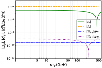
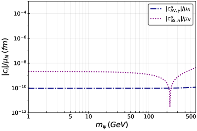
(a) Dirac DM (left) and Majorana DM (right) with a vector-like fermion $F$ of mass $m_{F}=600$ GeV and a scalar $S$ of mass $m_{S}=500$ GeV. The Yukawa couplings are fixed to $y_{V}=1$ and $y_{A}=1.3\,e^{i\,1.4}$.

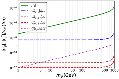
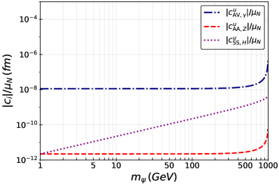
(b) Dirac DM (left) and Majorana DM (right) with left-handed SM leptons in the loop and a scalar $S$ of mass $m_{S}=1000$ GeV. All Yukawa couplings are fixed to $y_{2}=1$.

Figure 2: Wilson coefficients at the quark level (with up-type quarks) versus the DM mass $m_{\psi}$. The Higgs portal coupling is $\lambda_{HS}=3$. The vector and scalar coefficients which originate from the photon, $Z$ and Higgs penguin diagrams, respectively, have been rescaled by the nuclear magneton $\mu_{N}=e/(2m_{p})$. The photon penguin contribution $c^{u}_{{\rm VV},\gamma}$ depends on the transferred momentum $q$ for light SM leptons: We choose a recoil energy $E_{R}=8.59$ keV for ${}^{132}_{54}\mathrm{Xe}$ which results in $|\vec{q}|^{2}=2.11\times 10^{-3}\,\mathrm{GeV}^{2}$.

5.2 Wilson coefficients at the nucleon level

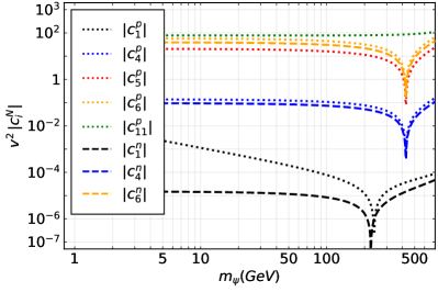
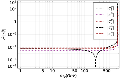
(a) Dirac DM (left) and Majorana DM (right) with a vector-like fermion $F$ of mass $m_{F}=600$ GeV and a scalar $S$ of mass $m_{S}=500$ GeV. The Yukawa couplings are fixed to $y_{V}=1$ and $y_{A}=1.3\,e^{i\,1.4}$.

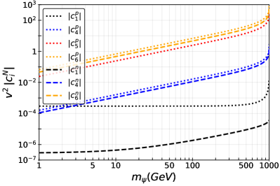
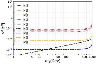
(b) Dirac DM (left) and Majorana DM (right) with left-handed SM leptons in the loop and a scalar $S$ of mass $m_{S}=1000$ GeV. All Yukawa couplings are fixed to $y_{2}=1$.

Figure 3: Non-relativistic nucleon level Wilson coefficients evaluated for ${}^{132}_{54}\mathrm{Xe}$ at $E_{R}=8.59$ keV (and thus $|\vec{q}|^{2}=2.11\times 10^{-3}\,\mathrm{GeV}$) versus the DM mass $m_{\psi}$. The Higgs portal coupling is $\lambda_{HS}=3$. All Wilson coefficients are displayed in dimensionless units by rescaling with the square of the electroweak VEV $v=246.2$ GeV.

The previous Wilson coefficients at the quark level can interfere and generate non-trivial effective operators at the nucleon level, see Sec. 3.2. We plot in Fig. 3 the NR Wilson coefficients with protons (neutrons) in dotted (dashed) lines ($N=n,\,p$ for neutrons and protons). All Wilson coefficients are displayed in dimensionless units, by rescaling them with the square of the electroweak VEV, $v=246.2$ GeV. As for Fig. 2, the upper panel is for vector-like fermions and the lower panel for SM left-handed lepton doublets. The plots on the left correspond to Dirac DM, while the plots on the right are for Majorana DM.

For a vector-like fermion $F$ (upper panels of Fig. 3), we fix $m_{F}=600$ GeV, $m_{S}=500$ GeV, $y_{V}=1$ and $y_{A}=1.3\,e^{1.4\,i}$. For Dirac DM (left plot), we show the coefficients short-range SI $c^{N}_{1}$ (black) and the SD scattering $c^{N}_{4}$ (blue), and the long-range contributions $c^{N}_{5}$ (red), $c^{N}_{6}$ (orange) and $c^{N}_{11}$ (green). Notice that both $c^{N}_{5}$ and $c^{N}_{11}$ are generated by the electric and magnetic DM dipole moments proportionally to the nucleon charge and they are therefore absent for neutrons. The long-range Wilson coefficients $c^{N}_{5}$, $c^{N}_{6}$ and $c^{N}_{11}$ dominate. The SD coefficients $c^{N}_{4}$ are more than two orders of magnitude smaller and very similar for protons and neutrons, although slightly larger for the former. The SI coefficients $c^{N}_{1}$ are the smallest ones, and $c^{p}_{1}$ decreases with the DM mass up to $m_{\psi}\simeq 500$ GeV. The difference in behavior of $c^{p}_{1}$ and $c^{n}_{1}$ stems mainly from the non-zero contribution of $\mu_{\psi}$ to the former ($c^{p}_{1}\propto\mu_{\psi}/m_{\psi}$). In this example the Wilson coefficients $c^{N}_{1}$ change sign at about $m_{\psi}\simeq 225$ GeV and $c^{N}_{4,5,6}$ at $m_{\psi}\simeq 425$ GeV. For Majorana DM with vector-like fermions (top right) the $c^{N}_{1}$ contributions generated by the Higgs penguin diagram (black) are very similar for protons and neutrons (they are superimposed in the plot). The anapole moment generates $c^{p}_{8}$ (solid purple), $c^{p}_{9}$ (solid magenta) and $c^{n}_{9}$ (dashed magenta) which are very similar, specially $c^{p}_{8}$, to the $c^{N}_{1}$ contributions (black). All the Wilson coefficients are in the range $10^{-5}-10^{-4}$, except in the region of DM mass when a Wilson coefficient changes sign at $m_{\psi}\simeq 225$ GeV.

For Dirac DM with SM leptons (bottom left) the phenomenology is very rich. The long-range Wilson coefficients $c^{p}_{5}$ (dotted red), $c^{p}_{6}$ (dotted orange) and $c^{n}_{6}$ (dashed orange) dominate ($c^{n}_{5}=0$, as it is proportional to the electric charge of the nucleon). They increase with the DM mass as they are generated dominantly by $\mu_{\psi}$, i.e., chirality needs to be violated. Similarly $c^{N}_{4}$ (blue) with $p$ (dotted) and $n$ (dashed) have a dominant contribution from $\mu_{\psi}$ and therefore increase with $m_{\psi}$. Regarding $c^{n}_{1}$ (dashed black), the increase of its slope reflects the fact that the short-range Higgs contribution (which grows with $m_{\psi}$) increasingly becomes more and more comparable to the photon short-range coefficient, but in any case $c^{n}_{1}$ remains very suppressed. $c^{p}_{1}$ is dominated by the photon penguin, and both the short-range contribution parameterized by $c_{VV,\gamma}^{q}$ and the long-range contribution from the magnetic moment $\mu_{\psi}/m_{\psi}$ are important. Due the dependence of the quark-level Wilson coefficients on the DM mass, the NR Wilson coefficient $c_{1}^{p}$ is basically constant with respect to it. For Majorana DM with SM leptons (bottom right) the Wilson coefficients $c^{p}_{8}$ (solid purple), $c^{p}_{9}$ (solid magenta) and $c^{n}_{9}$ (dashed magenta), which are generated by the anapole operator, dominate. $c^{N}_{6}$ ($c^{p}_{6}$ and $c^{n}_{6}$ are superimposed in the plot) do not increase with the DM mass, unlike in the Dirac case, because here they come from $c^{N}_{\rm AA}$ and not from $\mu_{\psi}$; $c^{N}_{1}$, generated by the Higgs penguin diagram, increases with $m_{\psi}$ and is very similar for $n$ and $p$ ($c^{n}_{1}$ and $c^{p}_{1}$ are superimposed in the plot). Finally, $c^{N}_{4}$, generated by the $Z$ penguin, are similar for both $n$ and $p$ (superimposed in the plot) and very suppressed, as expected.

5.3 Direct detection event rates

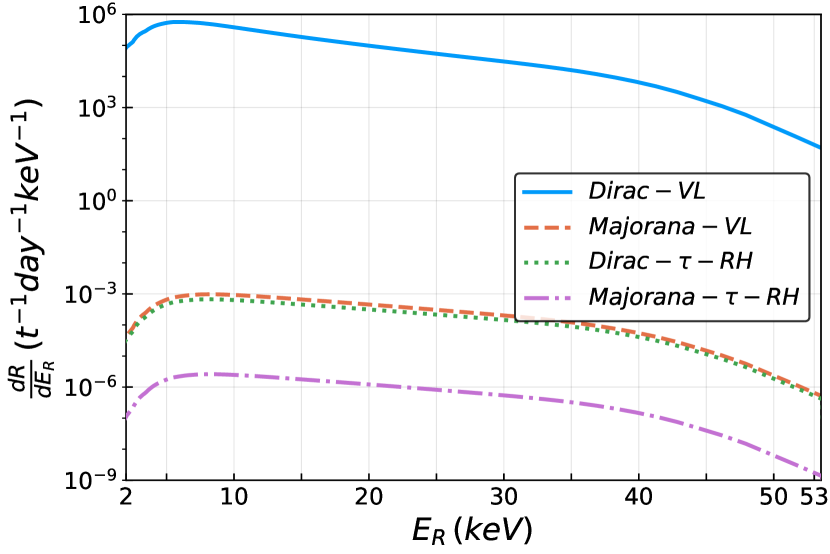
(a) Dirac vs. Majorana DM for a vector-like fermion and a right-handed $\tau$ lepton in the loop.

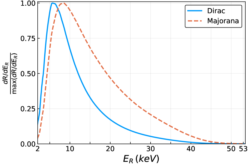
(b) Normalized spectrum for Dirac and Majorana DM with a vector-like fermion in the loop.

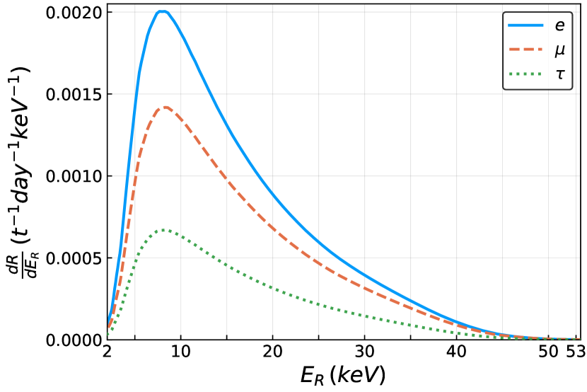
(c) Dirac DM with coupling to a right-handed lepton. A pure coupling to a left-handed lepton leads to the same result.

Figure 4: Differential event rates for different combinations of DM candidates and fermions in the loop. The DM mass is $m_{\psi}=90$ GeV and the Higgs portal coupling is $\lambda_{HS}=3$. In the case of a vector-like fermion $F$ and a scalar $S$ in the loop we fix $m_{F}=600$ GeV, $m_{S}=500$ GeV, $y_{V}=1$ and $y_{A}=1.3\,e^{i\,1.4}$. In the case of a right-handed $\tau$ lepton we fix $m_{S}=1000$ GeV and $y_{1}=1$.

The different Wilson coefficients are expected to generate different features in the DD differential spectrum. In the upper-left panel of Fig. 4 we plot the DD differential event rates in xenon versus the recoil energy $E_{R}$ for Dirac DM with a vector-like fermion $F$ (solid blue) and with a right-handed tau (dotted green), and for Majorana DM with a vector-like fermion (dashed red) and with a right-handed tau lepton (dot-dashed purple). For details on the astrophysical assumptions used in the numerical analysis see Ref. [63]. The rate for Dirac DM with a vector-like fermion is roughly $9$ orders of magnitude larger than that with a SM lepton (a tau lepton in this case), because in the latter case there is no contribution from the electric dipole moment $d_{\psi}$ and the magnetic dipole moment $\mu_{\psi}$ is suppressed by the DM mass $m_{\psi}$. The smallest rate occurs for Majorana DM with a right-handed tau in the loop. The relative size of the spectra is obvious from the relative size of the NR Wilson coefficients discussed in the previous section.

In the upper-right panel we show the spectrum normalized to the maximum value ($5.7\times 10^{5}\,[9.7\times 10^{-4}]\,{\rm t^{-1}\,day^{-1}\,{\rm keV}^{-1}}$ for Dirac [Majorana] DM) for the case with vector-like fermions in the loop, for Dirac DM (solid blue) and Majorana DM (dashed red). The spectral shapes are quite different, which is mainly due to the fact that there are no dipole moments for Majorana DM.

In the bottom panel of Fig. 4 we plot the DD differential rates for Dirac DM with coupling to a right-handed electron (solid blue), muon (dashed red) and tau (dotted green). The spectra are the largest for the electron (the lightest lepton), with maxima at roughly the same recoil energy. The maxima go approximately in the ratios $\sim(4:2:1)$ for $e,\mu,\tau$. This is due to the dependence on the short-range contribution of the photon penguin, $c^{q}_{VV,\gamma}$, via the NR Wilson coefficient $c_{1}^{p}$. The spectra are dominated by the photon short-range contribution $c^{q}_{VV,\gamma}$ for this choice of parameters.

5.4 Direct detection limits

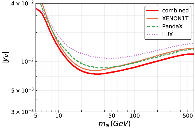
(a) Dirac DM for different xenon experiments.

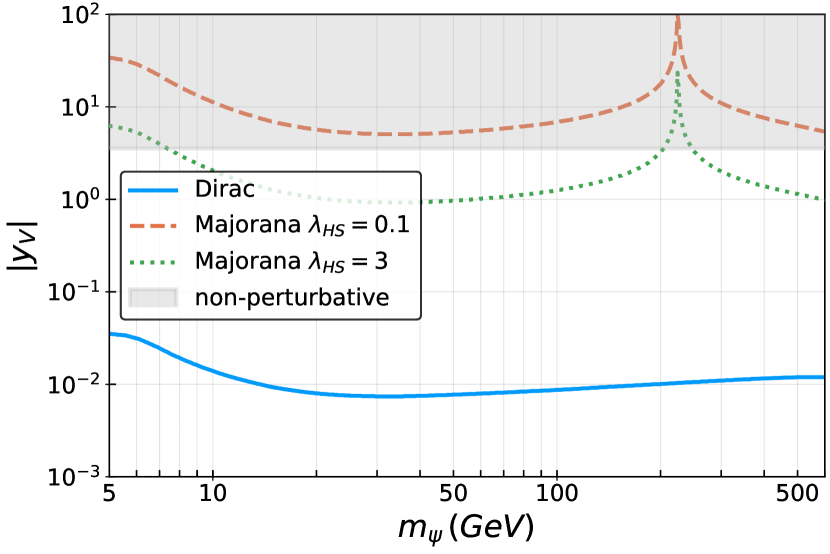
(b) Different DM candidates and couplings.

Figure 5: DM direct detection $90\%$ C.L. limits with a vector-like fermion in the loop. We fix $m_{S}=500$ GeV, $m_{F}=600$ GeV, the ratio of Yukawa couplings $|y_{A}|/|y_{V}|=1.3$ and the phases of the Yukawa couplings are $\phi_{V}=0$ and $\phi_{A}=1.4$. Unless specified the Higgs portal coupling is $\lambda_{HS}=0.1$. We highlight in gray the region where the Yukawa coupling is non-perturbative, $|y_{V}|>\sqrt{4\pi}$.

Next we study the upper limits that current DD experiments can impose on the scenarios discussed so far. In order to illustrate current direct detection limits, we consider different scenarios of TeV-scale dark sectors. We also discuss how the limits vary with the masses of the particles in the loop. We show the $90\%$ C.L. upper limits from current DD experiments that have xenon as a target, which provide the most stringent limits for SI interactions for our range of DM masses. We show $m_{\psi}\gtrsim 5$ GeV, as very light DM does not produce recoils at energies above the threshold of the DD experiments. The limits are subject to large uncertainties from nuclear physics and astrophysics as well as from experimental uncertainties. In the following we do not show limits from Higgs and $Z$ boson invisible decay widths into DM, as those are weaker than the ones coming from DD in our scenarios. In Sec. 6.2 we discuss some examples where these limits can be relevant, and complementary to DD, specially for light DM masses, and in App. C we provide the relevant expressions for the Higgs and $Z$ boson invisible decay rates.

In the left panel of Fig. 5 we plot the upper limits for Dirac DM in the plane $|y_{V}|$ versus $m_{\psi}$ for XENON1T (solid brown), PandaX (dashed green) and LUX (dotted purple), together with their combined limit (thicker solid red line). We have fixed $m_{S}=500$ GeV, $m_{F}=600$ GeV, $\lambda_{HS}=0.1$, the ratio of Yukawa couplings $|y_{A}|/|y_{V}|=1.3$ and the phases of the Yukawa couplings $\phi_{V}=0$ and $\phi_{A}=1.4$. As expected the bounds are weakened at very large and very small DM masses. At large DM masses the limits appear to approach a constant value, instead of decreasing as $1/m_{\psi}$ as expected from the DM number density. This is due to the non-trivial dependence of the Wilson coefficients on $m_{\psi}$. In particular the Wilson coefficients generally increase for $m_{\psi}\rightarrow m_{F}+m_{S}$. The $|y_{V}|$ limits are of the order of $\sim 10^{-2}$ for a large range of DM masses between 10 GeV and 500 GeV. This is a clear example of the superb sensitivity achieved by DD experiments, which are able to probe such small Yukawa couplings for loop-induced scenarios of Dirac DM.

In the right panel of Fig. 5 we show the limits for Majorana DM with $\lambda_{HS}=0.1$ (dashed red) and $\lambda_{HS}=3$ (dotted green), together with those for Dirac DM (solid blue). The current limits for Majorana DM are very weak, close to the naive perturbativity limit. Notice that the Higgs interactions are non-negligible: changing $\lambda_{HS}=0.1$ to $\lambda_{HS}=3$ the upper bound on the Yukawa couplings improves by a factor of $\sim 6$ (at the level of the rate, the scalar quartic coupling enters quadratically, while the Yukawa couplings enter to the fourth power). The difference with respect to the strong limits for Dirac DM stems, of course, from the absence of dipole moments for Majorana DM. In the gray shaded region, the Yukawa coupling is non-perturbative, $|y_{V}|>\sqrt{4\pi}$, and therefore the one-loop computation cannot be trusted.

5.5 Interplay with lepton flavor violation and relic abundance

When there are SM charged leptons running in the loop, there may also be limits from LFV processes. We provide the relevant expressions for $\ell_{\alpha}\rightarrow\ell_{\beta}\gamma$, $\mu-e$ conversion and $\ell_{\alpha}\rightarrow\ell_{\beta}\ell_{\gamma}\ell_{\delta}$ in App. D. It is therefore interesting to study the interplay between both types of signals. Although one may naively expect that LFV limits are stronger (because an accidental symmetry of the SM is violated), we see in the following that this is not the case in all scenarios.

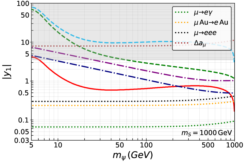
(a) Equal leptons couplings. $m_{S}=1000$ GeV.

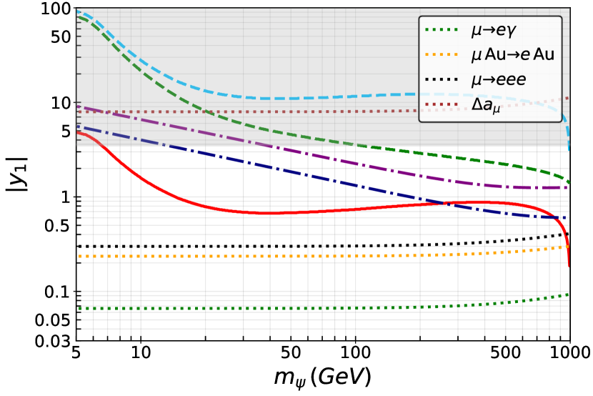
(b) No coupling to $\tau$ leptons. $m_{S}=1000$ GeV.

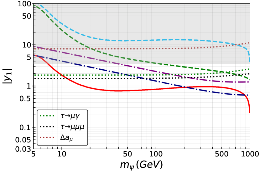
(c) No coupling to electrons. $m_{S}=1000$ GeV.

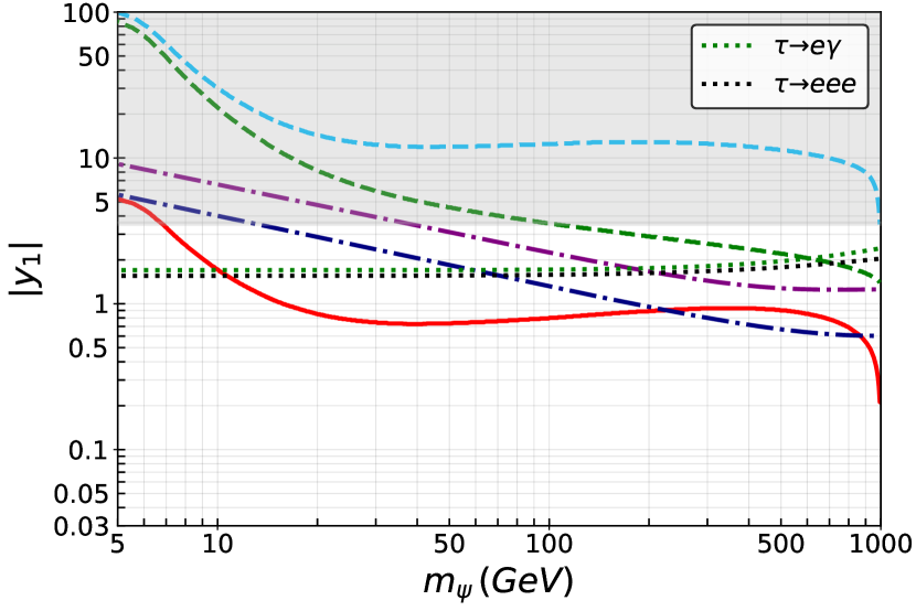
(d) No coupling to muons. $m_{S}=1000$ GeV.

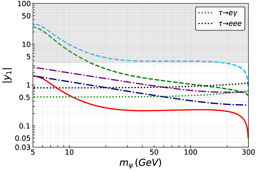
(e) No coupling to muons. $m_{S}=300$ GeV.

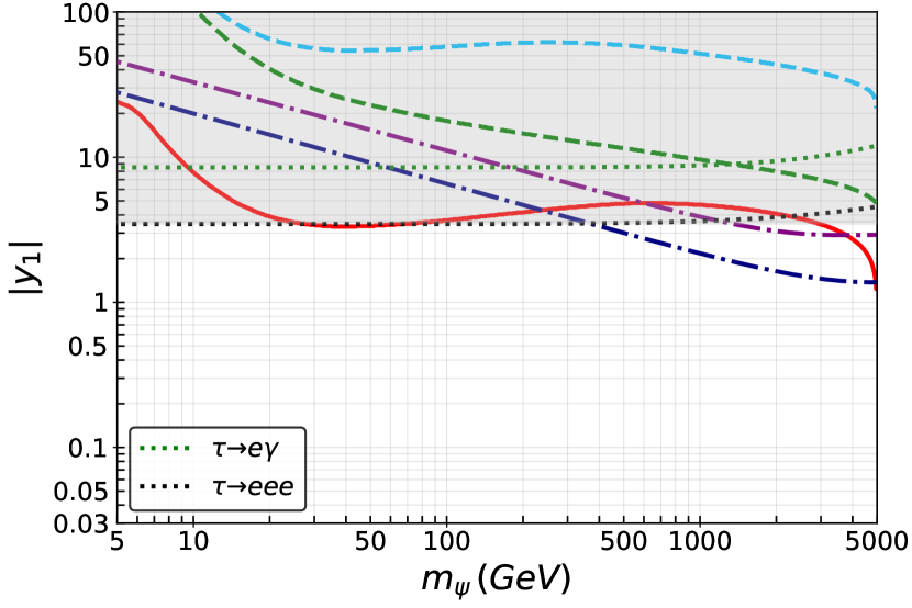
(f) No coupling to muons. $m_{S}=5000$ GeV.

Figure 6: Combined direct detection $90\%$ C.L. limits for Dirac dark matter (solid red), and Majorana dark matter with $\lambda_{HS}=0.1$ (dashed light blue) and $\lambda_{HS}=3$ (dashed green), with right-handed charged leptons in the loop. Contours of the correct relic abundance set by $\psi\psi\rightarrow\ell_{\alpha}\ell_{\beta}$ annihilations mediated by the scalar $S$ are shown as dot-dashed navy blue (purple) line for Dirac (Majorana) dark matter. The dotted lines indicate constraints from the relevant LFV processes. In the gray shaded region the Yukawa coupling is non-perturbative, $|y_{1}|>\sqrt{4\pi}$.

In Fig. 6, top-left panel, we plot the DD upper limits in the plane $|y_{1}|$ versus $m_{\psi}$, assuming equal couplings to all leptons, i.e., $y^{e}_{1}=y^{\mu}_{1}=y^{\tau}_{1}=y_{1}$ (we denote this the “symmetric” case). In Fig. 6 top-right, middle-left and middle-right panels we show the cases of no couplings to taus, electrons and muons, respectively. Left-handed and right-handed leptons in the loop lead to the same result. We show the cases of Dirac DM (solid red), and Majorana DM with $\lambda_{HS}=0.1$ (dashed light blue) and $\lambda_{HS}=3$ (dashed green). We have fixed $m_{S}=1000$ GeV for the four upper plots. The most relevant $90\%$ C.L. LFV limits are shown using dotted lines: $\mu\rightarrow e\gamma$ (green), $\mu-e$ conversion (orange), $\mu\rightarrow 3e$ (black) and $\Delta a_{\mu}$ (brown). Notice that LFV limits do not depend on whether the DM is a Dirac or Majorana fermion. Also, we emphasize once more that DD limits are subject to large astrophysical and nuclear uncertainties, which are absent in the case of LFV experiments.

In addition we plot the contour of the DM relic abundance, set by t-channel DM annihilations $\psi\psi\rightarrow\ell_{\alpha}\ell_{\beta}$ mediated by the scalar $S$, with a dot-dashed navy blue (purple) line for Dirac (Majorana) DM, whose leading contribution is from s-wave (p-wave) scattering. We use the instantaneous freeze-out approximation which is sufficient for our purposes (see Sec. 6.3.1 and App. E for more details and the relevant expressions). Above the $\Omega h^{2}$ contour the DM would be under abundant and requires an additional component of DM to account for the observed relic abundance. Below the $\Omega h^{2}$ contour DM is over abundant if its abundance is solely set by freeze-out, and thus there has to be a mechanism to further deplete its density. It could be reduced via co-annihilation and resonant effects [20], multi-body scatterings [64, 65, 66, 67, 68], or a non-trivial thermal evolution in the early universe [69]. In case $\psi$ does not account for all of the DM abundance the DD limits have to be rescaled appropriately. Assuming thermal freeze-out reproducing the correct relic abundance imposes a lower bound on the DM mass. In the case of equal couplings to all leptons with $m_{S}=1000$ GeV, $m_{\psi}\gtrsim 10\,(25)$ GeV for Dirac (Majorana) DM. When one final channel is closed, the lower limits increase by roughly $5\,(15)$ GeV for Dirac (Majorana) DM. For light scalar mass (see bottom-left panel of Fig. 6), all Yukawa couplings are perturbative. However, for heavy $m_{S}$, bottom-right panel, the Yukawa couplings are perturbative only for very heavy masses, above $0.4\,(1)$ TeV, as in this case the t-channel interaction is significantly suppressed by the mass of the mediator.

The main changes in the case of no couplings to taus, electrons and muons (top-right, middle-left and middle-right panels in Fig. 6) are in the LFV limits, as depending on the flavor structure, different processes are possible. In these panels the relic abundance contours are almost identical, as the SM leptons are always much lighter than the DM (and therefore phase space plays no significant role). Of course, the contours are at somewhat larger Yukawa couplings than for the “symmetric” scenario, as in the latter there were more available annihilation channels. The DD limits are also slightly modified due to the different masses of SM leptons in the loop (see also the lower panel of Fig. 4). When there are no couplings to taus (top-right panel), the LFV limits are almost identical to the “symmetric” scenario, because they are driven by the first family. However, for no couplings to electrons or muons (middle panels), DD limits are more stringent than LFV limits for Dirac DM with a mass above a certain value. This is quite remarkable: DD experiments are able to better constrain scenarios where an accidental symmetry of the SM is violated than experiments directly searching for it. Interestingly, limits on $|y_{1}|$ from trilepton $\tau$ decays ($\tau\rightarrow 3\ell$) dominate over radiative $\tau$ decays ($\tau\to\ell\gamma$) in contrast to the limits from muon decays. As the limits from $\tau$ decays are generally weaker and thus the corresponding Yukawa couplings larger, box-diagram contributions to trilepton decays may give a sizable contribution and thus break the dipole dominance.

A few interesting remarks can be drawn from these plots. First, note that the DD limits with SM leptons in the loop, even for Dirac DM, are much weaker than in the scenario with vector-like fermions in the loop, as also demonstrated in the top-left panel of Fig. 4. Second, clearly the LFV limits are the strongest ones, with $\mu\rightarrow e\gamma$ the most stringent among them. Its limit on the Yukawa coupling $|y_{1}|$ is a factor of a few stronger than the one of DD for Dirac DM. Again, the DD limits become very strong close to $m_{\psi}\rightarrow m_{S}+m_{F}$ as in the case with vector-like fermions. Third, for scalar masses at the TeV scale, the DD limit already excludes the production via thermal freeze-out for Majorana DM, and also for Dirac DM in the mass range $5~{}\text{GeV}\lesssim m_{\psi}\lesssim 200$ GeV. Finally, the muon AMM constraint is always very weak, being the limit above the perturbativity bound.

In Fig. 6, bottom panels, we show two examples of a scalar $S$ in the loop with a different mass: $m_{S}=300$ GeV (left plot) and $m_{S}=5000$ GeV (right plot). All limits are generically stronger for $m_{S}=300$ GeV and weaker for $m_{S}=5000$ GeV compared to $m_{S}=1000$ GeV. In particular, the relative contribution of the box diagrams and the dipole moment for the trilepton $\tau$ decay changes: for $m_{S}=300$ GeV $\tau\rightarrow e\gamma$ sets a stronger limit than $\tau\to 3e$. Similarly the Yukawa coupling required to explain the observed relic abundance also has to be larger for heavier scalar masses, as already discussed. Indeed, for $m_{S}=5000$ GeV almost all the limits on the Yukawa couplings are in the non-perturbative region.

In summary, strong limits can be set for Dirac DM with vector-like fermions in the loop. For Dirac DM with SM leptons in the loop LFV limits or DD limits may set the strongest bounds depending on the flavor structure and the DM mass. Therefore, the two limits are complementary: LFV limits are more important for DM coupling to both muons and electrons, whereas DD limits dominate if there are no LFV processes of type $\mu\to eX$, $X$ being anything, and the DM mass is not too small ($m_{\psi}\gtrsim 5$ GeV). For Majorana DM, LFV limits, if present, are generally more stringent than constraints from DD. Future DD experiments and LFV limits on $\tau$ decays are expected to improve by 1-2 orders of magnitude and hence the situation is not expected to change dramatically. If $\mu-e$ conversion in nuclei and/or $\mu\rightarrow 3e$ expected sensitivities (by several orders of magnitude) are achieved, LFV limits will continue to dominate and even increase their difference with respect to DD.

6 Other phenomenological aspects

6.1 LHC searches

Generally colliders may only set competitive limits via missing energy searches for light DM and SD interactions. In the scenarios discussed here, naively the production of DM particles at the LHC occurs at one-loop level via the penguin diagrams in Fig. 1 and is therefore suppressed. For example, Ref. [25] showed that there are only very weak collider limits on a model with a magnetic moment interaction. Thus it is more promising to search for the mediators $S$ and $F$ at colliders via $q\bar{q}\rightarrow F\bar{F},SS^{*}$ mediated by the photon, the $Z$ boson and/or the Higgs. If the new fermion and scalar have electric charge, the production is dominated by the Drell-Yan process. Higgs-mediated production of exotic particles has been discussed in e.g. Ref. [70]. As we are assuming that the new particles are not colored, only modest lower limits (below $1$ TeV) are expected, unless very large SM quantum numbers (for instance electric charges) are invoked. The dark sector particles may decay invisibly into DM and a lighter dark sector state. The phenomenology of these decays are however model-dependent, see discussion in Sec. 2. Another interesting option would be to search for DM in models with electrons/muons running in the loop at future lepton colliders. The main production process is via $t$-channel exchange of the scalar, $\ell^{+}\ell^{-}\rightarrow\psi\bar{\psi}$ with $\ell=e,\mu$.

6.2 $Z$ and Higgs boson invisible decays

If the DM $\psi$ is sufficiently light [$m_{\psi}<m_{H}/2\,\left(m_{Z}/2\right)$] there is an additional contribution to the invisible width of the Higgs ($Z$) boson. In App. C we present the relevant expressions for these processes. We find that there are no limits from $Z$ or Higgs boson decays into DM for the parameter values used in Figs. 5 and 6. However, there may be limits for small scalar/fermion/DM masses and large Yukawa couplings. To illustrate this point we plot in Fig. 7 the branching ratios ${\rm Br}(Z\rightarrow\psi\psi)$ (left plot) and ${\rm Br}(h\rightarrow\psi\psi)$ (right plot), for Dirac (Majorana) DM with solid (dashed) lines. For the SM widths we use $\Gamma_{h,{\rm SM}}=4.1$ MeV and $\Gamma_{Z,{\rm SM}}=2.495$ GeV, such that the Higgs branching ratio reads ${\rm Br}(h\rightarrow\psi\psi)=\Gamma_{h\rightarrow\psi\psi}/(\Gamma_{h,SM}+\Gamma_{h\rightarrow\psi\psi})$ and similarly for the $Z$ boson. We show the cases of different particles running in the loop with solid lines: in black the case of vector-like fermions with $Q_{F}=Y_{F}=-1$ and in red (blue) the case of a tau-lepton doublet (singlet). For Higgs decays the tau-lepton doublet and the singlet generate the same branching ratio, shown in blue. The experimental upper limits on invisible non-SM decays are shown as horizontal gray lines: solid for the $Z$ boson from LEP (the total invisible width of the $Z$ including neutrinos is $\Gamma_{\rm Z\rightarrow{\rm inv}}=499.1\pm 1.5$ MeV [71]), and dot-dashed (dashed) for the Higgs from CMS [72] (ATLAS [73]), which reads ${\rm Br}(h\rightarrow{\rm inv})<0.24\,(0.28)$ at $95\%$ CL. We used $m_{S}=120$ GeV and $m_{F}=150$ GeV and a Higgs portal coupling $\lambda_{HS}=0.2$. For vector-like fermions in the loop we used $y_{V}=4\,e^{i\pi/3}$ and $y_{A}=3\,e^{i\pi/4}$, while for SM tau-lepton doublets [singlets] we fixed $y_{V}=[-]\,y_{A}=4\,e^{i\pi/3}$.

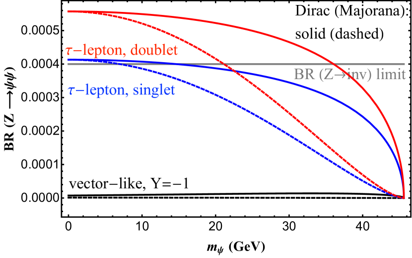
(a) Branching ratio of the $Z$ boson into DM.

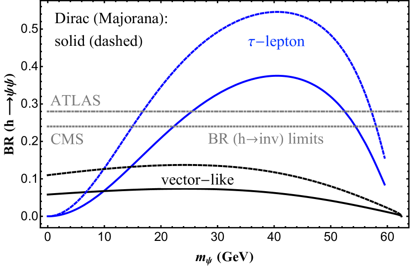
(b) Branching ratio of the Higgs boson into DM.

Figure 7: Branching ratios of the $Z$ and the Higgs bosons decaying invisibly into DM (Dirac in solid, Majorana in dashed). We show in black the case of vector-like fermions in the loop, in red the case of a tau-lepton doublet and in blue the case of tau-lepton singlet. The experimental upper limits on non-SM invisible decays are displayed as horizontal gray lines. See the text for details.

In Fig. 7 one can observe that the limits for Dirac DM are stronger than those for Majorana DM in the case of $Z$ boson decays, independently of the particles in the loop, while the situation is the opposite in the case of Higgs decays. Also, invisible $Z$ boson decays constrain light DM which couples to SM leptons (the tau in this case). For Dirac DM the limits exclude DM masses below $14\,(36)$ GeV in the case of couplings to tau singlets (doublets). The width is dominated by $c_{V}$ and $c_{A}$, while $d_{A}\simeq 0$ and $d_{V}$ is suppressed by $m_{\psi}$. For vector-like fermions the width is dominated by $d_{V}$ and $d_{A}$ with $d_{V}>d_{A}$, and there are no relevant limits. For Majorana DM the limits are weaker than for Dirac DM, demanding $m_{\psi}\gtrsim 6\,(21)$ GeV in the case of couplings to tau singlets (doublets), with no limits in the case of couplings to vector-like leptons.

As in the case of the $Z$ boson, the decays of the Higgs boson do not pose limits on the scenario with vector-like fermions in the loop. For the tau-lepton $b_{A}=0$ and the dominant contribution to $b_{V}$ is proportional to $m_{\psi}$, as $m_{F}\ll m_{\psi}$. The branching ratio increases with the DM mass for low DM masses, while at some DM mass value ($\simeq 40$ GeV in the plot) the phase space suppression dominates and the branching ratio decreases again. Therefore there is a constraint on an intermediate DM mass range of $[25,\,53]$ GeV ($[22,\,55]$ GeV) by ATLAS (CMS) for Dirac DM and $[16,\,57]$ GeV ($[14,\,58]$ GeV) by ATLAS (CMS) for Majorana DM.

To summarize, while for vector-like fermions there are no limits, for SM particles in the loop there may be interesting constraints in the absence of LFV. Indeed, there is a well-known complementarity between invisible decays and DD. The experimental energy threshold of DD experiments limits their ability to impose limits for arbitrarily low DM masses and thus invisible decays may set competitive limits for low DM masses.

6.3 Relic abundance

The production of the correct relic DM density in the early universe is generally model-dependent. Although it is not the main focus of this work, we briefly outline different avenues to obtain the correct relic density. See e.g. Ref. [74] for a connection of DD with thermal freeze-out.

6.3.1 Thermal freeze-out

If $m_{\psi}>m_{S},m_{F}$ (but of course $m_{\psi}<m_{S}+m_{F}$), the relic abundance can be set via the t-channel interactions $\psi\bar{\psi}\rightarrow SS^{*}$ or $\psi\bar{\psi}\rightarrow F\bar{F}$. Subsequently, $S$ and $F$ can decay to SM particles, in some cases at loop level or via non-renormalizable operators. In particular if $F$ is a SM lepton $\ell_{\alpha}$, DM annihilations to SM leptons $\psi\bar{\psi}\rightarrow\ell_{\alpha}\bar{\ell}_{\beta}$ may set the relic abundance. For Dirac DM the cross section is not velocity suppressed and thus the leading (s-wave) part of the thermally averaged annihilation cross section is given by

$$\left.\left\langle\sigma v\right\rangle\right|_{\text{D}}=\frac{m_{\psi}^{2}}{32\pi(m_{\psi}^{2}+m_{S}^{2})^{2}}\,\sum_{\alpha,\beta}|y_{i,\beta}y_{i,\alpha}^{*}|^{2}\,,$$ (45)

where we have summed over all possible final state leptons (neutrinos and charged leptons) in the limit of vanishing lepton masses. Here $i=1\,(2)$ for couplings to LH (RH) leptons, see Eq. (1). For Majorana DM the annihilation cross section is velocity suppressed and the leading contribution is due to p-wave scattering

$$\left.\left\langle\sigma v\right\rangle\right|_{\text{M}}=\frac{m_{\psi}^{2}\left(m_{S}^{4}+m_{\psi}^{4}\right)}{8\pi x\left(m_{S}^{2}+m_{\psi}^{2}\right)^{4}}\,\sum_{\alpha,\beta}|y_{i,\beta}y_{i,\alpha}^{*}|^{2}\,,\\$$ (46)

where $x=m_{\psi}/T$.

As discussed in App. E, for DM masses in the range $10\,\text{GeV}\lesssim m_{\psi}\lesssim 10^{4}\,\text{GeV}$ we obtain the correct relic abundance for cross sections $\left.\left\langle\sigma v\right\rangle\right|_{\text{D}}\simeq[2,3]\cdot 10^{-26}\,{\rm cm^{3}\,s^{-1}}$ for Dirac DM and $\left.\left\langle\sigma v\right\rangle\right|_{\text{M}}\simeq[0.5,1]\cdot 10^{-23}\,{\rm cm^{3}\,s^{-1}}$ for Majorana DM. Equating these values to Eq. (45) and Eq. (46), respectively, we plot in Fig. 6 the relic abundance contours in the $|y_{1}|-m_{\psi}$ plane.

If $\psi$ is the lightest particle in the dark sector (i.e., $m_{\psi}<m_{S},m_{F}$), DM may annihilate at one-loop order into quarks via the penguin diagrams in Fig. 1. However this is very suppressed and results in an over abundance of DM and requires another mechanism: (i) In a larger dark sector DM may annihilate into other lighter dark particles, $\psi\psi\rightarrow XX$ which subsequently decay to SM particles. These new light particles may lead to large DM self-interactions, see for instance Ref. [78]. (ii) Co-annihilation and resonant effects [20] may increase the effective thermal annihilation cross section. For example processes like $\psi\bar{F}\rightarrow S^{*}\rightarrow HH$ with $(m_{F}-m_{\psi})/m_{\psi}\simeq 1/20$ could be induced by a coupling of $S$ to the SM Higgs. Similarly there may be coannihilations with $S$. If $S$ has gauge interactions the dominant channel may be $SS\to\text{SM\,SM}$ (see for instance Ref. [79]) if $(m_{F}-m_{\psi})/m_{\psi}\simeq 1/20$ and $\psi$ and $S$ are in thermal equilibrium. (iii) Multi-body scatterings may also increase the effective thermal annihilation cross section [64, 65, 66, 67, 68]. (iv) A non-trivial thermal evolution in the early universe may depopulate an initially over abundant DM relic density [69].

6.3.2 Non-thermal production

The DM abundance may also be produced non-thermally. If DM is only very weakly coupled to the SM thermal bath and it has not been produced during reheating, DM may be slowly produced via the freeze-in mechanism [39, 40]. Ref. [30] discussed the phenomenology of the freeze-in mechanism in the scotogenic model [9] with fermionic DM, one of the examples where DM-nucleus scattering occurs at one-loop level.

7 Conclusions

Direct detection of DM may not have been observed yet because it is absent at tree level, occurring only at the loop level. In this work we have studied the case of a fermionic singlet DM $\psi$, which is a simple scenario where DD is naturally induced at one-loop order. The type of scenario considered appears in supersymmetric extensions where the neutralino is pure bino [15] (notice that in this case its mass is typically very heavy, larger than 2 TeV), and also in connection to neutrino masses, in particular in the seesaw model [13] and in some radiative neutrino mass models [9, 8, 12, 80]. We have considered a simplified scenario with a dark sector made of a vector-like (or a SM) fermion and a (complex) scalar. We presented general analytical expressions for the different contributions as well as current limits on the dark sector parameters. We have outlined the possible UV completions of the corresponding penguin diagrams, also those involving SM fields, and we summarize the different possibilities in the following:

(i) If the fermion is a SM lepton and thus leptophilic, the DM interactions are generically flavored [5] and there is an interesting phenomenology. There may be new contributions to the anomalous magnetic moment, but the limit is very weak. If there are couplings to at least two different flavors, there are strong limits from LFV, especially for couplings to both electrons and muons. In this case the limits from LFV processes such as $\mu\to e\gamma$ and $\mu\to 3e$ are much stronger than DD. In the absence of one of these couplings DD limits are stronger above a certain DM mass given by the experimental energy thresholds of the DD experiments. In some cases the same particles entering in the DD loop may naturally violate lepton number (specially if the DM couples to the left-handed lepton doublets) and give rise to radiative neutrino mass models such as the scotogenic model with Majorana DM [9] or the generalized scotogenic model with Dirac DM [80].

(ii) If the dark fermion is a right-handed neutrino, it may be a Majorana fermion and an active Majorana neutrino mass term is generated via the seesaw mechanism [81]. As the particles in the loop are neutral, DD is generated via $Z$ and Higgs penguin diagrams [13], which are very suppressed. Although the DM may be assigned lepton flavor and lepton number, there are no strong limits from LFV or lepton number violation beyond those already present in seesaw scenarios. This scenario is normally referred to as the neutrino-portal to DM [13, 41, 42].

(iii) If the scalar is the SM Higgs, there is mixing between the DM and the neutral component of the fermion in the loop, which generates tree-level contributions mediated by the $Z$ boson and the Higgs. The $Z$-mediated tree-level DD is expected to dominate with respect to the dipole moment contributions arising at loop level. In fact, elastic $Z$-mediated contributions are already ruled-out by DD experiments.

While the correct relic abundance is easily achieved in models with DM couplings to SM leptons (or not too heavy right-handed neutrinos), it requires further model-building in the case of DM couplings to vector-like fermions. We have also found that the invisible loop-induced $Z$ and Higgs boson decays may sometimes impose restrictions in the case of light DM.

In this work we studied the prototypical case of fermion singlet DM with the simplest dark sector, where the loop suppression still allows reasonably large DM interactions. Hopefully a positive DD signal in the next years will serve as a motivation and guidance to continue exploring the WIMP DD theory space and its interplay with other beyond the Standard Model probes.

Appendix A Larger dark matter groups

In the main part of the text we restricted ourselves to a global U(1) symmetry for a Dirac DM and to a discrete $Z_{2}$ symmetry for a Majorana DM. Our results can be easily generalized if the DM forms a larger non-trivial representation of the dark symmetry group and there are multiple degenerate components of the DM multiplet. As the dark symmetry commutes with the SM gauge group it simply leads to an overall factor of

$$\sum_{\gamma}(C^{\gamma\dagger}C^{\gamma})_{\alpha^{\prime}\alpha}\equiv\sum_{\beta,\gamma}C^{\gamma*}_{\beta\alpha^{\prime}}C^{\gamma}_{\beta\alpha}$$ (47)

to the Wilson coefficients of a DM particle-nucleus scattering, $\psi_{\alpha}N\to\psi_{\alpha^{\prime}}N$, where the Clebsch-Gordan coefficients $C_{\beta\alpha}^{\gamma}$ are defined such that the scalar and the two fermions are invariant under the dark sector symmetry:

$$C_{\beta\alpha}^{\gamma}\bar{F}_{\beta}S_{\gamma}\left(y_{1}P_{L}+y_{2}P_{R}\right)\psi_{\alpha}\;.$$ (48)

Thus for a general DM candidate with $N$ components $\psi_{\alpha}$ the DD cross section is obtained by summing over the final states and averaging over the initial state and thus

$$\sigma\to\frac{\sigma}{N}\sum_{\gamma,\delta}\mathrm{Tr}\left(C^{\gamma\dagger}C^{\gamma}C^{\delta\dagger}C^{\delta}\right)\;.$$ (49)

Note that a larger dark sector symmetry may lead to multiple DM candidates, which requires to go beyond the discussed scenario, see for instance Ref. [83].

Appendix B Direct detection differential cross section and event rate

The differential cross section for fermionic DM may be written in terms of NR operators at the nucleon level [52]

$$\frac{d\sigma}{dE_{R}}=\frac{m_{A}}{2\pi v^{2}}\frac{4\pi}{2J_{A}+1}\sum_{\tau,\tau^{\prime}=\{0,1\}}\Big{[} R_{M}^{\tau\tau^{\prime}}W_{M}^{\tau\tau^{\prime}}(|\vec{q}|)+R_{\Sigma^{\prime\prime}}^{\tau\tau^{\prime}}W_{\Sigma^{\prime\prime}}^{\tau\tau^{\prime}}(|\vec{q}|)+R_{\Sigma^{\prime}}^{\tau\tau^{\prime}}W_{\Sigma^{\prime}}^{\tau\tau^{\prime}}(|\vec{q}|)$$ (50)

$$+\frac{|\vec{q}|^{2}}{m_{N}^{2}}\left(R_{\Delta}^{\tau\tau^{\prime}}W_{\Delta}^{\tau\tau^{\prime}}(|\vec{q}|)+R_{\Delta\Sigma^{\prime}}^{\tau\tau^{\prime}}W_{\Delta\Sigma^{\prime}}^{\tau\tau^{\prime}}(|\vec{q}|)\right)\Big{]}$$

with the nucleus mass $m_{A}$ and spin $J_{A}$. The coefficients $R_{X}$ are given in terms of the NR Wilson coefficients $c_{i}^{0,1}=(c_{i}^{p}\pm c_{i}^{n})/2$ and $W_{X}$ denote the nuclear response functions. The explicit forms of $R_{X}$ and $W_{X}$ are given in Ref. [50]. For $|\vec{q}|\to 0$, the long wavelength limit, $W_{M}(0)\propto A^{2}$ counts the number of nucleons in the nucleus, $W_{\Sigma^{\prime\prime}}$ and $W_{\Sigma^{\prime}}$ measure the nucleon spin content of the nucleus, $W_{\Delta}$ measures the nucleon angular momentum and $W_{\Delta\Sigma^{\prime}}$ the interference.

In the literature it is also common to show the differential cross section as the sum of different dipole and charge contributions. Neglecting the $Z$ contributions to SD interactions, which are suppressed with respect to the long-range interactions, and taking $d_{\psi}=0$, the differential cross section can be written as [84]:

$$\frac{\text{d}\sigma}{\text{d}E_{R}}=\, \frac{\alpha^{2}_{\text{em}}}{4\pi}\mu_{\psi}^{2}Z^{2}\left(\frac{1}{E_{R}}-\frac{m_{A}}{2\mu_{\psi\text{A}}^{2}v^{2}}\right)F^{2}_{\text{SI}}\left(E_{R}\right)$$ (51)

$$+\alpha^{2}_{\text{em}}\frac{\mu_{A}^{2}\mu^{2}_{\psi}m_{A}}{4\pi^{2}v^{2}}\,\frac{J_{A}+1}{3J_{A}}\,F^{2}_{\text{SD}}\left(E_{R}\right)$$

$$+\frac{m_{A}}{2\pi v^{2}}A^{2}_{\rm eff}F^{2}_{\text{SI}}\left(E_{R}\right)\,,$$

where $\mu_{\psi A}=m_{\psi}m_{A}/(m_{\psi}+m_{A})$ is the DM–nucleus reduced mass and $A_{\rm eff}$ encodes the DM-nucleus couplings (see e.g. Ref. [10]):

$$A_{\rm eff}=Z\left(c_{\text{SI}}^{{\rm p},Z}+c_{\text{SI}}^{{\rm p},\gamma}+c_{\text{SI}}^{{\rm p},H}-\frac{\alpha_{\text{em}}\mu_{\psi}}{2\pi m_{\psi}}\right)+(A-Z)\left(c_{\text{SI}}^{{\rm n},Z}+c_{\text{SI}}^{{\rm n},H}\right)\;.$$ (52)

The first line in Eq. (51) corresponds to the dipole-charge (D-C), the second line to the dipole-dipole (D-D) and the third line to the charge-charge (C-C) interaction. $F_{\text{SI}}\left(E_{R}\right)$ and $F_{\text{SD}}\left(E_{R}\right)$ are the nuclear form factors. $c_{\text{SI}}^{{\rm N}}$ with $N=n,p$ are the relativistic Wilson coefficients at the nucleon level for the operators

$$\mathcal{O}_{\rm SI}^{\rm N,V} =\bar{\psi}\gamma_{\mu}\psi\bar{N}\gamma^{\mu}N\,, \mathcal{O}_{\rm SI}^{\rm N,H} =\bar{\psi}\psi\bar{N}N\;.$$ (53)

The vector operator $\mathcal{O}_{\rm SI}^{\rm N,V}$ is induced by both interactions with a photon and a $Z$ boson.

Once the differential cross section is computed via Eq. (50), the differential event rate per unit detector mass (for a detector with just one type of nucleus $A$) is given by:

$$\frac{\mathrm{d}R}{\mathrm{d}E_{R}}=\frac{\rho_{\psi}}{m_{\psi}m_{A}}\int_{v_{\rm min}(E_{\rm R})}\frac{\mathrm{d}\sigma}{\mathrm{d}E_{R}}vf_{\rm det}(\vec{v})\,\mathrm{d}^{3}v\,,$$ (54)

where $\rho_{\psi}$ is the local WIMP density, $f_{\rm det}(\vec{v})$ is the WIMP velocity distribution in the detector rest frame and $v_{\rm min}$ is the minimum WIMP velocity required to produce a recoil with energy $E_{R}$

$$v_{\rm min}(E_{\rm R})=\sqrt{\frac{E_{R}m_{A}}{2\mu_{\psi\rm A}}}\,.$$ (55)

The velocity distribution in the detector rest frame is related to the velocity distribution in the galaxy frame $f_{\rm gal}(\vec{v},t)$ by a simple Galilean transformation, $f_{\rm det}(\vec{v})=f_{\rm gal}(\vec{v}+\vec{v}_{E}(t))$, where $\vec{v}_{E}(t)$ is the velocity of the Earth in the galactic frame. In our analysis we use LikeDM and refer to [62, 63] for the technical details of the different detectors and astrophysical assumptions.

Appendix C Expressions for $Z$ and Higgs boson decays into dark matter

The relevant interactions of the DM $\psi$ with the Higgs and the $Z$ boson can be parameterized as

$$\mathcal{L}_{H\psi}\;=\overline{\psi}\,\left(b_{V}\,+b_{A}\,\gamma_{5}\right)\psi\,h\,+\,\text{H.c.}\,,$$ (56)

and

$$\mathcal{L}_{Z\psi}\;=\overline{\psi}\,\left(c_{V}\,\gamma^{\mu}+c_{A}\,\gamma^{\mu}\gamma_{5}+d_{V}\,p_{2}^{\mu}+d_{A}\,p_{2}^{\mu}\gamma_{5}\right)\psi\,Z_{\mu}+\,\text{H.c.}\,,$$ (57)

where $p^{\mu}_{2}$ is the 4-momentum of the outgoing DM $\psi$. We define $x_{h}\equiv m_{\psi}/m_{h}$ and $x_{Z}\equiv m_{\psi}/m_{Z}$. The partial Higgs decay width into the DM $\psi$ is non-zero for $m_{\psi}<m_{h}/2$ and reads:

$$\Gamma_{h\rightarrow\psi\psi}=\frac{S\,N_{\psi}m_{h}}{2\pi}\left\{[\mathrm{Re}(b_{V})]^{2}\left(1-4\,x_{h}^{2}\right)+[\mathrm{Im}(b_{A})]^{2}\right\}\left(1-4\,x_{h}^{2}\right)^{1/2}\,.$$ (58)

Similarly the partial width of the $Z$ is given by

$$\begin{split}\Gamma_{Z\rightarrow\psi\psi}=&\;\frac{S\,N_{\psi}m_{Z}}{3\pi}\,\left(1-4\,x_{Z}^{2}\right)^{1/2}\,\Big{\{}[\mathrm{Re}(c_{V})]^{2}\left(1+2\,x_{Z}^{2}\right)+[\mathrm{Re}(c_{A})]^{2}\left(1-4\,x_{Z}^{2}\right)\\ \ &\;+\frac{m_{Z}^{2}}{8}\,\left(1-4\,x_{Z}^{2}\right)\,\left[[\mathrm{Re}(d_{V})]^{2}\left(1-4\,x_{Z}^{2}\right)+[\mathrm{Im}(d_{A})]^{2}-\frac{8x_{Z}}{m_{Z}}\mathrm{Re}(d_{V})\mathrm{Re}(c_{V})\right]\Big{\}}\end{split}$$ (59)

for $m_{\psi}<m_{Z}/2$. $S$ is the symmetry factor, equal to $1/2$ for identical final states (Majorana DM), and equal to $1$ for Dirac DM. The coefficients relevant for the decays of the Higgs boson to Dirac DM can be expressed in terms of the Passarino-Veltman functions

$$b_{V} =\frac{\lambda_{HS}v}{32\pi^{2}}\left[m_{F}\left(|y_{A}|^{2}-|y_{V}|^{2}\right)C_{0}\left(m_{\psi}^{2},m_{h}^{2},m_{\psi}^{2},m_{F},mS,mS\right)\right.$$ (60)

$$\left.+2m_{\psi}\left(|y_{A}|^{2}+|y_{V}|^{2}\right)C_{1}\left(m_{\psi}^{2},m_{h}^{2},m_{\psi}^{2},m_{F},m_{S},m_{S}\right)\right]\,,$$

$$\qquad b_{A} =\frac{i\,\lambda_{HS}v}{16\pi^{2}}m_{F}\,\mathrm{Im}\left[y_{V}y_{A}^{*}\right]C_{0}(m_{\psi}^{2},m_{h}^{2},m_{\psi}^{2},m_{F},m_{S},m_{S})\;.$$ (61)

The mass insertions, $m_{\psi}$ and/or $m_{F}$ are needed in order to flip chirality. We do not report the expressions for the decays of the $Z$ boson, as they are very long and not illustrative.

For Majorana DM $c_{V}=d_{V}=d_{A}=0$ and the remaining non-zero Wilson coefficients are a factor of two larger, $\left.c_{A}\right|_{\rm Majorana}=2\left.c_{A}\right|_{\rm Dirac}$, $\left.b_{V}\right|_{\rm Majorana}=2\left.b_{V}\right|_{\rm Dirac}$, and $\left.b_{A}\right|_{\rm Majorana}=2\left.b_{A}\right|_{\rm Dirac}$ due to the presence of crossed diagrams. This is analogous to direct detection: $c^{q}_{\rm SS}$ and $c^{q}_{\rm AA}$ for Majorana DM are a factor $2$ larger than for Dirac DM (see Sec. 4.2.2).

Appendix D Lepton flavor violation and anomalous dipole moments

If the DM couples to SM leptons there may be LFV processes and anomalous electric and magnetic dipole moments. We provide the relevant expressions for DM coupling to either the left-handed SM doublets or the right-handed SM singlets. The results are identical for Dirac or Majorana DM.

D.1 Left-handed lepton doublet

The relevant interaction term for LFV processes is with the charged scalars:

$$\mathcal{L}_{L_{L}} =-\,y_{2}\,\overline{L_{\rm L}}\,S\,\psi_{\rm R}\,+\,\text{H.c.}=\,y_{2}\,\overline{e_{\rm L}}\,S^{-}\,\psi_{\rm R}\,+\,\text{H.c.}+\dots\,.$$ (62)

The most general amplitude for the electromagnetic charged lepton flavor transition $\ell_{\alpha}(p)\to\ell_{\beta}(k)\,\gamma^{*}(q)$ can then be parameterized as [85]

$$\mathcal{A}_{\gamma}\;=\;e\,\epsilon_{\rho}^{*}(q)\,\overline{u}(k)\Big{[}q^{2}\,\gamma^{\rho}\left(A_{1}^{L}\,P_{L}\,+\,A_{1}^{R}\,P_{R}\right)\,+\,m_{\beta}\,i\,\sigma^{\rho\sigma}\left(A_{2}^{L}\,P_{L}\,+\,A_{2}^{R}\,P_{R}\right)q_{\sigma}\Big{]}u(p)\,,$$ (63)

where $e>0$ is the proton electric charge, $p$ ($k$) is the momentum of the initial (final) charged lepton $\ell_{\alpha}$ ($\ell_{\beta}$), and $q=p-k$ is the momentum of the photon. As is well known, the charged lepton radiative decays are mediated by the electromagnetic dipole transitions in Eq. (63) and the corresponding branching ratio (Br) for $\ell_{\alpha}\to\ell_{\beta}\,\gamma$ is given by

$$\text{Br}(\ell_{\alpha}\to\ell_{\beta}\,\gamma)\;=\;\frac{48\,\pi^{3}\,\alpha_{\rm em}}{G_{F}^{2}}\,\Big{[}\left|A_{2}^{L}\right|^{2}\,+\,\left|A_{2}^{R}\right|^{2}\Big{]}\times\text{Br}\left(\ell_{\alpha}\to\ell_{\beta}\,\nu_{\alpha}\,\overline{\nu_{\beta}}\right)\,.$$ (64)

where

$$A_{2}^{L}\;=0\,,\qquad\qquad A_{2}^{R}\;=\;-\frac{1}{32\,\pi^{2}}\,\frac{y_{2}^{\beta}\,y_{2}^{\alpha*}}{m_{S^{\pm}}^{2}}\,f\left(\frac{m_{\psi}^{2}}{m_{S^{\pm}}^{2}}\right)\,,$$ (65)

with

$$f(x)\;=\;\frac{1-6x+3x^{2}+2x^{3}-6x^{2}\log(x)}{6(1-x)^{4}}\,.$$ (66)

For trilepton decays we consider only the contributions from the photon penguin and from box-type diagrams, as the $Z$ penguin is suppressed by charged lepton masses. Box diagrams may be the dominant contribution in absence of the contributions from photon and $Z$ penguins. The amplitude from the box diagrams is given by

$$\mathcal{A}_{\text{BOX}}\;=\;e^{2}B\,\overline{u}(k_{1})\,\gamma^{\alpha}\,P_{L}\,u(p)\,\overline{u}(k_{3})\,\gamma_{\alpha}\,P_{L}\,v(k_{2})\,.$$ (67)

For same-flavor leptons in the final state the branching ratio of $\ell_{\alpha}\to\ell_{\beta}\,\overline{\ell_{\beta}}\,\ell_{\beta}$ reads:

$$\begin{split}\text{Br}(\ell_{\alpha}\to\ell_{\beta}\,\overline{\ell_{\beta}}\,\ell_{\beta})\;=\;&\frac{6\pi^{2}\alpha_{\text{em}}^{2}}{G_{F}^{2}}\Bigg{[}\left|A_{1}^{L}\right|^{2}+\left|A_{2}^{R}\right|^{2}\left(\frac{16}{3}\ln\frac{m_{\alpha}}{m_{\beta}}-\frac{22}{3}\right)\\ &\;+\frac{1}{6}\left|B\right|^{2}-4\,\text{Re}\left(A_{1}^{L*}A_{2}^{R}-\frac{1}{6}\left(A_{1}^{L}-2A_{2}^{R}\right)B^{*}\right)\Bigg{]}\\ &\,\times\text{Br}\left(\ell_{\alpha}\to\ell_{\beta}\,\nu_{\alpha}\,\overline{\nu_{\beta}}\right)\,.\end{split}$$ (68)

For $\ell_{\alpha}^{-}\to\ell_{\beta}^{-}\ell_{\gamma}^{-}\ell_{\gamma}^{+}$ with $\beta\neq\gamma$ the branching ratio reads:

$$\begin{split}\text{Br}(\ell_{\alpha}\to\ell_{\beta}\,\overline{\ell_{\gamma}}\,\ell_{\gamma})\;=\;&\frac{6\pi^{2}\alpha_{\text{em}}^{2}}{G_{F}^{2}}\Bigg{[}\frac{2}{3}\left|A_{1}^{L}\right|^{2}+\left|A_{2}^{R}\right|^{2}\left(\frac{16}{3}\ln\frac{m_{\alpha}}{m_{\gamma}}-8\right)\\ &\;+\frac{1}{12}\left|B\right|^{2}-\frac{8}{3}\,\text{Re}\left(A_{1}^{L}A_{2}^{R*}-\frac{1}{8}\left(A_{1}^{L}-2A_{2}^{R}\right)B^{*}\right)\Bigg{]}\\ &\,\times\text{Br}\left(\ell_{\alpha}\to\ell_{\beta}\,\nu_{\alpha}\,\overline{\nu_{\beta}}\right)\,.\end{split}$$ (69)

For $\ell_{\alpha}^{-}\to\ell_{\beta}^{+}\ell_{\gamma}^{-}\ell_{\gamma}^{-}$ we get

$$\begin{split}\text{Br}(\ell_{\alpha}\to\overline{\ell_{\beta}}\,\ell_{\gamma}\,\ell_{\gamma})\;=\;&\frac{\pi^{2}\alpha_{\text{em}}^{2}}{G_{F}^{2}}\left|B\right|^{2}\times\text{Br}\left(\ell_{\alpha}\to\ell_{\beta}\,\nu_{\alpha}\,\overline{\nu_{\beta}}\right)\,,\end{split}$$ (70)

because there are only contributions from box diagrams. The coefficients $A_{2}^{L,\,R}$ are given in Eq. (65) and

$$A_{1}^{L}\;=\;-\frac{1}{48\,\pi^{2}}\,\frac{y_{2}^{\beta}\,y_{2}^{\alpha*}}{m_{S^{\pm}}^{2}}\,g\left(\frac{m_{\psi}^{2}}{m_{S^{\pm}}^{2}}\right)\,\,,\qquad\qquad A_{1}^{R}\;=0\;\,,$$ (71)

with

$$g(x)\;=\;\frac{2-9x+18x^{2}-11x^{3}+6x^{3}\log(x)}{12(1-x)^{4}}\,.$$ (72)

The contribution from box diagrams $B$ for $\ell_{\alpha}^{-}\to\ell_{\beta}^{-}\ell_{\gamma}^{-}\ell_{\gamma}^{+}$ reads

$$e^{2}B\;=\;\frac{1}{16\,\pi^{2}}\Bigg{[}\frac{y_{2}^{\alpha*}y_{2}^{\beta}y_{2}^{\gamma}y_{2}^{\gamma*}}{m_{S^{\pm}}^{2}}\,h\left(\frac{m_{\psi}^{2}}{m_{S^{\pm}}^{2}}\right)\Bigg{]}\,,$$ (73)

and for $\ell_{\alpha}^{-}\to\ell_{\gamma}^{-}\ell_{\gamma}^{-}\ell_{\beta}^{+}$ it is given by

$$e^{2}B\;=\;\frac{1}{16\,\pi^{2}}\Bigg{[}\frac{y_{2}^{\alpha*}y_{2}^{\beta*}(y_{2}^{\gamma})^{2}}{m_{S^{\pm}}^{2}}\,h\left(\frac{m_{\psi}^{2}}{m_{S^{\pm}}^{2}}\right)\Bigg{]}$$ (74)

with

$$h(x)\;=\;\frac{1-x^{2}+2x\ln x}{2(x-1)^{3}}\,.$$ (75)

All the external momenta and masses have been neglected. Of course for $\ell_{\alpha}\to\ell_{\beta}\,\overline{\ell_{\beta}}\,\ell_{\beta}$ both Eq. (73) and Eq. (74) agree with $\gamma=\beta$.

For $\mu-e$ conversion in nuclei we only consider coherent scattering via photon contributions, but include both short- and long-range contributions [86]:

$${\cal L}_{\rm int} = -\frac{e}{2}\left(m_{\mu}A_{2}^{L}\,\overline{\ell_{e}}\,\sigma^{\mu\nu}P_{L}\,\ell_{\mu}F_{\mu\nu}+m_{\mu}A_{2}^{R}\,\overline{\ell_{e}}\,\sigma^{\mu\nu}P_{R}\,\ell_{\mu}F_{\mu\nu}+{\rm h.c.}\right)$$ (76)

$$-\sum_{q=u,d,s}\left[{\rule[-8.53581pt]{0.0pt}{28.45274pt}\ }\right.\left(g_{LV(q)}^{\gamma}\,\overline{\ell_{e}}\gamma^{\alpha}P_{L}\ell_{\mu}+g_{RV(q)}\,\overline{\ell_{e}}\gamma^{\alpha}P_{R}\ell_{\mu}\right)\overline{q}\gamma_{\alpha}q+{\rm h.c.}\left.{\rule[-8.53581pt]{0.0pt}{28.45274pt}\ }\right].\;\;\;\;\;\;\;$$

The $\mu-e$ conversion rate is

$$\omega_{\rm conv}\;=\; 4\,\left|\frac{e}{8}A_{2}^{R}D+\tilde{g}_{LV}^{(p)}V^{(p)}+\tilde{g}_{LV}^{(n)}V^{(n)}\right|^{2}\ ,$$ (77)

where the effective vector couplings $\tilde{g}_{L/RV}^{(p,n)}$ for the proton and the neutron are

$$\tilde{g}_{LV}^{(p)} \approx 2\,g_{LV(u)}^{\gamma}+g_{LV(d)}^{\gamma}=e^{2}A_{1}^{L}\ , \tilde{g}_{LV}^{(n)} \approx g_{LV(u)}^{\gamma}+2\,g_{LV(d)}^{\gamma}=0\,,$$ (78)

with

$$\begin{split}g_{LV(q)}^{\gamma}\;=\;&e^{2}\,Q_{q}\,A_{1}^{L}\,.\end{split}$$ (79)

The coefficients $A_{1}^{L,\,R}$ are given in Eq. (71), and $Q_{q}$ is the quark electric charge of the quark $q$ in units of $e>0$. The numerical values of the overlap integrals $D$ and $V^{(p,n)}$ and the total capture rate for each nucleus are reported in Tab. 7 for three different nuclei. As we only consider the photon contribution and thus only couplings to the electric charge of the quarks, there is no effective coupling to neutrons.

	$V^{(p)}$	$V^{(n)}$	$D$	$\omega_{\rm capt}(10^{6}s^{-1})$
${}^{197}_{79}\text{Au}$	0.0859	0.108	0.167	13.07
${}^{48}_{22}\text{Ti}$	0.0399	0.0495	0.0870	2.59
${}^{27}_{13}\text{Al}$	0.0159	0.0169	0.0357	0.7054

Table 7: The overlap integrals in the units of $m_{\mu}^{5/2}$ and the total capture rates for different nuclei [86]. The total capture rates are taken from Tab. 8 in [86]. The overlap integrals of ${}^{197}_{79}\text{Au}$ as well as ${}^{27}_{13}\text{Al}$ are taken from Tab. 2 and ${}^{48}_{22}\text{Ti}$ are taken from Tab. 4 of Ref. [86].

Even if lepton flavor is conserved there are processes that can bound the DM interactions with the leptons. Electric dipole moments for the leptons occur in these simplified models only at the two-loop level. However leptonic magnetic dipole moments occur at one-loop order via photon penguin diagrams, similarly to $\mu\rightarrow e\gamma$ transitions. They receive two independent contributions from the charged scalars running in the loop, which are given by [87]:

$$\Delta a_{\ell}\equiv\frac{g_{\ell}-2}{2}\;=\;m^{2}_{\ell}\,{\rm Re}[A_{2}^{R}]_{\ell}\,.$$ (80)

$A_{2}^{R}$ is the diagonal part ($\alpha=\beta\equiv\ell$) of the coefficient given in Eq. (65) and the loop function is defined in Eq. (66). Our expression agrees with Ref. [4]. In the case of the muon magnetic dipole moment, the discrepancy with the SM has the opposite sign and hence the model cannot explain it. However this can be used to (very weakly) bound the model. Electron and tau AMMs do not lead to any relevant constraints.

D.2 Right-handed charged lepton

The relevant interaction term for LFV processes is with the charged scalars:

$$\mathcal{L}_{L_{L}} =-\,y_{1}\,\overline{e_{\rm R}}\,S^{-}\,\psi_{\rm L}\,+\,\text{H.c.}\,.$$ (81)

All the expressions are the same as for the left-handed lepton doublets after substituting the right-handed superscript by the left-handed one, i.e., $A_{1,\,2}^{R}\leftrightarrow A_{1,\,2}^{L}$, $g^{\gamma}_{LV}\leftrightarrow g_{RV}^{\gamma}$ and the Yukawa couplings $y_{1}\leftrightarrow y_{2}$.

Appendix E Computation of the relic abundance

In this appendix we review the computation of the relic abundance, see for instance Refs. [88, 20]. We use the instantaneous freeze-out approximation which is sufficient for our purposes. The final DM abundance is determined by

$$\Omega_{\psi}=\frac{n+1}{\lambda}x_{f}^{n+1}\frac{m_{\psi}s_{0}}{\rho_{\rm cr}}\,,$$ (82)

with $\lambda=\left[xs\left\langle\sigma v\right\rangle/H\right]_{x=1}$ and $n=0\,(1)$ for s-wave (p-wave) DM annihilation. The entropy density is denoted by $s$, with today’s value given in terms of the CMB temperature $T_{\gamma,0}=2.73$ K as $s_{0}=2\pi^{2}/45\,(43/11)\,T_{\gamma,0}^{3}$, where we have used $N_{\rm eff}=3$.

Equating the interaction rate $\Gamma_{\rm ann}$ for the process $\psi\bar{\psi}\leftrightarrow\ell_{\alpha}\bar{\ell}_{\beta}$ with the Hubble rate, $H(T_{f})=\Gamma_{\rm ann}(T_{f})$ we obtain a condition for the freeze-out temperature

$$\sqrt{\frac{\pi^{2}}{90\,m_{\rm P}^{2}}g_{*}}=\frac{g_{\psi}m_{\psi}\left\langle\sigma v\right\rangle}{(2\pi)^{3/2}}x_{f}^{1/2}e^{-x_{f}}\,,$$ (83)

where $m_{\rm P}$ is the Planck mass, $g_{*}$ is the number of relativistic degrees of freedom at freeze-out ($g_{*}=106.75$ in the SM), and $g_{\psi}$ is the DM number of degrees of freedom, which is equal to $2\,(4)$ for Majorana (Dirac) DM.

The annihilation cross section may implicitly depend on the freeze-out temperature, and it is useful to factorize out this dependence. Then Eq. (83) can be written in terms of $\lambda$ as

$$\frac{4}{3}\frac{\pi^{2}}{30}\frac{g_{*}^{s}}{g_{\psi}}\frac{(2\pi)^{3/2}}{\lambda}=x_{f}^{\frac{1}{2}-n}e^{-x_{f}}\,.$$ (84)

Solving for $\lambda$ in Eq. (84), plugging it in Eq. (82), and imposing that relic abundance matches the observed value $\Omega_{\psi}h^{2}=0.12$ [89], one can numerically obtain the value of $x_{f}$. We get values of $23\lesssim x_{f}\lesssim 30$ for $10\,\text{GeV}\lesssim m_{\psi}\lesssim 10^{4}\,\text{GeV}$, which turn out to be identical for Dirac and for Majorana DM. We also note that $x_{f}$ increases roughly logarithmically with the DM mass $m_{\psi}$.

For a given $(m_{\psi},x_{f})$ pair Eq. (84) allows one to compute the annihilation cross section averaged over velocity, $\left\langle\sigma v\right\rangle$, which depends exponentially on $x_{f}$. For the range of DM masses given above the dependence on the DM mass is very mild. We obtain that the required thermally averaged annihilation cross sections to reproduce the observed DM abundance are in the range $1.8\lesssim 10^{26}\left.\left\langle\sigma v\right\rangle\right|_{\text{D}}({\rm cm^{3}\,s^{-1}})\lesssim 2.4$ and $4\lesssim 10^{24}\left.\left\langle\sigma v\right\rangle\right|_{\text{M}}({\rm cm^{3}\,s^{-1}})\lesssim 9$ for Dirac and Majorana DM, respectively.

Appendix F Matching onto non-relativistic operators

We use DirectDM [48] which follows the normalization of the NR operators in Ref. [50] to match our one-loop calculation of DM scattering off quarks onto the NR operators using 3 flavor QCD without running, i.e. the matching occurs at $\mu=2$ GeV. This is justified as the relevant relativistic operators are renormalization group invariant under one-loop QCD corrections. There are no additional significant contributions, because the particles in the loop are color singlets. There can be sizable renormalization group corrections, if there are colored particles in the loop, see e.g. the discussion of bino DM in the minimal supersymmetric SM in Ref. [15].

Note that the coefficients $c^{q}_{i}$ depend on the 3-momentum transfer $|\vec{q}|=\sqrt{2\,m_{A}E_{R}}$ with the target nucleus mass $m_{A}$ and the recoil energy $E_{R}$. In the numerical examples in the figures we use $E_{R}=8.59$ keV for ${}^{132}_{54}\mathrm{Xe}$ which results in $|\vec{q}|^{2}=2.11\times 10^{-3}\,\mathrm{GeV}^{2}$. The exact numerical expressions used in the code are given below. All quantities are defined in units of GeV. All NR Wilson coefficients have dimension $\mathrm{GeV}^{-2}$. Higgs penguins with heavy SM quarks $Q$ are described by the Wilson coefficient of the gluon operator

$$c_{g}=-\sum_{Q=t,b,c}c^{Q}_{\text{SS}}\;.$$ (85)

F.1 Dirac dark matter

NR Wilson coefficients for protons

$$c_{1}^{p} =0.032c_{\text{SS}}^{d}+c_{\text{VV}}^{d}-0.0628148c_{g}+0.0413c_{\text{SS}}^{s}+0.017c_{\text{SS}}^{u}+2c_{\text{VV}}^{u}-\frac{0.00119243\mu_{\psi}}{m_{\psi}}$$ (86)

$$c_{4}^{p} =1.504c_{\text{AA}}^{d}+0.124c_{\text{AA}}^{s}-3.588c_{\text{AA}}^{u}-0.0141733\mu_{\psi}$$ (87)

$$c_{5}^{p} =\frac{0.00447838\mu_{\psi}}{|\vec{q}|^{2}}$$ (88)

$$c_{6}^{p} =-\frac{2.24324c_{\text{AA}}^{d}}{|\vec{q}|^{2}+0.0182187}+\frac{0.342636c_{\text{AA}}^{d}}{|\vec{q}|^{2}+0.300153}-\frac{0.685272c_{\text{AA}}^{s}}{|\vec{q}|^{2}+0.300153}$$ (89)

$$+\frac{2.24324c_{\text{AA}}^{u}}{|\vec{q}|^{2}+0.0182187}+\frac{0.342636c_{\text{AA}}^{u}}{|\vec{q}|^{2}+0.300153}+\frac{0.0124947\mu_{\psi}}{|\vec{q}|^{2}}$$

$$c_{11}^{p} =\frac{0.00447838d_{\psi}}{|\vec{q}|^{2}}$$ (90)

and neutrons

$$c_{1}^{n} =0.036c_{\text{SS}}^{d}+2c_{\text{VV}}^{d}-0.0628148c_{g}+0.0413c_{\text{SS}}^{s}+0.015c_{\text{SS}}^{u}+c_{\text{VV}}^{u}$$ (91)

$$c_{4}^{n} =-3.588c_{\text{AA}}^{d}+0.124c_{\text{AA}}^{s}+1.504c_{\text{AA}}^{u}+0.00970284\mu_{\psi}$$ (92)

$$c_{6}^{n} =\frac{2.24324c_{\text{AA}}^{d}}{|\vec{q}|^{2}+0.0182187}+\frac{0.342636c_{\text{AA}}^{d}}{|\vec{q}|^{2}+0.300153}-\frac{0.685272c_{\text{AA}}^{s}}{|\vec{q}|^{2}+0.300153}$$ (93)

$$-\frac{2.24324c_{\text{AA}}^{u}}{|\vec{q}|^{2}+0.0182187}+\frac{0.342636c_{\text{AA}}^{u}}{|\vec{q}|^{2}+0.300153}-\frac{0.00855371\mu_{\psi}}{|\vec{q}|^{2}}$$

F.2 Majorana dark matter

NR Wilson coefficients for protons

$$c_{1}^{p} =0.064c_{\text{SS}}^{d}-0.12563c_{g}+0.0826c_{\text{SS}}^{s}+0.034c_{\text{SS}}^{u}$$ (94)

$$c_{4}^{p} =3.008c_{\text{AA}}^{d}+0.248c_{\text{AA}}^{s}-7.176c_{\text{AA}}^{u}$$ (95)

$$c_{6}^{p} =-\frac{4.48648c_{\text{AA}}^{d}}{|\vec{q}|^{2}+0.0182187}+\frac{0.685272c_{\text{AA}}^{d}}{|\vec{q}|^{2}+0.300153}-\frac{1.37054c_{\text{AA}}^{s}}{|\vec{q}|^{2}+0.300153}+\frac{4.48648c_{\text{AA}}^{u}}{|\vec{q}|^{2}+0.0182187}+\frac{0.685272c_{\text{AA}}^{u}}{|\vec{q}|^{2}+0.300153}$$ (96)

$$c_{8}^{p} =4\left(c_{\text{AV}}^{d}+2c_{\text{AV}}^{u}\right)$$ (97)

$$c_{9}^{p} =-4.12c_{\text{AV}}^{d}+0.876c_{\text{AV}}^{s}+14.72c_{\text{AV}}^{u}$$ (98)

and neutrons

$$c_{1}^{n} =0.072c_{\text{SS}}^{d}-0.12563c_{g}+0.0826c_{\text{SS}}^{s}+0.03c_{\text{SS}}^{u}$$ (99)

$$c_{4}^{n} =-7.176c_{\text{AA}}^{d}+0.248c_{\text{AA}}^{s}+3.008c_{\text{AA}}^{u}$$ (100)

$$c_{6}^{n} =\frac{4.48648c_{\text{AA}}^{d}}{|\vec{q}|^{2}+0.0182187}+\frac{0.685272c_{\text{AA}}^{d}}{|\vec{q}|^{2}+0.300153}-\frac{1.37054c_{\text{AA}}^{s}}{|\vec{q}|^{2}+0.300153}-\frac{4.48648c_{\text{AA}}^{u}}{|\vec{q}|^{2}+0.0182187}+\frac{0.685272c_{\text{AA}}^{u}}{|\vec{q}|^{2}+0.300153}$$ (101)

$$c_{8}^{n} =4\left(2c_{\text{AV}}^{d}+c_{\text{AV}}^{u}\right)$$ (102)

$$c_{9}^{n} =14.72c_{\text{AV}}^{d}+0.876c_{\text{AV}}^{s}-4.12c_{\text{AV}}^{u}$$ (103)

References

- [1] LUX collaboration, D. S. Akerib et al., Results from a search for dark matter in the complete LUX exposure, Phys. Rev. Lett. 118 (2017) 021303, [1608.07648].
- [2] PandaX-II collaboration, X. Cui et al., Dark Matter Results From 54-Ton-Day Exposure of PandaX-II Experiment, Phys. Rev. Lett. 119 (2017) 181302, [1708.06917].
- [3] XENON collaboration, E. Aprile et al., First Dark Matter Search Results from the XENON1T Experiment, Phys. Rev. Lett. 119 (2017) 181301, [1705.06655].
- [4] J. Kopp, V. Niro, T. Schwetz and J. Zupan, DAMA/LIBRA and leptonically interacting Dark Matter, Phys. Rev. D80 (2009) 083502, [0907.3159].
- [5] P. Agrawal, S. Blanchet, Z. Chacko and C. Kilic, Flavored Dark Matter, and Its Implications for Direct Detection and Colliders, Phys. Rev. D86 (2012) 055002, [1109.3516].
- [6] J. Kopp, L. Michaels and J. Smirnov, Loopy Constraints on Leptophilic Dark Matter and Internal Bremsstrahlung, JCAP 1404 (2014) 022, [1401.6457].
- [7] S. Baek and Z.-F. Kang, Naturally Large Radiative Lepton Flavor Violating Higgs Decay Mediated by Lepton-flavored Dark Matter, JHEP 03 (2016) 106, [1510.00100].
- [8] D. Schmidt, T. Schwetz and T. Toma, Direct Detection of Leptophilic Dark Matter in a Model with Radiative Neutrino Masses, Phys. Rev. D85 (2012) 073009, [1201.0906].
- [9] E. Ma, Verifiable radiative seesaw mechanism of neutrino mass and dark matter, Phys. Rev. D73 (2006) 077301, [hep-ph/0601225].
- [10] A. Ibarra and S. Wild, Dirac dark matter with a charged mediator: a comprehensive one-loop analysis of the direct detection phenomenology, JCAP 1505 (2015) 047, [1503.03382].
- [11] P. Sandick, K. Sinha and F. Teng, Simplified Dark Matter Models with Charged Mediators: Prospects for Direct Detection, JHEP 10 (2016) 018, [1608.00642].
- [12] A. Ibarra, C. E. Yaguna and O. Zapata, Direct Detection of Fermion Dark Matter in the Radiative Seesaw Model, Phys. Rev. D93 (2016) 035012, [1601.01163].
- [13] V. González-Macías, J. I. Illana and J. Wudka, A realistic model for Dark Matter interactions in the neutrino portal paradigm, JHEP 05 (2016) 171, [1601.05051].
- [14] N. F. Bell, G. Busoni and I. W. Sanderson, Loop Effects in Direct Detection, 1803.01574.
- [15] A. Berlin, D. S. Robertson, M. P. Solon and K. M. Zurek, Bino variations: Effective field theory methods for dark matter direct detection, Phys. Rev. D93 (2016) 095008, [1511.05964].
- [16] J. Hisano, S. Matsumoto, M. M. Nojiri and O. Saito, Direct detection of the Wino and Higgsino-like neutralino dark matters at one-loop level, Phys. Rev. D71 (2005) 015007, [hep-ph/0407168].
- [17] J. Hisano, K. Ishiwata and N. Nagata, A complete calculation for direct detection of Wino dark matter, Phys. Lett. B690 (2010) 311–315, [1004.4090].
- [18] J. Hisano, K. Ishiwata and N. Nagata, QCD Effects on Direct Detection of Wino Dark Matter, JHEP 06 (2015) 097, [1504.00915].
- [19] Y. Mambrini, S. Profumo and F. S. Queiroz, Dark Matter and Global Symmetries, Phys. Lett. B760 (2016) 807–815, [1508.06635].
- [20] K. Griest and D. Seckel, Three exceptions in the calculation of relic abundances, Phys. Rev. D43 (1991) 3191–3203.
- [21] S. Davidson, S. Hannestad and G. Raffelt, Updated bounds on millicharged particles, JHEP 05 (2000) 003, [hep-ph/0001179].
- [22] A. Kudo and M. Yamaguchi, Inflation with low reheat temperature and cosmological constraint on stable charged massive particles, Phys. Lett. B516 (2001) 151–155, [hep-ph/0103272].
- [23] S. D. McDermott, H.-B. Yu and K. M. Zurek, Turning off the Lights: How Dark is Dark Matter?, Phys. Rev. D83 (2011) 063509, [1011.2907].
- [24] F. J. Sanchez-Salcedo, E. Martinez-Gomez and J. Magana, On the fraction of dark matter in charged massive particles (CHAMPs), JCAP 1002 (2010) 031, [1002.3145].
- [25] K. Dissauer, M. T. Frandsen, T. Hapola and F. Sannino, Perturbative extension of the standard model with a 125 GeV Higgs boson and magnetic dark matter, Phys. Rev. D87 (2013) 035005, [1211.5144].
- [26] M. T. Frandsen, F. Sannino, I. M. Shoemaker and O. Svendsen, LUX constraints on magnetic dark matter in a perturbative extension of the standard model with(out) naturality, Phys. Rev. D89 (2014) 055004, [1312.3326].
- [27] M. Cirelli, A. Strumia and M. Tamburini, Cosmology and Astrophysics of Minimal Dark Matter, Nucl. Phys. B787 (2007) 152–175, [0706.4071].
- [28] A. G. Hessler, A. Ibarra, E. Molinaro and S. Vogl, Probing the scotogenic FIMP at the LHC, JHEP 01 (2017) 100, [1611.09540].
- [29] A. Vicente and C. E. Yaguna, Probing the scotogenic model with lepton flavor violating processes, JHEP 02 (2015) 144, [1412.2545].
- [30] E. Molinaro, C. E. Yaguna and O. Zapata, FIMP realization of the scotogenic model, JCAP 1407 (2014) 015, [1405.1259].
- [31] T. Toma and A. Vicente, Lepton Flavor Violation in the Scotogenic Model, JHEP 01 (2014) 160, [1312.2840].
- [32] J. Racker, Mass bounds for baryogenesis from particle decays and the inert doublet model, JCAP 1403 (2014) 025, [1308.1840].
- [33] G. B. Gelmini, E. Osoba and S. Palomares-Ruiz, Inert-Sterile Neutrino: Cold or Warm Dark Matter Candidate, Phys. Rev. D81 (2010) 063529, [0912.2478].
- [34] D. Aristizabal Sierra, J. Kubo, D. Restrepo, D. Suematsu and O. Zapata, Radiative seesaw: Warm dark matter, collider and lepton flavour violating signals, Phys. Rev. D79 (2009) 013011, [0808.3340].
- [35] D. Suematsu, T. Toma and T. Yoshida, Reconciliation of CDM abundance and in a radiative seesaw model, Phys. Rev. D79 (2009) 093004, [0903.0287].
- [36] T. Hambye, F. S. Ling, L. Lopez Honorez and J. Rocher, Scalar Multiplet Dark Matter, JHEP 07 (2009) 090, [0903.4010].
- [37] J. Kubo, E. Ma and D. Suematsu, Cold Dark Matter, Radiative Neutrino Mass, , and Neutrinoless Double Beta Decay, Phys. Lett. B642 (2006) 18–23, [hep-ph/0604114].
- [38] Y. Cai, J. Herrero-García, M. A. Schmidt, A. Vicente and R. R. Volkas, From the trees to the forest: a review of radiative neutrino mass models, Front.in Phys. 5 (2017) 63, [1706.08524].
- [39] J. McDonald, Thermally generated gauge singlet scalars as selfinteracting dark matter, Phys. Rev. Lett. 88 (2002) 091304, [hep-ph/0106249].
- [40] L. J. Hall, K. Jedamzik, J. March-Russell and S. M. West, Freeze-In Production of FIMP Dark Matter, JHEP 03 (2010) 080, [0911.1120].
- [41] M. Escudero, N. Rius and V. Sanz, Sterile Neutrino portal to Dark Matter II: Exact Dark symmetry, Eur. Phys. J. C77 (2017) 397, [1607.02373].
- [42] M. Escudero, N. Rius and V. Sanz, Sterile neutrino portal to Dark Matter I: The case, JHEP 02 (2017) 045, [1606.01258].
- [43] M. Drees and M. Nojiri, Neutralino - nucleon scattering revisited, Phys. Rev. D48 (1993) 3483–3501, [hep-ph/9307208].
- [44] S. Matsumoto, S. Mukhopadhyay and Y.-L. S. Tsai, Singlet Majorana fermion dark matter: a comprehensive analysis in effective field theory, JHEP 10 (2014) 155, [1407.1859].
- [45] J. Fan, M. Reece and L.-T. Wang, Non-relativistic effective theory of dark matter direct detection, JCAP 1011 (2010) 042, [1008.1591].
- [46] A. L. Fitzpatrick, W. Haxton, E. Katz, N. Lubbers and Y. Xu, The Effective Field Theory of Dark Matter Direct Detection, JCAP 1302 (2013) 004, [1203.3542].
- [47] A. L. Fitzpatrick, W. Haxton, E. Katz, N. Lubbers and Y. Xu, Model Independent Direct Detection Analyses, 1211.2818.
- [48] F. Bishara, J. Brod, B. Grinstein and J. Zupan, DirectDM: a tool for dark matter direct detection, 1708.02678.
- [49] M. Cirelli, E. Del Nobile and P. Panci, Tools for model-independent bounds in direct dark matter searches, JCAP 1310 (2013) 019, [1307.5955].
- [50] N. Anand, A. L. Fitzpatrick and W. C. Haxton, Weakly interacting massive particle-nucleus elastic scattering response, Phys. Rev. C89 (2014) 065501, [1308.6288].
- [51] F. Bishara, J. Brod, B. Grinstein and J. Zupan, Chiral Effective Theory of Dark Matter Direct Detection, JCAP 1702 (2017) 009, [1611.00368].
- [52] F. Bishara, J. Brod, B. Grinstein and J. Zupan, From quarks to nucleons in dark matter direct detection, JHEP 11 (2017) 059, [1707.06998].
- [53] A. Alloul, N. D. Christensen, C. Degrande, C. Duhr and B. Fuks, FeynRules 2.0 - A complete toolbox for tree-level phenomenology, Comput. Phys. Commun. 185 (2014) 2250–2300, [1310.1921].
- [54] T. Hahn, Generating Feynman diagrams and amplitudes with FeynArts 3, Comput. Phys. Commun. 140 (2001) 418–431, [hep-ph/0012260].
- [55] T. Hahn and M. Perez-Victoria, Automatized one loop calculations in four-dimensions and D-dimensions, Comput. Phys. Commun. 118 (1999) 153–165, [hep-ph/9807565].
- [56] N. D. Christensen, P. de Aquino, C. Degrande, C. Duhr, B. Fuks, M. Herquet et al., A Comprehensive approach to new physics simulations, Eur. Phys. J. C71 (2011) 1541, [0906.2474].
- [57] T. Hahn, A Mathematica interface for FormCalc-generated code, Comput. Phys. Commun. 178 (2008) 217–221, [hep-ph/0611273].
- [58] P. W. Angel, Y. Cai, N. L. Rodd, M. A. Schmidt and R. R. Volkas, Testable two-loop radiative neutrino mass model based on an effective operator, JHEP 10 (2013) 118, [1308.0463].
- [59] H. H. Patel, Package-X: A Mathematica package for the analytic calculation of one-loop integrals, Comput. Phys. Commun. 197 (2015) 276–290, [1503.01469].
- [60] H. H. Patel, Package-X 2.0: A Mathematica package for the analytic calculation of one-loop integrals, Comput. Phys. Commun. 218 (2017) 66–70, [1612.00009].
- [61] B. Batell, T. Han, D. McKeen and B. Shams Es Haghi, Thermal Dark Matter Through the Dirac Neutrino Portal, 1709.07001.
- [62] X. Huang, Y.-L. S. Tsai and Q. Yuan, LikeDM: likelihood calculator of dark matter detection, Comput. Phys. Commun. 213 (2017) 252–263, [1603.07119].
- [63] Z. Liu, Y. Su, Y.-L. Sming Tsai, B. Yu and Q. Yuan, A combined analysis of PandaX, LUX, and XENON1T experiments within the framework of dark matter effective theory, JHEP 11 (2017) 024, [1708.04630].
- [64] A. D. Dolgov, On concentration of relict theta particles. (in russian), Yad. Fiz. 31 (1980) 1522–1528.
- [65] U. K. Dey, T. N. Maity and T. S. Ray, Light Dark Matter through Assisted Annihilation, JCAP 1703 (2017) 045, [1612.09074].
- [66] S.-M. Choi, H. M. Lee and M.-S. Seo, Cosmic abundances of SIMP dark matter, JHEP 04 (2017) 154, [1702.07860].
- [67] J. M. Cline, H. Liu, T. Slatyer and W. Xue, Enabling Forbidden Dark Matter, Phys. Rev. D96 (2017) 083521, [1702.07716].
- [68] N. F. Bell, Y. Cai, J. B. Dent, R. K. Leane and T. J. Weiler, Enhancing Dark Matter Annihilation Rates with Dark Bremsstrahlung, Phys. Rev. D96 (2017) 023011, [1705.01105].
- [69] A. Kobakhidze, M. A. Schmidt and M. Talia, A mechanism for dark matter depopulation, 1712.05170.
- [70] A. G. Hessler, A. Ibarra, E. Molinaro and S. Vogl, Impact of the Higgs boson on the production of exotic particles at the LHC, Phys. Rev. D91 (2015) 115004, [1408.0983].
- [71] Particle Data Group collaboration, C. Patrignani et al., Review of Particle Physics, Chin. Phys. C40 (2016) 100001.
- [72] CMS collaboration, V. Khachatryan et al., Searches for invisible decays of the Higgs boson in pp collisions at sqrt(s) = 7, 8, and 13 TeV, JHEP 02 (2017) 135, [1610.09218].
- [73] ATLAS collaboration, G. Aad et al., Search for invisible decays of a Higgs boson using vector-boson fusion in collisions at TeV with the ATLAS detector, JHEP 01 (2016) 172, [1508.07869].
- [74] M. Blennow, J. Herrero-García, T. Schwetz and S. Vogl, Halo-independent tests of dark matter direct detection signals: local DM density, LHC, and thermal freeze-out, JCAP 1508 (2015) 039, [1505.05710].
- [75] L. Bergstrom, T. Bringmann and J. Edsjo, New Positron Spectral Features from Supersymmetric Dark Matter - a Way to Explain the PAMELA Data?, Phys. Rev. D78 (2008) 103520, [0808.3725].
- [76] N. F. Bell, J. B. Dent, A. J. Galea, T. D. Jacques, L. M. Krauss and T. J. Weiler, W/Z Bremsstrahlung as the Dominant Annihilation Channel for Dark Matter, Revisited, Phys. Lett. B706 (2011) 6–12, [1104.3823].
- [77] T. Bringmann, X. Huang, A. Ibarra, S. Vogl and C. Weniger, Fermi LAT Search for Internal Bremsstrahlung Signatures from Dark Matter Annihilation, JCAP 1207 (2012) 054, [1203.1312].
- [78] M. Blennow, S. Clementz and J. Herrero-Garcia, Self-interacting inelastic dark matter: A viable solution to the small scale structure problems, JCAP 1703 (2017) 048, [1612.06681].
- [79] V. V. Khoze, A. D. Plascencia and K. Sakurai, Simplified models of dark matter with a long-lived co-annihilation partner, JHEP 06 (2017) 041, [1702.00750].
- [80] C. Hagedorn, J. Herrero-Garcia, E. Molinaro and M. A. Schmidt, Phenomenology of the Generalised Scotogenic Model with Fermionic Dark Matter, 1804.04117.
- [81] P. Minkowski, at a Rate of One Out of Muon Decays?, Phys. Lett. 67B (1977) 421–428.
- [82] J. Ellis, TikZ-Feynman: Feynman diagrams with TikZ, Comput. Phys. Commun. 210 (2017) 103–123, [1601.05437].
- [83] J. Herrero-Garcia, A. Scaffidi, M. White and A. G. Williams, On the direct detection of multi-component dark matter: sensitivity studies and parameter estimation, JCAP 1711 (2017) 021, [1709.01945].
- [84] T. Banks, J.-F. Fortin and S. Thomas, Direct Detection of Dark Matter Electromagnetic Dipole Moments, 1007.5515.
- [85] J. Hisano, T. Moroi, K. Tobe and M. Yamaguchi, Lepton flavor violation via right-handed neutrino Yukawa couplings in supersymmetric standard model, Phys. Rev. D53 (1996) 2442–2459, [hep-ph/9510309].
- [86] R. Kitano, M. Koike and Y. Okada, Detailed calculation of lepton flavor violating muon electron conversion rate for various nuclei, Phys. Rev. D66 (2002) 096002, [hep-ph/0203110].
- [87] M. Raidal et al., Flavour physics of leptons and dipole moments, Eur. Phys. J. C57 (2008) 13–182, [0801.1826].
- [88] E. W. Kolb and M. S. Turner, The Early Universe, Front. Phys. 69 (1990) 1–547.
- [89] Planck collaboration, P. A. R. Ade et al., Planck 2015 results. XIII. Cosmological parameters, Astron. Astrophys. 594 (2016) A13, [1502.01589].