Word2Bits - Quantized Word Vectors

Abstract

Word vectors require significant amounts of memory and storage, posing issues to resource limited devices like mobile phones and GPUs. We show that high quality quantized word vectors using 1-2 bits per parameter can be learned by introducing a quantization function into Word2Vec. We furthermore show that training with the quantization function acts as a regularizer. We train word vectors on English Wikipedia (2017) and evaluate them on standard word similarity and analogy tasks and on question answering (SQuAD). Our quantized word vectors not only take 8-16x less space than full precision (32 bit) word vectors but also outperform them on word similarity tasks and question answering.

1 Introduction

Word vectors are extensively used in deep learning models for natural language processing. Each word vector is typically represented as a 300-500 dimensional vector, with each parameter being 32 bits. As there are millions of words, word vectors may take up to 3-6 GB of memory/storage – a massive amount relative to other portions of a deep learning model[25]. These requirements pose issues to memory/storage limited devices like mobile phones and GPUs.

Furthermore, word vectors are often re-trained on application specific data for better performance in application specific domains[27]. This motivates directly learning high quality compact word representations rather than adding an extra layer of compression on top of pretrained word vectors which may be computational expensive and degrade accuracy.

Recent trends indicate that deep learning models can reach a high accuracy even while training in the presence of significant noise and perturbation[5, 6, 9, 28, 32]. It has furthermore been shown that high quality quantized deep learning models for image classification can be learned at the expense of more training epochs[9]. Inspired by these trends we ask: can we learn high quality word vectors such that each parameter is only one of two values, or one of four values (quantizing to 1 and 2 bits respectively)?

To that end we propose learning quantized word vectors by introducing a quantization function into the Word2Vec loss formulation – we call our simple change Word2Bits. While introducing a quantization function into a loss function is not new, to the best of our knowledge it is the first time it has been applied to learning compact word representations.

In this report we show that

1. It is possible to train high quality quantized word vectors which take 8x-16x less storage/memory than full precision word vectors. Experiments on both intrinsic and extrinsic tasks show that our learned word vectors perform comparably or even better on many tasks.

2. Standard Word2Vec may be prone to overfitting; the quantization function acts as a regularizer against it.

2 Related Work

Word vectors are continuous representations of words and are used by most deep learning NLP models. Word2Vec, introduced by Mikolov’s groundbreaking papers[7, 8], is an unsupervised neural network algorithm for learning word vectors from textual data. Since then, other groundbreaking algorithms (Glove, FastText) [2, 11] have been proposed to learn word vectors using other properties of textual data. As of 2018 the most widely used word vectors are Glove, Word2Vec and FastText. This work focuses on how to learn memory/storage efficient word vectors through quantized training – specifically our approach extends Word2Vec to output high quality quantized word vectors.

Learning compact word vectors is related to learning compressed neural networks. Finding compact representations of neural networks date back to the 90’s and include techniques like network pruning[24, 25], knowledge distillation[29], deep compression[25] and quantization[9]. More recently, algorithmic and hardware advances have allowed training deep models using low precision floating-point and arithmetic operations[22, 26] – this is also referred to as quantization. To distinguish between quantized training with low precision arithmetic/floats from quantized training with full precision arithmetic/floats but constrained values we term the first physical quantization and the latter virtual quantization.

Our technical approach follows that of neural network quantization for image classification[9], which does virtual quantization by introducing a sign function (a 1 bit quantization function) into the training loss function. The actual technique of backpropagating through a discrete function (the quantization function) has been thoroughly explored by Hinton[10] and Bengio[30].

Application wise, various techniques exist to compress word embeddings. These approaches involve taking pre-trained word vectors and compressing them using dimensionality reduction, pruning[25], or more complicated approaches like deep compositional coding[25]. Such techniques add an extra layer of computation to compress pre-trained embeddings and may degrade word vector performance[25].

To the best of our knowledge, current traditional methods of obtaining compact word vectors involve adding an extra layer of computation to compress pretrained word vectors[1, 23, 25] (as described previously). This may incur computational costs which may be expensive in context of retraining word vectors for application specific purposes and may degrade word vector performance[25]. Our proposed approach of directly learning quantized word vectors from textual data may amend these issues and is an alternative method of obtaining compact high quality word vectors. Note that these traditional compression methods may still be applied on the learned quantized word vectors.

3 Word2Bits - Quantized Word Embeddings

3.1 Background

Our approach utilizes the Word2Vec formulation of learning word vectors. There are two Word2Vec algorithms: Skip Gram Negative Sampling (SGNS) and Continuous Bag of Words (CBOW)[7] – our virtual quantization technique utilizes CBOW with negative sampling. The CBOW negative sampling loss function minimizes

$$J(u_{o},\hat{v}_{c})=-log(\sigma(u_{o}^{T}\hat{v}_{c}))-\sum_{i=1}^{k}log(\sigma(-u_{i}^{T}\hat{v}_{c}))$$

where

$$u_{o}=\mbox{ vector of center word with corpus position }o$$

$$\hat{v}_{c}=\frac{1}{2w}\sum_{-w+o\leq i\leq w+o,i\neq o}v_{i}\mbox{ where }v_{i}\mbox{ is vector for context word, }w\mbox{ is window size, a hyperparameter}$$

$$k=\mbox{ number of negative samples, a hyperparameter}$$

Intuitively, minimizing this loss function optimizes vectors of words that occur in similar contexts to be “closer” to each other, and pushes vectors whose contexts are different “away”. Specifically CBOW with negative sampling tries to predict the center word from context words.

Technically, to optimize this loss function, for each window of words:

1. Identify the center word’s vector $u_{o}$ within the window

2. Compute the average of the context words $\hat{v}_{c}=\frac{1}{2w}\sum_{-w+o\leq i\leq w+o,i\neq o}v_{i}$ given window size $w$

3. Draw $k$ negative samples $u_{1},u_{2},..,u_{k}$ according to a sampling distribution [1].

4. Compute loss $J(u_{o},\hat{v}_{c})=-log(\sigma(u_{o}^{T}\hat{v}_{c}))-\sum_{i=1}^{k}log(\sigma(-u_{i}^{T}\hat{v}_{c}))$

5. Update center word vector $u_{o}$ with gradient $\frac{\partial J(u_{o},\hat{v}_{c})}{\partial u_{o}}$

6. Update negative word vector $u_{i}$ with gradient $\frac{\partial J(u_{o},\hat{v}_{c})}{\partial u_{i}}$

7. Update context word vector $v_{i}$ with gradient $\frac{\partial J(u_{o},\hat{v}_{c})}{\partial v_{i}}$

Center vectors $u_{i}$ and context vectors $v_{j}$ are stored full precision. The final word vectors are the sums of the context and center vectors $u_{i}+v_{i}$ for each corresponding word. The resulting vectors are full precision.

3.2 Word2Bits Approach

To learn quantized word vectors we introduce virtual quantization into the CBOW loss function:

$$J_{quantized}(u^{(q)}_{o},\hat{v}^{(q)}_{c})=-log(\sigma((u^{(q)}_{o})^{T}\hat{v}^{(q)}_{c}))-\sum_{i=1}^{k}log(\sigma((-u^{(q)}_{i})^{T}\hat{v}^{(q)}_{c}))$$

where

$$u^{(q)}_{o}=Q_{bitlevel}(u_{o})$$

$$\hat{v}^{(q)}_{c}=\sum_{-w+o\leq i\leq w+o,i\neq o}Q_{bitlevel}(v_{i})$$

$$Q_{bitlevel}(x)=\mbox{ quantization function to quantize to }bitlevel\mbox{ bits}$$

The following quantization functions were used (chosen based on what worked best)

$$Q_{1}(x)=\begin{cases}\frac{1}{3}&x\geq 0\\ -\frac{1}{3}&x<0\end{cases}$$

$$Q_{2}(x)=\begin{cases}\frac{3}{4}&x>\frac{1}{2}\\ \frac{1}{4}&0\leq x\leq\frac{1}{2}\\ -\frac{1}{4}&-\frac{1}{2}\leq x<0\\ -\frac{3}{4}&x<-\frac{1}{2}\end{cases}$$

Since $Q_{bitlevel}$ is a discrete function, its derivative is undefined at some points and 0 at others. To solve this we simply set the derivative of $Q_{bitlevel}$ to be the identity function:

$$\frac{\partial Q_{bitlevel}(x)}{\partial x}=I$$

This is also known as Hinton’s straight-through estimator[10].

The final gradient updates reduce to Word2Vec updates. They are:

$$\mbox{For center word }u_{o}\textbf{: }\frac{\partial J_{quantized}(u^{(q)}_{o},\hat{v}^{(q)}_{c})}{\partial u_{o}}=\frac{\partial J_{quantized}(u^{(q)}_{o},\hat{v}^{(q)}_{c})}{\partial u^{(q)}_{o}}$$

$$\mbox{For negative word }u_{i}\textbf{: }\frac{\partial J_{quantized}(u^{(q)}_{o},\hat{v}^{(q)}_{c})}{\partial u_{i}}=\frac{\partial J_{quantized}(u^{(q)}_{o},\hat{v}^{(q)}_{c})}{\partial u^{(q)}_{i}}$$

$$\mbox{For context word }v_{i}\textbf{: }\frac{\partial J_{quantized}(u^{(q)}_{o},\hat{v}^{(q)}_{c})}{\partial v_{i}}=\frac{\partial J_{quantized}(u^{(q)}_{o},\hat{v}^{(q)}_{c})}{\partial v^{(q)}_{i}}$$

Like in the standard algorithm, we optimize $J_{quantized}$ with respect to $u_{i}$ and $v_{j}$ over a corpus of text. The final vector for each word is $Q_{bitlevel}(u_{i}+v_{i})$; thus each parameter is one of $2^{bitlevel}$ values and takes $bitlevel$ bits to represent.

Intuitively, although we are still updating $u_{i}$ and $v_{j}$ (full precision vectors), we are now optimizing their quantized counterparts $Q_{bitlevel}(u_{i})$ and $Q_{bitlevel}(v_{j})$ to capture the same corpus statistics as regular word vectors. While we are still training with full precision 32-bit arithmetic operations and 32-bit floating point values, the final word vectors we save to disk are quantized.

4 Experiments and Results

4.1 Intrinsic Experiments - Word Similarity and Analogy

Word Vector Training Methodology

We train word vectors with varying levels of precision and dimension on the 2017 English Wikipedia dump (24G of text). We normalize the text similar to FastText[2], however we keep the text case sensitive. We train all word vectors for 25 epochs. We use the following hyperparameters: window size = 10, negative sample size = 12, min count = 5, subsampling = 1e-4, learning rate = .05 (which is linearly decayed to 0.0001). Our final vocabulary size is 3.7 million after filtering words that appear less than min count = 5 times. In our intrinsic experiments we additionally report the scores of thresholded vectors (denoted T1) which are computed by taking trained full precision vectors and applying the 1-bit quantization function on them.

Test Datasets and Evaluation

Our evaluation procedure follows that of [4]. We use six datasets to evaluate word similarity and two datasets to evaluate word analogy. The word similarity test datasets are: WordSim353 Similarity [16], WordSim353 Relatedness [17], MEN [18], Mechanical Turk [19], Rare Words [20] and Simlex[21]. The word analogy test datasets are Google’s analogy dataset [9] and MSR’s analogy dataset[9]. We modify Google’s analogy dataset by uppercasing the first character of proper nouns (as we are training case sensitive word vectors). To evaluate word similarity, word vectors are ranked by cosine similarity; the reported score is correlation with human rankings[4]. To answer word analogy questions we use two methods: 3CosAdd (Add) and 3CosMul (Mul) as detailed in [4]; the reported score is the percentage of questions for which the argmax vector is the correct answer.

Results

Table 1 shows results of the full intrinsic evaluation. These data indicate that quantized word vectors perform comparably with full precision word vectors on many intrinsic tasks. Interestingly, quantized word vectors outperform full precision vectors on word similarity tasks, but do worse on word analogy tasks. Thresholded word vectors perform consistently worse than their full precision counterparts across all tasks.

Table 1: Word similarity and analogy results

Word Vector Type	Bits per parameter	Dimension	WordSim Similarity	WordSim Relatedness	MEN	M. Turk	Rare Words	SimLex	Google Add / Mul	MSR Add / Mul
Full Precision	32	200	.740	.567	.716	.635	.403	.317	.706/.702	.447/.447
	32	400	.735	.533	.720	.623	.408	.335	.722/.734	.473/.486
	32	800	.726	.500	.713	.615	.395	.337	.719/.735	.471/.489
	32	1000	.741	.529	.745	.617	.400	.358	.664/.675	.423/.434
Thresholded	T1	200	.692	.480	.668	.575	.347	.288	.371/.369	.186/.182
	T1	400	.677	.446	.686	.581	.369	.321	.533/.540	.286/.292
	T1	800	.728	.494	.692	.576	.383	.338	.599/.609	.333/.346
	T1	1000	.689	.504	.694	.551	.358	.342	.521/.520	.303/.305
Quantized	1	800	.772	.653	.746	.612	.417	.355	.619/.660	.395/.390
	1	1000	.768	.677	.756	.638	.425	.372	.650/.660	.371/.408
	1	1200	.781	.628	.765	.643	.415	.379	.659/.692	.391/.429
	2	400	.752	.604	.741	.616	.417	.373	.666/.690	.396/.418
	2	800	.776	.634	.767	.642	.390	.403	.710/.739	.418/.460
	2	1000	.752	.594	.764	.602	.362	.387	.720/.750	.436/.482

4.2 Extrinsic Experiments - Question Answering

Word Vector Training Methodology

We use the same word vectors as the intrinsic tasks. Word vectors were trained on 2017 English Wikipedia (24G of text) on normalized text[2] keeping case sensitivity. All word vectors were trained for 25 epochs and with the following hyperparameters: window size = 10, negative sample size = 12, min count = 5, subsampling = 1e-4, learning rate = .05 (which is linearly decayed to 0.0001). Our final vocabulary size is 3.7 million after filtering words that appear less than min count = 5 times.

SQuAD Model

Using our word vectors, we train Facebook’s official DrQA[14] model for the Stanford Question Answering task (SQuAD)[13]. Implementation details and hyperparameters follow[14] with the following differences: word embeddings are fixed (instead of allowing the top 1000 to be fine tuned) and the model is trained for 50 epochs (instead of 40). Note that the DrQA model is trained entirely in full precision.

Results

Table 2 shows the best development F1 scores achieved across training epochs by full precision vectors and quantized vectors on SQuAD. The data show that quantized vectors outperform full precision vectors by around 1 F1 point; the best performing word vector (400 dimensional 2-bit word vectors) uses 100 bytes per word, which is 8x-16x less than full precision word vectors. Interestingly, there is a sharp drop in F1 score from 32-bit 800 dimensional vectors (F1=75.31) to 32-bit 1000 dimensional vectors (F1=9.99). Upon inspection of the 32-bit 1000 dimensional word vectors, we found that parameter values had “exploded” to large absolute magnitudes ($\scriptstyle\mathtt{\sim}$ 1000000). Intrinsic tasks were unaffected by this phenomena as vectors were normalized before processing them (unlike the default DrQA code which does not normalize the word vectors). We believe that normalizing the full precision 1000 dimensional vectors would yield better scores.

Table 2: DrQA SQuAD results and vector sizes for full precision and quantized word vectors

Word Vector Type	Bits per parameter	Dimension	Bytes per word	F1
Full Precision	32	200	800	75.25
	32	400	1600	75.28
	32	800	3200	75.31
	32	1000	4000	9.99
Quantized	1	800	100	76.64
	1	1000	125	76.84
	1	1200	150	76.50
	2	400	100	77.04
	2	800	200	76.12
	2	1000	250	75.66

4.3 Word2Bits and Regularization

Experiment Details

To understand why quantized word vectors perform consistently better on word similarity and question answering we train word vectors on 100MB of wikipedia (text8; case insensitive; Matt Mahoney processed)[31] with the following hyperparameters:

1. Window size = 10

2. Negative sample size = 24

3. Subsampling = 1e-4

4. Min count = 5

5. Learning rate = .05 (linearly decayed to .0001)

6. Number of training epochs = [1, 10, 25, 50]

7. Bits per parameter = [1, 32]

8. Dimension = [100, 200, 400, 600, 800, 1000]

For each individual run we track Google analogy score and end training loss.

Results and Analysis

Figure 1a shows training loss and accuracy versus epochs of training (with vector dimension fixed at 400); figure 1b shows training loss and accuracy versus vector dimension (with the number of epochs fixed at 10). Figure 1a indicates that full precision Word2Vec is prone to overfitting with increased epochs of training; quantized training does not seem to suffer as much from this. Figure 1b indicates that full precision Word2vec is prone to overfitting with increased dimensions; quantized training performs poorly with fewer dimensions and better with larger dimensions. While 100MB is too small a dataset to make a decisive conclusion, the trends strongly hint that overfitting is an issue for Word2Vec and that quantized training may be a form of regularization.

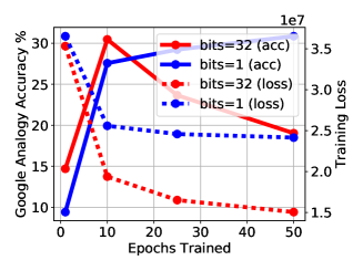
(a) Training loss and accuracy vs epochs trained (vector dimension = 400) on 100MB of Wikipedia. Trends show that Word2Vec is prone to overfitting with many epochs of training.

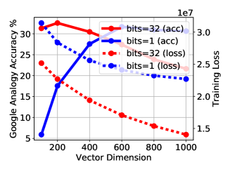
(b) Training loss and accuracy vs dimension (epochs trained = 10) on 100MB of Wikipedia. Trends show that overfitting may occur with larger vector dimensions.

Figure 1: Overfitting in full precision Word2Vec training; regularization in quantized Word2vec training

4.4 Word2Bits Visualization

Figure 2 shows a visualization of 800 dimensional 1 bit word vectors trained on English Wikipedia (2017). The top 100 closest and furthest word vectors to the target word vector are plotted. Distance is measured by dot product; every 5 word vectors are labelled. A turquoise line separates the 100 closest vectors to the target word from the 100 furthest vectors (labelled “…”). We see that there are qualitative similarities between word vectors whose words are related to each other.

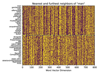
(a)

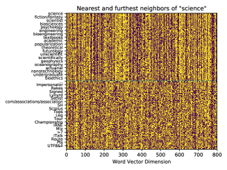
(b)

(c)

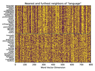
(d)

(e)

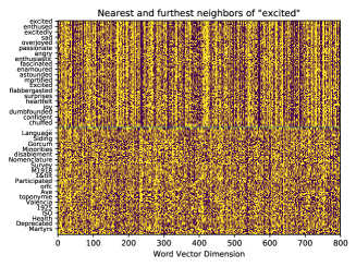
(f)

Figure 2: Visualizing 1-bit 800 dimensional word vectors

5 Conclusion and Future Work

In this report we have shown that it is possible to train high quality quantized vectors that take 8-16x less storage/memory than full precision vectors. Interestingly, quantized word vectors perform better than full precision vectors on both word similarity and question answering, but worse on word analogy. The data suggest that performing well on word analogy tasks require a higher number of bits per word while doing well on word similarity tasks require fewer. Another interesting observation is that performance on the intrinsic tasks did not really predict performance on extrinsic tasks (SQuAD) – this validates the findings of [3, 12]. We have also shown that full precision Word2Vec training is prone to overfitting (across training epochs and across word vector dimension) on smaller datasets (100MB of Wikipedia); this suggests it is not always better to train for many epochs. We believe the same phenomena holds for larger datasets. A final interesting observation is that parameter values of Word2Vec vectors tend to “explode” with higher dimensions, an issue that virtually quantized training does not have. This suggests it may be helpful to introduce a regularization term to Word2Vec.

Future work involves evaluating full precision vectors and quantized vectors on other extrinsic tasks, which will give a more complete picture of the relative performance of the two. We would also like to train quantized word vectors on much larger corpuses of data such as Common Crawl or Google News. Another task is to validate that overfitting occurs on larger datasets (full English Wikipedia) with respect to various tasks (other intrinsic tasks, extrinsic tasks). Finally, we believe it is possible to do virtually quantized training with Glove, though initial experiments suggest that several modifications to the loss function are needed to make it work.

Acknowledgments

Huge thanks to Sen Wu, Christopher Aberger, Kevin Clark and Professors Richard Socher and Christopher Ré for their advice and assistance on the project!

References

[1] Armand Joulin, Edouard Grave, Piotr Bojanowski, Matthijs Douze, Herve Jegou, and Tomas Mikolov. 2016. Fast-text.zip: Compressing text classification models. arXiv preprint arXiv:1612.03651.

[2] Armand Joulin, Edouard Grave, Piotr Bojanowski, and Tomas Mikolov. 2016. Bag of tricks for efficient text classification. arXiv preprint arXiv:1607.01759.

[3] Billy Chiu, Anna Korhonen, and Sampo Pyysalo. 2016. Intrinsic evaluation of word vectors fails to predict extrinsic performance. Proceedings of RepEval 2016.

[4] Omer Levy, Yoav Goldberg, and Ido Dagan. 2015. Improving distributional similarity with lessons learned from word embeddings. TACL.

[5] Y. LeCun, J. S. Denker, S. Solla, R. E. Howard, and L. D. Jackel. Optimal brain damage. In Advances in Neural Information Processing Systems, pages 598-605, 1990.

[6] Han, Song, Pool, Jeff, Tran, John, and Dally, William J. Learning both weights and connections for efficient neural networks. In Advances in Neural Information Processing Systems, 2015.

[7] Tomas Mikolov, Ilya Sutskever, Kai Chen, Greg Corrado, and Jeff Dean. 2013. Distributed representations of words and phrases and their compositionality. In Advances in Neural Information Processing Systems 26, pages 3111-3119.

[8] Tomas Mikolov, Kai Chen, Greg Corrado, and Jeffrey Dean. Efficient estimation of word representations in vector space. In International Conference on Learning Representations: Workshops Track, 2013. arxiv.org/abs/1301.3781.

[9] Courbariaux, M., Hubara, I., Soudry, D., El-Yaniv, R., and Bengio, Y. Binarized Neural Networks: Training Deep Neural Networks with Weights and Activations Constrained to +1 or -1. arXiv preprint arXiv:1602.02830, 2016.

[10] Hinton, Geoffrey. Neural networks for machine learning. Coursera, video lectures, 2012.

[11] Pennington, Jeffrey, Richard Socher, and Christopher D Manning. 2014. Glove: Global vectors for word representation. Proceedings of the Empiricial Methods in Natural Language Processing (EMNLP 2014) 12.

[12] Tobias Schnabel, Igor Labutov, David Mimno, and Thorsten Joachims. 2015. Evaluation methods for unsupervised word embeddings. In Proc. of EMNLP.

[13] P. Rajpurkar, J. Zhang, K. Lopyrev, and P. Liang. Squad: 100,000+ questions for machine comprehension of text. In Empirical Methods in Natural Language Processing (EMNLP), 2016.

[14] Chen, D.; Fisch, A.; Weston, J.; and Bordes, A. 2017. Reading wikipedia to answer open-domain questions. arXiv preprint arXiv:1704.00051

[15] Lev Finkelstein, Evgeniy Gabrilovich, Yossi Matias, Ehud Rivlin, Zach Solan, Gadi Wolfman, and Eytan Ruppin. 2002. Placing search in context: The concept revisited. ACM Transactions on Information Systems, 20(1):116-131.

[16] Torsten Zesch, Christof Muller, and Iryna Gurevych. 2008. Using wiktionary for computing semantic relatedness. In Proceedings of the 23rd National Conference on Artificial Intelligence - Volume 2, AAAI’08, pages 861-866. AAAI Press.

[17] Eneko Agirre, Enrique Alfonseca, Keith Hall, Jana Kravalova, Marius Pasca, and Aitor Soroa. 2009. A study on similarity and relatedness using distributional and wordnet-based approaches. In Proceedings of Human Language Technologies: The 2009 Annual Conference of the North American Chapter of the Association for Computational Linguistics, pages 19-27, Boulder, Colorado, June. Association for Computational Linguistics.

[18] Elia Bruni, Gemma Boleda, Marco Baroni, and Nam Khanh Tran. 2012. Distributional semantics in technicolor. In Proceedings of the 50th Annual Meeting of the Association for Computational Linguistics (Volume 1: Long Papers), pages 136-145, Jeju Island, Korea, July. Association for Computational Linguistics.

[19] Kira Radinsky, Eugene Agichtein, Evgeniy Gabrilovich, and Shaul Markovitch. 2011. A word at a time: Computing word relatedness using temporal semantic analysis. In Proceedings of the 20th international conference on World wide web, pages 337-346. ACM.

[20] Minh-Thang Luong, Richard Socher, and Christopher D. Manning. 2013. Better word representations with recursive neural networks for morphology. In Proceedings of the Seventeenth Conference on Computational Natural Language Learning, pages 104-113, Sofia, Bulgaria, August. Association for Computational Linguistics.

[21] Roi Reichart Felix Hill and Anna Korhonen. 2014. Simlex-999: Evaluating semantic models with (genuine) similarity estimation. arXiv preprint arXiv:1408.3456.

[22] Courbariaux, M., Bengio, Y., David, J.P.: Training deep neural networks with low precision multiplications. arXiv preprint arXiv:1412.7024 (2014)

[23] W. Chen, J. T. Wilson, S. Tyree, K. Q. Weinberger, and Y. Chen, “Compressing neural networks with the hashing trick,” in International Conference on Machine Learning (ICML), 2015, pp. 2285-2294.

[24] Abigail See, Minh-Thang Luong, and Christopher D. Manning. 2016. Compression of Neural Machine Translation via Pruning. In Proceedings of CoNLL.

[25] Raphael Shu, Hideki Nakayama. 2017. Compressing Word Embeddings via Deep Compositional Code Learning. In International Conference on Learning Representations, 2017.

[26] Christopher De Sa, Megan Leszczynski, Jian Zhang, Alana Marzoev, Christopher R. Aberger, Kunle Olukotun, Christopher Ré. 2018. High-Accuracy Low-Precision Training. arXiv preprint arXiv:1803.03383

[27] Bryan McCann, James Bradbury, Caiming Xiong, and Richard Socher. Learned in translation: Contextualized word vectors. In NIPS, 2017.

[28] Neelakantan, Arvind, Vilnis, Luke, Le, Quoc V., Sutskever, Ilya, Kaiser, Lukasz, Kurach, Karol, and Martens, James. Adding gradient noise improves learning for very deep networks. ICLR Workshop, 2016.

[29] Hinton, G. Vinyals, O. and Dean, J. Distilling knowledge in a neural network. In Deep Learning and Representation Learning Workshop, NIPS, 2014.

[30] Bengio, Yoshua. Estimating or propagating gradients through stochastic neurons. Technical Report arXiv:1305.2982, Universite de Montreal, 2013.

[31] Matt Mahoney. About the test data, 2011. URL http://mattmahoney.net/dc/textdata.

[32] B. Hassibi, D. Stork, G. Wolff and T. Watanabe. Optimal brain surgeon: Extensions and performance comparisons. In Advances in Neural Information Processing Systems 6. Morgan Kaufman, San Mateo, CA: 263-270, 1994.