Proximal SCOPE for distributed sparse learning: Better data partition implies faster convergence rate

Abstract

Distributed sparse learning with a cluster of multiple machines has attracted much attention in machine learning, especially for large-scale applications with high-dimensional data. One popular way to implement sparse learning is to use $L_{1}$ regularization. In this paper, we propose a novel method, called proximal SCOPE (pSCOPE), for distributed sparse learning with $L_{1}$ regularization. pSCOPE is based on a cooperative autonomous local learning (CALL) framework. In the CALL framework of pSCOPE, we find that the data partition affects the convergence of the learning procedure, and subsequently we define a metric to measure the goodness of a data partition. Based on the defined metric, we theoretically prove that pSCOPE is convergent with a linear convergence rate if the data partition is good enough. We also prove that better data partition implies faster convergence rate. Furthermore, pSCOPE is also communication efficient. Experimental results on real data sets show that pSCOPE can outperform other state-of-the-art distributed methods for sparse learning.

1 Introduction

Many machine learning models can be formulated as the following regularized empirical risk minimization problem:

$$\mathop{\min}_{{\bf w}\in{\mathbb{R}}^{d}}~{}P({\bf w})=\frac{1}{n}\sum_{i=1}^{n}f_{i}({\bf w})+R({\bf w}),$$ (1)

where ${\bf w}$ is the parameter to learn, $f_{i}({\bf w})$ is the loss on training instance $i$, $n$ is the number of training instances, and $R({\bf w})$ is a regularization term. Recently, sparse learning, which tries to learn a sparse model for prediction, has become a hot topic in machine learning. There are different ways to implement sparse learning [30, 32]. One popular way is to use $L_{1}$ regularization, i.e., $R({\bf w})=\lambda\|{\bf w}\|_{1}$. In this paper, we focus on sparse learning with $R({\bf w})=\lambda\|{\bf w}\|_{1}$. Hence, in the following content of this paper, $R({\bf w})=\lambda\|{\bf w}\|_{1}$ unless otherwise stated.

One traditional method to solve (1) is proximal gradient descent (pGD) [2], which can be written as follows:

$${\bf w}_{t+1}=\mbox{prox}_{R,\eta}({\bf w}_{t}-\eta\nabla F({\bf w}_{t})),$$ (2)

where $F({\bf w})=\frac{1}{n}\sum_{i=1}^{n}f_{i}({\bf w})$, ${\bf w}_{t}$ is the value of ${\bf w}$ at iteration $t$, $\eta$ is the learning rate, $prox$ is the proximal mapping defined as

$$\mbox{prox}_{R,\eta}({\bf u})=\mathop{\arg\min}_{{\bf v}}(R({\bf v})+\frac{1}{2\eta}\|{\bf v}-{\bf u}\|^{2}).$$ (3)

Recently, stochastic learning methods, including stochastic gradient descent (SGD) [19], stochastic average gradient (SAG) [23], stochastic variance reduced gradient (SVRG) [10], and stochastic dual coordinate ascent (SDCA) [26], have been proposed to speedup the learning procedure in machine learning. Inspired by the success of these stochastic learning methods, proximal stochastic methods, including proximal SGD (pSGD) [12, 6, 28, 4], proximal block coordinate descent (pBCD) [31, 33, 22], proximal SVRG (pSVRG) [34] and proximal SDCA (pSDCA) [27], have also been proposed for sparse learning in recent years. All these proximal stochastic methods are sequential (serial) and implemented with one single thread.

The serial proximal stochastic methods may not be efficient enough for solving large-scale sparse learning problems. Furthermore, the training set might be distributively stored on a cluster of multiple machines in some applications. Hence, distributed sparse learning [1] with a cluster of multiple machines has attracted much attention in recent years, especially for large-scale applications with high-dimensional data. In particular, researchers have recently proposed several distributed proximal stochastic methods for sparse learning [16, 18, 14, 17, 29].

One main branch of the distributed proximal stochastic methods includes distributed pSGD (dpSGD) [16], distributed pSVRG (dpSVRG) [9, 18] and distributed SVRG (DSVRG) [14]. Both dpSGD and dpSVRG adopt a centralized framework and mini-batch based strategy for distributed learning. One typical implementation of a centralized framework is based on Parameter Server [15, 35], which supports both synchronous and asynchronous communication strategies. One shortcoming of dpSGD and dpSVRG is that the communication cost is high. More specifically, the communication cost of each epoch is $O(n)$, where $n$ is the number of training instances. DSVRG adopts a decentralized framework with lower communication cost than dpSGD and dpSVRG. However, in DSVRG only one worker is updating parameters locally and all other workers are idling at the same time.

Another branch of the distributed proximal stochastic methods is based on block coordinate descent [3, 21, 7, 17]. Although in each iteration these methods update only a block of coordinates, they usually have to pass through the whole data set. Due to the partition of data, it also brings high communication cost in each iteration.

Another branch of the distributed proximal stochastic methods is based on SDCA. One representative is PROXCOCOA$+$ [29]. Although PROXCOCOA$+$ has been theoretically proved to have a linear convergence rate with low communication cost, we find that it is not efficient enough in experiments.

In this paper, we propose a novel method, called proximal SCOPE (pSCOPE), for distributed sparse learning with $L_{1}$ regularization. pSCOPE is a proximal generalization of the scalable composite optimization for learning (SCOPE) [36]. SCOPE cannot be used for sparse learning, while pSCOPE can be used for sparse learning. The contributions of pSCOPE are briefly summarized as follows:

• pSCOPE is based on a cooperative autonomous local learning (CALL) framework. In the CALL framework, each worker in the cluster performs autonomous local learning based on the data assigned to that worker, and the whole learning task is completed by all workers in a cooperative way. The CALL framework is communication efficient because there is no communication during the inner iterations of each epoch.

• pSCOPE is theoretically guaranteed to be convergent with a linear convergence rate if the data partition is good enough, and better data partition implies faster convergence rate. Hence, pSCOPE is also computation efficient.

• In pSCOPE, a recovery strategy is proposed to reduce the cost of proximal mapping when handling high dimensional sparse data.

• Experimental results on real data sets show that pSCOPE can outperform other state-of-the-art distributed methods for sparse learning.

2 Preliminary

In this paper, we use $\|\cdot\|$ to denote the $L_{2}$ norm $\|\cdot\|_{2}$, ${\bf w}^{*}$ to denote the optimal solution of (1). For a vector ${\bf a}$, we use $a^{(j)}$ to denote the $j$th coordinate value of ${\bf a}$. $[n]$ denotes the set $\{1,2,\ldots,n\}$. For a function $h({\bf a};{\bf b})$, we use $\nabla h({\bf a};{\bf b})$ to denote the gradient of $h({\bf a};{\bf b})$ with respect to (w.r.t.) the first argument ${\bf a}$. Furthermore, we give the following definitions.

Definition 1

We call a function $h(\cdot)$ is $L$-smooth if it is differentiable and there exists a positive constant $L$ such that $\forall{\bf a},{\bf b}:h({\bf b})\leq h({\bf a})+\nabla h({\bf a})^{T}({\bf b}-{\bf a})+\frac{L}{2}\|{\bf a}-{\bf b}\|^{2}$.

Definition 2

We call a function $h(\cdot)$ is convex if there exists a constant $\mu\geq 0$ such that $\forall{\bf a},{\bf b}:h({\bf b})\geq h({\bf a})+\zeta^{T}({\bf b}-{\bf a})+\frac{\mu}{2}\|{\bf a}-{\bf b}\|^{2}$, where $\zeta\in\partial h({\bf a})=\{{\bf c}|h({\bf b})\geq h({\bf a})+{\bf c}^{T}({\bf b}-{\bf a}),\forall{\bf a},{\bf b}\}$. If $h(\cdot)$ is differentiable, then $\zeta=\nabla h({\bf a})$. If $\mu>0$, $h(\cdot)$ is called $\mu$-strongly convex.

Throughout this paper, we assume that $R({\bf w})$ is convex, $F({\bf w})=\frac{1}{n}\sum_{i=1}^{n}f_{i}({\bf w})$ is strongly convex and each $f_{i}({\bf w})$ is smooth. We do not assume that each $f_{i}({\bf w})$ is convex.

3 Proximal SCOPE

In this paper, we focus on distributed learning with one master (server) and $p$ workers in the cluster, although the algorithm and theory of this paper can also be easily extended to cases with multiple servers like the Parameter Server framework [15, 35].

The parameter ${\bf w}$ is stored in the master, and the training set $D=\{{\bf x}_{i},y_{i}\}_{i=1}^{n}$ are partitioned into $p$ parts denoted as $D_{1},D_{2},\ldots,D_{p}$. Here, $D_{k}$ contains a subset of instances from $D$, and $D_{k}$ will be assigned to the $k$th worker. $D=\bigcup_{k=1}^{p}D_{k}$. Based on this data partition scheme, the proximal SCOPE (pSCOPE) for distributed sparse learning is presented in Algorithm 1. The main task of master is to add and average vectors received from workers. Specifically, it needs to calculate the full gradient ${\bf z}=\nabla F({\bf w}_{t})=\frac{1}{n}\sum_{k=1}^{p}{\bf z}_{k}$. Then it needs to calculate ${\bf w}_{t+1}=\frac{1}{p}\sum_{k=1}^{p}{\bf u}_{k,M}$. The main task of workers is to update the local parameters ${\bf u}_{1,m},{\bf u}_{2,m},\ldots,{\bf u}_{p,m}$ initialized with ${\bf u}_{k,0}={\bf w}_{t}$. Specifically, for each worker $k$, after it gets the full gradient ${\bf z}$ from master, it calculates a stochastic gradient

$${\bf v}_{k,m}=\nabla f_{i_{k,m}}({\bf u}_{k,m})-\nabla f_{i_{k,m}}({\bf w}_{t})+{\bf z},$$ (4)

and then update its local parameter ${\bf u}_{k,m}$ by a proximal mapping with learning rate $\eta$:

$${\bf u}_{k,m+1}=\mbox{prox}_{R,\eta}({\bf u}_{k,m}-\eta{\bf v}_{k,m}).$$ (5)

Algorithm 1 Proximal SCOPE

1:  Initialize ${\bf w}_{0}$ and the learning rate $\eta$;

2:  Task of master:

3:  for $t=0,1,2,...T-1$ do

4:     Send ${\bf w}_{t}$ to each worker;

5:     Wait until receiving ${\bf z}_{1},{\bf z}_{2},\ldots,{\bf z}_{p}$ from all workers;

6:     Calculate the full gradient ${\bf z}=\frac{1}{n}\sum_{k=1}^{p}{\bf z}_{k}$ and send ${\bf z}$ to each worker;

7:     Wait until receiving ${\bf u}_{1,M},{\bf u}_{2,M},\ldots,{\bf u}_{p,M}$ from all workers and calculate ${\bf w}_{t+1}=\frac{1}{p}\sum_{k=1}^{p}{\bf u}_{k,M}$;

8:  end for

9:  Task of the $k$th worker:

10:  for $t=0,1,2,...T-1$ do

11:     Wait until receiving ${\bf w}_{t}$ from master;

12:     Let ${\bf u}_{k,0}={\bf w}_{t}$, calculate ${\bf z}_{k}=\sum_{i\in D_{k}}f_{i}({\bf w}_{t})$ and send ${\bf z}_{k}$ to master;

13:     Wait until receiving ${\bf z}$ from master;

14:     for $m=0,1,2,...M-1$ do

15:        Randomly choose an instance ${\bf x}_{i_{k,m}}\in D_{k}$;

16:        Calculate ${\bf v}_{k,m}=\nabla f_{i_{k,m}}({\bf u}_{k,m})-\nabla f_{i_{k,m}}({\bf w}_{t})+{\bf z}$;

17:        Update ${\bf u}_{k,m+1}=\mbox{prox}_{R,\eta}({\bf u}_{k,m}-\eta{\bf v}_{k,m})$;

18:     end for

19:     Send ${\bf u}_{k,M}$ to master

20:  end for

From Algorithm 1, we can find that pSCOPE is based on a cooperative autonomous local learning (CALL) framework. In the CALL framework, each worker in the cluster performs autonomous local learning based on the data assigned to that worker, and the whole learning task is completed by all workers in a cooperative way. The cooperative operation is mainly adding and averaging in the master. During the autonomous local learning procedure in each outer iteration which contains $M$ inner iterations (see Algorithm 1), there is no communication. Hence, the communication cost for each epoch of pSCOPE is constant, which is much less than the mini-batch based strategy with $O(n)$ communication cost for each epoch [16, 9, 18].

pSCOPE is a proximal generalization of SCOPE [36]. Although pSCOPE is mainly motivated by sparse learning with $L_{1}$ regularization, the algorithm and theory of pSCOPE can also be used for smooth regularization like $L_{2}$ regularization. Furthermore, when the data partition is good enough, pSCOPE can avoid the extra term $c({\bf u}_{k,m}-{\bf w}_{t})$ in the update rule of SCOPE, which is necessary for convergence guarantee of SCOPE.

4 Effect of Data Partition

In our experiment, we find that the data partition affects the convergence of the learning procedure. Hence, in this section we propose a metric to measure the goodness of a data partition, based on which the convergence of pSCOPE can be theoretically proved. Due to space limitation, the detailed proof of Lemmas and Theorems are moved to the long version [37].

4.1 Partition

First, we give the following definition:

Definition 3

Define $\pi=[\phi_{1}(\cdot),\ldots,\phi_{p}(\cdot)]$. We call $\pi$ a partition w.r.t. $P(\cdot)$, if $F({\bf w})=\frac{1}{p}\sum_{k=1}^{p}\phi_{k}({\bf w})$ and each $\phi_{k}(\cdot)~{}(k=1,\ldots,p)$ is $\mu_{k}$-strongly convex and $L_{k}$-smooth ($\mu_{k},L_{k}>0$). Here, $P(\cdot)$ is defined in (1) and $F(\cdot)$ is defined in (2). We denote $A(P)=\{\pi|\pi$ is a partition w.r.t. $P(\cdot)\}$.

Remark 1

Here, $\pi$ is an ordered sequence of functions. In particular, if we construct another partition $\pi{{}^{\prime}}$ by permuting $\phi_{i}(\cdot)$ of $\pi$, we consider them to be two different partitions. Furthermore, two functions $\phi_{i}(\cdot),\phi_{j}(\cdot)~{}(i\neq j)$ in $\pi$ can be the same. Two partitions $\pi_{1}=[\phi_{1}(\cdot),\ldots,\phi_{p}(\cdot)]$, $\pi_{2}=[\psi_{1}(\cdot),\ldots,\psi_{p}(\cdot)]$ are considered to be equal, i.e., $\pi_{1}=\pi_{2}$, if and only if $\phi_{k}({\bf w})=\psi_{k}({\bf w})(k=1,\ldots,p),\forall{\bf w}$.

For any partition $\pi=[\phi_{1}(\cdot),\ldots,\phi_{p}(\cdot)]$ w.r.t. $P(\cdot)$, we construct new functions $P_{k}(\cdot;\cdot)$ as follows:

$$P_{k}({\bf w};{\bf a})=\phi_{k}({\bf w};{\bf a})+R({\bf w}),k=1,\ldots,p$$ (6)

where $\phi_{k}({\bf w};{\bf a})=\phi_{k}({\bf w})+G_{k}({\bf a})^{T}{\bf w}$, $G_{k}({\bf a})=\nabla F({\bf a})-\nabla\phi_{k}({\bf a})$, and ${\bf w},{\bf a}\in{\mathbb{R}}^{d}$.

In particular, given a data partition $D_{1},D_{2},\ldots,D_{p}$ of the training set $D$, let $F_{k}({\bf w})=\frac{1}{|D_{k}|}\sum_{i\in D_{k}}f_{i}({\bf w})$ which is also called the local loss function. Assume each $F_{k}(\cdot)$ is strongly convex and smooth, and $F({\bf w})=\frac{1}{p}\sum_{k=1}^{p}F_{k}({\bf w})$. Then, we can find that $\pi=[F_{1}(\cdot),\ldots,F_{p}(\cdot)]$ is a partition w.r.t. $P(\cdot)$. By taking expectation on ${\bf v}_{k,m}$ defined in Algorithm 1, we obtain ${\mathbb{E}}[{\bf v}_{k,m}|{\bf u}_{k,m}]=\nabla F_{k}({\bf u}_{k,m})+G_{k}({\bf w}_{t})$. According to the theory in [34], in the inner iterations of pSCOPE, each worker tries to optimize the local objective function $P_{k}({\bf w};{\bf w}_{t})$ using proximal SVRG with initialization ${\bf w}={\bf w}_{t}$ and training data $D_{k}$, rather than optimizing $F_{k}({\bf w})+R({\bf w})$. Then we call such a $P_{k}({\bf w};{\bf a})$ the local objective function w.r.t. $\pi$. Compared to the subproblem of PROXCOCOA$+$ (equation (2) in [29]), $P_{k}({\bf w};{\bf a})$ is more simple and there is no hyperparameter in it.

4.2 Good Partition

In general, the data distribution on each worker is different from the distribution of the whole training set. Hence, there exists a gap between each local optimal value and the global optimal value. Intuitively, the whole learning algorithm has slow convergence rate or cannot even converge if this gap is too large.

Definition 4

For any partition $\pi$ w.r.t. $P(\cdot)$, we define the Local-Global Gap as

$$l_{\pi}({\bf a})=P({\bf w}^{*})-\frac{1}{p}\sum_{k=1}^{p}P_{k}({\bf w}_{k}^{*}({\bf a});{\bf a}),$$

where ${\bf w}_{k}^{*}({\bf a})=\mathop{\arg\min}_{{\bf w}}P_{k}({\bf w};{\bf a})$.

We have the following properties of Local-Global Gap:

Lemma 1

$\forall\pi\in A(P)$, $l_{\pi}({\bf a})=P({\bf w}^{*})+\frac{1}{p}\sum_{k=1}^{p}H_{k}^{*}(-G_{k}({\bf a}))\geq l_{\pi}({\bf w}^{*})=0,\forall{\bf a}$, where $H_{k}^{*}(\cdot)$ is the conjugate function of $\phi_{k}(\cdot)+R(\cdot)$.

Theorem 1

Let $R({\bf w})=\|{\bf w}\|_{1}$. $\forall\pi\in A(P)$, there exists a constant $\gamma<\infty$ such that $l_{\pi}({\bf a})\leq\gamma\|{\bf a}-{\bf w}^{*}\|^{2},\forall{\bf a}$.

The result in Theorem 1 can be easily extended to smooth regularization which can be found in the long version [37].

According to Theorem 1, the local-global gap can be bounded by $\gamma\|{\bf a}-{\bf w}^{*}\|^{2}$. Given a specific ${\bf a}$, the smaller $\gamma$ is, the smaller the local-global gap will be. Since the constant $\gamma$ only depends on the partition $\pi$, intuitively $\gamma$ can be used to evaluate the goodness of a partition $\pi$. We define a good partition as follows:

Definition 5

We call $\pi$ a $(\epsilon,\xi)$-good partition w.r.t. $P(\cdot)$ if $\pi\in A(P)$ and

$$\gamma(\pi;\epsilon)\overset{\triangle}{=}\mathop{sup}_{\|{\bf a}-{\bf w}^{*}\|^{2}\geq\epsilon}\frac{l_{\pi}({\bf a})}{\|{\bf a}-{\bf w}^{*}\|^{2}}\leq\xi.$$ (7)

In the following, we give the bound of $\gamma(\pi;\epsilon)$.

Lemma 2

Assume $\pi=[F_{1}(\cdot),\ldots,F_{p}(\cdot)]$ is a partition w.r.t. $P(\cdot)$, where $F_{k}({\bf w})=\frac{1}{|D_{k}|}\sum_{i\in D_{k}}f_{i}({\bf w})$ is the local loss function, each $f_{i}(\cdot)$ is Lipschitz continuous with bounded domain and sampled from some unknown distribution ${\mathbb{P}}$. If we assign these $\{f_{i}(\cdot)\}$ uniformly to each worker, then with high probability, $\gamma(\pi;\epsilon)\leq\frac{1}{p}\sum_{k=1}^{p}\mathcal{O}(1/(\epsilon\sqrt{|D_{k}|}))$. Moreover, if $l_{\pi}({\bf a})$ is convex w.r.t. ${\bf a}$, then $\gamma(\pi;\epsilon)\leq\frac{1}{p}\sum_{k=1}^{p}\mathcal{O}(1/\sqrt{\epsilon|D_{k}|})$. Here we ignore the $\log$ term and dimensionality $d$.

For example, in Lasso regression, it is easy to get that the corresponding local-global gap $l_{\pi}({\bf a})$ is convex according to Lemma 1 and the fact that $G_{k}({\bf a})$ is an affine function in this case.

Lemma 2 implies that as long as the size of training data is large enough, $\gamma(\pi;\epsilon)$ will be small and $\pi$ will be a good partition. Please note that the uniformly here means each $f_{i}(\cdot)$ will be assigned to one of the $p$ workers and each worker has the equal probability to be assigned. We call the partition resulted from uniform assignment uniform partition in this paper. With uniform partition, each worker will have almost the same number of instances. As long as the size of training data is large enough, uniform partition is a good partition.

5 Convergence of Proximal SCOPE

In this section, we will prove the convergence of Algorithm 1 for proximal SCOPE (pSCOPE) using the results in Section 4.

Theorem 2

Assume $\pi=[F_{1}(\cdot),\ldots,F_{p}(\cdot)]$ is a $(\epsilon,\xi)$-good partition w.r.t. $P(\cdot)$. For convenience, we set $\mu_{k}=\mu,L_{k}=L,k=1,2\ldots,p$. If $\|{\bf w}_{t}-{\bf w}^{*}\|^{2}\geq\epsilon$, then

$${\mathbb{E}}\|{\bf w}_{t+1}-{\bf w}^{*}\|^{2}\leq[(1-\mu\eta+2L^{2}\eta^{2})^{M}+\frac{2L^{2}\eta+2\xi}{\mu-2L^{2}\eta}]\|{\bf w}_{t}-{\bf w}^{*}\|^{2}.$$

Because smaller $\xi$ means better partition and the partition $\pi$ corresponds to data partition in Algorithm 1, we can see that better data partition implies faster convergence rate.

Corollary 1

Assume $\pi=[F_{1}(\cdot),\ldots,F_{p}(\cdot)]$ is a $(\epsilon,\frac{\mu}{8})$-good partition w.r.t. $P(\cdot)$. For convenience, we set $\mu_{k}=\mu,L_{k}=L,k=1,2\ldots,p$. If $\|{\bf w}_{t}-{\bf w}^{*}\|^{2}\geq\epsilon$, taking $\eta=\frac{\mu}{12L^{2}}$, $M=20\kappa^{2}$, where $\kappa=\frac{L}{\mu}$ is the conditional number, then we have ${\mathbb{E}}\|{\bf w}_{t+1}-{\bf w}^{*}\|^{2}\leq\frac{3}{4}\|{\bf w}_{t}-{\bf w}^{*}\|^{2}$. To get the $\epsilon$-suboptimal solution, the computation complexity of each worker is $O((n/p+\kappa^{2})\log(\frac{1}{\epsilon}))$.

Corollary 2

When $p=1$, which means we only use one worker, pSCOPE degenerates to proximal SVRG [34]. Assume $F(\cdot)$ is $\mu$-strongly convex ($\mu>0$) and $L$-smooth. Taking $\eta=\frac{\mu}{6L^{2}}$, $M=13\kappa^{2}$, we have ${\mathbb{E}}\|{\bf w}_{t+1}-{\bf w}^{*}\|^{2}\leq\frac{3}{4}\|{\bf w}_{t}-{\bf w}^{*}\|^{2}$. To get the $\epsilon$-optimal solution, the computation complexity is $O((n+\kappa^{2})\log(\frac{1}{\epsilon}))$.

We can find that pSCOPE has a linear convergence rate if the partition is $(\epsilon,\xi)$-good, which implies pSCOPE is computation efficient and we need $T=O(\log(\frac{1}{\epsilon}))$ outer iterations to get a $\epsilon$-optimal solution. For all inner iterations, each worker updates ${\bf u}_{k,m}$ without any communication. Hence, the communication cost is $O(\log(\frac{1}{\epsilon}))$, which is much smaller than the mini-batch based strategy with $O(n)$ communication cost for each epoch [16, 9, 18].

Furthermore, in the above theorems and corollaries, we only assume that the local loss function $F_{k}(\cdot)$ is strongly convex. We do not need each $f_{i}(\cdot)$ to be convex. Hence, $M=O(\kappa^{2})$ and it is weaker than the assumption in proximal SVRG [34] whose computation complexity is $O((n+\kappa)\log(\frac{1}{\epsilon}))$ when $p=1$. In addition, without convexity assumption for each $f_{i}(\cdot)$, our result for the degenerate case $p=1$ is consistent with that in [24].

6 Handle High Dimensional Sparse Data

For the cases with high dimensional sparse data, we propose recovery strategy to reduce the cost of proximal mapping so that it can accelerate the training procedure. Here, we adopt the widely used linear model with elastic net [38] as an example for illustration, which can be formulated as follows: $\mathop{\min}_{{\bf w}}P({\bf w}):=\frac{1}{n}\sum_{i=1}^{n}h_{i}({\bf x}_{i}^{T}{\bf w})+\frac{\lambda_{1}}{2}\|{\bf w}\|^{2}+\lambda_{2}\|{\bf w}\|_{1}$, where $h_{i}:{\mathbb{R}}\rightarrow{\mathbb{R}}$ is the loss function. We assume many instances in $\{{\bf x}_{i}\in{\mathbb{R}}^{d}|i\in[n]\}$ are sparse vectors and let $C_{i}=\{j|x_{i}^{(j)}\neq 0\}$.

Proximal mapping is unacceptable when the data dimensionality $d$ is too large, since we need to execute the conditional statements $O(Md)$ times which is time consuming. Other methods, like proximal SGD and proximal SVRG, also suffer from this problem.

Since $z^{(j)}$ is a constant during the update of local parameter ${\bf u}_{k,m}$, we will design a recovery strategy to recover it when necessary. More specifically, in each inner iteration, with the random index $s=i_{k,m}$, we only recover $u^{(j)}$ to calculate the inner product ${\bf x}_{s}^{T}{\bf u}_{k,m}$ and update $u^{(j)}_{k,m}$ for $j\in C_{s}$. For those $j\notin C_{s}$, we do not immediately update $u^{(j)}_{k,m}$. The basic idea of these recovery rules is: for some coordinate $j$, we can calculate $u_{k,m_{2}}^{(j)}$ directly from $u_{k,m_{1}}^{(j)}$, rather than doing iterations from $m=m_{1}$ to $m_{2}$. Here, $0\leq m_{1}<m_{2}\leq M$. At the same time, the new algorithm is totally equivalent to Algorithm 1. It will save about $O(d(m_{2}-m_{1})(1-\rho))$ times of conditional statements, where $\rho$ is the sparsity of $\{{\bf x}_{i}\in{\mathbb{R}}^{d}|i\in[n]\}$. This reduction of computation is significant especially for high dimensional sparse training data. Due to space limitation, the complete rules are moved to the long version [37]. Here we only give one case of our recovery rules in Lemma 3.

Lemma 3

(Recovery Rule) We define the sequence $\{\alpha_{q}\}$ as: $\alpha_{0}=0$ and for $q=1,2,\ldots$, $\alpha_{q}=\sum_{i=1}^{q}(1-\lambda_{1}\eta)^{i-1}/(1-\lambda_{1}\eta)^{q}$. For the coordinate $j$ and constants $m_{1},m_{2}$, if $j\notin C_{i_{k,m}}$ for any $m\in[m_{1},m_{2}-1]$. If $|z^{(j)}|<\lambda_{2},u_{k,m_{1}}^{(j)}>0$, then the relation between $u_{k,m_{1}}^{(j)}$ and $u_{k,m_{2}}^{(j)}$ can be summarized as follows: define $q_{0}$ which satisfies $\alpha_{q_{0}}\eta(z^{(j)}+\lambda_{2})\leq u_{k,m_{1}}^{(j)}<\alpha_{q_{0}+1}\eta(z^{(j)}+\lambda_{2}),$

1. If $m_{2}-m_{1}\leq q_{0}$, then $u_{k,m_{2}}^{(j)}=(1-\lambda_{1}\eta)^{m_{2}-m_{1}}[u_{k,m_{1}}^{(j)}-\alpha_{m_{2}-m_{1}}\eta(z^{(j)}+\lambda_{2})].$

2. If $m_{2}-m_{1}>q_{0}$, then $u_{k,m_{2}}^{(j)}=0.$

7 Experiment

We use two sparse learning models for evaluation. One is logistic regression (LR) with elastic net [38]: $P({\bf w})=\frac{1}{n}\sum_{i=1}^{n}\log(1+e^{-y_{i}{\bf x}_{i}^{T}{\bf w}})+\frac{\lambda_{1}}{2}\|{\bf w}\|^{2}+\lambda_{2}\|{\bf w}\|_{1}$. The other is Lasso regression [30]: $P({\bf w})=\frac{1}{2n}\sum_{i=1}^{n}({\bf x}_{i}^{T}{\bf w}-y_{i})^{2}+\lambda_{2}\|{\bf w}\|_{1}$. All experiments are conducted on a cluster of multiple machines. The CPU for each machine has 12 Intel E5-2620 cores, and the memory of each machine is 96GB. The machines are connected by 10GB Ethernet. Evaluation is based on four datasets in Table 1: cov, rcv1, avazu, kdd2012. All of them can be downloaded from LibSVM website .

Table 1: Datasets

	#instances	#features	$\lambda_{1}$	$\lambda_{2}$
cov	581,012	54	$10^{-5}$	$10^{-5}$
rcv1	677,399	47,236	$10^{-5}$	$10^{-5}$
avazu	23,567,843	1,000,000	$10^{-7}$	$10^{-5}$
kdd2012	119,705,032	54,686,452	$10^{-8}$	$10^{-5}$

7.1 Baselines

We compare our pSCOPE with six representative baselines: proximal gradient descent based method FISTA [2], ADMM type method DFAL [1], newton type method mOWL-QN [8], proximal SVRG based method AsyProx-SVRG [18], proximal SDCA based method PROXCOCOA$+$ [29], and distributed block coordinate descent DBCD [17]. FISTA and mOWL-QN are serial. We design distributed versions of them, in which workers distributively compute the gradients and then master gathers the gradients from workers for parameter update.

All methods use 8 workers. One master will be used if necessary. Unless otherwise stated, all methods except DBCD and PROXCOCOA$+$ use the same data partition, which is got by uniformly assigning each instance to each worker (uniform partition). Hence, different workers will have almost the same number of instances. This uniform partition strategy satisfies the condition in Lemma 2. Hence, it is a good partition. DBCD and PROXCOCOA$+$ adopt a coordinate distributed strategy to partition the data.

7.2 Results

The convergence results of LR with elastic net and Lasso regression are shown in Figure 1. DBCD is too slow, and hence we will separately report the time of it and pSCOPE when they get $10^{-3}$-suboptimal solution in Table 2. AsyProx-SVRG is slow on the two large datasets avazu and kdd2012, and hence we only present the results of it on the datasets cov and rcv1. From Figure 1 and Table 2, we can find that pSCOPE outperforms all the other baselines on all datasets.

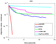
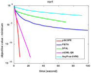
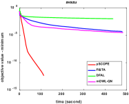
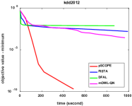
(a) LR with elastic net

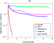
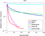
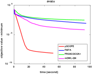
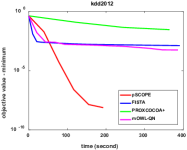
(b) Lasso regression

Figure 1: Evaluation with baselines on two models.

Table 2: Time comparison (in second) between pSCOPE and DBCD.

		pSCOPE	DBCD
	cov	0.32	822
LR	rcv1	3.78	$>1000$
	cov	0.06	81.9
Lasso	rcv1	3.09	$>1000$

7.3 Speedup

We also evaluate the speedup of pSCOPE on the four datasets for LR. We run pSCOPE and stop it when the gap $P({\bf w})-P({\bf w}^{*})\leq 10^{-6}$. The speedup is defined as: ${\mbox{Speedup}}=(\mbox{Time using one worker})/(\mbox{Time using }p\mbox{ workers})$. We set $p=1,2,4,8$. The speedup results are in Figure 2 (a). We can find that pSCOPE gets promising speedup.

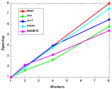
(a) Speedup of pSCOPE

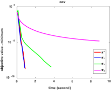
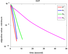
(b) Effect of data partition

Figure 2: Speedup and effect of data partition

7.4 Effect of Data Partition

We evaluate pSCOPE under different data partitions. We use two datasets cov and rcv1 for illustration, since they are balanced datasets which means the number of positive instances is almost the same as that of negative instances. For each dataset, we construct four data partitions: $\pi^{*}$ (Each worker has access to the whole data), $\pi_{1}$ (Uniform partition); $\pi_{2}$ (75% positive instances and 25% negative instances are on the first 4 workers, and other instances are on the last 4 workers), $\pi_{3}$ (All positive instances are on the first 4 workers, and all negative instances are on the last 4 workers).

The convergence results are shown in Figure 2 (b). We can see that data partition does affect the convergence of pSCOPE. The partition $\pi^{*}$ achieves the best performance, which verifies the theory in this paper . The performance of uniform partition $\pi_{1}$ is similar to that of the best partition $\pi^{*}$, and is better than the other two data partitions. In real applications with large-scale dataset, it is impractical to assign each worker the whole dataset. Hence, we prefer to choose uniform partition $\pi_{1}$ in real applications, which is also adopted in above experiments of this paper.

8 Conclusion

In this paper, we propose a novel method, called pSCOPE, for distributed sparse learning. Furthermore, we theoretically analyze how the data partition affects the convergence of pSCOPE. pSCOPE is both communication and computation efficient. Experiments on real data show that pSCOPE can outperform other state-of-the-art methods to achieve the best performance.

Appendix A Effect of Data Partition

A.1 Proof of Lemma 1

$\forall\pi\in A(P)$, $l_{\pi}({\bf a})=P({\bf w}^{*})+\frac{1}{p}\sum_{k=1}^{p}H_{k}^{*}(-G_{k}({\bf a}))\geq l_{\pi}({\bf w}^{*})=0,\forall{\bf a}$, where $H_{k}^{*}(\cdot)$ is the conjugate function of $\phi_{k}(\cdot)+R(\cdot)$.

Proof  According to Definition 4 and ${\bf w}_{k}^{*}({\bf a})$, we have

$$l_{\pi}({\bf a})= P({\bf w}^{*})-\frac{1}{p}\sum_{i=1}^{p}P_{k}({\bf w}_{k}^{*}({\bf a});{\bf a})$$

$$= \frac{1}{p}\sum_{i=1}^{p}(P_{k}({\bf w}^{*};{\bf a})-P({\bf w}_{k}^{*}({\bf a});{\bf a}))\geq 0$$

On the other hand, let ${\bf a}={\bf w}^{*}$, then ${\bf w}_{k}^{*}({\bf w}^{*})=\mathop{\arg\min}_{\bf w}P_{k}({\bf w};{\bf w}^{*})$, and

$$\nabla\phi_{k}({\bf w}^{*};{\bf w}^{*})+\zeta$$

$$= \nabla\phi_{k}({\bf w}^{*})+\nabla F({\bf w}^{*})-\nabla\phi_{k}({\bf w}^{*})+\zeta$$

$$= \nabla F({\bf w}^{*})+\zeta$$

$$= {\bf 0}$$

where $\zeta\in\partial R({\bf w}^{*})$ so that $\nabla F({\bf w}^{*})+\zeta={\bf 0}$. It implies that ${\bf w}^{*}=\mathop{\arg\min}_{\bf w}P_{k}({\bf w};{\bf w}^{*})$. Due to the strong convexity of $P_{k}({\bf w};{\bf w}^{*})$ w.r.t ${\bf w}$, we have ${\bf w}_{k}^{*}({\bf w}^{*})={\bf w}^{*}$, which means $l_{\pi}({\bf w}^{*})=0$.

For the dual form, according to (6) and definition of ${\bf w}_{k}^{*}({\bf y})$, we have

$$P({\bf w}_{k}^{*}({\bf a});{\bf a})= \mathop{\min}_{\bf w}(\phi_{k}({\bf w})+R({\bf w})+G_{k}({\bf a})^{T}{\bf w}))$$

$$= -\mathop{\max}_{\bf w}(-G_{k}({\bf a})^{T}{\bf w}-(\phi_{k}({\bf w})+R({\bf w})))$$

$$= -H_{k}^{*}(-G_{k}({\bf a}))$$

Then we have

$$l_{\pi}({\bf a})=P({\bf w}^{*})+\frac{1}{p}\sum_{k=1}^{p}H_{k}^{*}(-G_{k}({\bf a}))$$

$\square$

A.2 Proof of Theorem 1

A.2.1 Warm up: quadratic function

We start with the simple quadratic function in one dimension space that

$$\phi_{k}(w)=\frac{1}{2}m_{k}w^{2}+b_{k}w+c_{k},$$

and

$$F(w)=\frac{1}{2}mw^{2}+bw+c,R(w)=|w|,$$

where $w,m_{k},b_{k},c_{k}\in{\mathbb{R}},m_{k}>0$, and $\frac{1}{p}\sum_{k=1}^{p}m_{k}=m,\frac{1}{p}\sum_{k=1}^{p}b_{k}=b,\frac{1}{p}\sum_{k=1}^{p}c_{k}=c$ so that $\pi=[\phi_{1}(\cdot),\ldots,\phi_{p}(\cdot)]\in A(P)$. The corresponding $P_{k}(\cdot;\cdot)$ is defined as

$$P_{k}(w;a)= \frac{1}{2}m_{k}w^{2}+b_{k}w+c_{k}+(ma+b-m_{k}a-b_{k})w+|w|$$

$$= \frac{1}{2}m_{k}w^{2}+(ma+b-m_{k}a)w+c_{k}+|w|$$ (8)

Then we have the following lemma:

Lemma 4

With $\phi_{k}(\cdot),F(\cdot),R(\cdot)$ defined above,

$$P(w^{*})-\frac{1}{p}\sum_{k=1}^{p}P_{k}(w_{k}^{*}(a);a)\leq\gamma(a-w^{*})^{2},\forall a\in{\mathbb{R}}$$

where $\gamma=\frac{1}{p}\sum_{k=1}^{p}\frac{(m-m_{k})^{2}}{m_{k}}$.

Proof  For convenience, we define three sets

$$K_{1}(a)=\{k|(m-m_{k})y+b<-1\}$$

$$K_{2}(a)=\{k|(m-m_{k})y+b\in[-1,1]\}$$

$$K_{3}(a)=\{k|(m-m_{k})y+b>1\}$$

Then it is easy to find that

• if $k\in K_{1}(a)$, then $w_{k}^{*}(a)=-\frac{(m-m_{k})a+b+1}{m_{k}}$, $P_{k}(w_{k}^{*}(a);a)=-\frac{[(m-m_{k})a+b+1]^{2}}{2m_{k}}+c_{k}$;

• if $k\in K_{2}(a)$, then $w_{k}^{*}(a)=0$, $P_{k}(w_{k}^{*}(a);a)=c_{k}$;

• if $k\in K_{3}(a)$, then $w_{k}^{*}(a)=-\frac{(m-m_{k})a+b-1}{m_{k}}$, $P_{k}(w_{k}^{*}(a);a)=-\frac{[(m-m_{k})a+b-1]^{2}}{2m_{k}}+c_{k}$;

Now we calculate the Local-Global Gap.

Firstly we consider the case that $b<-1$, we have $w^{*}=-\frac{b+1}{m}$, $P(w^{*})=-\frac{(b+1)^{2}}{2m}+c$, and

$$l_{\pi}(y)= -\frac{(b+1)^{2}}{2m}-\frac{1}{p}[\sum_{k\in K_{1}(a)}-\frac{[(m-m_{k})a+b+1]^{2}}{2m_{k}}$$

$$+\sum_{k\in K_{3}(a)}-\frac{[(m-m_{k})a+b-1]^{2}}{2m_{k}}]$$

$$= -\frac{mw^{*2}}{2}+\frac{1}{p}[\sum_{k\in K_{1}(a)}\frac{[(m-m_{k})a-mw^{*}]^{2}}{2m_{k}}$$

$$+\sum_{k\in K_{3}(a)}\frac{[(m-m_{k})a-mw^{*}-2]^{2}}{2m_{k}}]$$

For $k\in K_{3}(a)$, we have

$$[(m-m_{k})a-mw^{*}-2]^{2}$$

$$= [(m-m_{k})a-mw^{*}]^{2}-4[(m-m_{k})a-mw^{*}]+4$$

$$= [(m-m_{k})a-mw^{*}]^{2}-4[(m-m_{k})a+b+1]+4$$

$$\leq [(m-m_{k})a-mw^{*}]^{2}$$

Then we have

$$l_{\pi}(a)\leq -\frac{mw^{*2}}{2}+\frac{1}{p}[\sum_{k\in K_{1}(a)}\frac{[(m-m_{k})a-mw^{*}]^{2}}{2m_{k}}$$

$$+\sum_{k\in K_{3}(a)}\frac{[(m-m_{k})a-mw^{*}]^{2}}{2m_{k}}]$$

$$\leq -\frac{mw^{*2}}{2}+\frac{1}{p}\sum_{k=1}^{p}\frac{[(m-m_{k})a-mw^{*}]^{2}}{2m_{k}}$$

$$= \frac{1}{p}\sum_{k=1}^{p}\frac{(m-m_{k})^{2}}{m_{k}}(a-w^{*})^{2}$$

Secondly we consider the case that $b\in[-1,1]$, we have $w^{*}=0$, $P(w^{*})=c$, and

$$l_{\pi}(a)= \frac{1}{p}[\sum_{k\in K_{1}(a)}\frac{[(m-m_{k})a+b+1]^{2}}{2m_{k}}$$

$$+\sum_{k\in K_{3}(a)}\frac{[(m-m_{k})a+b-1]^{2}}{2m_{k}}]$$

For $k\in K_{1}(a)$, we have $(m-m_{k})a<-(b+1)\leq 0$, which means that $[(m-m_{k})a]^{2}>(b+1)^{2}$. Then we have

$$[(m-m_{k})a+b+1]^{2}$$

$$= [(m-m_{k})a]^{2}+(b+1)^{2}+2(b+1)(m-m_{k})a$$

$$\leq 2[(m-m_{k})a]^{2}$$

For $k\in K_{3}(a)$, with the similar reason, we have

$$[(m-m_{k})a+b-1]^{2}$$

$$= [(m-m_{k})a]^{2}+(b-1)^{2}+2(b-1)(m-m_{k})a$$

$$\leq 2[(m-m_{k})a]^{2}$$

Then we have

$$l_{\pi}(a)\leq \frac{1}{p}[\sum_{k\in K_{1}(a)}\frac{2[(m-m_{k})a]^{2}}{2m_{k}}+\sum_{k\in K_{3}(a)}\frac{2[(m-m_{k})a]^{2}}{2m_{k}}]$$

$$\leq \frac{1}{p}\sum_{k=1}^{p}\frac{2[(m-m_{k})a]^{2}}{2m_{k}}$$

$$= \frac{1}{p}\sum_{k=1}^{p}\frac{(m-m_{k})^{2}}{m_{k}}(a-w^{*})^{2}$$

For the case $b<-1$, it is the same as that $b<-1$. We have $l_{\pi}(a)\leq\frac{1}{p}\sum_{k=1}^{p}\frac{(m-m_{k})^{2}}{m_{k}}(a-w^{*})^{2}$. $\square$

So that any $\pi$ is a qualified partition in this case. In high dimension space with diagonal positive definite matrices, we can also get similar result:

Lemma 5

Let $\phi_{k}({\bf w})=\frac{1}{2}{\bf w}^{T}{\bf A}_{k}{\bf w}+{\bf b}_{k}^{T}{\bf w}+c_{k}$, $F({\bf w})=\frac{1}{2}{\bf w}^{T}{\bf A}{\bf w}+{\bf b}^{T}{\bf w}+c$, $R({\bf w})=\|{\bf w}\|_{1}$, where ${\bf A}_{k},{\bf A}\in{\mathbb{R}}^{d\times d}$ are diagonal positive definite matrices, ${\bf x},{\bf b},{\bf b}_{k}\in{\mathbb{R}}^{d},d>1$ and $c_{k},c\in{\mathbb{R}}$ and $[\phi_{1}(\cdot),\phi_{2}(\cdot),\ldots,\phi_{p}(\cdot)]\in A(P)$. With $\gamma=\mathop{\max}_{i=1,\ldots,d}\frac{1}{p}\sum_{k=1}^{p}\frac{(A(i,i)-A_{k}(i,i))^{2}}{A_{k}(i,i)}$, where $A(i,i)$, $A_{k}(i,i)$ are the $i^{th}$ diagonal elements of ${\bf A},{\bf A}_{k}$ respectively, then we have

$$P({\bf w}^{*})-\frac{1}{p}\sum_{k=1}^{p}P_{k}({\bf w}_{k}^{*}({\bf a});{\bf a})\leq\gamma\|{\bf a}-{\bf w}^{*}\|^{2},\forall{\bf a}\in{\mathbb{R}}^{d}.$$

One can find that although the local objective function in (A.2.1) is non-smooth, the corresponding local-global gap is differentiable at $w^{*}$. This is not surprise. In fact, for any partition $\pi=[\phi_{1}(\cdot),\ldots,\phi_{p}(\cdot)]$, according to the dual form in Lemma 1 and the duality of strong convexity [11], we obtain the following lemma:

Lemma 6

Let $\phi_{k}({\bf w})=\frac{1}{2}{\bf w}^{T}{\bf A}_{k}{\bf w}+{\bf b}_{k}^{T}{\bf w}+c_{k}$, $F({\bf w})=\frac{1}{2}{\bf w}^{T}{\bf A}{\bf w}+{\bf b}^{T}{\bf w}+c$, $R({\bf w})=\|{\bf w}\|_{1}$, where ${\bf A}_{k},{\bf A}\in{\mathbb{R}}^{d\times d}$ are positive definite matrices, ${\bf w},{\bf b},{\bf b}_{k}\in{\mathbb{R}}^{d},d>1$ , $c_{k},c\in{\mathbb{R}}$ and $[\phi_{1}(\cdot),\phi_{2}(\cdot),\ldots,\phi_{p}(\cdot)]\in A(P)$. then there must exist $\gamma$ such that

$$P({\bf w}^{*})-\frac{1}{p}\sum_{k=1}^{p}P_{k}({\bf w}_{k}^{*}({\bf a});{\bf a})\leq\gamma\|{\bf a}-{\bf w}^{*}\|^{2},\forall{\bf a}\in{\mathbb{R}}^{d}.$$

Proof  Since $\phi_{k}({\bf w})+R({\bf w})$ is strongly convex, the corresponding conjugate function is smooth. Noting that $G_{k}({\bf a})$ is an affine function, we have $H_{k}^{*}(-G_{k}({\bf a}))$ is smooth as well, which means $l_{\pi}({\bf a})$ is smooth w.r.t ${\bf a}$. Then according to Lemma 1, we have $l_{\pi}({\bf w}^{*})=0,\nabla l_{\pi}({\bf w}^{*})={\bf 0}$. With Definition 1, there must exist $\gamma>0$ such that $l_{\pi}({\bf a})\leq\gamma\|{\bf a}-{\bf w}^{*}\|^{2},\forall{\bf a}$. $\square$

A.2.2 Extension to general $\phi_{k}(\cdot)$

Below, we will consider the general case. To evaluate $l_{\pi}({\bf a})$ for general $\phi_{k}(\cdot)$, we consider the Taylor expansion of $\phi_{k}(\cdot)$ using its smoothness:for any fixed ${\bf w}_{0}$, let

$$\tilde{\phi}_{k,{\bf w}_{0}}({\bf w})$$

$$= \phi_{k}({\bf w}_{0})+\nabla\phi_{k}({\bf w}_{0})^{T}({\bf w}-{\bf w}_{0})+\frac{\mu_{k}}{2}\|{\bf w}-{\bf w}_{0}\|^{2}$$ (9)

$$\hat{\phi}_{k,{\bf w}_{0}}({\bf w})$$

$$= \phi_{k}({\bf w}_{0})+\nabla\phi_{k}({\bf w}_{0})^{T}({\bf w}-{\bf w}_{0})+\frac{L_{k}}{2}\|{\bf w}-{\bf w}_{0}\|^{2}$$ (10)

which are two quadratic functions satisfy the condition of Lemma 5. By the smooth and strong convex property of $\phi_{k}(\cdot)$, we have $\tilde{\phi}_{k,{\bf w}_{0}}({\bf w})\leq\phi_{k}({\bf w})\leq\hat{\phi}_{k,{\bf w}_{0}}({\bf w}),\forall{\bf w}$. Now we proof the theorem:

Let $R({\bf w})=\|{\bf w}\|_{1}$. $\forall\pi\in A(P)$, there exists constant $\gamma<\infty$ such that $l_{\pi}({\bf a})\leq\gamma\|{\bf a}-{\bf w}^{*}\|^{2},\forall{\bf a}$.

Proof  We define

$$\tilde{\phi}_{k,{\bf w}_{0}}({\bf w};{\bf a}) =\tilde{\phi}_{k,{\bf w}_{0}}({\bf w})+(\nabla\tilde{\phi}_{{\bf w}_{0}}({\bf a})-\nabla\tilde{\phi}_{k,{\bf w}_{0}}({\bf a}))^{T}{\bf w}$$

$$\tilde{P}_{k,{\bf w}_{0}}({\bf w};{\bf a}) =\tilde{\phi}_{k,{\bf w}_{0}}({\bf w};{\bf a})+R({\bf w})$$

where $\tilde{\phi}_{{\bf w}_{0}}({\bf a})=\frac{1}{p}\sum_{k=1}^{p}\tilde{\phi}_{k,{\bf w}_{0}}({\bf a})$. It is easy to find that taking ${\bf a}={\bf w}_{0}$,

$$\tilde{P}_{k,{\bf w}_{0}}({\bf w};{\bf w}_{0})$$

$$= \tilde{\phi}_{k,{\bf w}_{0}}({\bf w})+(\nabla\tilde{\phi}_{{\bf w}_{0}}({\bf w}_{0})-\nabla\tilde{\phi}_{k,{\bf w}_{0}}({\bf w}_{0}))^{T}{\bf w}+R({\bf w})$$

$$= \tilde{\phi}_{k,{\bf w}_{0}}({\bf w})+(\nabla F({\bf w}_{0})-\nabla\phi_{k}({\bf w}_{0}))^{T}{\bf w}+R({\bf w})$$

$$\leq \phi_{k}({\bf w})+G_{k}({\bf w}_{0})^{T}{\bf w}+R({\bf w})$$

$$= P_{k}({\bf w};{\bf w}_{0})$$

where $G_{k}(\cdot),P_{k}(\cdot;\cdot)$ is defined in (6). It implies that

$$-\min_{{\bf w}}P_{k}({\bf w};{\bf w}_{0})\leq-\min_{{\bf w}}\tilde{P}_{k,{\bf w}_{0}}({\bf w};{\bf w}_{0})$$ (11)

Since $\tilde{\phi}_{k,{\bf w}_{0}}({\bf w})$, defined in (9), is quadratic function w.r.t ${\bf w}$ that satisfied the condition in Lemma 5, there must exist a constant $\gamma_{1}$ (note that the constant $\gamma_{1}$ is independent on ${\bf w}_{0}$) such that $\forall{\bf a}$,

$$\mathop{\min}_{{\bf w}}\tilde{P}_{{\bf w}_{0}}({\bf w})-\frac{1}{p}\sum_{k=1}^{p}\mathop{\min}_{{\bf w}}\tilde{P}_{k,{\bf w}_{0}}({\bf w};{\bf a})\leq\gamma_{1}\|{\bf a}-\tilde{{\bf w}}^{*}({\bf w}_{0})\|^{2},$$ (12)

where $\tilde{P}_{{\bf w}_{0}}({\bf w})=\frac{1}{p}\sum_{k=1}^{p}\tilde{\phi}_{k,{\bf w}_{0}}({\bf w})+R({\bf w})$, $\tilde{{\bf w}}^{*}({\bf w}_{0})=\mathop{\arg\min}_{\bf w}\tilde{P}_{{\bf w}_{0}}({\bf w})$.

Furthermore, by defining $\hat{P}_{{\bf w}_{0}}({\bf w})=\frac{1}{p}\sum_{k=1}^{p}\hat{\phi}_{k,{\bf w}_{0}}({\bf w})+R({\bf w})$, where $\hat{\phi}_{k,{\bf w}_{0}}({\bf w})$ is defined in (10), we get that

$$P({\bf w})\leq\hat{P}_{{\bf w}_{0}}({\bf w}),\forall{\bf w}$$ (13)

Taking ${\bf a}={\bf w}_{0}$ in (12), $\bar{L}=\frac{1}{p}\sum_{i=k}^{p}L_{k},\bar{\mu}=\frac{1}{p}\sum_{i=k}^{p}\mu_{k}$, we obtain

$$P({\bf w}^{*})-\frac{1}{p}\sum_{k=1}^{p}\mathop{\min}_{{\bf w}}P_{k}({\bf w};{\bf w}_{0})$$

$$= P({\bf w}^{*})-\tilde{P}_{{\bf w}_{0}}(\tilde{{\bf w}}^{*}({\bf w}_{0}))+\tilde{P}_{{\bf w}_{0}}(\tilde{{\bf w}}^{*}({\bf w}_{0}))-\frac{1}{p}\sum_{k=1}^{p}\mathop{\min}_{{\bf w}}P_{k}({\bf w};{\bf w}_{0})$$

$$\overset{(\ref{eq:the_1.1})}{\leq} P({\bf w}^{*})-\tilde{P}_{{\bf w}_{0}}(\tilde{{\bf w}}^{*}({\bf w}_{0}))+\tilde{P}_{{\bf w}_{0}}(\tilde{{\bf w}}^{*}({\bf w}_{0}))-\frac{1}{p}\sum_{k=1}^{p}\mathop{\min}_{{\bf w}}\tilde{P}_{k,{\bf w}_{0}}({\bf w};{\bf w}_{0})$$

$$\overset{(\ref{eq:the_1.2})}{\leq} P({\bf w}^{*})-\tilde{P}_{{\bf w}_{0}}(\tilde{{\bf w}}^{*}({\bf w}_{0}))+\gamma_{1}\|{\bf w}_{0}-\tilde{{\bf w}}^{*}({\bf w}_{0})\|^{2}$$

$$\leq P(\tilde{{\bf w}}^{*}({\bf w}_{0}))-\tilde{P}_{{\bf w}_{0}}(\tilde{{\bf w}}^{*}({\bf w}_{0}))+\gamma_{1}\|{\bf w}_{0}-\tilde{{\bf w}}^{*}({\bf w}_{0})\|^{2}$$

$$\overset{(\ref{eq:the_1.3})}{\leq} \hat{P}_{{\bf w}_{0}}(\tilde{{\bf w}}^{*}({\bf w}_{0}))-\tilde{P}_{{\bf w}_{0}}(\tilde{{\bf w}}^{*}({\bf w}_{0}))+\gamma_{1}\|{\bf w}_{0}-\tilde{{\bf w}}^{*}({\bf w}_{0})\|^{2}$$

$$= (\frac{\bar{L}-\bar{\mu}}{2}+\gamma_{1})\|{\bf w}_{0}-\tilde{{\bf w}}^{*}({\bf w}_{0})\|^{2}$$

$$\leq (\bar{L}-\bar{\mu}+2\gamma_{1})(\|{\bf w}_{0}-{\bf w}^{*}\|^{2}+\|{\bf w}^{*}-\tilde{{\bf w}}^{*}({\bf w}_{0})\|^{2})$$

$$= (\bar{L}-\bar{\mu}+2\gamma_{1})(\|{\bf w}_{0}-{\bf w}^{*}\|^{2}+\|\tilde{{\bf w}}^{*}({\bf w}^{*})-\tilde{{\bf w}}^{*}({\bf w}_{0})\|^{2})$$

where the last inequality using the fact that $\tilde{{\bf w}}^{*}({\bf w}^{*})={\bf w}^{*}$. Using Lemma 7, which clarifies the Lipschitz continuity of $\tilde{{\bf w}}^{*}(\cdot)$, we get that there must exist some constant $\gamma$ such that

$$P({\bf w}^{*})-\frac{1}{p}\sum_{k=1}^{p}\mathop{\min}_{{\bf w}}P_{k}({\bf w};{\bf w}_{0})\leq\gamma\|{\bf w}_{0}-{\bf w}^{*}\|^{2}$$ (14)

$\square$

We denote $\tilde{{\bf w}}^{*}({\bf w}_{0})=\mathop{\arg\min}_{{\bf w}}\tilde{P}_{{\bf w}_{0}}({\bf w})$, $\bar{L}=\frac{1}{p}\sum_{i=k}^{p}L_{k},\bar{\mu}=\frac{1}{p}\sum_{i=k}^{p}\mu_{k}$. We have the following lemma:

Lemma 7

$\tilde{{\bf w}}^{*}({\bf w})$ is Lipschitz continue w.r.t ${\bf w}$.

Proof  We use $w^{(i)}$ to denote the $i^{th}$ element of ${\bf w}$ and define $\psi^{i}({\bf w})=\bar{\mu}w^{(i)}-(\nabla F({\bf w}))^{(i)}$. Since $\nabla F({\bf w})$ is Lipschitz continue, so as $\psi^{i}({\bf w})$ (assume it is $\alpha$-Lipschitz continue). We define three sets $A^{i}=\{{\bf w}|\psi^{i}({\bf w})>1\},B^{i}=\{{\bf w}|\psi^{i}({\bf w})\in[-1,1]\},C^{i}=\{{\bf w}|\psi^{i}({\bf w})<-1\}$. According to the definition of $\tilde{P}_{{\bf w}}({\bf x})$, which is a quadratic function, we have

$$(\tilde{{\bf w}}^{*}({\bf w}))^{(i)}= \frac{1}{\bar{\mu}}(\psi^{i}({\bf w})-1),\mbox{if }{\bf w}\in A^{i}$$

$$(\tilde{{\bf w}}^{*}({\bf w}))^{(i)}= 0,\mbox{if }{\bf w}\in B^{i}$$

$$(\tilde{{\bf w}}^{*}({\bf w}))^{(i)}= \frac{1}{\bar{\mu}}(\psi^{i}({\bf w})+1),\mbox{if }{\bf w}\in C^{i}$$

First it is easy to note that $(\tilde{{\bf w}}^{*}({\bf w}))^{(i)}$ is Lipschitz continue w.r.t ${\bf w}$ on $A^{i},B^{i},C^{i}$ respectively and is continue w.r.t ${\bf w}$ on the whole domain. Second, we take three points ${\bf w}_{1}\in A^{i},{\bf w}_{2}\in B^{i},{\bf w}_{3}\in C^{i}$. Since $\psi^{i}({\bf w})$ is continue w.r.t ${\bf w}$ on the whole domain, there must be $\theta_{12},\theta_{13},\theta_{23}\in[0,1]$ such that $\psi^{i}(\theta_{12}{\bf w}_{1}+(1-\theta_{12}){\bf w}_{2})=1,\psi^{i}(\theta_{13}{\bf w}_{1}+(1-\theta_{13}){\bf w}_{3})\in B^{i},\psi^{i}(\theta_{23}{\bf w}_{2}+(1-\theta_{23}){\bf w}_{3})=-1$. It implies that

$$|(\tilde{{\bf w}}^{*}({\bf w}_{1}))^{(i)}-(\tilde{{\bf w}}^{*}({\bf w}_{2}))^{(i)}|$$

$$= \frac{1}{\bar{\mu}}(\psi^{i}({\bf w}_{1})-1)$$

$$= \frac{1}{\bar{\mu}}(\psi^{i}({\bf w}_{1})-\psi^{i}(\theta_{12}{\bf w}_{1}+(1-\theta_{12}){\bf w}_{2}))$$

$$\leq \frac{\alpha(1-\theta_{12})}{\bar{\mu}}\|{\bf w}_{1}-{\bf w}_{2}\|$$

$$\leq \frac{\alpha}{\bar{\mu}}\|{\bf w}_{1}-{\bf w}_{2}\|$$

Similarly we can find that $|(\tilde{{\bf w}}^{*}({\bf w}_{1}))^{(i)}-(\tilde{{\bf w}}^{*}({\bf w}_{3}))^{(i)}|\leq\frac{\alpha}{\bar{\mu}}\|{\bf w}_{1}-{\bf w}_{3}\|$, $|(\tilde{{\bf w}}^{*}({\bf w}_{2}))^{(i)}-(\tilde{{\bf w}}^{*}({\bf w}_{3}))^{(i)}|\leq\frac{\alpha}{\bar{\mu}}\|{\bf w}_{2}-{\bf w}_{3}\|$. So $(\tilde{{\bf w}}^{*}({\bf w}))^{(i)}$ is Lipschitz continue. It implies that $\tilde{{\bf w}}^{*}({\bf w})$ is Lipschitz continue w.r.t ${\bf w}$. $\square$

The result in Theorem 1 can be easily extended to smooth regularization:

Theorem 3

Let $R(\cdot)$ be smooth. $\forall\pi\in A(P)$, there exists constant $\gamma<\infty$ such that

$$l_{\pi}({\bf a})\leq\gamma\|{\bf a}-{\bf w}^{*}\|,\forall{\bf a}.$$

Proof  Since $R({\bf w})$ is smooth, so as $P_{k}({\bf w};{\bf a})$ w.r.t ${\bf w}$, then there exist some constant $L{{}^{\prime}}$ (independent on ${\bf a}$) such that

$$l_{\pi}({\bf a})= \frac{1}{p}\sum_{k=1}^{p}P_{k}({\bf w}^{*};{\bf a})-P_{k}({\bf w}_{k}^{*}({\bf a});{\bf a})$$

$$\leq \frac{1}{p}\sum_{k=1}^{p}\frac{L{{}^{\prime}}}{2}\|{\bf w}^{*}-{\bf w}_{k}^{*}({\bf a})\|^{2}$$

Here we use the fact $P({\bf w}^{*})=\frac{1}{p}\sum_{k=1}^{p}P_{k}({\bf w}^{*};{\bf a})$ and $\nabla P_{k}({\bf w}_{k}^{*}({\bf a});{\bf a})=0$. On the other hand, we have

$$\nabla\phi_{k}({\bf w}_{k}^{*}({\bf a}))+\nabla F({\bf a})-\nabla\phi_{k}({\bf a})+\nabla R({\bf w}_{k}^{*}({\bf a}))=0$$

$$\nabla F({\bf w}^{*})+\nabla R({\bf w}^{*})=0$$

which means that

$$\|\nabla\phi_{k}({\bf w}_{k}^{*}({\bf a}))+\nabla R({\bf w}_{k}^{*}({\bf a}))-\nabla\phi_{k}({\bf w}^{*})-\nabla R({\bf w}^{*})\|$$

$$= \|\nabla\phi_{k}({\bf a})-\nabla\phi_{k}({\bf w}^{*})-\nabla R({\bf w}^{*})-\nabla F({\bf a})\|$$

$$= \|\nabla\phi_{k}({\bf a})-\nabla\phi_{k}({\bf w}^{*})+\nabla F({\bf w}^{*})-\nabla F({\bf a})\|$$

By strong convexity of $\phi_{k}({\bf w})+R({\bf w})$, smoothness of $\phi_{k}({\bf w})$, $F({\bf w})$, we have

$$\|{\bf w}^{*}-{\bf w}_{k}^{*}({\bf a})\|\leq\frac{L_{k}+L}{\mu_{k}}\|{\bf a}-{\bf w}^{*}\|$$

So there must be some constant $\gamma$ such that $l_{\pi}({\bf a})\leq\gamma\|{\bf a}-{\bf w}^{*}\|^{2}$. $\square$

A.3 Condition of continuity of $\gamma(\pi;0)$

Let $\pi^{*}=[F(\cdot),\ldots,F(\cdot)]$, where $F(\cdot)=\frac{1}{n}\sum_{i=1}^{n}f_{i}(\cdot)$ is defined in (1). We can find that $\pi^{*}$ is the best partition since $l_{\pi^{*}}({\bf a})=0,\forall{\bf a}$, which implies

$$\gamma(\pi^{*};0)=0$$

In the following content, we will prove that $\gamma(\pi;\epsilon)\rightarrow 0$ as $\pi$ approaches $\pi^{*}$. We first define the distance between two partitions as follows:

Definition 6

Let $\pi_{1}=[\phi_{1}(\cdot),\ldots,\phi_{p}(\cdot)]$ and $\pi_{2}=[\psi_{1}(\cdot),\ldots,\psi_{p}(\cdot)]$ be two partitions w.r.t. $P(\cdot)$, the distance between $\pi_{1}$ and $\pi_{2}$ is

$$d(\pi_{1},\pi_{2})=\mathop{\max}_{i=1,\ldots,p}\{\mathop{\sup}_{{\bf w}}|\phi_{i}({\bf w})-\psi_{i}({\bf w})|,\mathop{\sup}_{{\bf w}}\|\nabla\phi_{i}({\bf w})-\nabla\psi_{i}({\bf w})\|\}.$$

We can prove that it is a reasonable definition of distance. For convenience, we assume the domain of these $\phi_{k}(\cdot)$ and $\psi_{k}(\cdot)$ is closed and bounded, which is denoted as $\mathcal{W}=\{{\bf w}|\|{\bf w}\|\leq B\}$ and ${\bf w}^{*}\in\mathcal{W}$. Hence, $d(\pi_{1},\pi_{2})<\infty$.

With the definition of distance between two partitions, we have

Lemma 8

Let $\pi=[\phi_{1}(\cdot),\ldots,\phi_{p}(\cdot)]$ be a partition w.r.t. $P(\cdot)$. $l_{\pi}({\bf a})$ uniformly converges to $l_{\pi^{*}}({\bf a})=0$ as $d(\pi,\pi^{*})\rightarrow 0$.

Besides the uniform convergence of $l_{\pi}({\bf a})$ w.r.t. $\pi$, we also prefer the uniform convergence of $\gamma(\pi;\epsilon)$ w.r.t. $\pi$ since it reflects the goodness of partition $\pi$. According to the definition of $\gamma(\pi;\epsilon)$, it easy to note that $\gamma(\pi;0)\geq\gamma(\pi;\epsilon),\forall\epsilon\geq 0$. Below, we would like to explore the necessary and sufficient condition of continuity of $\gamma(\pi;0)$ at $\pi^{*}$. For convenience, we only consider one dimension space, which means $d=1$(In high dimension space, similar result could be got). We assume $l_{\pi}(a)\in C^{3}(\mathcal{W},{\mathbb{R}})$ (note that $\mathcal{W}$ is compact).

Lemma 9

If $\lim_{\pi\to\pi^{*}}\gamma(\pi;0)=0$, then $l_{\pi}^{{}^{\prime\prime}}(w^{*})$ converge to $l_{\pi^{*}}^{{}^{\prime\prime}}(w^{*})=0$.

Proof  If it is wrong, there must exist partitions $\{\pi_{n}\}$ and constant $a$ such that $l_{\pi_{n}}^{{}^{\prime\prime}}(w^{*})>a>0$ (or $<a<0$), and $d(\pi_{n},\pi_{*})\rightarrow 0$ as $n\rightarrow\infty$. Since $l_{\pi_{n}}(w^{*})=l_{\pi_{n}}^{{}^{\prime}}(w^{*})=0$, then for the series $\{y_{n}\}$ with $y_{n}=w^{*}+\frac{1}{n\sup_{x}{|l_{\pi_{n}}^{{}^{\prime\prime\prime}}(x)}|}$, by Taylor theory, we obtain:

$$l_{\pi_{n}}(y_{n})=\frac{1}{2}l_{\pi_{n}}^{{}^{\prime\prime}}(w^{*})(y_{n}-w^{*})^{2}+\frac{1}{6}l_{\pi_{n}}^{{}^{\prime\prime\prime}}(\zeta_{n})(y_{n}-w^{*})^{3}$$

which implies

$$\gamma(\pi_{n};0)\geq \frac{1}{2}l_{\pi_{n}}^{{}^{\prime\prime}}(w^{*})+\frac{1}{6}l_{\pi_{n}}^{{}^{\prime\prime\prime}}(\zeta_{n})(y_{n}-w^{*})$$

$$> \frac{a}{2}+\frac{l_{\pi_{n}}^{{}^{\prime\prime\prime}}(\zeta_{n})}{6n\sup_{x}{|l_{\pi_{n}}^{{}^{\prime\prime\prime}}(x)}|}$$

Let $n\rightarrow\infty$, it conflicts with the condition. $\square$

For the necessary and sufficient condition, we have the following result:

Lemma 10

$\lim_{\pi\to\pi^{*}}\gamma(\pi;0)=0$ if and only if there exist some $\delta$ such that $l_{\pi}^{{}^{\prime\prime}}(y)$ uniformly converge to $l_{\pi^{*}}^{{}^{\prime\prime}}(y)=0$ on $\{y||y-w^{*}|<\delta\}$ w.r.t $\pi$.

Proof  First we proof the sufficiency. If it is wrong, there must exist some qualified partitions $\pi_{n}$, $y_{n}$ and constant $a$ such that $l_{\pi_{n}}(y_{n})>a(y_{n}-w^{*})^{2}>0$, and $d(\pi_{n},\pi_{*})\rightarrow 0$ as $n\rightarrow\infty$.

Since $l_{\pi}^{{}^{\prime\prime}}(y)$ uniformly converge to $0$, one direct result is that $\{l_{\pi}^{{}^{\prime\prime}}(y)\}$ is equicontinuous, which means $\forall\epsilon>0,\exists\delta>0$ such that

$$|l_{\pi}^{{}^{\prime\prime}}(y_{1})-l_{\pi}^{{}^{\prime\prime}}(y_{2})|<\epsilon,\forall|y_{1}-y_{2}|<\delta,\pi.$$

By taking $y_{2}=w^{*},\epsilon=\frac{a}{4}$, since $\lim_{\pi\rightarrow\pi^{*}}l_{\pi}^{{}^{\prime\prime}}(w^{*})=0$, we obtain $\exists 0<\delta_{0}<\delta$

$$|l_{\pi}^{{}^{\prime\prime}}(y)|<\frac{a}{4}+|l_{\pi}^{{}^{\prime\prime}}(w^{*})|<\frac{a}{2},\forall|y-w^{*}|<\delta_{0},d(\pi,\pi^{*})<\delta_{0}$$

which implies $\forall|y-w^{*}|<\delta_{0},d(\pi,\pi^{*})<\delta_{0}$,

$$l_{\pi}(y)=\int_{w^{*}}^{y}l_{\pi}^{{}^{\prime}}(t)dt\in(\frac{-a(y-w^{*})^{2}}{4},\frac{a(y-w^{*})^{2}}{4})$$

It implies that $|y_{n}-w^{*}|\geq\delta_{0}$. However, according to Lemma 8, we have

$$\frac{l_{\pi_{n}}(y_{n})}{(y_{n}-w^{*})^{2}}\leq\mathop{\sup}_{|y-w^{*}|\geq\delta_{0}}\frac{l_{\pi_{n}}(y)}{(y-w^{*})^{2}}\leq\mathop{\sup}_{|y-w^{*}|\geq\delta_{0}}\frac{l_{\pi_{n}}(y)}{\delta_{0}^{2}}\rightarrow 0$$

which conflicts with the assumption at the beginning of proof.

For the necessity, if it is wrong, there must exit $\pi_{n},y_{n}$ and constant $a$ such that $|l_{\pi_{n}}^{{}^{\prime\prime}}(y_{n})|>a>0$, and $d(\pi_{n},\pi_{*})\rightarrow 0$, $|y_{n}-w^{*}|\rightarrow 0$ as $n\rightarrow\infty$.

According to Lemma 9, we have $\lim_{n\rightarrow\infty}l_{\pi_{n}}^{{}^{\prime\prime}}(w^{*})=0$. On the other hand, by Taylor theory, we obtain

$$l_{\pi_{n}}^{{}^{\prime\prime}}(w^{*})=l_{\pi_{n}}^{{}^{\prime\prime}}(y_{n})+\mathcal{O}(y_{n}-w^{*})\rightarrow 0(n\rightarrow\infty)$$

which implies that $\exists\delta_{0}$ such that $|y_{n}-w^{*}|>\delta_{0}$ with sufficient large $n$, which makes the confliction. $\square$

Above all, we get the sufficient and necessary condition of $\lim_{\pi\to\pi^{*}}\gamma(\pi;0)=0$. As an example in Lemma 4, it satisfies the condition that $l^{{}^{\prime\prime}}_{\pi}(y)$ uniform converge to 0.

A.4 Proof of Lemma 2

Assume $\pi=[F_{1}(\cdot),\ldots,F_{p}(\cdot)]$ is a partition w.r.t. $P(\cdot)$, where $F_{k}({\bf w})=\frac{1}{|D_{k}|}\sum_{i\in D_{k}}f_{i}({\bf w})$ is the local loss function with bounded domain, each $f_{i}(\cdot)$ is Lipschitz continuous and sampled from some unknown distribution ${\mathbb{P}}$. If we assign these $\{f_{i}(\cdot)\}$ uniformly to each worker, then with high probability, $\gamma(\pi;\epsilon)\leq\frac{1}{p}\sum_{k=1}^{p}\mathcal{O}(1/(\epsilon\sqrt{|D_{k}|}))$. Moreover, if $l_{\pi}({\bf a})$ is convex w.r.t. ${\bf a}$, then $\gamma(\pi;\epsilon)\leq\frac{1}{p}\sum_{k=1}^{p}\mathcal{O}(1/\sqrt{\epsilon|D_{k}|})$. Here we hid the $\log$ term and dimensionality $d$.

Proof  For convenience, We define

$$\tilde{F}({\bf w})= {\bf E}_{\xi\sim{\bf P}}[f_{\xi}({\bf w})]$$

$$\tilde{P}({\bf w})= \tilde{F}({\bf w})+R({\bf w})$$

Then both $F({\bf w})$ and $F_{k}({\bf w})$ are the empirical estimation of $\tilde{F}({\bf w})$. Let the domain of $f_{\xi}(\cdot)$ be $\mathcal{W}=\{{\bf w}|\|{\bf w}\|\leq B\}$. By the uniform convergence (theorem 5 in ([25])), we obtain that with high probability,

$$|P_{k}({\bf w};{\bf a})-\tilde{P}({\bf w})|\leq |F_{k}({\bf w})-\tilde{F}({\bf w})|+\|{\bf w}\|\|\nabla F({\bf a})-\nabla F_{k}({\bf a})\|$$

$$\leq \mathcal{O}(\sqrt{\frac{d}{|D_{k}|}})+B\|\nabla\tilde{F}({\bf a})-\nabla F({\bf a})\|+B\|\nabla\tilde{F}({\bf a})-\nabla F_{k}({\bf a})\|$$

$$\leq \mathcal{O}(\sqrt{\frac{d}{|D_{k}|}})+\mathcal{O}(\frac{dB}{\sqrt{n}})+\mathcal{O}(\frac{dB}{\sqrt{|D_{k}|}})$$

$$= \mathcal{O}(\frac{1}{\sqrt{|D_{k}|}})$$

Here we ignore the $\log$ term. Similarly, we have $|P({\bf w})-\tilde{P}({\bf w})|\leq\mathcal{O}(\frac{1}{\sqrt{n}})$, which means that

$$|P_{k}({\bf w};{\bf a})-P({\bf w})|\leq\mathcal{O}(\frac{1}{\sqrt{|D_{k}|}})$$

Then we have

$$l_{\pi}({\bf a})= \frac{1}{p}\sum_{k=1}^{p}P({\bf w}^{*})-P_{k}({\bf w}_{k}^{*}({\bf a});{\bf a})$$

$$\leq \frac{1}{p}\sum_{k=1}^{p}\mathop{\max}_{{\bf w}}|P({\bf w})-P_{k}({\bf w};{\bf a})|$$

$$\leq \frac{1}{p}\sum_{k=1}^{p}\mathcal{O}(\frac{1}{\sqrt{|D_{k}|}})$$

We can note that the right term is independent on ${\bf a}$. If $|D_{k}|$ is large enough, the Local-Global Gap would be small. And

$$\gamma(\pi;\epsilon)=\mathop{\sup}_{\|{\bf a}-{\bf w}^{*}\|^{2}\geq\epsilon}\frac{l_{\pi}({\bf a})}{\|{\bf a}-{\bf w}^{*}\|^{2}}\leq\frac{1}{p}\sum_{k=1}^{p}O(\frac{1}{\epsilon\sqrt{|D_{k}|}})$$

Moreover, if $l_{\pi}({\bf a})$ is convex and $\epsilon\leq\|{\bf a}-{\bf w}^{*}\|^{2}\leq 1$, then define ${\bf a}_{1},\theta$ such that ${\bf a}-{\bf w}^{*}=\theta({\bf a}_{1}-{\bf w}^{*}),\|{\bf a}_{1}-{\bf w}^{*}\|=1$. Then $\theta\geq\sqrt{\epsilon}$. Since $l_{\pi}({\bf w}^{*})=0$, then

$$l_{\pi}({\bf a})=l_{\pi}(\theta{\bf a}_{1}+(1-\theta){\bf w}^{*})\leq\theta l_{\pi}({\bf a}_{1})$$

We get

$$\gamma(\pi;\epsilon)= \mathop{\sup}_{\|{\bf a}-{\bf w}^{*}\|^{2}\geq\epsilon}\frac{l_{\pi}({\bf a})}{\|{\bf a}-{\bf w}^{*}\|^{2}}\leq\mathop{\sup}_{\|{\bf a}-{\bf w}^{*}\|^{2}\geq\epsilon}\frac{l_{\pi}({\bf a}_{1})}{\theta}$$

$$\leq \frac{1}{p}\sum_{k=1}^{p}O(\frac{1}{\sqrt{\epsilon|D_{k}|}})$$

$\square$

Appendix B Convergence of pSCOPE

B.1 Proof of Theorem 2

Proof  Let ${\bf u}_{k,m+1}={\bf u}_{k,m}-\eta{\bf g}_{k,m}$. $\forall{\bf z}$

$$P_{k}({\bf u}_{k,m+1};{\bf w}_{t})$$

$$\leq F_{k}({\bf u}_{k,m};{\bf w}_{t})-\eta\nabla F_{k}({\bf u}_{k,m};{\bf w}_{t})^{T}({\bf g}_{k,m})+\frac{L\eta^{2}}{2}\|{\bf g}_{k,m}\|^{2}+R({\bf u}_{k,m}-\eta{\bf g}_{k,m})$$

$$\leq F_{k}({\bf z};{\bf w}_{t})-\nabla F_{k}({\bf u}_{k,m};{\bf w}_{t})^{T}({\bf z}-{\bf u}_{k,m})-\frac{\mu}{2}\|{\bf z}-{\bf u}_{k,m}\|^{2}$$

$$-\eta\nabla F_{k}({\bf u}_{k,m};{\bf w}_{t})^{T}({\bf g}_{k,m})+\frac{L\eta^{2}}{2}\|{\bf g}_{k,m}\|^{2}$$

$$+R({\bf z})-({\bf g}_{k,m}-{\bf v}_{k,m})^{T}({\bf z}-{\bf u}_{k,m}+\eta{\bf g}_{k,m})$$

$$= P_{k}({\bf z};{\bf w}_{t})-\frac{\mu}{2}\|{\bf z}-{\bf w}_{k,m}\|^{2}+({\bf v}_{k,m}-\nabla F_{k}({\bf u}_{k,m};{\bf w}_{t}))^{T}({\bf z}-{\bf u}_{k,m}+\eta{\bf g}_{k,m})$$

$$-{\bf g}_{k,m}^{T}({\bf z}-{\bf u}_{k,m})-(\eta-\frac{L\eta^{2}}{2})\|{\bf g}_{k,m}\|^{2}$$

The first inequality uses the smooth property of $F_{k}(\cdot)$. The second inequlity uses the strongly convex property of $F_{k}(\cdot)$ and the fact that ${\bf g}_{k,m}-{\bf v}_{k,m}\in\partial R(\mbox{prox}_{R,\eta}({\bf u}_{k,m}-\eta{\bf v}_{k,m}))=\partial R({\bf u}_{k,m}-\eta{\bf g}_{k,m})$.

Taking ${\bf z}={\bf w}^{*},\eta\leq\frac{1}{L}$, then we have

$$P_{k}({\bf u}_{k,m+1};{\bf w}_{t})$$

$$\leq P_{k}({\bf w}^{*};{\bf w}_{t})+({\bf v}_{k,m}-\nabla F_{k}({\bf u}_{k,m};{\bf w}_{t}))^{T}({\bf w}^{*}-{\bf u}_{k,m+1})$$

$$-\frac{\mu}{2}\|{\bf w}^{*}-{\bf u}_{k,m}\|^{2}-{\bf g}_{k,m}^{T}({\bf w}^{*}-{\bf u}_{k,m})-\frac{\eta}{2}\|{\bf g}_{k,m}\|^{2}$$ (15)

According to the update rule, we have

$$\|{\bf u}_{k,m+1}-{\bf w}^{*}\|^{2}$$

$$= \|{\bf u}_{k,m}-{\bf w}^{*}-\eta{\bf g}_{k,m}\|^{2}$$

$$= \|{\bf u}_{k,m}-{\bf w}^{*}\|^{2}+2\eta{\bf g}_{k,m}^{T}({\bf w}^{*}-{\bf u}_{k,m})+\eta^{2}\|{\bf g}_{k,m}\|^{2}$$

$$\overset{(\ref{eq:the_3.1})}{\leq} \|{\bf u}_{k,m}-{\bf w}^{*}\|^{2}+2\eta(P_{k}({\bf w}^{*};{\bf w}_{t})-P_{k}({\bf u}_{k,m+1};{\bf w}_{t}))-\mu\eta\|{\bf u}_{k,m}-{\bf w}^{*}\|^{2}$$

$$-2\eta({\bf v}_{k,m}-\nabla F_{k}({\bf u}_{k,m};{\bf w}_{t}))^{T}({\bf u}_{k,m+1}-{\bf w}^{*})$$

Define $\hat{{\bf u}}_{k,m+1}=prox_{\eta R}({\bf u}_{k,m}-\eta\nabla F_{k}({\bf u}_{k,m};{\bf w}_{t}))$, $\Delta_{k,m}={\bf v}_{k,m}-\nabla F_{k}({\bf u}_{k,m};{\bf w}_{t})$, then we have

$$-2\eta({\bf v}_{k,m}-\nabla F_{k}({\bf u}_{k,m};{\bf w}_{t}))^{T}({\bf u}_{k,m+1}-{\bf w}^{*})$$

$$= -2\eta\Delta_{k,m}^{T}({\bf u}_{k,m+1}-\hat{{\bf u}}_{k,m+1})-2\eta\Delta_{k,m}^{T}(\hat{{\bf u}}_{k,m+1}-{\bf w}^{*})$$

$$\leq 2\eta\|\Delta_{k,m}\|\|({\bf u}_{k,m+1}-\hat{{\bf u}}_{k,m+1})\|-2\eta\Delta_{k,m}^{T}(\hat{{\bf u}}_{k,m+1}-{\bf w}^{*})$$

$$\leq 2\eta^{2}\|\Delta_{k,m}\|^{2}-2\eta\Delta_{k,m}^{T}(\hat{{\bf u}}_{k,m+1}-{\bf w}^{*})$$ (16)

The last inequality uses the property $\forall{\bf x},{\bf y},\|\mbox{prox}_{R,\eta}({\bf x})-\mbox{prox}_{R,\eta}({\bf y})\|\leq\|{\bf x}-{\bf y}\|$.

We can note that for the expectation, we have

$${\mathbb{E}}\Delta_{k,m}={\mathbb{E}}{\bf v}_{k,m}-\nabla F_{k}({\bf u}_{k,m};{\bf w}_{t})=0$$

For the variance, we have

$${\mathbb{E}}\|\Delta_{k,m}\|^{2}$$

$$= {\mathbb{E}}\|{\bf v}_{k,m}-\nabla F_{k}({\bf u}_{k,m};{\bf w}_{t})\|^{2}$$

$$= \frac{1}{q}\sum_{i\in D_{k}}\|\nabla f_{i}({\bf u}_{k,m})-\nabla f_{i}({\bf w}_{t})-(\nabla F_{k}({\bf u}_{k,m})-\nabla F_{k}({\bf w}_{t}))\|^{2}$$

$$\leq \frac{1}{q}\sum_{i\in D_{k}}\|\nabla f_{i}({\bf u}_{k,m})-\nabla f_{i}({\bf w}_{t})\|^{2}$$

$$\leq L^{2}\|{\bf u}_{k,m}-{\bf w}_{t}\|^{2}$$

$$\leq 2L^{2}\|{\bf u}_{k,m}-{\bf w}^{*}\|^{2}+2L^{2}\|{\bf w}_{t}-{\bf w}^{*}\|^{2}$$

Combining the above equations, we have

$${\mathbb{E}}\|{\bf u}_{k,m+1}-{\bf w}^{*}\|^{2}$$

$$\leq (1-\mu\eta+2L^{2}\eta^{2}){\mathbb{E}}\|{\bf u}_{k,m}-{\bf w}^{*}\|^{2}+2L^{2}\eta^{2}{\mathbb{E}}\|{\bf w}_{t}-{\bf w}^{*}\|^{2}+2\eta{\mathbb{E}}(P_{k}({\bf w}^{*};{\bf w}_{t})-P_{k}({\bf u}_{k,m+1};{\bf w}_{t}))$$

$$\leq (1-\mu\eta+2L^{2}\eta^{2}){\mathbb{E}}\|{\bf u}_{k,m}-{\bf w}^{*}\|^{2}+2L^{2}\eta^{2}{\mathbb{E}}\|{\bf w}_{t}-{\bf w}^{*}\|^{2}+2\eta(P_{k}({\bf w}^{*};{\bf w}_{t})-P_{k}({\bf w}^{*}({\bf w}_{t});{\bf w}_{t}))$$

where ${\bf w}^{*}({\bf w}_{t})=\mathop{\arg\min}_{\bf w}P_{k}({\bf w};{\bf w}_{t})$. Let $\rho=1-\mu\eta+2L^{2}\eta^{2}$, then we have

$${\mathbb{E}}\|{\bf u}_{k,M}-{\bf w}^{*}\|^{2}$$

$$\leq (\rho^{M}+\frac{2L^{2}\eta^{2}}{1-\rho})\|{\bf w}_{t}-{\bf w}^{*}\|^{2}+\frac{2\eta}{1-\rho}(P_{k}({\bf w}^{*};{\bf w}_{t})-P_{k}({\bf w}^{*}({\bf w}_{t});{\bf w}_{t}))$$

Summing up the equation from $k=1$ to $p$,

$${\mathbb{E}}\|{\bf w}_{t+1}-{\bf w}^{*}\|^{2}$$

$$\leq (\rho^{M}+\frac{2L^{2}\eta^{2}}{1-\rho})\|{\bf w}_{t}-{\bf w}^{*}\|^{2}+\frac{2\eta}{(1-\rho)}l_{\pi}({\bf w}_{t})$$

$$\leq (\rho^{M}+\frac{2L^{2}\eta^{2}+\eta\xi}{1-\rho})\|{\bf w}_{t}-{\bf w}^{*}\|^{2}$$

$$= ((1-\mu\eta+2L^{2}\eta^{2})^{M}+\frac{2L^{2}\eta+2\xi}{\mu-2L^{2}\eta})\|{\bf w}_{t}-{\bf w}^{*}\|^{2}$$

$\square$

B.2 Proof of Corollary 1

Proof  Since $\gamma(\pi;\epsilon)\leq\frac{\mu}{8}$. Then

$$\frac{2\zeta+2L^{2}\eta}{\mu-2L^{2}\eta}\leq\frac{1}{2}$$ (17)

On the other hand,

$$(1-\mu\eta+2L^{2}\eta^{2})^{M}=(1-\frac{5}{72\kappa^{2}})^{M}\leq\frac{1}{4}$$

So the computation complexity is $O((n/p+\kappa^{2})\log(\frac{1}{\epsilon}))$ $\square$

B.3 Proof of Corollary 2

Proof  Since $p=1$, we have $l_{\pi}({\bf w}_{t})=0,\gamma(\pi;0)=0$. Then

$$\frac{2L^{2}\eta}{\mu-2L^{2}\eta}\leq\frac{1}{2}$$ (18)

and

$$(1-\mu\eta+2L^{2}\eta^{2})^{M}=(1-\frac{1}{9\kappa^{2}})^{M}\leq\frac{1}{4}$$

So the computation complexity is $O((n+\kappa^{2})\log(\frac{1}{\epsilon}))$ $\square$

Appendix C Handle High Dimensional Sparse Data

The algorithm with recovery rule is as follow:

Algorithm 2 Efficient Learning for Sparse Data

1:  Task of the $k$th worker:

2:  for $t=0,1,2,...T-1$ do

3:     Wait until receiving ${\bf w}_{t}$ from master;

4:     Let ${\bf u}_{k,0}={\bf w}_{t}$, calculate ${\bf z}_{k}=\sum_{i\in D_{k}}f_{i}({\bf w}_{t})$ and send ${\bf z}_{k}$ to master;

5:     Wait until receiving ${\bf z}$ from master;

6:     Set ${\bf r}=(0,0,\ldots,0)\in{\mathbb{R}}^{d}$;

7:     for $m=0,1,2,...M-1$ do

8:        Randomly choose an instance index $s$ and denote $C_{s}=\{j|x_{s}^{(j)}\neq 0\}$;

9:        $\forall j\in C_{s}$, recover $u^{(j)}_{k,m}$ according to the recovery rules with $m_{1}=r^{(j)},m_{2}=m$;

10:        Calculate the inner products ${\bf x}_{s}^{T}{\bf u}_{k,m}$ and ${\bf x}_{s}^{T}{\bf w}_{t}$;

11:        for $j\in C_{s}$ do

12:           $v^{(j)}_{k,m}=h_{s}^{{}^{\prime}}({\bf x}_{s}^{T}{\bf u}_{k,m})x_{s}^{(j)}-h_{s}^{{}^{\prime}}({\bf x}_{s}^{T}{\bf w}_{t})x_{s}^{(j)}+z^{(j)}$;

13:           $u^{(j)}_{k,m}\leftarrow prox_{\lambda_{2}|u|,\eta}((1-\eta\lambda_{1})u^{(j)}_{k,m}-\eta v^{(j)}_{k,m})$;

14:           $r^{(j)}=m+1$;

15:        end for

16:     end for

17:     $\forall j\in[d]$, recover $u^{(j)}$ to get ${\bf u}_{k,M}$;

18:     Send ${\bf u}_{k,M}$ to master

19:  end for

First, we define two sequences $\{\alpha_{q}\}_{q=0,1,\ldots},\{\beta_{q}\}_{q=1,2,\ldots}$ as: $\alpha_{0}=0$ and for $q=1,2,\ldots$

$$\alpha_{q}=\frac{\beta_{q}}{(1-\lambda_{1}\eta)^{q}},~{}~{}\beta_{q} =\sum_{i=1}^{q}(1-\lambda_{1}\eta)^{i-1}$$ (19)

Lemma 11

(Recovery Rules) For the coordinate $j$ and constants $m_{1},m_{2}$, if $j\notin C_{i_{k,m}}$ for any $m\in[m_{1},m_{2}-1]$, then the relation between $u_{k,m_{1}}^{(j)}$ and $u_{k,m_{2}}^{(j)}$ can be summarized as follow:

1. $|z^{(j)}|<\lambda_{2}$:

   1. $u_{k,m_{1}}^{(j)}>0$. In this case, define $q_{0}$ satisfies $\alpha_{q_{0}}\eta(z^{(j)}+\lambda_{2})\leq u_{k,m_{1}}^{(j)}<\alpha_{q_{0}+1}\eta(z^{(j)}+\lambda_{2})$.

      If $m_{2}-m_{1}\leq q_{0}$, then

      $$u_{k,m_{2}}^{(j)}$$

      $$= (1-\lambda_{1}\eta)^{m_{2}-m_{1}}[u_{k,m_{1}}^{(j)}-\alpha_{m_{2}-m_{1}}\eta(z^{(j)}+\lambda_{2})]$$

      If $m_{2}-m_{1}>q_{0}$, then

      $$u_{k,m_{2}}^{(j)}=0.$$

   2. $u_{k,m_{1}}^{(j)}=0$. In this case, $u_{k,m_{2}}^{(j)}=0$.

   3. $u_{k,m_{1}}^{(j)}<0$. In this case, define $q_{0}$ satisfies $\alpha_{q_{0}+1}\eta(z^{(j)}-\lambda_{2})<u_{k,m_{1}}^{(j)}\leq\alpha_{q_{0}}\eta(z^{(j)}-\lambda_{2})$.

      If $m_{2}-m_{1}\leq q_{0}$, then

      $$u_{k,m_{2}}^{(j)}=(1-\lambda_{1}\eta)^{q_{0}}[u_{k,m_{1}}^{(j)}-\alpha_{q_{0}}\eta(z^{(j)}-\lambda_{2})].$$

      If $m_{2}-m_{1}>q_{0}$, then

      $$u_{k,m_{2}}^{(j)}=0.$$

2. $z^{(j)}=-\lambda_{2}$.

   In this case, we have

   $$u_{k,m_{2}}^{(j)}=\begin{cases}(1-\lambda_{1}\eta)^{(m_{2}-m_{1})}u_{k,m_{1}}^{(j)},&\mbox{if }u_{k,m_{1}}^{(j)}\geq 0\\ \mbox{the same as 1-(c)},&\mbox{if }u_{k,m_{1}}^{(j)}<0\\ \end{cases}$$

3. $z^{(j)}=\lambda_{2}$.

   In this case we have

   $$u_{k,m_{2}}^{(j)}=\begin{cases}(1-\lambda_{1}\eta)^{(m_{2}-m_{1})}u_{k,m_{1}}^{(j)},&\mbox{if }u_{k,m_{1}}^{(j)}\leq 0\\ \mbox{the same as 1-(a)},&\mbox{if }u_{k,m_{1}}^{(j)}>0\\ \end{cases}$$

4. $z^{(j)}>\lambda_{2}$.

   1. $u_{k,m_{1}}^{(j)}>0$. In this case, define $q_{0}$ satisfies $\alpha_{q_{0}}\eta(z^{(j)}+\lambda_{2})\leq u_{k,m_{1}}^{(j)}<\alpha_{q_{0}+1}\eta(z^{(j)}+\lambda_{2})$.

      If $m_{2}-m_{1}\leq q_{0}$, then

      $$u_{k,m_{2}}^{(j)}=(1-\lambda_{1}\eta)^{q_{0}}[u_{k,m_{1}}^{(j)}-\alpha_{q_{0}}\eta(z^{(j)}+\lambda_{2})].$$

      If $m_{2}-m_{1}>q_{0}$ and $(1-\lambda_{1}\eta)u_{k,m_{1}+q_{0}}^{(j)}\leq\eta(z^{(j)}-\lambda_{2})$, then

      $$u_{k,m_{2}}^{(j)}= (1-\lambda_{1}\eta)^{m_{2}-m_{1}-q_{0}}u_{k,q_{0}}^{(j)}$$

      $$-\eta(z^{(j)}-\lambda_{2})\beta_{m_{2}-m_{1}-q_{0}}$$

      If $m_{2}-m_{1}=q_{0}+1$ and $(1-\lambda_{1}\eta)u_{k,m_{1}+q_{0}}^{(j)}>\eta(z^{(j)}-\lambda_{2})$, then

      $$u_{k,m_{2}}^{(j)}=0$$

      If $m_{2}-m_{1}>q_{0}+1$ and $(1-\lambda_{1}\eta)u_{k,m_{1}+q_{0}}^{(j)}>\eta(z^{(j)}-\lambda_{2})$, then

      $$u_{k,m_{2}}^{(j)}=-\eta(z^{(j)}-\lambda_{2})\beta_{m_{2}-m_{1}-q_{0}-1}$$

   2. $u_{k,m_{1}}^{(j)}\leq 0$. In this case, we have

      $$u_{k,m_{2}}^{(j)}= (1-\lambda_{1}\eta)^{m_{2}-m_{1}}u_{k,m_{1}}^{(j)}$$

      $$-\eta(z^{(j)}-\lambda_{2})\beta_{m_{2}-m_{1}}$$

5. $z^{(j)}<-\lambda_{2}$

   1. $u_{k,m_{1}}^{(j)}\geq 0$. In this case, we have

      $$u_{k,m_{2}}^{(j)}= (1-\lambda_{1}\eta)^{m_{2}-m_{1}}u_{k,m_{1}}^{(j)}$$

      $$-\eta(z^{(j)}+\lambda_{2})\beta_{m_{2}-m_{1}}$$

   2. $u_{k,m_{1}}^{(j)}<0$. In this case, define $q_{0}$ satisfies $\alpha_{q_{0}+1}\eta(z^{(j)}-\lambda_{2})<u_{k,m_{1}}^{(j)}\leq\alpha_{q_{0}}\eta(z^{(j)}-\lambda_{2})$.

      If $m_{2}-m_{1}\leq q_{0}$, then

      $$u_{k,m_{2}}^{(j)}=(1-\lambda_{1}\eta)^{q_{0}}[u_{k,m_{1}}^{(j)}-\alpha_{q_{0}}\eta(z^{(j)}-\lambda_{2})].$$

      If $m_{2}-m_{1}>q_{0}$ and $(1-\lambda_{1}\eta)u_{k,m_{1}+q_{0}}^{(j)}\leq\eta(z^{(j)}+\lambda_{2})$, then

      $$u_{k,m_{2}}^{(j)}= (1-\lambda_{1}\eta)^{m_{2}-m_{1}-q_{0}}u_{k,q_{0}}^{(j)}$$

      $$-\eta(z^{(j)}+\lambda_{2})\beta_{m_{2}-m_{1}-q_{0}}$$

      If $m_{2}-m_{1}=q_{0}+1$ and $(1-\lambda_{1}\eta)u_{k,m_{1}+q_{0}}^{(j)}>\eta(z^{(j)}+\lambda_{2})$, then

      $$u_{k,m_{2}}^{(j)}=0$$

      If $m_{2}-m_{1}>q_{0}+1$ and $(1-\lambda_{1}\eta)u_{k,m_{1}+q_{0}}^{(j)}>\eta(z^{(j)}+\lambda_{2})$, then

      $$u_{k,m_{2}}^{(j)}=-\eta(z^{(j)}+\lambda_{2})\beta_{m_{2}-m_{1}-q_{0}-1}$$

Proof  According to the definition of proximal mapping, we have

$$u_{k,m+1}^{(j)}=\begin{cases}d^{(j)}-\lambda_{2}\eta,&\mbox{if }d^{(j)}\geq\lambda_{2}\eta\\ 0,&\mbox{if }|d^{(j)}|<\lambda_{2}\eta\\ d^{(j)}+\lambda_{2}\eta,&\mbox{if }d^{(j)}\leq-\lambda_{2}\eta\end{cases}$$ (20)

where $d(j)=(1-\lambda_{1}\eta)u_{k,m}^{(j)}-\eta z^{(j)}$.

First we consider the case $|z^{j}|<\lambda_{2},u_{k,m_{1}}^{(j)}>0$. According to the definition of $\{\alpha_{q}\}$, it is a monotonic increasing sequence. With the definition of $q_{0}$ that $\alpha_{q_{0}}\eta(z^{(j)}+\lambda_{2})\leq u_{k,m_{1}}^{(j)}<\alpha_{q_{0}+1}\eta(z^{(j)}+\lambda_{2})$. It is easy to verify that: for $q=0,1,\ldots,\mathop{\min}\{q_{0},m_{2}-m_{1}\}$, we have

$$u_{k,m_{1}+q}^{(j)}=(1-\lambda_{1}\eta)^{q}[u_{k,m_{1}}^{(j)}-\alpha_{q}\eta(z^{(j)}+\lambda_{2})]$$

So if $m_{2}-m_{1}\leq q_{0}$, then

$$u_{k,m_{2}}^{(j)}$$

$$= (1-\lambda_{1}\eta)^{m_{2}-m_{1}}[u_{k,m_{1}}^{(j)}-\alpha_{m_{2}-m_{1}}\eta(z^{(j)}+\lambda_{2})]$$ (21)

If $m_{2}-m_{1}>q_{0}$, according to the definition of $q_{0}$, we have

$$(1-\lambda_{1}\eta)u_{k,m_{1}+q_{0}}^{(j)}-\eta z^{(j)}$$

$$= (1-\lambda_{1}\eta)^{q_{0}+1}[u_{k,m_{1}}^{(j)}-\alpha_{q_{0}}\eta(z^{(j)}+\lambda_{2})]-\eta z^{(j)}$$

$$\in (-\lambda_{2}\eta,\lambda_{2}\eta)$$

Then we have $u_{k,m_{1}+q_{0}+1}^{(j)}=0$. Since $0-\eta z^{j}\in(-\lambda_{2}\eta,\lambda_{2}\eta)$, then we have

$$u_{k,m_{2}}^{(j)}=u_{k,m_{2}-1}^{(j)}=\cdots=u_{k,m_{1}+q_{0}+1}^{(j)}=0$$ (22)

The next case is that $|z^{j}|<\lambda_{2},u_{k,m_{1}}^{(j)}=0$. Since $0-\eta z^{j}\in(-\lambda_{2}\eta,\lambda_{2}\eta)$, then we have

$$u_{k,m_{2}}^{(j)}=u_{k,m_{2}-1}^{(j)}=\cdots=u_{k,m_{1}}^{(j)}=0$$ (23)

The next case is that $|z^{j}|<\lambda_{2},u_{k,m_{1}}^{(j)}<0$. With the definition of $q_{0}$ that $\alpha_{q_{0}+1}\eta(z^{(j)}-\lambda_{2})\leq u_{k,m_{1}}^{(j)}<\alpha_{q_{0}}\eta(z^{(j)}-\lambda_{2})$. It is easy to verify that: for $q=0,1,\ldots,\mathop{\min}\{q_{0},m_{2}-m_{1}\}$, we have

$$u_{k,m_{1}+q}^{(j)}=(1-\lambda_{1}\eta)^{q}[u_{k,m_{1}}^{(j)}-\alpha_{q}\eta(z^{(j)}-\lambda_{2})]$$

So if $m_{2}-m_{1}\leq q_{0}$, then

$$u_{k,m_{2}}^{(j)}$$

$$= (1-\lambda_{1}\eta)^{m_{2}-m_{1}}[u_{k,m_{1}}^{(j)}-\alpha_{m_{2}-m_{1}}\eta(z^{(j)}-\lambda_{2})]$$ (24)

If $m_{2}-m_{1}>q_{0}$, according to the definition of $q_{0}$, we have

$$(1-\lambda_{1}\eta)u_{k,m_{1}+q_{0}}^{(j)}-\eta z^{(j)}$$

$$= (1-\lambda_{1}\eta)^{q_{0}+1}[u_{k,m_{1}}^{(j)}-\alpha_{q_{0}}\eta(z^{(j)}+\lambda_{2})]-\eta z^{(j)}$$

$$\in (-\lambda_{2}\eta,\lambda_{2}\eta)$$

Then we have $u_{k,m_{1}+q_{0}+1}^{(j)}=0$. Since $0-\eta z^{j}\in(-\lambda_{2}\eta,\lambda_{2}\eta)$, then we have

$$u_{k,m_{2}}^{(j)}=u_{k,m_{2}-1}^{(j)}=\cdots=u_{k,m_{1}+q_{0}+1}^{(j)}=0$$ (25)

The next case is $z^{(j)}=-\lambda_{2}$. If $u_{k,m_{1}}^{(j)}\geq 0$, then $(1-\lambda_{1}\eta)u_{k,m_{1}}^{(j)}-\eta z^{(j)}\geq\lambda_{2}\eta$, which leads to $u_{k,m_{1}+1}^{(j)}=(1-\lambda_{1}\eta)u_{k,m_{1}}^{(j)}$. By induction, we get that

$$u_{k,m_{2}}^{(j)}=(1-\lambda_{1}\eta)^{m_{2}-m_{1}}u_{k,m_{1}}^{(j)}$$ (26)

If $u_{k,m_{1}}^{(j)}<0$, define $q_{0}$ such that $\alpha_{q_{0}+1}\eta(z^{(j)}-\lambda_{2})\leq u_{k,m_{1}}^{(j)}<\alpha_{q_{0}}\eta(z^{(j)}-\lambda_{2})$. It is easy to verify that: for $q=0,1,\ldots,\mathop{\min}\{q_{0},m_{2}-m_{1}\}$, we have

$$u_{k,m_{1}+q}^{(j)}=(1-\lambda_{1}\eta)^{q}[u_{k,m_{1}}^{(j)}-\alpha_{q}\eta(z^{(j)}-\lambda_{2})]$$

So if $m_{2}-m_{1}\leq q_{0}$, then

$$u_{k,m_{2}}^{(j)}$$

$$= (1-\lambda_{1}\eta)^{m_{2}-m_{1}}[u_{k,m_{1}}^{(j)}-\alpha_{m_{2}-m_{1}}\eta(z^{(j)}-\lambda_{2})]$$ (27)

If $m_{2}-m_{1}>q_{0}$, according to the definition of $q_{0}$, we have

$$(1-\lambda_{1}\eta)u_{k,m_{1}+q_{0}}^{(j)}-\eta z^{(j)}$$

$$= (1-\lambda_{1}\eta)^{q_{0}+1}[u_{k,m_{1}}^{(j)}-\alpha_{q_{0}}\eta(z^{(j)}-\lambda_{2})]-\eta z^{(j)}$$

$$\in (-\lambda_{2}\eta,\lambda_{2}\eta)$$

Then we have $u_{k,m_{1}+q_{0}+1}^{(j)}=0$. Since $0-\eta z^{(j)}=\lambda_{2}\eta$, then we have

$$u_{k,m_{2}}^{(j)}=u_{k,m_{2}-1}^{(j)}=\cdots=u_{k,m_{1}+q_{0}+1}^{(j)}=0$$ (28)

The next case is $z^{(j)}=\lambda_{2}$. If If $u_{k,m_{1}}^{(j)}\leq 0$, then $(1-\lambda_{1}\eta)u_{k,m_{1}}^{(j)}-\eta z^{(j)}\leq-\lambda_{2}\eta$, which leads to $u_{k,m_{1}+1}^{(j)}=(1-\lambda_{1}\eta)u_{k,m_{1}}^{(j)}$. By induction, we get that

$$u_{k,m_{2}}^{(j)}=(1-\lambda_{1}\eta)^{m_{2}-m_{1}}u_{k,m_{1}}^{(j)}$$ (29)

If $u_{k,m_{1}}^{(j)}>0$, define $q_{0}$ such that $\alpha_{q_{0}}\eta(z^{(j)}+\lambda_{2})\leq u_{k,m_{1}}^{(j)}<\alpha_{q_{0}+1}\eta(z^{(j)}+\lambda_{2})$. It is easy to verify that: for $q=0,1,\ldots,\mathop{\min}\{q_{0},m_{2}-m_{1}\}$, we have

$$u_{k,m_{1}+q}^{(j)}=(1-\lambda_{1}\eta)^{q}[u_{k,m_{1}}^{(j)}-\alpha_{q}\eta(z^{(j)}+\lambda_{2})]$$

So if $m_{2}-m_{1}\leq q_{0}$, then

$$u_{k,m_{2}}^{(j)}$$

$$= (1-\lambda_{1}\eta)^{m_{2}-m_{1}}[u_{k,m_{1}}^{(j)}-\alpha_{m_{2}-m_{1}}\eta(z^{(j)}+\lambda_{2})]$$ (30)

If $m_{2}-m_{1}>q_{0}$, according to the definition of $q_{0}$, we have

$$(1-\lambda_{1}\eta)u_{k,m_{1}+q_{0}}^{(j)}-\eta z^{(j)}$$

$$= (1-\lambda_{1}\eta)^{q_{0}+1}[u_{k,m_{1}}^{(j)}-\alpha_{q_{0}}\eta(z^{(j)}+\lambda_{2})]-\eta z^{(j)}$$

$$\in (-\lambda_{2}\eta,\lambda_{2}\eta)$$

Then we have $u_{k,m_{1}+q_{0}+1}^{(j)}=0$. Since $0-\eta z^{(j)}=-\lambda_{2}\eta$, then we have

$$u_{k,m_{2}}^{(j)}=u_{k,m_{2}-1}^{(j)}=\cdots=u_{k,m_{1}+q_{0}+1}^{(j)}=0$$ (31)

The next case is $z^{(j)}>\lambda_{2}$, $u_{k,m_{1}}^{(j)}\leq 0$, then $(1-\lambda_{1}\eta)u_{k,m_{1}}^{(j)}-\eta z^{(j)}<-\lambda_{2}\eta$, which leads to $u_{k,m_{1}+1}^{(j)}=(1-\lambda_{1}\eta)u_{k,m_{1}}^{(j)}-\eta(z^{(j)}-\lambda_{2})$. By induction, we have

$$u_{k,m_{2}}^{(j)}= (1-\lambda_{1}\eta)^{m_{2}-m_{1}}u_{k,m_{1}}^{(j)}$$

$$-\eta(z^{(j)}-\lambda_{2})\sum_{i=1}^{m_{2}-m_{1}}(1-\lambda_{1}\eta)^{i-1}$$

$$= (1-\lambda_{1}\eta)^{m_{2}-m_{1}}u_{k,m_{1}}^{(j)}$$

$$-\eta(z^{(j)}-\lambda_{2})\beta_{m_{2}-m_{1}}$$ (32)

The next case is $z^{(j)}>\lambda_{2}$, $u_{k,m_{1}}^{(j)}>0$. Then define $q_{0}$ such that $\alpha_{q_{0}+1}\eta(z^{(j)}+\lambda_{2})\leq u_{k,m_{1}}^{(j)}<\alpha_{q_{0}}\eta(z^{(j)}+\lambda_{2})$. It is easy to verify that: for $q=0,1,\ldots,\mathop{\min}\{q_{0},m_{2}-m_{1}\}$, we have

$$u_{k,m_{1}+q}^{(j)}=(1-\lambda_{1}\eta)^{q}[u_{k,m_{1}}^{(j)}-\alpha_{q}\eta(z^{(j)}+\lambda_{2})]$$

So if $m_{2}-m_{1}\leq q_{0}$, then

$$u_{k,m_{2}}^{(j)}$$

$$= (1-\lambda_{1}\eta)^{m_{2}-m_{1}}q[u_{k,m_{1}}^{(j)}-\alpha_{m_{2}-m_{1}}\eta(z^{(j)}+\lambda_{2})]$$ (33)

Otherwise, if $(1-\lambda_{1}\eta)u_{k,m_{1}+q_{0}}^{(j)}\leq\eta(z^{(j)}-\lambda_{2})$, then by induction, we have

$$u_{k,m_{1}+q_{0}+1}^{(j)}$$

$$= (1-\lambda_{1}\eta)u_{k,m_{1}+q_{0}}^{(j)}-\eta(z^{(j)}-\lambda_{2})$$

$$u_{k,m_{1}+q_{0}+2}^{(j)}$$

$$= (1-\lambda_{1}\eta)^{2}u_{k,m_{1}+q_{0}}^{(j)}-\eta(z^{(j)}-\lambda_{2})(1+(1-\lambda_{1}\eta))$$

$$\vdots$$

$$u_{k,m_{2}}^{(j)}$$

$$= (1-\lambda_{1}\eta)^{m_{2}-m_{1}-q_{0}}u_{k,m_{1}+q_{0}}^{(j)}$$

$$-\eta(z^{(j)}-\lambda_{2})\beta_{m_{2}-m_{1}-q_{0}}$$ (34)

If $(1-\lambda_{1}\eta)u_{k,m_{1}+q_{0}}^{(j)}>\eta(z^{(j)}-\lambda_{2})$, then $(1-\lambda_{1}\eta)u_{k,m_{1}+q_{0}}^{(j)}-\eta z^{(j)}\in(-\lambda_{2}\eta,\lambda_{2}\eta)$, which leads to $u_{k,m_{1}+q_{0}+1}^{(j)}=0$.

So if $m_{2}-m_{1}=q_{0}+1$, then

$$u_{k,m_{2}}^{(j)}=0.$$ (35)

If $m_{2}-m_{1}>q_{0}+1$, then by induction, we have

$$u_{k,m_{1}+q_{0}+2}^{(j)}=-\eta(z^{(j)}-\lambda_{2})$$

$$\vdots$$

$$u_{k,m_{2}}^{(j)}=-\eta(z^{(j)}-\lambda_{2})\beta_{m_{2}-m_{1}-q_{0}-1}$$ (36)

The next case is $z^{(j)}<-\lambda_{2}$, $u_{k,m_{1}}^{(j)}>0$, then $(1-\lambda_{1}\eta)u_{k,m_{1}}^{(j)}-\eta z^{(j)}>\lambda_{2}\eta$, which leads to $u_{k,m_{1}+1}^{(j)}=(1-\lambda_{1}\eta)u_{k,m_{1}}^{(j)}-\eta(z^{(j)}+\lambda_{2})$. By induction, we have

$$u_{k,m_{2}}^{(j)}= (1-\lambda_{1}\eta)^{m_{2}-m_{1}}u_{k,m_{1}}^{(j)}$$

$$-\eta(z^{(j)}+\lambda_{2})\sum_{i=1}^{m_{2}-m_{1}}(1-\lambda_{1}\eta)^{i-1}$$

$$= (1-\lambda_{1}\eta)^{m_{2}-m_{1}}u_{k,m_{1}}^{(j)}$$

$$-\eta(z^{(j)}+\lambda_{2})\beta_{m_{2}-m_{1}}$$ (37)

The next case is $z^{(j)}<-\lambda_{2}$, $u_{k,m_{1}}^{(j)}\leq 0$. Then define $q_{0}$ such that $\alpha_{q_{0}+1}\eta(z^{(j)}-\lambda_{2})\leq u_{k,m_{1}}^{(j)}<\alpha_{q_{0}}\eta(z^{(j)}-\lambda_{2})$. It is easy to verify that: for $q=0,1,\ldots,\mathop{\min}\{q_{0},m_{2}-m_{1}\}$, we have

$$u_{k,m_{1}+q}^{(j)}=(1-\lambda_{1}\eta)^{q}[u_{k,m_{1}}^{(j)}-\alpha_{q}\eta(z^{(j)}-\lambda_{2})]$$

So if $m_{2}-m_{1}\leq q_{0}$, then

$$u_{k,m_{2}}^{(j)}$$

$$= (1-\lambda_{1}\eta)^{m_{2}-m_{1}}q[u_{k,m_{1}}^{(j)}-\alpha_{m_{2}-m_{1}}\eta(z^{(j)}-\lambda_{2})]$$ (38)

Otherwise, if $(1-\lambda_{1}\eta)u_{k,m_{1}+q_{0}}^{(j)}>\eta(z^{(j)}+\lambda_{2})$, then by induction, we have

$$u_{k,m_{1}+q_{0}+1}^{(j)}$$

$$= (1-\lambda_{1}\eta)u_{k,m_{1}+q_{0}}^{(j)}-\eta(z^{(j)}+\lambda_{2})$$

$$u_{k,m_{1}+q_{0}+2}^{(j)}$$

$$= (1-\lambda_{1}\eta)^{2}u_{k,m_{1}+q_{0}}^{(j)}-\eta(z^{(j)}+\lambda_{2})(1+(1-\lambda_{1}\eta))$$

$$\vdots$$

$$u_{k,m_{2}}^{(j)}$$

$$= (1-\lambda_{1}\eta)^{m_{2}-m_{1}-q_{0}}u_{k,m_{1}+q_{0}}^{(j)}$$

$$-\eta(z^{(j)}+\lambda_{2})\beta_{m_{2}-m_{1}-q_{0}}$$ (39)

If $(1-\lambda_{1}\eta)u_{k,m_{1}+q_{0}}^{(j)}<\eta(z^{(j)}+\lambda_{2})$, then $(1-\lambda_{1}\eta)u_{k,m_{1}+q_{0}}^{(j)}-\eta z^{(j)}\in(-\lambda_{2}\eta,\lambda_{2}\eta)$, which leads to $u_{k,m_{1}+q_{0}+1}^{(j)}=0$.

So if $m_{2}-m_{1}=q_{0}+1$, then

$$u_{k,m_{2}}^{(j)}=0.$$ (40)

If $m_{2}-m_{1}>q_{0}+1$, then by induction, we have

$$u_{k,m_{1}+q_{0}+2}^{(j)}=-\eta(z^{(j)}+\lambda_{2})$$

$$\vdots$$

$$u_{k,m_{2}}^{(j)}=-\eta(z^{(j)}+\lambda_{2})\beta_{m_{2}-m_{1}-q_{0}-1}$$ (41)

$\square$

References

- [1] Necdet S. Aybat, Zi Wang, and Garud Iyengar. An asynchronous distributed proximal gradient method for composite convex optimization. In Proceedings of the 32nd International Conference on Machine Learning, pages 2454–2462, 2015.
- [2] Amir Beck and Marc Teboulle. A fast iterative shrinkage-thresholding algorithm for linear inverse problems. SIAM Journal on Imaging Sciences, 2(1):183–202, 2009.
- [3] Joseph K. Bradley, Aapo Kyrola, Danny Bickson, and Carlos Guestrin. Parallel coordinate descent for -regularized loss minimization. In Proceedings of the 28th International Conference on Machine Learning, pages 321–328, 2011.
- [4] Richard H. Byrd, S. L. Hansen, Jorge Nocedal, and Yoram Singer. A stochastic quasi-newton method for large-scale optimization. SIAM Journal on Optimization, 26(2):1008–1031, 2016.
- [5] Soham De and Tom Goldstein. Efficient distributed SGD with variance reduction. In Proceedings of the 16th IEEE International Conference on Data Mining, pages 111–120, 2016.
- [6] John C. Duchi and Yoram Singer. Efficient online and batch learning using forward backward splitting. Journal of Machine Learning Research, 10:2899–2934, 2009.
- [7] Olivier Fercoq and Peter Richtárik. Optimization in high dimensions via accelerated, parallel, and proximal coordinate descent. SIAM Review, 58(4):739–771, 2016.
- [8] Pinghua Gong and Jieping Ye. A modified orthant-wise limited memory quasi-newton method with convergence analysis. In Proceedings of the 32nd International Conference on Machine Learning, pages 276–284, 2015.
- [9] Zhouyuan Huo, Bin Gu, and Heng Huang. Decoupled asynchronous proximal stochastic gradient descent with variance reduction. CoRR, abs/1609.06804, 2016.
- [10] Rie Johnson and Tong Zhang. Accelerating stochastic gradient descent using predictive variance reduction. In Advances in Neural Information Processing Systems, pages 315–323, 2013.
- [11] Sham M. Kakade and Ambuj Tewari. On the duality of strong convexity and strong smoothness: Learning applications and matrix regularization. volume abs/0910.0610, 2009.
- [12] John Langford, Lihong Li, and Tong Zhang. Sparse online learning via truncated gradient. In Advances in Neural Information Processing Systems, pages 905–912, 2008.
- [13] Rémi Leblond, Fabian Pedregosa, and Simon Lacoste-Julien. ASAGA: asynchronous parallel SAGA. In Proceedings of the 20th International Conference on Artificial Intelligence and Statistics, pages 46–54, 2017.
- [14] Jason D. Lee, Qihang Lin, Tengyu Ma, and Tianbao Yang. Distributed stochastic variance reduced gradient methods by sampling extra data with replacement. Journal of Machine Learning Research, 18:122:1–122:43, 2017.
- [15] Mu Li, David G. Andersen, Jun Woo Park, Alexander J. Smola, Amr Ahmed, Vanja Josifovski, James Long, Eugene J. Shekita, and Bor-Yiing Su. Scaling distributed machine learning with the parameter server. In Proceedings of the 11th USENIX Symposium on Operating Systems Design and Implementation, pages 583–598, 2014.
- [16] Yitan Li, Linli Xu, Xiaowei Zhong, and Qing Ling. Make workers work harder: decoupled asynchronous proximal stochastic gradient descent. CoRR, abs/1605.06619, 2016.
- [17] Dhruv Mahajan, S. Sathiya Keerthi, and S. Sundararajan. A distributed block coordinate descent method for training regularized linear classifiers. Journal of Machine Learning Research, 18:91:1–91:35, 2017.
- [18] Qi Meng, Wei Chen, Jingcheng Yu, Taifeng Wang, Zhiming Ma, and Tie-Yan Liu. Asynchronous stochastic proximal optimization algorithms with variance reduction. In Proceedings of the 31th AAAI Conference on Artificial Intelligence, pages 2329–2335, 2017.
- [19] Arkadi Nemirovski, Anatoli Juditsky, Guanghui Lan, and Alexander Shapiro. Robust stochastic approximation approach to stochastic programming. SIAM Journal on Optimization, 19(4):1574–1609, 2009.
- [20] Sashank J. Reddi, Ahmed Hefny, Suvrit Sra, Barnabás Póczos, and Alexander J. Smola. On variance reduction in stochastic gradient descent and its asynchronous variants. In Advances in Neural Information Processing Systems, pages 2647–2655, 2015.
- [21] Peter Richtárik and Martin Takác. Parallel coordinate descent methods for big data optimization. Mathematical Programming, 156(1-2):433–484, 2016.
- [22] Chad Scherrer, Mahantesh Halappanavar, Ambuj Tewari, and David Haglin. Scaling up coordinate descent algorithms for large regularization problems. In Proceedings of the 29th International Conference on Machine Learning, pages 1407–1414, 2012.
- [23] Mark W. Schmidt, Nicolas Le Roux, and Francis R. Bach. Minimizing finite sums with the stochastic average gradient. Mathematical Programming, 162(1-2):83–112, 2017.
- [24] Shai Shalev-Shwartz. SDCA without duality, regularization, and individual convexity. In Proceedings of the 33nd International Conference on Machine Learning, pages 747–754, 2016.
- [25] Shai Shalev-Shwartz, Ohad Shamir, Nathan Srebro, and Karthik Sridharan. Stochastic convex optimization. In Proceedings of the 22nd Conference on Learning Theory, 2009.
- [26] Shai Shalev-Shwartz and Tong Zhang. Stochastic dual coordinate ascent methods for regularized loss. Journal of Machine Learning Research, 14(1):567–599, 2013.
- [27] Shai Shalev-Shwartz and Tong Zhang. Accelerated proximal stochastic dual coordinate ascent for regularized loss minimization. In Proceedings of the 31th International Conference on Machine Learning, pages 64–72, 2014.
- [28] Ziqiang Shi and Rujie Liu. Large scale optimization with proximal stochastic newton-type gradient descent. In Proceedings of European Conference on Machine Learning and Principles and Practice of Knowledge Discovery in Databases, pages 691–704, 2015.
- [29] Virginia Smith, Simone Forte, Michael I. Jordan, and Martin Jaggi. -regularized distributed optimization: A communication-efficient primal-dual framework. CoRR, abs/1512.04011, 2015.
- [30] Robert Tibshirani. Regression shrinkage and selection via the lasso. Journal of the Royal Statistical Society, Series B, 58:267–288, 1994.
- [31] Paul Tseng. Convergence of a block coordinate descent method for nondifferentiable minimization. Journal of Optimization Theory and Applications, 109(3):475–494, 2001.
- [32] Jialei Wang, Mladen Kolar, Nathan Srebro, and Tong Zhang. Efficient distributed learning with sparsity. In Proceedings of the 34th International Conference on Machine Learning, pages 3636–3645, 2017.
- [33] Tong T. Wu and Kenneth Lange. Coordinate descent algorithms for lasso penalized regression. The Annals of Applied Statistics, 2(1):224–244, 2008.
- [34] Lin Xiao and Tong Zhang. A proximal stochastic gradient method with progressive variance reduction. SIAM Journal on Optimization, 24(4):2057–2075, 2014.
- [35] Eric P. Xing, Qirong Ho, Wei Dai, Jin Kyu Kim, Jinliang Wei, Seunghak Lee, Xun Zheng, Pengtao Xie, Abhimanu Kumar, and Yaoliang Yu. Petuum: A new platform for distributed machine learning on big data. In Proceedings of the 21th International Conference on Knowledge Discovery and Data Mining, pages 1335–1344, 2015.
- [36] Shen-Yi Zhao, Ru Xiang, Ying-Hao Shi, Peng Gao, and Wu-Jun Li. SCOPE: scalable composite optimization for learning on Spark. In Proceedings of the 31th AAAI Conference on Artificial Intelligence, pages 2928–2934, 2017.
- [37] Shen-Yi Zhao, Gong-Duo Zhang, Ming-Wei Li, and Wu-Jun Li. Proximal SCOPE for distributed sparse learning: Better data partition implies faster convergence rate. CoRR, abs/1803.05621, 2018.
- [38] Hui Zou and Trevor Hastie. Regularization and variable selection via the elastic net. Journal of the Royal Statistical Society, Series B, 67:301–320, 2005.