A generalized projection-based scheme for solving convex constrained optimization problems

Abstract.

In this paper we present a new algorithmic realization of a projection-based scheme for general convex constrained optimization problem. The general idea is to transform the original optimization problem to a sequence of feasibility problems by iteratively constraining the objective function from above until the feasibility problem is inconsistent. For each of the feasibility problems one may apply any of the existing projection methods for solving it. In particular, the scheme allows the use of subgradient projections and does not require exact projections onto the constraints sets as in existing similar methods.

We also apply the newly introduced concept of superiorization to optimization formulation and compare its performance to our scheme. We provide some numerical results for convex quadratic test problems as well as for real-life optimization problems coming from medical treatment planning.

Keywords: Projection methods, feasibility problems, superiorization, subgradient, iterative methods

$2010$ MSC: 65K10, 65K15, 90C25

1. Introduction

In this paper we are concerned with a general convex optimization problem. Let $f:\mathbb{R}^{n}\rightarrow\mathbb{R}$ and $\left\{g_{i}:\mathbb{R}^{n}\rightarrow\mathbb{R}\right\}_{i\in I}$, for $I=\{1,\ldots,m\}$ be convex functions. We wish to solve the following convex optimization problem.

$$\min f(x)$$

$$\text{such that }g_{i}(x)\leq 0\text{ for all }i\in I.$$ (1.1)

The literature on this problem is vast and there exist many different techniques for solving it, see e.g., [6, 8, 10] and the many references therein. As a special case when $f\equiv 0$, (1.1) reduces to find a point in the convex set,

$$\boldsymbol{C}:=\cap_{i\in I}C_{i}=\cap_{i\in I}\left\{x\in\mathbb{R}^{n}\mid g_{i}(x)\leq 0\right\}\neq\emptyset.$$ (1.2)

$\boldsymbol{C}$ is called the feasibility set of (1.1). In general, the problem of finding a point in the intersection of convex sets is known as the Convex Feasibility Problem (CFP) or Set Theoretic Formulation. Many real-world problems in various areas of mathematics and of physical sciences can be modeled in this way; see [23] and the references therein for an early example. More work on the CFP can be found in [15, 16, 26].

In case where all the $\left\{g_{i}\right\}_{i\in I}$ are linear and only equalities are considered in $C_{i}$, meaning that all the $C_{i}\$ are hyper-planes, the CFP reduces to a system of linear equations; Kaczmarz [55] and Cimmino [37] in the 1930’s, proposed two different projection methods, sequential and simultaneous projection methods for solving a system of linear equalities. These methods were later extended for solving systems of linear inequalities, see [1, 67]. Today, projection methods are more general and are applied to solve general convex feasibility problems.

In general, projection methods are iterative procedures that employ projections onto convex sets in various ways. They typically follow the principle that it is easier to project onto the individual sets (usually closed and convex) instead of projecting onto other derived sets (e.g. their intersection). The methods have different algorithmic structures, of which some are particularly suitable for parallel computing, and they demonstrate desirable convergence properties and good initial behavior patterns, for more details see for example [24].

In last decades, due to their computational efficiency, projection methods have been applied successfully to many real-world applications, for example in imaging, see Bauschke and Borwein [3] and Censor and Zenios [33], in transportation problems [76, 5], sensor networks [9], in radiation therapy treatment planning [23, 38], in resolution enhancement [36], in graph matching [74], in matrix balancing [34, 2], in radiation therapy treatment planning, in resolution enhancement [24, 4, 18], to name but a few. Their success is based on their ability to handle huge-size problems since they do not require storage or inversion of the full constraint matrix. Their algorithmic structure is either sequential or simultaneous, or in-between, as in the block-iterative projection methods or string-averaging projection methods which naturally support parallelization. This is one of the reasons that this class of methods was called “Swiss army knife”, see [5].

Following the above we aim to apply different projection methods for solving (1.1); in order to do that we first put (1.1) into epigraph form.

$$\min t$$

$$\text{such that }t\in\mathbb{R}$$

$$\text{and for some }x\in\boldsymbol{C}\text{ one has }f(x)\leq t.$$ (1.3)

Denote by $t^{\ast}$ the optimal value of (1.3) which we assumed is attained and finite. Now, a natural idea for solving (1.3) is to construct a decreasing sequence $\left\{t_{k}\right\}$ such that $t_{k}\rightarrow t^{\ast}$ and at each step, for a fixed $t_{k}$, to solve a corresponding CFP; see also [8, Subsection 2.1.2]. Formally this can be phrased as follows. Set $t_{-1}=\infty$ and at the $k$-th step, with $k\geq 0$, solve the following problem:

$$\text{find a point }x^{k}\text{ such that}\left\{\begin{array}[c]{l}f(x^{k})\leq t_{k-1}\\ \text{and}\\ g_{i}(x^{k})\leq 0\text{ for all }i\in I.\end{array}\right.$$ (1.4)

Once a feasible point $x^{k}$ is obtained, $t_{k}$ is updated according to the formula

$$t_{k}=f(x^{k})-\varepsilon_{k},$$ (1.5)

where $\varepsilon_{k}>0$ is some user chosen constant; in the numerical experiments in Section 4 we use $\epsilon_{k}=0.1|f(x^{k})|$ whenever $|f(x^{k})|>1$ and $\epsilon_{k}=0.1$ otherwise. For solving these CFPs at each $k$-th step, we apply different projection methods based on the Cyclic Subgradient Projections Method (CSPM) [29, 30] and thus obtain several algorithmic realizations of this general scheme. In Subsection 3.1 we discuss the issue of convergence to an approximate optimal solution of (1.1) (which we call an $\varepsilon$-optimal solution.)

It might happen that the objective function decreases by $\varepsilon_{k}$ after each step. Therefore, we not only wish to solve each of the CFPs (1.4), but also end up with a Slater point, that is a point that solves (1.4) with strict inequalities at each step to maximize the decrease in $t_{k}$. To this end, we will make use of over relaxation parameters in the CSPM for one realization of the scheme, but also apply the newly introduced Superiorization idea [26], where perturbations are used in the CSPM to steer the algorithm into the interior of the objective level set after the $k$-th CSP. Our major contribution in this work, Section 4, is the applicability of the scheme and its comparability with some existing results as demonstrated and compared intensively on benchmark quadratic programming problems and medical therapy.

The paper is organized as follows. In Section 2 we present several projection methods and definitions which will be useful for our analysis. Next in Section 3 our general scheme for solving convex optimization problems are presented and analyzed. Later in Section 4 numerical experiments illustrating the different realizations of our scheme are presented and tested for convex quadratic programming problems and for Intensity-Modulated Radiation Therapy (IMRT). Finally in Section 5 conclusion and further research directions are presented.

2. Preliminaries

In this section we provide several projection methods which are relevant to our results, mainly orthogonal and subgradient projections. We start by presenting several definitions which will be useful for our analysis.

Definition 2.1.

A sequence $\left\{x^{k}\right\}_{k=0}^{\infty}$ is said to be finite convergent if $\lim_{k\rightarrow\infty}x^{k}=x^{\ast}$ and there exists $N\in\mathbb{N}$ such that for all $k\geq N$, $x^{k}=x^{\ast}$.

Let $C$ be non-empty, closed and convex set in the Euclidean space $\mathbb{R}^{n}$. Assume that the set $C$ can be represented as

$$C=\left\{x\in\mathbb{R}^{n}\mid c(x)\leq 0\right\},$$ (2.1)

where $c:\mathbb{R}^{n}\rightarrow\mathbb{R}$ is an appropriate continuous and convex function. Take, for example, $c(x)=\operatorname*{dist}(x,C),$ where $\operatorname*{dist}$ is the distance function; see, e.g., [53, Chapter B, Subsection 1.3(c)].

Definition 2.2.

For any point $x\in\mathbb{R}^{n}$, the orthogonal projection of $x$ onto $C$, denoted by $P_{C}(x)$ is the closest point to $x$ in $C$, that is,

$$\left\|x-P_{C}\left(x\right)\right\|\leq\left\|x-y\right\|\text{ for all }y\in C.$$ (2.2)

Definition 2.3.

Let $c$ be as in the representation of $C$ in (2.1). The set

$$\partial c(z):=\{\xi\in\mathbb{R}^{n}\mid c(y)\geq c(z)+\langle\xi,y-z\rangle\text{ for all }y\in\mathbb{R}^{n}\}$$ (2.3)

is called the subdifferential of $c$ at $z$ and any element of $\partial c(z)$ is called a subgradient.

It is well-known that if $C$ is non-empty, closed and convex, then $P_{C}(x)$ exists and is unique. Moreover, if $c$ is differentiable at $z,$ then $\partial c(z)=\{\nabla c(z)\}$, see for example [73, Theorem 5.37 (p. 77)].

Now for any $x\in\mathbb{R}^{n}$ the function $\xi$ assigns some subgradient, that is $\xi(x)\in\partial c(x)$.

Definition 2.4.

For any point $x\in\mathbb{R}^{n}$, the subgradient projection of $x$ is defined as

$$\Pi_{{}_{C}}(x):=\left\{\begin{array}[c]{ll}x-\frac{\displaystyle c(x)}{\displaystyle\left\|\xi\right\|^{2}}\xi&\text{if\ }c(x)>0\text{,}\\ x&\text{if\ }c(x)\leq 0\text{,}\end{array}\right.$$ (2.4)

where $\xi\in\partial c(x)$. It must be that $\xi\neq 0$ when $c(x)>0$, because if $\xi=0$, then from (2.3) one has $c(x)\leq c(y)$ for every $y\in\mathbb{R}^{n}$; in particular, for $y\in C$ we have $c(x)\leq c(y)=0$, a contradiction to the assumption that $c(x)>0$.

Remark 2.5.

It is well-known and can be verified easily that if the set $C$ is a half-space which is presented using its canonical way (using a normal vector) then the subgradient projection is the orthogonal projection onto $C$.

Definition 2.6.

Consider the CFP

$$\boldsymbol{C}:=\cap_{i\in I}C_{i}=\cap_{i\in I}\left\{x\in\mathbb{R}^{n}\mid g_{i}(x)\leq 0\right\}.$$ (2.5)

We say that $\boldsymbol{C}$ satisfies the Slater Condition if there exists a point $x\in C$ having the property that $g_{i}(x)<0$ for all $i\in I$.

2.1. Projection methods and Superiorization

Now we present two relevant classes of projection methods, the Orthogonal and the Subgradient projections methods. We only introduce the sequential versions which is relevant to our result, but there exists also simultaneous version; see e.g., [33, Chapter 5]. Later we also present the Superiorization methodology.

1. Sequential methods

Sequential projection methods are also refereed to as “row-action” methods. The main idea is that at each iteration one constraint set $C_{i}$ is chosen with respect to some control sequence and either an orthogonal or a subgradient projection is calculated.

1.1. Projection Onto Convex Sets (POCS). The general iterative step can fit into the following

$$x^{k+1}=x^{k}-\lambda_{k}\left(x^{k}-P_{C_{i(k)}}(x^{k})\right)$$ (2.6)

where $\lambda_{k}\in[\epsilon_{1},2-\epsilon_{2}]$ are called relaxation parameters for arbitrary $\epsilon_{1},\epsilon_{2}>0$ such that $\epsilon_{1}+\epsilon_{2}<2$, $P_{C_{i(k)}}$ is the orthogonal projection of $x^{k}$ onto $C_{i(k)}$, $\left\{i(k)\right\}$ is a sequence of indices according to which individual sets $C_{i}$ are chosen, for example cyclic $i(k)=k\operatorname*{mod}m+1$. For the linear case with equalities and $\lambda_{k}=1$ for all $k$, this is known as Kaczmarz’s algorithm [55] or Algebraic Reconstruction Technique (ART) in the field of image reconstruction from projection, see [7, 52]. For solving a system of interval linear inequalities which appears for example in the field of Intensity-Modulated Radiation Therapy (IMRT), ART3 and especially its faster version ART3+ (see [50]) are known to find a solution in a finite number of steps, provided that the feasible region is full dimensional. The successful idea of ART3+ was extended for solving optimization problems with linear objective and interval linear inequalities constraints, this is known as ATR3+O [38].

1.2. The Cyclic Subgradient Projections (CSP) introduced by Censor and Lent [29, 30] for solving the CFP. The iterative step of the method is formulated as follows.

$$x^{k+1}=\left\{\begin{tabular}[c]{ll}$x^{k}-\lambda_{k}\frac{g_{i(k)}(x^{k})}{\left\|\xi^{k}\right\|^{2}}\xi^{k}$&$g_{i(k)}(x^{k})>0$\\ $x^{k}$&$g_{i(k)}(x^{k})\leq 0$\end{tabular}\ \ \ \ \ \ \ \right.$$ (2.7)

where $\xi^{k}\in\partial g_{i(k)}(x^{k})$ is arbitrary, $\lambda_{k}$ is taken as in (2.6) and $\left\{i(k)\right\}$ is cyclic. Of course, in the linear case this method coincides with POCS.

2. Superiorization

Superiorization is a recently introduced methodology which gains increasing interest and recognition, as evidenced by the dedicated special issue entitled: “Superiorization: Theory and Applications”, in the journal Inverse Problems [28]. The state of current research on superiorization can best be appreciated from the “Superiorization and Perturbation Resilience of Algorithms: A Bibliography compiled and continuously updated by Yair Censor”[22]. In addition, [49], [21] and [71, Section 4] are recent reviews of interest.

This methodology is heuristic and its goal is to find certain good, or superior, solutions to optimization problems. More precisely, suppose that we want to solve a certain optimization problem, for example, minimization of a convex function under constraints (below we focus on this optimization problem because it is relevant to our paper; for an approach which considers the superiorization methodology in a much broader form, see [71, Section 4]). Often, solving the full problem can be rather demanding from the computational point of view, but solving part of it, say the feasibility part (namely, finding a point which satisfies all the constraints) is, in many cases, less demanding. Suppose further that our algorithmic scheme which solves the feasibility problem is perturbation resilient, that is, it converges to a solution of the feasibility problem despite perturbations which may appear in the algorithmic steps due to noise, computational errors, and so on.

Under these assumptions, the superiorization methodology claims that there is an advantage in considering perturbations in an active way during the performance of the scheme which tries to solve the feasibility part. What is this advantage? It may simply be a solution (or an approximation solution) to the feasibility problem which is found faster thanks to the perturbations; it may also be a feasible solution $x^{\prime}$ which is better than (or superior) feasible solutions $x$ which would have been obtained without the perturbations, where we measure this “superiority ”with respect to some given cost/merit function $\phi$, namely we want to have $\phi(x^{\prime})\leq\phi(x)$ (and hopefully $\phi(x^{\prime})$ will be much smaller than $\phi(x)$).

Since our original optimization problem is the minimization of some convex function, we may, but not obliged to, take $\phi$ to be that function, and we can combine a feasibility-seeking step (a step aiming at finding a solution to the feasibility problem) with a perturbation which will reduce the cost function (such a perturbation can be chosen or be guessed in a non-ascending direction, if such a direction exists: see Definition 2.7 and Algorithm 2.8 below). We note that the above-mentioned assumption that the algorithmic scheme which solves the feasibility part is perturbation resilient often holds in practice: for example, this is the case for the schemes considered in [14, 31, 51].

Definition 2.7.

Given a function $\phi:\Delta\subseteq\mathbb{R}^{n}\rightarrow\mathbb{R}$ and a point $x\in\Delta$, we say that a vector $d\in\mathbb{R}^{n}$ is non-ascending for $\phi$ at $x$ if $\left\|d\right\|\leq 1$ and there is a $\delta>0$ such that

$$\text{for all }\lambda\in\left[0,\delta\right]\text{ we have }\left(x+\lambda d\right)\in\Delta\text{ and }\phi\left(x+\lambda d\right)\leq\phi\left(x\right).$$ (2.8)

Observe that one option of choosing the perturbations, in order to steer the algorithm to a superior feasible point with respect to $\phi$, is along $-\nabla\phi$, (when $\phi$ is convex and differentiable) but this is only one example and of course the scheme allows the usage of other direction.

The following pseudocode, which is a small modification of a similar algorithm mentioned in [51], illustrates one option to perform the perturbations when applying the superiorizaton methodology.

Algorithm 2.8.

Initialization: Select an arbitrary starting point $x^{0}\in\mathbb{R}^{n}$, a positive integer $N$, an integer $\ell$, a sequence $(\eta_{\ell})_{\ell=0}^{\infty}$ of positive real numbers which is strictly decreasing to zero (for example, $\eta_{\ell}=a^{\ell}$ where $a\in(0,1)$) and a family of algorithmic operators $(P_{k})_{k=0}^{\infty}$.

Iterative step:

set $k=0$

set $x^{k}=x^{0}$

set $\ell=-1$

repeat until a stopping criterion is satisfied (see Section 3)

      set $m=0$

      set $x^{k,m}=x^{k}$

      while $m$$<$$N$

            set $v^{k,m}$ to be a non-ascending vector for $\phi$ at $x^{k,m}$

            set loop=true

            while loop

                  set $\ell=\ell+1$

                  set $\beta_{k,m}=\eta_{\ell}$

                  set $z=x^{k,m}+\beta_{k,m}v^{k,m}$

                  if $z$$\in$$\Delta$ and $\phi\left(z\right)$$\leq$$\phi\left(x^{k}\right)$ then

                        set $m$$=$$m+1$

                        set $x^{k,m}$$=$$z$

                        set loop = false

      set $x^{k+1}$$=$$\boldsymbol{P}_{k}(x^{k,N})$

      set $k=k+1$

3. A general projection scheme for convex optimization

In this section we present our scheme (Algorithm 3.2) for solving convex optimization problems by translating them into a sequence of convex feasibility problems (1.4) and then solving each of them by using some projection method; since we are concerned with the general convex case, subgradient projections are most likely to be used, but we can use any type of projections, for example orthogonal and Bregman projection, see e.g., [33]. There are two essential questions in this scheme, the first is how to construct the sequence of convex feasibility problems, meaning how to choose an $\varepsilon$ to update $t_{k}$, and the other question is when to stop the procedure. For the latter question, that is, the stopping criterion, there are several options and the most poplar are maximum number of iterations (an upper bound on the maximum number should be specified in advance), or to check whether either $\|x^{k+1}-x^{k}\|$ or $|f(x^{k+1})-f(x^{k})|$ are smaller than some given positive parameter.

For (1.1) we denote $C_{i}:=\left\{x\in\mathbb{R}^{n}\mid g_{i}(x)\leq 0\right\}$, we assume that $\boldsymbol{C}:=\cap_{i\in I}C_{i}\neq\emptyset$ and for $t\in\mathbb{R}$ we denote $C^{t}:=\left\{x\in\mathbb{R}^{n}\mid f(x)\leq t\right\}$.

We would like to motivate our scheme (Algorithm 3.2) by reviewing a natural extension of the ART3+O [38], which was designed for linear problems, for the general convex case. We will also show how the mathematical disadvantages of ART3+O can be treated in our new scheme. ART3+O is based on the same reformulation of the original optimization problem (1.1) into a feasibility problem (1.3). Then the optimal level set value is determined using a one-dimensional line search on $t_{k}$. In the original work [38] the Dichotomous (bisection) line search [6, Chapter 8] was used (in practice a somewhat variant of the line search was used), but any line search could be applied.

Assume that a lower bound of $f$ is given and denote it by $f_{l}$. We denote by $f^{h}$ the upper bound of $f$ and initialize it to $\infty$. In [38] there is also the use of a bisection scheme but for the linear case, and in what follows we generalize this scheme for the convex optimization setting (below $k$ is a natural number).

Algorithm 3.1 (Bisection scheme).

Initialization: Solve the following CFP

$$\text{find a point }x^{0}\in\boldsymbol{C}$$ (3.1)

set $f^{h}=f(x^{0})$ and $t_{0}=\left(f_{l}+f^{h}\right)/2$.

Iterative step: Given $t_{k-1}$, try to find a feasible solution $x^{k}\in\boldsymbol{C}\cap C^{t_{k-1}}$;

(i) If there exists a feasible solution, set $f^{h}=f(x^{k})$ and continue with $t_{k}:=\left(f_{l}+f^{h}\right)/2$;

(ii) If there is no feasible solution, determined by a “time-out” rule (meaning that a feasible point can not be found in $n_{max}$ iterations; other alternatives might be [59, 60] and [41]), then set $f_{l}=t_{k-1}$ and continue with $t_{k}:=\left(f_{l}+f^{h}\right)/2$;

(iii) If $\left|f^{h}-f_{l}\right|\leq\gamma$ for small enough $\gamma>0$, then stop. A $\gamma$-optimal solution is obtained.

Next we present our new scheme which we call the level set scheme for solving the constrained minimization (1.1). Let $\left\{\varepsilon_{k}\right\}_{k=0}^{\infty}$ be some user chosen positive sequence, such that $\sum_{k=0}^{\infty}\epsilon_{k}=\infty$. We choose $\epsilon_{k}=\max\{0.1|f(x^{k})|,0.1\}.$

Algorithm 3.2 (Level set scheme).

Initialization: Solve the following CFP

$$\text{find a point }x^{0}\in\boldsymbol{C}$$ (3.2)

and set $t_{0}=f(x^{0})-\varepsilon_{0}$.

Iterative step: Given the current point $x^{k-1}$, try to find a point $x^{k}\in\boldsymbol{C}\cap C^{t_{k-1}}$;

(i) If there exists a feasible solution, set $t_{k}=f(x^{k})-\varepsilon_{k}$ and continue.

(ii) If there is no feasible solution, then $x^{k-1}$ is an $\varepsilon_{k}$-optimal solution.

Remark 3.3.

Compared with the bisection strategy, infeasibility is detected only once, just before we get the $\varepsilon_{k}$-optimal solution.

This level set scheme is quite general as it allows users to decide in advance what projection method they would like to use in that scheme. For the numerical results, we decided to apply the scheme with the following variations of projection methods.

1. Each convex feasibility problem in the level set scheme is solved via the Cyclic Subgradient Projections Method (CSPM) (2.7) with $\lambda_{k}\in(1,2)$ over relaxation parameters.

2. Each convex feasibility problem in the level set scheme is solved based on the superiorization methodology. By doing so we try to decrease the objective function value below $t_{k-1}$. Following the recent result of [31, Section 7], the methodology can be extended to convex and non-convex constraints. In general, superiorization does not provide an optimality certificate, therefore, we propose a sequential superiorization method where we decrease the sub-level sets of the objective function $f$ according to the level set scheme.

3. In the first variation where CSPM is used to solve the resulting feasibility problems, it may happen that the objective function only decreases by some small $\varepsilon_{k}$ in each step $k$. Combining the previous ideas, if only small steps are detected as progress, a perturbation along the negative gradient of the objective is performed - just like in superiorization. That is, if insufficient decrease is detected within a block of iterations, then the current iterate is shifted by $x^{k}\leftarrow x^{k}-1.9\nabla f(x^{k})$. It is clear that this is a heuristic step and does not guarantee that $f(x^{k-1}-1.9\nabla f(x^{k-1}))\leq f(x^{k-1})$, and so it can be revised by using an adaptive step-size rule for some positive $\alpha$ such that $f(x^{k-1}-\alpha\nabla f(x^{k-1}))\leq f(x^{k-1})$.

Let $c,s>0$ and $\left\{\varepsilon_{k}\right\}_{k=0}^{\infty}$ be a sequence and small user chosen constants, such that $\sum_{k=0}^{\infty}\epsilon_{k}=\infty$, and $\delta=0$; In addition, determine the size of each block of iterations $BLOCK$, for example if we decide to run 1000 iterations then $BLOCK=1000.$

Algorithm 3.4.

Initialization: Let $\delta=0$ and $t_{-1}:=\infty$; Solve the following CFP

$$\text{find a point }x^{0}\in\boldsymbol{C}$$ (3.3)

and set $t_{0}=f(x^{0})-\varepsilon_{0}$.

Iterative step: At the $k$-th iterate compute $\left|t_{k-2}-t_{k-1}\right|$;

If $\left|t_{k-2}-t_{k-1}\right|\leq c\varepsilon_{k-1}$, then $\delta=\delta+1$.

If $\delta/BLOCK>s,$ then $\delta=0$ and $x^{k-1}\leftarrow x^{k-1}-1.9\nabla f(x^{k-1}).$

Set $t_{k-1}=f(x^{k-1})-\varepsilon_{k-1}$ and try to find a solution $x^{k}\in\boldsymbol{C}\cap C^{t_{k-1}}$ to the CFP.

Remark 3.5.

Relation with previous work. There are numerous approaches in the literature on how to update $t_{k}$, and by that, the sub-level set of $f$ in solving (1.4), or how to transform (1.1) to a sequence of CFPs. Some of these schemes are Khabibullin [57, English translation] and [58, English translation], Cutting-planes methods or localization methods; see [56, 44, 64, 48, 60, 47] and [11, 41], Cegielski in [17] and also in [19, 20], subgradient method for constrained optimization, see e.g. [12]. For optimization problem (1.1) with separable objective see De Pierro and Helou Neto [43] and see also [38].

3.1. Convergence

Next we present the convergence proof of Algorithm 3.2. We use different arguments than those presented for other finite convergent projection methods, for example, to name but a few Khabibullin [58, English translation], (see also Kulikov and Fazylov [63] and Konnov [61, Procedure A.]) and Iusem and Moledo [54], De Pierro and Iusem [42] and Censor, Chen and Pajoohesh [25]. These algorithms assume that the Slater Condition holds, i.e., Definition 2.6.

Theorem 3.6.

Let $(P_{k})_{k=0}^{\infty}$ be a sequence of algorithmic schemes (formally, each $P_{k}$ is a Turing machine). For every $k\in\mathbb{N}\cup\{0\}$ the goal of $P_{k}$ is to solve the sub-problem (1.4). It produces, after a finite number of machine operations, an output, and then it terminates. There are three possible cases for this output: if there exists a solution to (1.4) and the machine is able to find it before it passes a given threshold (that is, before it performs a too large number of machine operations, where this “large number”   is fixed in the beginning), then this output is a point $x^{k}$ which solves (1.4); if there exists no solution to (1.4) and the machine is able to determine this case before it passes the threshold, then the output is a string indicating that (1.4) has no solution; otherwise the output is a string indicating that the threshold has been passed. In addition, if for some $k\in\mathbb{N}\cup\{0\}$ the algorithmic scheme $P_{k}$ is able to find a point $x^{k}$ satisfying (1.4), then a positive number $\epsilon_{k}$ is produced (it may or may not depend on $x^{k}$) and one defines $t_{k}:=f(x^{k})-\epsilon_{k}$. Assume further that there exists a sequence $(\tilde{\epsilon}_{k})_{k=0}^{\infty}$ satisfying $\sum_{k=1}^{\infty}\tilde{\epsilon}_{k}=\infty$ and having the property that for every $k\in\mathbb{N}\cup\{0\}$, if $P_{k}$ is able to find a point $x^{k}$ satisfying (1.4) before passing the threshold, then $\epsilon_{k}\geq\tilde{\epsilon}_{k}$. Under the above mentioned assumptions, Algorithm 3.2 terminates after a finite number of machine operations, and, moreover, exactly one of the following cases must hold:

Case 1: The only algorithmic scheme that has been applied is $P_{0}$ and either it declares that (1.4) has no solution or it declares that the threshold has been passed;

Case 2: there exists $k\in\mathbb{N}\cup\{0\}$ such that $P_{0},\ldots,P_{k}$ are able to solve (1.4) before the threshold has been passed and $P_{k+1}$ terminates by declaring that (1.4) does not have a solution. In this case $x^{k}$ is an $\epsilon_{k}$-approximate solution of the minimization problem (1.3).

Case 3: there exists $k\in\mathbb{N}\cup\{0\}$ such that $P_{0},\ldots,P_{k}$ are able to solve (1.4) before the threshold has been passed and $P_{k+1}$ terminates by declaring that the threshold has been passed;

Proof.

A simple verification shows that the three cases mentioned above are mutually disjoint, and therefore at most one of them can hold. Hence it is sufficient to show that at least one of these cases holds. The level-set scheme starts at $k=0$. According to our assumption on $P_{0}$ (and on any other algorithmic scheme), either it is able to solve (1.4) before passing the threshold, or it is able to show before passing the threshold that (1.4) does not have any solution, or it passes the threshold before being able to determine whether (1.4) has or does not have any solution. If either the second or the third cases holds, then we are in the first case (Case 1) mentioned by the theorem, and the proof is complete (the number of machine operations done on both cases is finite by the assumption on $P_{0}$). Hence from now on we assume that $P_{0}$ is able to solve (1.4) before passing the threshold.

According to the level-set scheme definition, since we assume that $P_{0}$ was able to solve (1.4), we should now consider $P_{1}$. Either $P_{1}$ finds a solution $x^{1}$ to (1.4) before passing the threshold, or it is able to show before passing the threshold that (1.4) does not have any solution, or it passes the threshold before being able to determine whether (1.4) has or does not have any solution. In the second case we are in Case 2 of the theorem and in the third case we are in Case 3 of the theorem. Hence in the second and third cases the proof is complete (up to the verification that in the second case $x^{k}$ is an $\epsilon_{k}$-optimal solution: see the next paragraph), and so we assume from now on that $P_{1}$ finds a solution to (1.4) before passing the threshold. By continuing this reasoning it can be shown by induction that several subcases can hold: either any $P_{k}$, $k\in\mathbb{N}\cup\{0\}$, is able to solve (1.4) before passing the threshold, or there exists a minimal $k\in\mathbb{N}\cup\{0\}$ such that any $P_{j}$, $j\in\{0,\ldots,k\}$ is able to solve (1.4) before passing the threshold but $P_{k+1}$ either shows that (1.4) does not have any solution or $P_{k+1}$ passes the threshold before being able to determine whether (1.4) has a solution or does not have any solution. In the second subcase we are in Case 2 of the theorem, and in the third subcase we are in Case 3 of the theorem. In both subcases the accumulating machine operations is, of course, finite, since it is the sum of the finitely many machine operations done by each of the algorithmic schemes $P_{j}$, $j\in\{0,1,\ldots,k+1\}$.

In the third subcase the proof is complete but in the second subcase we also need to show that $x^{k}$ is an $\epsilon_{k}$-optimal solution. Indeed, suppose that this subcase holds. Then $C\cap C^{t_{k}}=\emptyset$. Since a basic assumption of the paper is that the set of minimizers of $f$ over $C$ is non-empty, there exists $x^{*}\in C$ satisfying $f(x^{*})=t^{*}:=\inf\{f(x):x\in C\}$. It must be that $t^{*}>t_{k}$ because otherwise we would have $f(x^{*})=t^{*}\leq t_{k}$, i.e., $x^{*}\in C\cap C^{t_{k}}$, a contradiction. Because $x^{k}\in C$ one has $t^{*}\leq f(x^{k})$. Hence $t^{*}\leq f(x^{k})=t_{k}+\epsilon_{k}<t^{*}+\epsilon_{k}$ and therefore $|f(x^{k})-t^{*}|<\epsilon_{k}$. In other words, $x^{k}$ is an $\epsilon_{k}$-optimal solution, as required.

Therefore it remains to deal with the first subcase mentioned earlier in which each $P_{k}$, $k\in\mathbb{N}\cup\{0\}$, is able to solve (1.4) before passing the threshold. Assume to the contrary that this subcase holds. Then for each $k\in\mathbb{N}\cup\{0\}$ the point $x^{k}$ and the numbers $\epsilon_{k}$ and $t_{k}$ are well-defined and their definitions imply (by induction) that when $k\geq 2$, then

$$t_{k}=f(x^{k})-\epsilon_{k}\leq t_{k-1}-\epsilon_{k}\leq\ldots\leq t_{0}-\sum_{j=1}^{k}\epsilon_{j}\leq t_{0}-\sum_{j=1}^{k}\tilde{\epsilon}_{j}.$$ (3.4)

Because $t^{\ast}=f(x^{\ast})\in\mathbb{R}$ and since, according to our assumption, $\sum_{j=1}^{\infty}\tilde{\epsilon}_{j}=\infty$, for large enough $k\in\mathbb{N}$ we have $t_{0}-t^{\ast}<\sum_{j=1}^{k}\tilde{\epsilon}_{j}$. By combining this with (3.4) it follows that

$$t_{k}\leq t_{0}-\sum_{j=1}^{k}\tilde{\epsilon}_{j}<t^{\ast}.$$ (3.5)

It must be that one of the algorithmic schemes $P_{j}$, $j\in\{1,\ldots,k+1\}$ will fail to solve (1.4) (either by passing the threshold or by determining that (1.4) does not have any solution), since if this is not true, then in iteration $k+1$ a solution $x^{k+1}$ to (1.4) will be found by $P_{k+1}$. Now, because $x^{k+1}$ solves (1.4) we have $f(x^{k+1})\leq t_{k}$. Hence it follows from (3.5) that $f(x^{k+1})<t^{\ast}$, a contradiction to the definition of $t^{\ast}$. This contradiction shows that the subcase mentioned earlier in which each $P_{k}$, $k\in\mathbb{N}\cup\{0\}$ is able to solve (1.4) before passing the threshold, cannot occur.

∎

Remark 3.7.

If for some given $\epsilon>0$ the sequence $\{\epsilon_{k}\}_{k=0}^{\infty}$ satisfies $\epsilon_{k}<\epsilon$ for all $k\in\mathbb{N}$ sufficiently large, then the theorem ensures, in the third case mentioned in it, that the point $x^{k}$ will be an $\epsilon$-approximate solution.

Remark 3.8.

An illustration of the condition needed in Theorem 3.6 is to let $\epsilon_{k}:=\max\{0.1,0.1|f(x^{k})|\}$, as done in the numerical simulations (Section 4). In this case $\epsilon_{k}\geq\tilde{\epsilon}_{k}:=0.1$ for all $k\in\mathbb{N}\cup\{0\}$ for which $P_{k}$ is able to solve (1.4) before passing the threshold, and, in addition, $\sum_{k=0}^{\infty}\tilde{\epsilon}_{k}=\infty$, as required. However, if one merely defines $\epsilon_{k}:=0.1|f(x^{k})|$ instead of defining $\epsilon_{k}:=\max\{0.1,0.1|f(x^{k})|\}$, or, more generally, if one uses algorithmic schemes $P_{k}$ which, for every $k\in\mathbb{N}\cup\{0\}$, are able to solve (1.4) before passing the threshold, and if $\sum_{k=0}^{\infty}\epsilon_{k}<\infty$, then it may happen that none of the values $f(x^{k})$ approximate well the optimal value $t^{*}$.

Indeed, consider $f(x):=x^{2}-100$, $x\in C:=\mathbb{R}$. Denote $x^{0}:=\sqrt{500}$. Suppose that for each $k\in\mathbb{N}$ our schemes $P_{k}$ find a point $x^{k}$ satisfying $f(x^{k})=t_{k-1}$, namely $x^{k}=\sqrt{100+t_{k-1}}$ (we assume that $P_{k}$ can represent numbers in an algebraic way which allows it to store square roots without the need to represent them in a decimal way; such schemes can be found in the scientific domains called “computer algebra”, “exact numerical computation”, and “symbolic computation”). Let $\epsilon_{0}:=0.1|f(x^{0})|$. Since $f(x^{0})=400>0$ we have $t_{0}=f(x^{0})-\epsilon_{0}=0.9\cdot 400=360$. Now we need to find a point $x^{1}$ satisfying $f(x^{1})=360$, i.e.,

$$(x^{1})^{2}-100=360=0.9\cdot f(x^{0})=0.9((x^{0})^{2}-100)=0.9(x^{0})^{2}-90$$

and thus $x^{1}=\sqrt{10+0.9(x^{0})^{2}}$. By induction $x^{k}=\sqrt{10+0.9(x^{k-1})^{2}}$, $f(x^{k})=t_{k-1}$ and $\epsilon_{k}:=0.1|f(x^{k})|$ for every $k\in\mathbb{N}$. In particular, we can see by induction that $x^{k}\geq 10$ for all $k$ and hence $\epsilon_{k}=0.1f(x^{k})$ and $t_{k}=f(x^{k})-\epsilon_{k}=0.9f(x^{k})\geq 0$ for all $k\in\mathbb{N}$. Therefore $|t_{k}-t^{\ast}|\geq 100$ and $|f(x^{k})-t^{\ast}|>100$ for all $k\in\mathbb{N}$ and hence we neither have $\lim_{k\rightarrow\infty}f(x^{k})=-100=t^{\ast}$ nor $\lim_{k\rightarrow\infty}t_{k}=t^{\ast}$. It remains to show that $\sum_{k=1}^{\infty}\epsilon_{k}<\infty$. Indeed, observe that since $0<f(x^{k+1})\leq t_{k}$ for every $k\in\mathbb{N}\cup\{0\}$ and since from (3.4) we have $\sum_{i=0}^{k}\epsilon_{i}\leq t_{0}-t_{k}\leq t_{0}$, it follows that $\sum_{k=1}^{\infty}\epsilon_{k}\leq t_{0}$. Therefore $\sum_{k=1}^{\infty}\epsilon_{k}<\infty$ as claimed.

4. Numerical experiments

In this section, we compare several variants of the two optimization schemes (Algorithms 3.2 and 3.4) for some selected optimization problems. All solvers were tested against the freely available library of convex quadratic programming problems stored in the QPS format by Maros and Mészáros [65] as well as clinical cases from intensity modulated radiation therapy planning (IMRT) provided to us by the German Cancer Research Center (DKFZ) in Heidelberg. The QPS problems were parsed using the parser from the CoinUtils package [40] and consist of quadratic objectives and linear constraints. The IMRT problem data is constructed using a prototypical treatment planning system developed by the Fraunhofer ITWM and consist of nonlinear convex objectives and constraints.

Remark 4.1.

It is clear that from the mathematical point of view only finite convergence projection methods can be applied in each iterative step. However, numerical experiments show that even asymptotically convergent algorithms can be used, when the stopping rule is chosen in an educated way. For further finite convergence methods see [70, 45, 66].

The algorithms were implemented in C++. As solvers for the feasibility problem, we implemented the finite convergence variants of the Cyclic Subgradient Projections Method (CSPM) and the Algebraic Reconstruction Technique 3 (ART3+) and also their regular version with standard stopping rule, see the beginning of Section 3 and Remark 4.1. The superiorized versions of these methods simply use the objective function of the optimization problem as a merit function to decrease. Although the superiorized versions of CSPM and ART3+ preformed surprisingly well in terms of the objective function value they obtained, the solutions were in almost all cases far from the optimum. Table 1 lists the variants of the level set and bisection schemes that are compared:

Scheme variant	Abbreviation
Level set (Alg. 3.2) with CSPM	ls_cspm
Level set (Alg. 3.2) with ART3+	ls_art3+
Accelerated level set (Alg. 3.4) with CSPM	ls_acc_cspm
Level set (Alg. 3.2) with superiorized CSPM	ls_sup_cspm
Level set (Alg. 3.2) with superiorized ART3+	ls_sup_art3+
Accelerated level set (Alg. 3.4) with superiorized CSPM	ls_acc_sup_cspm
Bisection (Alg. 3.1) with CSPM	bis_cspm
Bisection (Alg. 3.1) with ART3+	bis_art3+
Accelerated Bisection with CSPM	bis_acc_cspm
Bisection (Alg. 3.1) with superiorized CSPM	bis_sup_cspm
Bisection (Alg. 3.1) with superiorized ART3+	bis_sup_art3+
Accelerated Bisection with superiorized CSPM	bis_acc_sup_cspm

Table 1. Overview of all tested schemes.

The bisection schemes were accelerated in the same way as in Algorithm 3.4, despite the fact that this is a heuristics which is not guaranteed to converge, we decided to test and add it to our comparison. To determine whether a feasible solution exists, we set a maximum number of 1000 iterations for each of the feasibility solvers. In Algorithm 3.1(iii) we choose $\gamma=10^{-5}$. If no feasible solution is found after 1000 projections, it is assumed that none exists. For the choice of $\varepsilon_{k}$ we used multiplicative update rule ($\varepsilon_{k}=0.1|f(x^{k})|$) if the absolute value of the objective function is greater than $1$ and subtraction update rule ($\varepsilon_{k}=0.1$) otherwise.

4.1. IMRT cases descriptions

Given fixed irradiation directions, the objective in IMRT optimization is to determine a treatment plan consisting of an energy fluence distribution to create a dose in the patient to irradiate the tumor as homoegeneously as possible while sparing critical healthy organs [62]. Figure 1 shows irradiation directions and some energy fluence maps for a paraspinal tumor case.

Figure 1. The gantry moves around the couch on which the patient lies. The couch position may also be changed to alter the beam directions.

The problem is multi-criteria in nature and numerical optimization problems are often a weighted sum scalarization of the multiple objectives involved. IMRT optimization problems can be formulated so that they are convex. For this work, we selected nine head-and-neck cancer patients and posed the same optimization formulations for each to ensure comparability, see Figure 2 for two of the nine patients. We then chose four types of scalarization weights to determine four treatment plans for each patient, each with different distinct solution properties. Overall, this resulted in 36 optimization problems. The following list describes the different scalarizations.

1. High weights on tumor volumes, low weights on healthy organs;

2. High weights on tumor volumes and brain stem;

3. High weights on tumor volumes and spinal cord;

4. High weights on tumor volumes and parotis glands.

In order to numerically optimize the treatment plans, we define the energy fluence distribution - the variables of the optimization problem - as a vector $x\in\mathbb{R}^{n}$ (typically $n\approx 10^{3}$) and assume that the resulting radiation dose in the patient is given by $d=Dx\in\mathbb{R}^{m}$ (typically $m\approx 10^{6}$), where the entries $D_{ij}$ of the so-called dose matrix $D\in\mathbb{R}^{m\times n}$ contain the information of how much radiation is deposited in voxel $i$ of the patient body by a unit amount of energy emitted by a small area $j$ on the beam surface. That is, the dose in each voxel $i$ is given by $d_{i}(x):=\sum_{j=1}^{n}D_{ij}x_{j}$. To achieve a homogeneous dose in a tumor volume given by voxel indices $\mathcal{T}$, we use functions to minimize the amount of under-dosage below a prescribed dose $R$,

$$f_{\text{under}}(x):=\left(\left|\mathcal{T}\right|^{-1}\sum_{i\in\mathcal{T}}\max(0,R-d_{i}(x))^{2}\right)^{\frac{1}{2}},$$

and, symmetrically the over-dosage above a given prescription. This is done using two functions to provide better control over both aspects. These objectives are also constrained from above, resulting in nonlinear but convex constraints. Dose in risk organs given by voxel indices $\mathcal{R}$ is minimized by norms of the dose in those organs:

$$f_{\text{norm}}(x):=\left(\left|\mathcal{R}\right|^{-1}\sum_{i\in\mathcal{R}}d_{i}^{p}(x)\right)^{\frac{1}{p}},$$

where we used $p=2$ and $p=8$, depending on whether the organ is more sensitive to the general amount of radiation (e.g. parotis glands) or the maximal dose (e.g. spinal cord) received. More relevant data which is typical and standard to IMRT and in particular for the implementation of our scheme, i.e., the constrains set $\boldsymbol{C}$, can be found in [62], which also includes details on numerical optimization in IMRT planning; see also the works [27, 72]. Note that the IMRT problem formulations here do not contain any linear constraints in our case, so that in the analysis, ART3+ is omitted as it is identical to CSPM in this case.

(a) Head-Neck patient 1

(b) Head-Neck patient 2

Figure 2. Two of the nine patients. Highlighted are some tumor volumes (lymphatic pathways and the macroscopic tumor volume) and some healthy structures to be spared.

4.2. Quality evaluation of the solutions

All of the 36 IMRT optimization problems could be solved by all variants of the schemes. This was not the case for the QPS problems: of the 101 problems tested in the library, only 50 problems could be solved by all of the variants of the schemes. There are two reasons why for the other 51 cases, the projection methods were unable to find an initial feasible solution. The first reason is that most of these QPS problems are indeed infeasible. The second reason is, that in [65], the primal infeasibility stopping criterion is determined as $\|Ax-b\|/(1-\|b\|)<10^{-8}$ (where $A$ and $b$ are part of the QPS problems constraints and $\|b\|<1$) (also combined with an additional stopping criterion for the dual infeasibility), while in our implementations, we choose the maximum number of iterations, such as in [38], denoted there by $Q$, to be the stopping rule. As can be seen, these two stopping criterion are different. It turn out that even when the number of iterations was increased to $10,000$, still the CSPM did not make a difference and hence these problems were declared infeasible. In general, the behaviour of projection methods in the inconsistent case (infeasibility) have attracted many researchers and the subject is not fully explored. Some of the results in this area, state that in the case of infeasibility there is a cyclic convergence while for others methods, mainly simultaneous ones, there is convergent to some point that minimizes the norm of the infeasibilities. For further details on the above, the readers are refereed to the works Gubin, Polyak and Raikís [46, Theorem 2], Censor and Tom [32], the book of Chinneck [39] and the many references therein. Moreover, in the recent result of Censor and Zur [35], superiorization is used for the inconsistent linear case and it is shown that the generated sequence converges to a point that minimizes a proximity function which measures the linear constraints violation.

The following analysis concerning the QPS problems is restricted to those problems that could be solved by all variants. We report the required total number of projections and the total number of objective evaluations for each method as measures of numerical complexity, since these are independent of machine architecture or efficiency of implementation (parallelization or other software acceleration techniques). To measure the quality of the solutions, the following score $Q$ was calculated for each solver variant and each problem. Let $\hat{f}$ be the best objective the solver found and $f^{*}$ the best known objective value for the problem. We define

$$Q:=\begin{cases}\hat{f},&\mbox{if $f^{*}=0$}\\ \hat{f}-f^{*},&\mbox{if $|f^{*}|\leq 1$}\\ (\hat{f}-f^{*})/(|f^{*}|),&\mbox{else}\end{cases}$$

Thus, the close to 0, the better the score, a positive value for $Q$ measures a deviation from optimality. Tables 2 and 3 show some statistics for the deviation from optimality for the solvers.

The median quality score of all optimization schemes for the problems that could be solved are very good, meaning each solver can be expected to find the optimal solution if the underlying projection method can find a feasible starting point. The average is heavily skewed towards some outliers, i.e. instances for which the algorithms needed many iterations - especially for the QPS problems and in the bisection schemes for both problem types. However, not all problems are solved very well, as the 90-th quantiles show: in 10% of all problem instances the algorithms did not produce a very good solution.

Based on these findings, the following questions are answered in the following subsections:

1. Do the accelerated versions of the schemes outperform the basic versions in terms of quality and complexity?

2. Do the superiorized versions of the feasibility solvers outperform their basic variants since the average deviations are lower for those solvers with “sup”?

3. Is the level set scheme better than the bisection scheme in terms of quality and complexity?

Scheme variant	Average Q	Median Q	10-th quantile Q	90-th quantile Q
ls_cspm	0.44	0.05	0.00	0.66
ls_art3+	1.83	0.05	0.00	0.66
ls_acc_cspm	0.44	0.06	0.00	0.66
ls_sup_cspm	0.17	0.05	0.00	0.66
ls_sup_art3+	0.14	0.06	0.00	0.66
ls_acc_sup_cspm	0.20	0.05	0.00	0.66
bis_cspm	7.22	0.04	0.00	1.10
bis_art3+	7.07	0.04	0.00	1.00
bis_acc_cspm	7.24	0.05	0.00	1.10
bis_sup_cspm	0.19	0.03	0.00	0.89
bis_sup_art3+	0.16	0.02	0.00	0.83
bis_acc_sup_cspm	0.21	0.05	0.00	0.89

Table 2. Quality scores of all tested algorithms over all 50 QPS problems that could be solved by all variants. The statistics are taken over the 50 problem runs, thus aggregating the results over all problems.

Scheme variant	Average Q	Median Q	10-th quantile Q	90-th quantile Q
ls_cspm	0.13	0.11	0.03	0.23
ls_acc_cspm	0.13	0.11	0.03	0.23
ls_sup_cspm	0.06	0.06	0.00	0.12
ls_acc_sup_cspm	0.05	0.05	0.00	0.13
bis_cspm	2.72	0.02	0.00	8.52
bis_acc_cspm	2.72	0.02	0.00	8.52
bis_sup_cspm	0.04	0.04	0.00	0.08
bis_acc_sup_cspm	0.04	0.03	0.00	0.09

Table 3. Quality scores of all tested algorithms over all IMRT problems. ART3+ was omitted as the problem formulations did not contain any linear constraints. The statistics are taken over the 36 problem runs, thus aggregating the results over all problems.

4.3. Is the accelerated scheme better than the basic scheme?

Only the CSPM variants for the level set scheme and the bisection scheme are studied, since they are most promising candidates for each (in the bisection scheme, there is no difference between CSPM and ART3+). The quality scores for the level set scheme with CSPM ls_cspm and the accelerated level set scheme ls_acc_cspm were compared to see if there is a statistically significant difference in the outcome of the methods. For the 50 QPS problems, the median difference is 0, and the t-Test for two-tailed sample mean difference returns a p-value of 0.472, indicating that there is no real difference between the two versions. For the IMRT problems there was absolutely no difference in the quality score between the two variants.

The results for the bisection scheme are even clearer. For the QPS problems, the median difference is 0 and the average difference is -0.01. In no case could the accelerated version produce a better objective score, and at worst, it produced a loss of 0.28 objective score. A statistical test was not performed for this case. Similar results were found for the IMRT problems.

As there is no difference in quality, the question remains whether the accelerated variants can be better in terms of faster function decrease or number of constraint projections or function evaluations. For IMRT, there was no difference in running time or rate of decrease of the objective function: the behavior was identical for the base and accelerated versions. For the QPS problems, however, the acceleration of the level set schemes lead to a faster converging algorithm. The rate of decrease of the objective function over all feasible solutions produced by the scheme with the accelerated version can be up to 15 times the rate of the basic version. The chart in Figure 3(a) shows the frequencies of different speedup factors realized for the accelerated level set scheme over the basic level set scheme. The bins on the horizontal axis denote the multiplication factor of how much faster the objective scores (in case of Figure 3) decreased in the accelerated cases. “Frequency” refers to the count of solver instances where the multiplication factor was observed. It should be noted that the frequency for the 0 bin is exactly the count of zero speedups, meaning that there were no cases where the accelerated version was better in terms of faster function decrease.

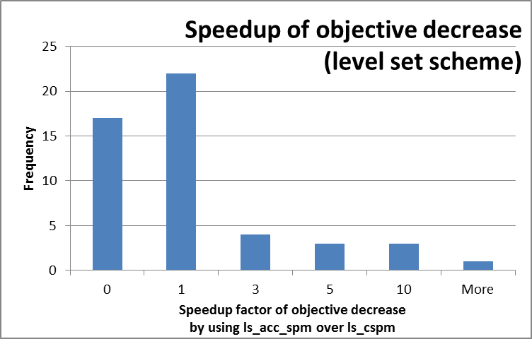
(a) Level set scheme

(b) Bisection scheme

Figure 3. Factor of how much the objective function decreased faster in the accelerated versions of the schemes (QPS problems). A speedup factor of 0 means that no difference in speed was observed. Negative speedups indicate that the indicated scheme performed worse over the compared method.

For the bisection scheme and QPS problems, there is no difference in the rate of objective decrease between accelerated and basic version. Therefore, for certain problem types, the accelerated level set scheme using CSPM has a great potential to speed up the rate of objective decrease and only causes a very moderate increase in the number of projections required by the algorithm (only about 1.5 times as many for 17 problems).

4.4. Are the superiorized versions a good choice for the level set scheme?

The quality scores in Tables 2 and 3 seem to indicate that the superiorized version outperform their basic variants in both schemes. However, for the QPS problems, the t-tests for paired two sample mean comparisons showed that there is, in fact, no statistically significant difference in the means (p-values for two-tailed tests were 0.148 for the level set scheme comparison between ls_acc_cspm and ls_acc_sup_cspm and 0.292 for the bisection scheme comparison between bis_art3+ and bis_sup_art3+). Nevertheless, for our test cases, the superiorized versions in the level set scheme outperformed their basic counterparts in more cases: the superiorized version ls_sup_acc_cspm produced a quality score at least as good as the basic version ls_acc_cspm in about 68% of all cases, in 64% it could actually get a better score.

On the other hand, for the IMRT problems, the superiorized versions clearly outperform the basic versions in terms of objective function scores. Statistical tests are all significant up to a level of 0.0013 (p-value for two-tailed tests of test for mean difference being 0). This clearly shows a promising feature of superiorized algorithms: they are very often able to obtain better solutions, even when used in an optimization framework. The accelerated versions of the superiorized schemes, however, did not differ in quality from their unaccelerated versions.

However, the superiorized versions require more projections and objective evaluations than the normal versions (see Figures 4 and 5). In these charts, the horizontal axis again denotes the multiplication factor by which the number of projections or objective function evaluations of the basic versions would have to be multiplied to be equal to the values for the superiorized versions. An increase factor of 0 means that the indicated scheme needed as many projections as the compared method. In many instances, the superiorized versions required more than 10 times the number of projections over the basic variant, leading to significantly higher computation times.

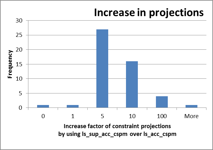
(a) Increase in projections

(b) Increase in objective evaluations

Figure 4. Factor of how much the complexity increases by using the superiorized version of CSPM in the level set scheme (QPS problems).

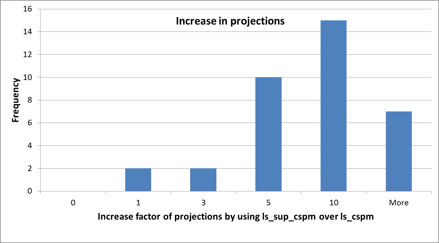
(a) Increase in projections

(b) Increase in objective evaluations

Figure 5. Factor of how much the complexity increases by using the superiorized version of CSPM in the level set scheme (IMRT problems).

Yet, for the QPS problems, there is also some potential when it comes to the rate of decrease of the objective function, as shown in Figure 6.

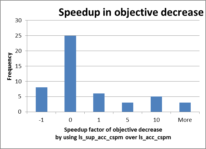
Figure 6. Factor of speedup of the objective function decrease by using the superiorized version of CSPM in the level set scheme for QPS problems. A factor of 0 indicates no difference, negative factors indicate that the superiorized version exhibited a slower decrease.

For IMRT problems, this decrease was only marginal: the rate of decrease of the superiorized versions is on average only about 0.5 times faster than the basic versions (note that 0 times would indicate they progress at the same rate).

Hence, the superiorized version of CSPM uses many more projections and evaluations. However, if these are cheap to compute, then the potential increase in objective function reduction in early iterations could lead to a faster approach overall for some problems if the user is willing to stop the optimization prematurely for practical reasons.

4.5. Which is the better optimization scheme?

We compare the level set scheme using the accelerated CSPM and the bisection scheme with CSPM, as these are the most promising candidates for each optimization scheme given the analysis above. For the QPS problems, there is no statistically significant difference in the objective score between the two methods (the p-value of the two-tailed test is 0.389). However, ls_acc_cspm outperforms the bisection scheme significantly for IMRT problems - even if 4 outliers of the 36 problems were removed (those which skewed the average quality score of the bisection scheme to the right). With a p-value of 0.007, ls_acc_cspm produces a better quality score than the equivalent bisection scheme.

Moreover, as Figure 7 shows for QPS problems, on average, the bisection scheme requires many more projections and objective evaluations. An intuitive explanation to the results is perhaps because in the bisection scheme one may be in an infeasible detecting stage several times, and in each such a stage many calculations are done (which eventually lead one to conclude that infeasibility has been detected). In the level-set scheme an infeasibility stage can happen only one time, and in the other stages usually feasibility is detected.

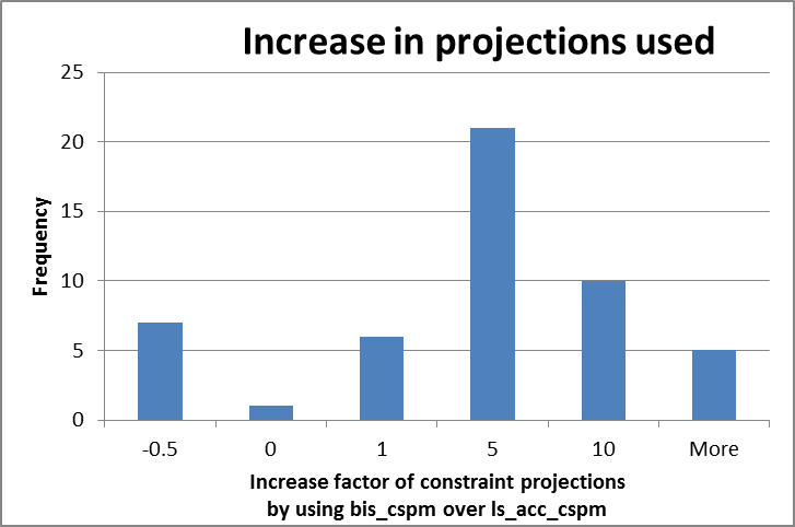
(a) Increase in projections

(b) Increase in objective evaluations

Figure 7. Factor of how much the complexity increases for QPS problems by using the bisection scheme over the level set scheme. ‘0’ indicates no difference, and negative values indicate a decrease in complexity.

For IMRT problems, the increase is less pronounced, but consistent. There the increase is up to factor 4.

In terms of rate of objective decrease, the results are mixed. In fact, it seems that bisection can be expected to decrease the objective a little faster than the level set scheme. However, Figure 8 shows that for the QPS problems this does not happen very often.

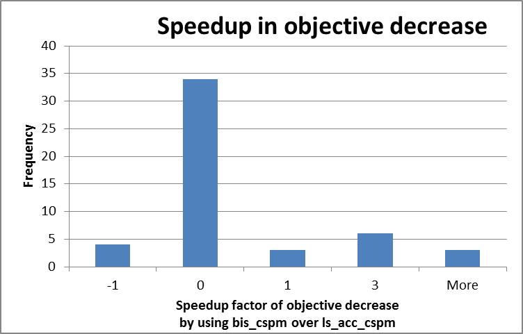
Figure 8. Factor of speedup of the objective function decrease by using the bisection scheme over the level set scheme (QPS problems).

For IMRT problems, the results are similar, however, it seems as if a speedup of factor 2 occurred quite frequently.

The level set scheme seems to be the better optimization tool for IMRT problems in terms of the quality and complexity. But, if one allows superiorization, then this is not always the case and the differences might be very minor, compare for example ”ls_sup_cspm” and ”bis_sup_cspmsee” in Tables 2 and 3. Overall, although both strategies are able to obtain similar qualities in the solutions for the QPS problems, there is a clear advantage of the level set scheme over the bisection scheme when it comes to complexity.

5. Concluding remarks and Further research

Projection methods are known for their computational efficiency and simplicity. This is the reason we decided to use a well-known reformulation of a convex optimization problem and apply projection methods within that general scheme. While at this point the convergence proof for the scheme is valid only when finite convergent algorithms are used, numerical experiments show that general convergent algorithms also generate good solutions when the stopping rule is chosen in an educated way. We believe that the mathematical validity of this relies on Remark 4.1 and is still under investigation.

Another direction we plan to investigate is based on Yamagishi and Yamada results [75], which show how to replace the subgradient projections by a more efficient projection when additional knowledge, such as lower bounds is provided. In addition we plan to study accelerating techniques for projection methods, for example the recent work of Pang [68] and [69]. Another direction for investigation is the usage of other type of projection methods, for example Bregman projection, see e.g., [33].

References

- [1] S. Agmon, The relaxation method for linear inequalities, Canadian Journal of Mathematics 6 (1954), 382–392.
- [2] D. Amelunxen, Geometric analysis of the condition of the convex feasibility problem, Ph. D. Dissertation, University of Paderborn, 2011.
- [3] H. H. Bauschke and J. M. Borwein, On projection algorithms for solving convex feasibility problems, SIAM Review 38 (1996), 367–426.
- [4] H. H. Bauschke and P. L. Combettes, Convex Analysis and Monotone Operator Theory in Hilbert Spaces, Springer Science+Business Media, LLC, Second Edition 2017.
- [5] H. H. Bauschke and V. R. Koch, Projection Methods: Swiss Army Knives for Solving Feasibility and Best Approximation Problems with Halfspaces, Contemporary Mathematics 636 (2015), 1–40.
- [6] M. S. Bazaraa, H. D. Sherali and C. M. Shetty, Nonlinear Programming: Theory and Algorithms: 3nd edition, John Wiley & Sons Inc, Hoboken, New-Jersey, USA, 2006.
- [7] R. Gordon, R. Bender and G. T. Herman, Algebraic reconstruction techniques (ART) for three-dimensional electron microscopy and x-ray photography, Journal of Theoretical Biology 29 (1970), 471–481.
- [8] D. P. Bertsekas, Nonlinear Programming: 2nd Edition, Athena Scientific, Belmont, Massachusetts, USA 1999.
- [9] D. Blatt and A. O. Hero, III: Energy based sensor network source localization via projection onto convex sets (POCS). IEEE Transactions on Signal Processing 54 (2006), 3614–-3619.
- [10] S. P. Boyd and L. Vandenberghe, Convex Optimization, Cambridge University Press, Cambridge, 2004.
- [11] S. Boyd and L. Vandenberghe, Localization and Cutting-Plane Methods, Lecture topics and notes, 2008. https://see.stanford.edu/materials/lsocoee364b/05-localization_methods_notes.pdf
- [12] S. Boyd and J. Park, Subgradient Methods, Notes for EE364b, Stanford University, 2014. https://stanford.edu/class/ee364b/lectures/subgrad_method_notes.pdf
- [13] D. Butnariu, Y. Censor, P. Gurfil and E. Hadar, On the behavior of subgradient projections methods for convex feasibility problems in Euclidean spaces, SIAM Journal on Optimization 19 (2008), 786–807.
- [14] D. Butnariu, R. Davidi, G. T. Herman and I. G. Kazantsev, Stable convergence behavior under summable perturbations of a class of projection methods for convex feasibility and optimization problems, IEEE Journal of Selected Topics in Signal Processing 1 (2007), 540–547.
- [15] C. Byrne, Iterative projection onto convex sets using multiple Bregman distances, Inverse Problems 15 (1999), 1295–1313.
- [16] C. Byrne, A unified treatment of some iterative algorithms in signal processing and image reconstruction, Inverse Problems 20 (2004), 103–120.
- [17] A. Cegielski, A method of projection onto an acute cone with level control in convex minimization, Mathematical Programming 85 (1999), 469–490.
- [18] A. Cegielski and Y. Censor, Projection methods: An annotated bibliography of books and reviews, Optimization 64 (2015), 2343–2358.
- [19] A. Cegielski and R. Dylewski, Selection strategies in a projection method for convex minimization problems, Discussiones Mathematicae. Differential Inclusions, Control and Optimization 22 (2002), 97–123.
- [20] A. Cegielski and R. Dylewski, Residual selection in a projection method for convex minimization problems, Optimization 52 (2003), 211–220.
- [21] Y. Censor, Weak and strong superiorization: Between feasibility-seeking and minimization, Analele Stiintifice ale Universitatii Ovidius Constanta-Seria Matematica 23 (2015), 41–54.
- [22] Y. Censor, Superiorization and Perturbation Resilience of Algorithms: A Bibliography compiled and continuously updated by Yair Censor, http://math.haifa.ac.il/yair/bib-superiorization-censor.html. Website last updated: 2 March 2017, arXiv version: arXiv:1506.04219 [math.OC] ([v2], 9 Mar 2017).
- [23] Y. Censor, M. D. Altschuler and W. D. Powlis, On the use of Cimmino’s simultaneous projections method for computing a solution of the inverse problem in radiation therapy treatment planning, Inverse Problems 4 (1988), 607–623.
- [24] Y. Censor, W. Chen, P. L. Combettes, R. Davidi and G. T. Herman, On the effectiveness of projection methods for convex feasibility problems with linear inequality constraints, Computational Optimization and Applications 51 (2012), 1065–1088.
- [25] Y. Censor, W. Chen and H. Pajoohesh, Finite convergence of a subgradient projections method with expanding controls, Applied Mathematics and Optimization 64 (2011), 273–285.
- [26] Y. Censor, R. Davidi and G. T. Herman, Perturbation resilience and superiorization of iterative algorithms, Inverse Problems 26 (2010), 065008 (12pp).
- [27] Y. Censor, T. Elfving, N. Kopf and T. Bortfeld, The multiple-sets split feasibility problem and its applications for inverse problems, Inverse Problems 21 (2005), 2071–2084.
- [28] Y. Censor, G. T. Herman, and M. Jiang (Guest Editors). Special issue on Superiorization: Theory and Applications, Inverse Problems 33 (2017).
- [29] Y. Censor and A. Lent, Cyclic subgradient projections, Mathematics Publication Series, Report No 35. Department of Mathematics, University of Haifa, 1981.
- [30] Y. Censor and A. Lent, Cyclic subgradient projections, Mathematical Programming 24 (1982), 233–235.
- [31] Y. Censor and D. Reem, Zero-convex functions, perturbation resilience, and subgradient projections for feasibility-seeking methods, Mathematical Programming, (Ser. A) 152 (2015), 339–380.
- [32] Y. Censor and E. Tom, Convergence of string-averaging projection schemes for inconsistent convex feasibility problems, Optimization Methods and Software 18 (2003), 543–554.
- [33] Y. Censor and S. A. Zenios, Parallel Optimization: Theory, Algorithms and Applications, Oxford University Press, New York, NY, USA, 1997.
- [34] Y. Censor and S. A. Zenios, Interval-constrained matrix balancing, Linear Algebra and Its Applications 150 (1991), 393–421.
- [35] Y. Censor and Y. Zur, Linear superiorization for infeasible linear programming, in: Y. Kochetov, M. Khachay, V. Beresnev, E. Nurminski and P. Pardalos (Editors), Discrete Optimization and Operations Research, Lecture Notes in Computer Science (LNCS), Vol. 9869, (2016), Springer International Publishing, pp. 15–24.
- [36] A. E. Cetin, H. Ozaktas and H. M. Ozaktas, Resolution enhancement of low resolution wavefields with POCS algorithm. Electronics Letters 39 (2003), 1808–-1810.
- [37] G. Cimmino, Calcolo approssimato per le soluzioni dei sistemi di equazioni lineari, La Ricerca Scientifica (Roma) 1 (1938), 326–333.
- [38] W. Chen, D. Craft, T. M. Madden, K. Zhang, H. M. Kooy and G. T. Herman, A fast optimization algorithm for multi-criteria intensity modulated proton therapy planning, Medical Physics 37 (2010), 4938–4945.
- [39] J. W. Chinneck, Feasibility and Infeasibility in Optimization: Algorithms and Computational Methods, International Series in Operations Research & Management Science 118 ,Springer-Verlag, US, 2008.
- [40] CoinUtils package availble from https://projects.coin-or.org/CoinUtils. Last updated 22.04.2013.
- [41] P. L. Combettes and J. Luo, An adaptive level set method for nondifferentiable constrained image recovery, IEEE Transactions on Image Processing 11 (2002), 1295–1304.
- [42] A. R. De Pierro and A. N. Iusem, A finitely convergent “row-action” method for the convex feasibility problem, Applied Mathematics and Optimization 17 (1988), 225–235.
- [43] A. R. De Pierro and E. S. Helou Neto, From convex feasibility to convex constrained optimization using block action projection methods and underrelaxation, International Transactions in Operational Research 16 (2009), 495–504.
- [44] J. Elzinga and T. G. Moore, A central cutting plane algorithm for the convex programming problem, Mathematical Programming Studies, 8 (1975), 134–145.
- [45] M. Fukushima, A finitely convergent algorithm for convex inequalities, IEEE Transactions on Automatic Control 27 (1982), 1126–1127.
- [46] L. G. Gubin, B.T . Polyak and E. V. Raik, The method of projections for finding a common point of convex sets, Computational Mathematics and Mathematical Physics 7 (1967), 1–24.
- [47] J.-L. Goffin and K. C. Kiwiel, Convergence of a simple subgradient level method, Mathematical Programming 85 (1999), 207–211.
- [48] J.-L. Goffin, Z.-Q. Luo and Y. Ye, Complexity analysis of an interior cutting plane method for convex feasibility problems, SIAM Journal on Optimization 6 (1996), 638–652.
- [49] G. T. Herman, Superiorization for image analysis, in: Combinatorial Image Analysis, Lecture Notes in Computer Science 8466, Springer, 2014, 1–7.
- [50] G. T. Herman and W. Chen, A fast algorithm for solving a linear feasibility problem with application to intensity-modulated radiation therapy, Linear Algebra and Its Applications 428 (2008), 1207–1217.
- [51] G. T. Herman, E. Garduňo, R. Davidi and Y. Censor, Superiorization: An optimization heuristic for medical physics, Medical Physics 39 (2012), 5532–5546.
- [52] G. T. Herman and L. Meyer, Algebraic reconstruction techniques can be made computationally efficient, IEEE Transactions on Medical Imaging 12 (1993), 600–609.
- [53] J.-B. Hiriart-Urruty and C. Lemaréchal, Fundamentals of Convex Analysis, Springer-Verlag, Berlin, Heidelberg, Germany, 2001.
- [54] A. N. Iusem and L. Moledo, On finitely convergent iterative methods for the convex feasibility problem, Bulletin of the Brazilian Mathematical Society 18 (1987), 11–18.
- [55] S. Kaczmarz, Angenöherte Auflösung von Systemen linearer Gleichungen, Bulletin de l’Académie Polonaise des Sciences at Lettres A35 (1937), 355–357.
- [56] J. E. Kelley, The cutting-plane method for solving convex programs, Journal of the Society for Industrial and Applied Mathematics 8 (1960), 703–712.
- [57] R. F. Khabibullin, On a method to find a point of a convex set, Journal of Soviet Mathematics 39 (1987), 2958–2963. Translated from Issledovaniya po Prikladnoi Matematike 4 (1977), 23–30.
- [58] R. F. Khabibullin, Generalized descent method for minimization of functionals, Journal of Soviet Mathematics 39 (1987), 2963–2968. Translated from Issledovaniya po Prikladnoi Matematike 4 (1977), 23–30.
- [59] S. Kim, H. Ahn and S.-C. Cho, Variable target value subgradient method, Mathematical Programming 49 (1990), 359–369
- [60] K. C. Kiwiel, The efficiency of subgradient projection methods for convex optimization, Part I: General level methods and Part II: Implementations and extensions, SIAM Journal on Control and Optimization 34 (1996), 660–697.
- [61] I. V. Konnov, A combined relaxation method for variational inequalities with nonlinear constraints, Mathematical Programming 80 (1998), 239–252.
- [62] K.-H. Küfer, M. Monz A. Scherrer, P. Süss, F. V. Alonso, A. S. Azizi Sultan, T. Bortfeld and C. Thieke, Multicriteria optimization in intensity modulated radiotherapy planning, in: Handbook of Optimization in Medicine (Springer Optimization and Its Applications) 26 (2009), 123–167.
- [63] A. N. Kulikov and V. R. Fazylov, A finite method to find a point in a set defined by a convex differentiable functional, Journal of Soviet Mathematics 45 (1989), 1273–1277.
- [64] C. Lemaréchal, A. Nemirovskii and Y. Nesterov, New variants of bundle methods, Mathematical Programming 69 (1995), 111—-147.
- [65] I. Maros and Cs. Mészáros, A Repository of Convex Quadratic Programming Problems, Optimization Methods and Software 11 (1999), 671–681.
- [66] D. Q. Mayne, E. Polak and A. J. Heunis, Solving nonlinear inequalities in a finite number of iterations, Journal of Optimization Theory and Applications 33 (1981), 207–221.
- [67] T. S. Motzkin and I. J. Schoenberg, The relaxation method for linear inequalities, Canadian Journal of Mathematics 6 (1954), 393–404.
- [68] C. H. J. Pang, Set intersection problems: Supporting hyperplanes and quadratic programming, Mathematical Programming (Ser. A) 149 (2015), 329–359.
- [69] C. H. J. Pang, SHDQP: An algorithm for convex set intersection problems based on supporting hyperplanes and dual quadratic programming, arXiv:1307.0053 [math.OC], (2013; current version: [v3], 15 Feb 2015)
- [70] E. Polak and D. Q. Mayne, On the finite solution of nonlinear inequalities, IEEE Transactions on Automatic Control 24 (1979), 443–445.
- [71] D. Reem and A. De Pierro, A new convergence analysis and perturbation resilience of some accelerated proximal forward-backward algorithms with errors, Inverse Problems 33 (2017) 044001 (28pp), arXiv:1508.05631 [math.OC], 2015 (current version: [v3], 29 Jun 2016)
- [72] A. Scherrer, F. Yaneva, T. Grebe and K.-H. Küfer, A new mathematical approach for handling DVH criteria in IMRT planning, Journal of Global Optimization 61 (2015), 407–428.
- [73] J. van Tiel, Convex Analysis: An Introductory Text, John Wiley and Sons, Universities Press, Belfast, Northern Ireland, 1984
- [74] B. J. van Wyk and M. A. van Wyk, A POCS-based graph matching algorithm. IEEE Transactions on Pattern Analysis and Machine Intelligence 26 (2004), 1526-–1530.
- [75] M. Yamagishi and I. Yamada, A Deep Monotone Approximation Operator Based on the Best Quadratic Lower Bound of Convex Functions, IEICE Transactions on Fundamentals of Electronics, Communications and Computer Sciences E91-A (2008), 1858–1866.
- [76] S. A. Zenios and Y. Censor, Massively parallel row-action algorithms for some nonlinear transportation problems, SIAM Journal on Optimization 1 (1991), 373–400.