Tuning a random field mechanism in a frustrated magnet

Abstract

We study the influence of spinless impurities on a frustrated magnet featuring a spin-density wave (stripe) phase by means of Monte Carlo simulations. We demonstrate that the interplay between the impurities and an order parameter that breaks a real-space symmetry triggers the emergence of a random-field mechanism which destroys the stripe-ordered phase. Importantly, the strength of the emerging random fields can be tuned by the repulsion between the impurity atoms; they vanish for perfect anticorrelations between neighboring impurities. This provides a novel way of controlling the phase diagram of a many-particle system. In addition, we also investigate the effects of the impurities on the character of the phase transitions between the stripe-ordered, ferromagnetic, and paramagnetic phases.

Introduction:

Low-temperature phases of many-particle systems usually break one or several of the symmetries of the interactions spontaneously. This is well described by the concept of order parameters (OPs), quantities that vanish in the symmetric phase but are nonzero (and nonunique) in the symmetry-broken phase (see, e.g., Ref. Goldenfeld ). A simple example of an OP is the total magnetization which measures the degree to which the spin rotation symmetry is broken. In recent years, lots of attention has been attracted by phases that spontaneously break real-space symmetries in addition to spin, phase, or gauge symmetries, for example by rendering the $x$ and $y$ directions in a crystal inequivalent. Such phases include the charge-density wave or stripe phases in cuprate superconductors, the Ising-nematic phases in the iron pnictides fradkin ; fernandes ; fkt15 , valence-bond-solids in quantum magnets mlpm06 ; sandvik07 ; sen_sandvik10 and the crystalline phases of certain lattice-gas models of hard-core particles rdd15 .

Realistic materials always contain some quenched disorder or randomness in the form of vacancies, impurity atoms, random strains, and other types of imperfections. Consequently, the question of how such randomness affects different broken symmetries and thus different OPs is crucial for understanding the materials’ behaviors (for recent reviews see, e.g., Refs. Vojta06 ; Vojta13 ).

In this Letter, we focus on the impact of random disorder on a phase that breaks a real space symmetry. To do so we turn our attention to a frustrated Ising model on a square lattice having ferromagnetic nearest-neighbor interactions and antiferromagnetic next-nearest-neighbor interactions. The disorder takes the form of spinless impurities or vacancies that dilute the magnetic lattice. The resulting Hamiltonian reads

$$H=-J_{1}\sum_{\langle ij\rangle}\rho_{i}\rho_{j}S_{i}S_{j}-J_{2}\sum_{\langle\langle ij\rangle\rangle}\rho_{i}\rho_{j}S_{i}S_{j}$$ (1)

where the $S_{i}=\pm 1$ are classical Ising variables, while $J_{1}>0$ and $J_{2}<0$ are the nearest-neighbor and next-nearest-neighbor interactions, respectively. The $\rho_{i}$ are quenched random variables that take the values 0 (vacancy) with probability $p$ and $1$ (site occupied by spin) with probability $1-p$. We consider both uncorrelated randomness for which the $\rho_{i}$ are statistically independent and anticorrelated randomness for which repulsion between the impurities suppresses the simultaneous occupation of two nearest-neighbor sites by impurities.

In the absence of vacancies ($p=0$), the phase diagram and the phase transitions of this system are well-understood (see, e.g., Refs. arnab1 ; arnab2 ; kalz ; kalzprb2012 and references therein). At high temperatures, it features a conventional paramagnetic phase. Upon lowering the temperature, two distinct symmetry-broken phases appear. For $g=|\rm{J_{2}}|/\rm{J_{1}}<1/2$, the system enters a ferromagnetic (FM) low-temperature phase that breaks the $Z_{2}$ Ising symmetry but none of the real-space symmetries. For $g>1/2$, in contrast, the low-temperature phase displays a stripe-like spin order that breaks not only the Ising symmetry but also the $Z_{4}$ rotation symmetry of the square lattice. The Hamiltonian (1) is thus particulary well suited for our study as it allows us to contrast an OP that does not break any real-space symmetries with one that does.

To analyze how the site dilution influences the frustrated Ising model (1), we perform extensive Monte Carlo simulations. We also determine the exact ground states of small plaquettes to understand the disorder effects microscopically. Our results are illustrated by the phase diagram shown in Fig. 1 and can be summarized as follows.

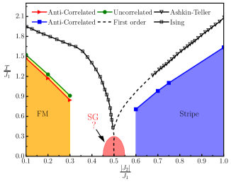
Figure 1: Phase diagram of $\rm{J_{1}}$-$\rm{J_{2}}$ Hamiltonian (1) for both uncorrelated and anti-correlated site dilution at an impurity concentration of $p=1/8$ compared to the phase diagram of the undiluted system (open symbols) kalz ; kalzprb2012 . For uncorrelated impurities, the emergent random field mechanism destroys the stripe-ordered phase. In contrast, this phase survives the introduction of anti-correlated disorder.

The ferromagnetic low-temperature phase survives moderate dilution with both uncorrelated and anticorrelated impurities, but its Curie temperature $T_{c}$ is suppressed. In contrast, the stripe-ordered low-temperature phase is completely absent for uncorrelated impurities. This is caused by an effective random field for the stripe order that emerges due to the interplay of the impurities and the broken real-space symmetry. This emergent random field destroys the stripe order via domain formation imryma ; fernandez . Importantly, the strength of the random fields can be controlled by the repulsion between the impurities; it completely vanishes if the repulsion prohibits the simultaneous occupation of nearest-neighbor sites by impurities. In this case of perfect local anticorrelations between the impurities, the stripe-ordered low-temperature phase survives, albeit with a depressed critical temperature $T_{c}$ compared to the undiluted system. This tunable random-field mechanism is the main result of this Letter. In addition, we demonstrate that the first-order phase transitions of the undiluted system are rounded by the disorder, in line with the Aizenmann-Wehr theorem aizenmann ; berker . In the rest of this Letter, we discuss our simulations, explain the tunable random-field mechanism, and put our results into a broader perspective.

Monte Carlo simulations:

We employ standard single-spin flip Metropolis MRRT53 simulations of the Hamiltonian (1). We study square lattices of linear sizes between $L=8$ to 80, averaging the results over 500 to 1000 disorder configurations. Details of the simulation algorithm and parameter values can be found in the Supplemental Material Supplemental . The primary observables are the OPs for the ferromagnetic and stripe phases. The two-component stripe OP $\psi\equiv(\psi_{x},\psi_{y})$ is defined as arnab1 ; arnab2

$$\psi_{x}=\frac{1}{L^{2}}\sum_{i}\rho_{i}S_{i}(-1)^{x_{i}},\quad\psi_{y}=\frac{1}{L^{2}}\sum_{i=1}\rho_{i}S_{i}(-1)^{y_{i}},$$ (2)

where $(x_{i},y_{i})$ are the coordinates of site $i$ whereas the ferromagnetic OP, i.e., the magnetization, reads

$$m=\frac{1}{L^{2}}\sum_{i}\rho_{i}S_{i}~{}.$$ (3)

We also analyze the corresponding susceptibilities $\chi_{S}=L^{2}\left[\langle\psi^{2}\rangle-\langle|\psi|\rangle^{2}\right]/T$ and $\chi_{F}=L^{2}\left[\langle m^{2}\rangle-\langle|m|\rangle^{2}\right]/T$ as well as the Binder cumulants

$$U_{\rm S}=2\left(1-\frac{1}{2}\frac{\left[\langle\psi^{4}\rangle\right]}{{\left[\langle\psi^{2}\rangle\right]}^{2}}\right),~{}U_{\rm F}=\frac{3}{2}\left(1-\frac{1}{3}\frac{\left[\langle m^{4}\rangle\right]}{{\left[\langle m^{2}\rangle\right]}^{2}}\right)~{}.$$ (4)

Here, $\left[\cdots\right]$ denotes the average over disorder realizations whereas $\langle\cdots\rangle$ indicates the usual thermodynamic (Monte Carlo) average. The Binder cumulants are normalized such that they take the limiting values $U_{\rm F,S}\rightarrow 1$ deep in the corresponding ordered phases and $U_{\rm F,S}\rightarrow 0$ deep in the disordered phase. The crossing of the Binder cumulant curves for different system sizes yields the location of the phase transition. The Binder cumulant also allows us to determine the order of the transition: For a continuous transition, it is a monotonic function of temperature binder . At a first-order transition, in contrast, the Binder cumulant shows a minimum that becomes more pronounced with increasing system size vollmayr and is caused by the existence of multiple peaks in the OP distribution. This non-monotonic temperature dependence can serve as an indicator of a first-order transition.

Stripe Phase:

We now turn to the central question of this Letter, the fate of the stripe phase upon introducing spinless impurities. Figure 2 depicts the stripe OP and the associated susceptibility for dilution $p=1/4$, contrasting the cases of uncorrelated impurities and perfectly anticorrelated impurities (where the simultaneous occupation of nearest-neighbor sites by impurities is forbidden). The frustration parameter is $g=|J_{2}|/J_{1}=1$ for which the undiluted system features a stripe-ordered low-temperature phase.

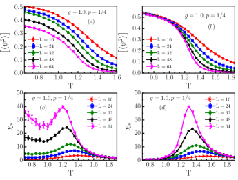
Figure 2: Stripe order-parameter $\psi$ and stripe susceptibility $\chi_{S}$ as functions of temperature $T$ for frustration parameter $g=1$, dilution $p=1/4$ and several system sizes. Data for uncorrelated vacancies are shown in panels (a) and (c) whereas panels (b) and (d) show results for anti-correlated vacancies.

Figure 2(a) shows that the stripe order-parameter at low temperatures decreases with increasing system size for the case of uncorrelated impurities. In this case, the stripe susceptibility shown in Fig. 2(c) develops a pronounced secondary peak at low temperatures. As suggested in Ref. fernandez , these observations indicate the absence of long-range stripe order in the thermodynamic limit. In contrast, in the case of anticorrelated disorder, the stripe order-parameter saturates at a size-independent nonzero value at low temperatures, as shown in Fig. 2(b). The corresponding stripe susceptibility, shown in Fig. 2(d), displays the conventional behavior associated with a continuous phase transition. These observations suggest that the stripe order survives in the case of anticorrelated impurities.

To provide further evidence, we compare the behavior of the stripe Binder cumulants $U_{\rm S}(T)$ for uncorrelated and anticorrelated impurities. Figure 3 depicts the Binder cumulants for the same parameters used above, viz., $p=1/4$ and $g=1$.

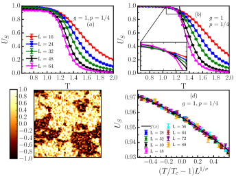
Figure 3: Stripe Binder cumulant $U_{S}$ vs. temperature $T$ for frustration parameter $g=1$, dilution $p=1/4$ and several system sizes. Panel (a) shows data for uncorrelated impurities whereas results for anticorrelated impurities are presented in panel (b). Panel (c): Local nematic OP $\eta_{i}$ for a single system of 100x100 sites, uncorrelated impurities with dilution $p=1/4$, $T=0.55$, and $g=1$. Panel (d) shows the scaling collapse (with $\bar{\chi}^{2}=0.97$) of the stripe Binder cumulant for anticorrelated impurities and $g=1$, $p=1/4$.

Focussing on Fig. 3(a), we see that for uncorrelated impurities, the Binder cumulant vs. temperature curves for different system sizes do not cross. With increasing size, the Binder cumulant shifts to smaller and smaller values, i.e., towards the disordered phase, confirming the absence of long-range stripe order for the case of uncorrelated impurities. The fate of the stripe phase can be further illustrated via the nematic OP $\eta=\psi_{x}^{2}-\psi_{y}^{2}$ which measures the local preference for vertical vs. horizontal stripes. The color plot in Fig. 3(c) shows the local nematic OP for each $2\times 2$ plaquette, clearly demonstrating competing domains of horizontal and vertical stripes Supplemental .

In contrast, for the case of anticorrelated impurities, the stripe Binder cumulants for different system sizes do cross as evidenced in Fig. 3(b). This indicates the existence of a phase transitions and thus the survival of the stripe-ordered low-temperature phase. Estimates of the transition temperature $T_{c}$ and the correlation length exponent $\nu$ can be obtained from finite-size scaling Barber_review83 ; Cardy_book88 (for details, see Supplemental material Supplemental ). Figure 3(d) shows the scaling collapse of the Binder cumulant in terms of the scaled variable $(T-T_{c})L^{1/\nu}$, with $T_{c}=1.1729(5)$ and $\nu=1.26(3)$. The data collapse is very good; the underlying least-square fit has a reduced $\bar{\chi}^{2}=0.97$ note1 . Because our systems are only moderately large, the value of $\nu$ should be understood as an effective exponent rather than the true asymptotic exponent.

Random fields from spinless impurities:

To explain the absence of the stripe phase for uncorrelated impurities, we now demonstrate that the impurities induce effective random fields for the nematic OP $\eta=\psi_{x}^{2}-\psi_{y}^{2}$. We focus on the ground state energies of small plaquettes of $2\times 2$ sites as seen in Fig. 4.

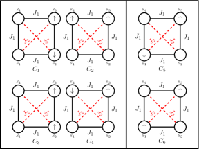
Figure 4: Impurity configurations on $2\times 2$ plaquettes illustrating the emergence of random-field disorder for the stripe OP (see text for further details).

If impurities simultaneously occupy two vertical nearest-neighbor sites (configurations $C_{1}$ and $C_{3}$ in Fig. 4), vertical stripes (configuration $C_{3}$) are favored over horizontal stripes (configuration $C_{1}$) as their ground state energy on the plaquette is lower by $-2J_{1}$. Analogously, if impurities occupy two horizontal nearest-neighbor sites (configurations $C_{2}$ and $C_{4}$), horizontal stripes ($C_{2}$) are favored over vertical stripes ($C_{4}$). In contrast, configurations with either a single impurity or two impurities across the diagonal of a plaquette ($C_{5}$ and $C_{6}$) do not prefer one stripe orientation over the other.

This means that impurity configurations in which two impurities occupy nearest neighbor sites locally break the $Z_{4}$ lattice rotation symmetry. They thus act as random fields for the nematic OP $\eta$ by locally preferring either the $\psi_{x}$ or the $\psi_{y}$ component of the stripe OP (2). As was argued by Imry and Ma imryma in the context of the random-field Ising model nattermann1 and later proven rigorously aizenmann , random fields destroy the long-range ordered phase via domain formation. Monte Carlo evidence for domains was presented in Fig. 3(c).

The typical size $L_{D}$ of these domains depends on the strength of the random fields and thus on the dilution $p$. In two dimensions, the dependence is expected to be exponential, $L_{D}\sim\exp\left({\rm const}/p^{4}\right)$, for small $p$ nattermann1 . This implies that the domain size will exceed the system size for sufficiently small $p$, making the destruction of the long-range order unobservable Supplemental .

The fact that a local preference for vertical or horizontal stripes only appears if two impurities occupy two nearest-neighbor sites can be used to tune the strength of the emerging random field mechanism. If the probability for nearest-neighbor pairs of impurities is reduced, for example because of a repulsive interaction between the impurities, fewer random fields appear in the system. In the limit of perfectly anticorrelated impurities where such pairs are completely forbidden, the random-field mechanism is switched off note2 . This explains why our simulations showed that the stripe-ordered phase survives for anticorrelated impurities.

Ferromagnetic phase:

In contrast to the stripe OP, the total magnetization does not break a real-space symmetry. Therefore, spinless impurities do not create random fields coupling to the ferromagnetic order. Instead, they act as much more benign random-mass or random-$T_{c}$ disorder. Consequently, the ferromagnetic phase survives in the presence of impurities, be they uncorrelated or perfectly anticorrelated. However, the Curie temperature $T_{c}$ is reduced compared to the undiluted system, as is shown in the phase diagram in Fig. 1.

Phase transitions:

We now turn to the phase transitions between the paramagnetic, ferromagnetic, and stripe phases. The transitions of the undiluted system are well understood arnab1 ; arnab2 ; kalz ; kalzprb2012 . As illustrated in Fig. 1, there is a direct first-order phase transition between the ferromagnetic and stripe phases at low temperatures. The transition between the ferromagnetic and paramagnetic phases is continuous and belongs to the 2D Ising universality class. Extensive numerical simulations have also established that the transition from the stripe phase to the paramagnetic phase is of first order for $g<g^{*}\approx 0.67$. The line of first-order transition terminates at $g^{*}$ and gives rise to critical behavior that belongs to the Ashkin-Teller universality class AToriginal .

In the presence of anticorrelated disorder, the ferromagnetic and stripe phases both survive. According to Landau Landau , phase transitions between two ordered phases that break different symmetries must be of first order. However, the Aizenman-Wehr theorem aizenmann forbids first-order transitions in two-dimensional disordered systems. This implies that the ferromagnetic and stripe phases must be separated by an intermediate phase. This could simply be the paramagnetic phase extending all the way to zero temperature, or there could be a spin glass (SG) phase at low temperatures and $g$ close to 0.5. Unequivocally resolving the phases in this parameter region is beyond the scope of this Letter.

The stripe to paramagnetic transition of the undiluted system is of first-order for $0.5<g<g^{*}\approx 0.67$. To determine the character of this transition in the presence of anticorrelated impurities, we analyze the stripe Binder cumulant $U_{S}$ in Fig. 5.

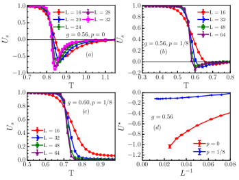
Figure 5: Stripe Binder cumulant $U_{S}$ vs. temperature for different system sizes. (a) undiluted system, $p=0$, $g=0.56$; (b) anticorrelated impurities, $p=1/8$, $g=0.56$; (c) anticorrelated impurities, $p=1/8$, $g=0.60$; (d) minimum value $U^{*}$ as a function of inverse system size.

In the undiluted system depicted in Fig. 5(a), $U_{S}$ shows a pronounced minimum close to the transition which gets deeper with system size (see also Fig. 5(d)). This clearly indicates a first-order transition. In contrast, in the diluted system with $p=1/8$ and $g=0.6$ shown in Fig. 5(c), $U_{S}$ does not feature any minima, demonstrating that the first-order transition is rounded to a continuous one, in agreement with the Aizenman-Wehr theorem aizenmann . For the diluted system at $g=0.56$, the Binder cumulant shows weak minima, but they do not deepen with system size. This can be attributed to the fact that the clean first-order transition is stronger at smaller $g$. The disorder-induced rounding will therefore occur at a larger length scale beyond the moderate sizes used in our simulations. This is compatible with the size dependence shown in Fig. 5(d).

The ferromagnetic to paramagnetic transition survives for both uncorrelated and anticorrelated impurities. The critical behavior across all phase transition lines in the diluted case is compatible with the two-dimensional Ising universality class with logarithmic corrections, as is discussed in the Supplemental Material Supplemental .

Conclusions:

In summary, we have studied the effects of spinless impurities on the phases of a frustrated Ising magnet. As the impurities do not break the Ising symmetry of the ferromagnetic OP, they act as rather benign random-mass disorder in the ferromagnetic phase. Consequently, this phase survives in the presence of the impurities, albeit with reduced Curie temperature. In contrast, the impurities can locally break the symmetry between horizontal and vertical stripes and thus create effective random fields for the nematic OP. These emerging random fields destroy the stripe phase via domain formation.

The microscopic understanding of the random fields has allowed us to identify a way to tune their strength. The random fields are suppressed with increasing repulsion between the impurities and completely vanish if nearest-neighbor pairs of impurities are forbidden. Therefore, the stripe phase survives for such perfectly anticorrelated impurities. This mechanism offers a novel way of controlling the phase diagram of a many-particle system. Note that the protection of the stripe phase by local (anti-)correlations between the impurities is similar to the protection of a clean quantum critical point by local disorder correlations discussed in Ref. joselaflorencieetal .

Finally, we comment on the possibility of a nematic phase in the Hamiltonian (1). In principle, the paramagnetic to stripe phase transition could split into two separate transitions: The $Z_{4}$ lattice symmetry is broken first, leading to nematic order, while the Ising spin symmetry is broken at a lower temperature. Nematic order has indeed been observed in a $J_{1}$-$J_{2}$ model in an external field alejandra . However, our simulations have not provided any indications of a nematic phase in our problem.

Acknowledgements:

A.S. is partly supported through the Partner Group program between the Indian Association for the Cultivation of Science (IACS), Kolkata and the Max Planck Institute for the Physics of Complex Systems (MPIPKS), Dresden. T.V. is supported in part by the NSF under Grants No. PHY-1125915 and No. DMR- 1506152. The numerical data were generated at the PG Senapathy computing facility at Indian Institute of Technology, Madras, the computing facility at the Department of Theoretical Physics, IACS and the computing facility at MPIPKS.

Supplemental material for:
Tuning a random field mechanism in a frustrated magnet

Shashikant Singh Kunwar¹, Arnab Sen², Thomas Vojta³, and Rajesh Narayanan¹

¹ Department of Physics, Indian Institute of Technology Madras, Chennai 600036, India.
² Department of Theoretical Physics, Indian Association for the Cultivation of Science, Jadavpur, Kolkata 700032, India.
³ Department of Physics, Missouri University of Science and Technology, Rolla, Missouri 65409, USA.

S1. Details of Monte-Carlo procedure

We employ the classical single-spin-flip Metropolis algorithm S_MRRT53 to perform our simulations because cluster-flip methods such as the Swendsen-Wang S_SwendsenWang87 and Wolff S_Wolff89 algorithms do not improve the performance in the presence of frustrated interactions. We study square lattices of linear size $L=8$ to 80. Each Monte Carlo simulation consists of an equilibration period of $10^{6}$ Monte Carlo sweeps (a sweep corresponds to one attempted spin flip per lattice site), followed by a measurement period of another $10^{6}$ sweeps, with measurements taken after each sweep. To improve the equilibration performance, we adopt a cooling procedure. We start the simulations at high temperatures and lower the temperature in small steps, using the final state of the higher temperature simulation as the initial condition for the next lower temperature.

We investigate frustration parameters $g=|J_{2}|/J_{1}$ between 0.1 and 1.0. To study the influence of disorder, a total number of $N_{imp}=pL^{2}$ spinless impurity sites are introduced into the lattice. These impurities are either completely uncorrelated or they are perfectly anticorrelated such that the simultaneous occupation of nearest-neighbor sites by impurities is forbidden. We simulate dilutions of $p=1/8$ and 1/4. We expect, however, that the qualitative results hold for all values of $p$ that are sufficiently small such that lattice percolation effects do not play a role. All observables are averaged over $1000$ impurity configurations for the smaller system sizes, $L=8$ to $32$, and over 500 impurity configurations for the larger sizes.

S2. Finite-size scaling analysis

In this section we describe the methodology adopted to extract the critical temperature $T_{c}$ and the critical exponents from the Monte Carlo data of the site-diluted ${J_{1}}$-${J_{2}}$ model. The analysis is based on finite-size scaling S_Barber_review83 ; S_Cardy_book88 of the stripe and ferromagnetic Binder cumulants $U_{S}$ and $U_{F}$ as well as the corresponding susceptibilities $\chi_{S}$ and $\chi_{F}$.

S2.1 Ferromagnetic transition

We start by analyzing the ferromagnetic Binder cumulant $U_{\rm F}$ defined as

$$U_{\rm F}=\frac{3}{2}\left(1-\frac{1}{3}\frac{\left[\langle m^{4}\rangle\right]}{{\left[\langle m^{2}\rangle\right]}^{2}}\right)~{}.$$ (S1)

According to finite-size scaling, the Binder cumulant values for different system sizes $L$ and temperatures $T$ should collapse onto a single master curve when plotted as a function of the scaling variable $x=(T-T_{c})L^{1/\nu}$ where $\nu$ is the correlation length critical exponent. Moreover, as the Binder cumulant is a dimensionless quantity, its value right at $T_{c}$ should be size-independent, implying a Taylor expansion

$$U_{\rm F,S}(T,L)=f(x)=a_{0}+a_{1}x+a_{2}x^{2}+\ldots.$$ (S2)

sufficiently close to the critical point. Figures S1(a) and (b) show examples of such scaling plots for uncorrelated impurities at concentration $p=1/8$ and frustration parameters $g=0$ and 0.3, respectively.

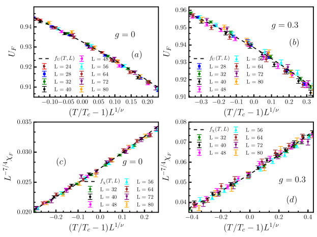
Figure S1: Scaling collapse of the ferromagnetic binder cumulant $U_{F}$ [panels (a) and (b)] and the scaled ferromagnetic susceptibility $\chi_{F}L^{-7/4}$ [panels (c) and (d)] for uncorrelated impurities at $p=1/8$ and frustration parameters $g=0$ and 0.3.

The values of $T_{c}$ and $\nu$ are extracted from fits of the $U_{F}$ data to the expansion (S2) truncated after the quadratic term. The quality of the fit can be estimated from the reduced sum of squared errors (per degree of freedom) $\bar{\chi}^{2}$ defined as

$$\bar{\chi}^{2}=\frac{1}{N-M}\sum_{i=1}^{N}\frac{[U_{F,i}-f(x_{i})]^{2}}{\sigma_{i}^{2}}~{}.$$ (S3)

Here, $N$ is the number of data points, $M$ is the number of fit-parameters, and $\sigma_{i}^{2}$ is the (Monte Carlo) variance of the value $U_{F,i}$. The fits are considered of good quality when $\bar{\chi}^{2}\lessapprox 1$. Results of this analysis for both uncorrelated and anticorrelated impurities and several values of the frustration parameter $g$ are presented in Table 1.

	anticorrelated			uncorrelated
$g$	$T_{c}$	$\nu$	$\bar{\chi}^{2}$	$T_{c}$	$\nu$	$\bar{\chi}^{2}$
$0$	$1.7574(1)$	$1.16(1)$	$1.19$	$1.8036(1)$	$1.12(1)$	$1.36$
$0.1$	$1.4724(1)$	$1.11(1)$	$0.71$	$1.5234(1)$	$1.13(2)$	$1.37$
$0.2$	$1.1728(1)$	$1.14(3)$	$1.01$	$1.2294(1)$	$1.17(2)$	$1.10$
$0.3$	$0.8450(2)$	$1.14(4)$	$0.82$	$0.9108(2)$	$1.15(4)$	$1.45$

Table 1: Critical temperatures $T_{c}$, effective correlation length exponents $\nu$, and reduced error sums $\bar{\chi}^{2}$ obtained from the scaling analysis of the ferromagnetic Binder cumulant $U_{F}$. Results are shown for various values of the frustration parameter $g$ and dilution $p=1/8$ for both uncorrelated and anticorrelated impurities. The numbers in parentheses give the error of the last digit.

How do our results for the correlation length exponent $\nu$ compare to theoretical predictions? The ferromagnetic-to-paramagnetic transition in the clean, undiluted system belongs to the two-dimensional Ising universality class. Its correlation length exponent takes the value $\nu_{cl}=1$ implying that random-mass disorder is exactly marginal according to the Harris criterion $d\nu>2$ S_harris . The fate of the phase transition in the two-dimensional disordered Ising model has been controversially discussed in the literature (see, e.g., Ref. S_qiong and references therein). Recent numerical results S_qiong demonstrate, however, that the critical behavior of the disordered Ising model is controlled by the clean two-dimensional Ising critical point but with universal logarithmic corrections as predicted by perturbative renormalization group calculations. Our system sizes are too small to reliably extract logarithmic corrections. The $\nu$ values in Table 1 must therefore be considered effective rather than asymptotic exponent values. They are comparable to effective $\nu$ values found in the above-mentioned high-precision study of the disordered Ising model. We thus conclude that our results are consistent with the critical behavior of the ferromagnetic transition belonging to the disordered Ising universality class.

Further evidence is provided by the ferromagnetic susceptibility $\chi_{F}$. Anticipating two-dimensional Ising critical behavior for which the susceptibility has a scale dimension of 7/4, we analyze the scaling collapse of $L^{-7/4}\chi_{F}$ S_note3 . Figures S1(c) and (d) show the scaling plots of the susceptibility data for uncorrelated impurities at concentration $p=1/8$ and frustration parameters $g=0$ and 0.3, respectively. As in the case of the Binder cumulants, the data collapse is of good quality. Values for $T_{c}$ and $\nu$ can be found by fitting the susceptibility to the expansion

$$L^{-7/4}\chi_{\rm F,S}(T,L)=f(x)=a_{0}+a_{1}x+a_{2}x^{2}+\ldots.$$ (S4)

The resulting values are summarized in Table 2.

	anticorrelated			uncorrelated
$g$	$T_{c}$	$\nu$	$\bar{\chi}^{2}$	$T_{c}$	$\nu$	$\bar{\chi}^{2}$
$0$	$1.7573(2)$	$1.14(3)$	$0.64$	$1.8031(2)$	$1.10(2)$	$0.80$
$0.1$	$1.4719(2)$	$1.10(2)$	$1.05$	$1.5234(3)$	$1.13(4)$	$0.97$
$0.2$	$1.1720(2)$	$1.12(3)$	$0.96$	$1.2287(2)$	$1.22(4)$	$0.72$
$0.3$	$0.8440(4)$	$1.04(6)$	$0.77$	$0.9102(3)$	$1.18(4)$	$1.21$

Table 2: Critical temperatures $T_{c}$, effective correlation length exponents $\nu$, and reduced error sums $\bar{\chi}^{2}$ obtained from the scaling analysis of the ferromagnetic susceptibility $\chi_{F}$. Results are shown for various values of the frustration parameter $g$ and dilution $p=1/8$ for both uncorrelated and anticorrelated impurities.

They agree well with those from the analysis of the Binder cumulant. (For the effective exponent $\nu$, the deviations are within one standard deviation; for $T_{c}$ they are within two standard deviations.)

S2.2 Stripe transition

The stripe-ordered to paramagnetic transition can be analyzed along the same lines as the ferromagnetic transition above. Because uncorrelated impurities completely destroy the stripe phase, we only consider perfectly anticorrelated impurities. Figure S2 presents example scaling plots of the stripe Binder cumulant $U_{S}$ and the stripe susceptibility $\chi_{S}$ for impurity concentration $p=1/8$ and frustration parameters $g=0.75$ and $g=1$.

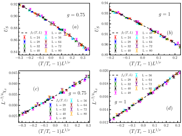
Figure S2: Scaling plots of the stripe cumulant $U_{S}$ [panels (a) and (b)] and the stripe susceptibility $\chi_{S}$ [panels (c) and (d)] for anticorrelated impurities of concentration of $p=1/8$ and frustration parameters $g=0.75$ and $g=1$.

The values of $T_{c}$ and the correlation length exponent $\nu$ can again be determined from fits to Eqs. (S2) and (S4). The results are summarized in Table 3.

	Binder cumulant $U_{S}$			susceptibility $\chi_{S}$
$g$	$T_{c}$	$\nu$	$\bar{\chi}^{2}$	$T_{c}$	$\nu$	$\bar{\chi}^{2}$
$0.60$	$0.70766(9)$	$0.93(2)$	$0.92$
$0.70$	$0.9827(1)$	$0.99(3)$	$1.10$	$0.9838(1)$	$1.04(2)$	$1.57$
$0.75$	$1.1020(1)$	$1.00(2)$	$1.09$	$1.1029(1)$	$1.04(2)$	$1.34$
$1$	$1.6361(1)$	$1.05(2)$	$1.09$	$1.6362(1)$	$1.07(1)$	$1.01$

Table 3: Critical temperatures $T_{c}$, effective correlation length exponents $\nu$, and reduced error sums $\bar{\chi}^{2}$ obtained from the scaling analysis of the stripe Binder cumulant $U_{S}$ and the stripe susceptibility $\chi_{S}$. Results are shown for various values of the frustration parameter $g$ and dilution $p=1/8$ for perfectly anticorrelated impurities.

In the undiluted, clean system, the stripe to paramagnetic transition is either of first-order (for $g<g^{*}\approx 0.67$) or belongs to the Ashkin-Teller universality class (for $g>g^{*}$) kalz ; kalzprb2012 ; arnab1 ; arnab2 ). We have shown in the main text that the first-order transition is rounded to a continuous one in the presence of anticorrelated impurities, as is expected from the Aizenman-Wehr theorem S_aizenmann . Our results in Table 3 show that the critical exponent $\nu$ of the diluted system is close to the clean Ising value of unity for all studied values of $g$. In particular, $\nu$ does not vary systematically with $g$ as would be expected for the clean Ashkin-Teller universality class. The effects of disorder on the Ashkin-Teller universality class were studied by Murthy S_Murthy and Cardy S_Cardy via a renormalization group analysis that predicted clean Ising critical behavior with universal logarithmic corrections just as in the disordered Ising model. This was recently confirmed by large-scale simulations S_qiong . As in the case of the ferromagnetic transition above, the system sizes in our present work are too small to extract logarithmic corrections. However, the effective $\nu$ values in Table 3 are close to the clean two-dimensional Ising value of unity. We conclude that our results are consistent with the critical behavior of the stripe transition belonging the disordered Ising universality class.

S3. Domains

As discussed in the main text, spinless impurities in the $J_{1}$-$J_{2}$ Hamiltonian create random fields for the nematic order parameter $\eta=\psi_{x}^{2}-\psi_{y}^{2}$ which measures the local preference for vertical vs. horizontal stripes. These random fields destroy the long-range stripe order via domain formation. In order to image these domains, we define a local version of the nematic order parameter via $\eta_{i}=(\bar{\psi}_{i,x}^{2}-\bar{\psi}_{i,y}^{2})$ where $\bar{\psi}_{i,x}$ and $\bar{\psi}_{i,y}$ are formed by averaging $\psi_{i,x}=S_{i}(-1)^{x_{i}}$, and $\psi_{i,y}=S_{i}(-1)^{y_{i}}$ over $2\times 2$ plaquette number $i$.

Figure S3 illustrates the emergence of the domains in a system of linear size $L=100$ at $g=1$ and $T=0.55$ as we increase the concentration $p$ of impurities. For impurity concentration $p=1/8$, the local order parameter fluctuates only slightly, i.e., the entire system belongs to a single domain. For the more disordered sample, $p=1/4$, the characteristic domain size has fallen below the system size. The figure now shows random-field induced domain walls percolating throughout the sample, thus leading to the destruction of long-range stripe order.

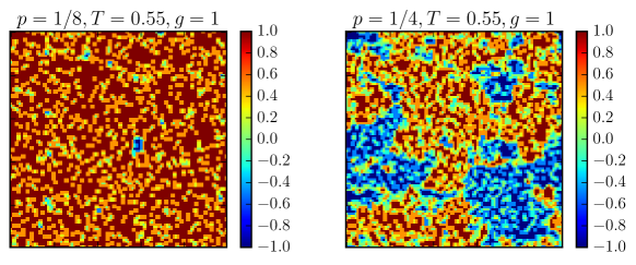
Figure S3: Local nematic order parameter $\eta_{i}$ for each $2\times 2$ plaquette of a single system of 100x100 sites for $T=0.55$, $g=1$, and uncorrelated impurities of concentration $p=1/8$ (left panel) and $p=1/4$ (right panel).

References

- (1) N. Goldenfeld, Lectures on Phase transitions and the Renormalization Group (Addison-Wesley, Reading, MA, 1992).
- (2) E. Fradkin, S. A. Kivelson, M. J. Lawler, J. P. Eisenstein, and A. P. Mackenzie, Annu. Rev. Condens. Matter Phys. 1,153 (2010).
- (3) R. M. Fernandes, A. V. Chubukov and J. Schmalian, Nat. Phys. 10, 97 (2014).
- (4) E. Fradkin, S. A. Kivelson, and J. M. Tranquada, Rev. Mod. Phys. 87, 457 (2015).
- (5) M. Mambrini, A. Läuchli, D. Poilblanc, and F. Mila, Phys. Rev. B 74, 144422 (2006).
- (6) A. W. Sandvik, Phys. Rev. Lett. 98, 227202 (2007).
- (7) A. Sen and A. W. Sandvik, Phys. Rev. B 82, 174428 (2010).
- (8) K. Ramola, K. Damle, and D. Dhar, Phys. Rev. Lett. 114, 190601 (2015).
- (9) T.Vojta, J. Phys. A 39, R143 (2006).
- (10) T. Vojta, AIP Conference Proceedings 1550, 188 (2013).
- (11) A. Kalz, A. Honecker, and M. Moliner, Phys. Rev. B 84, 174407 (2011).
- (12) A. Kalz and A. Honecker, Phys. Rev. B 86, 134410 (2012).
- (13) S. Jin, A. Sen, A.W. Sandvik, Phys. Rev. Lett. 108, 045702 (2012).
- (14) S. Jin, A. Sen, W. Guo, A.W. Sandvik, Phys. Rev. B 87, 144406 (2013).
- (15) Y. Imry and S.K. Ma, Phys. Rev. Lett. 35, 1399 (1975).
- (16) J. F. Fernandez EPL 5, 129 (1988).
- (17) M. Aizenman and J. Wehr, Phys. Rev. Lett. 62, 2503 (1989).
- (18) K. Hui and A. N. Berker, Phys. Rev. Lett. 62, 2507 (1985); A. N. Berker, Physica A 194, 72 (1993).
- (19) K. Binder, Phys. Rev. Lett. 47, 693 (1981).
- (20) K. Vollmayr, J. D. Reger, M. Scheucher, and K. Binder, Z. Phys. B 91, 113 (1993).
- (21) N. Metropolis, A. Rosenbluth, M. Rosenbluth and A. Teller, J. Chem. Phys. 21, 1087 (1953).
- (22) See Supplemental Material at XXX with references SwendsenWang87 to Cardy for details of the Monte Carlo algorithm, the scaling analysis of the ferromagnetic and stripe phase transitions, as well as the domain formation.
- (23) R. H. Swendsen and J.-S. Wang, Phys. Rev. Lett. 58, 86 (1987).
- (24) U. Wolff, Phys. Rev. Lett. 62, 361 (1989).
- (25) A. B. Harris, J. Phys. C 7, 1671 (1974).
- (26) Qiong Zhu, Xin Wan, Rajesh Narayanan, Jose A. Hoyos, Thomas Vojta, Phys. Rev. B 91, 224201 (2015).
- (27) N. Murthy, Phys. Rev. B 36, 7166 (1987).
- (28) J. Cardy, J. Phys. A 29, 1897 (1996); Physica A 263, 215 (1999).
- (29) M. N. Barber, in Phase Transitions and Critical Phenomena, edited by C. Domb and J. L. Lebowitz (Academic, New York, 1983), Vol. 8. pp. 145.
- (30) J. Cardy (Ed), Finite-size scaling (North Holland, Amsterdam, 1988).
- (31) T. Nattermann, in Spin Glasses and Random Fields, edited by A.P. Young (World Scientific, Singapore, 1997).
- (32) M. Schwartz, J. Villain, Y. Shapir and T. Nattermann, Phys. Rev B 48, 3095 (1993).
- (33) L. D. Landau, Zh. Eksp. Teor. Fiz. 7, 19 (1937). [Phys. Z. Sowjetunion 11, 26 (1937)]; Zh. Eksp. Teor. Fiz. 7, 627 (1937). [Phys. Z. Sowjetunion 11, 545 (1937)].
- (34) J. Ashkin and E. Teller, Phys. Rev. 64, 178 (1943); C. Fan and F. Y. Wu, Phys. Rev. B 2, 723 (1970); L. P. Kadanoff and F. J. Wegner, Phys. Rev. B 4, 3989 (1971).
- (35) J. A. Hoyos, N. Laflorencie, A. P. Vieira, T. Vojta, Europhys. Lett. 93, 30004 (2011)
- (36) Alejandra I. Guerrero, Daniel A. Stariolo, and Noé G. Almarza, Phys. Rev. E, 91, 052123 (2015).
- (37) We denote the reduced sum of squared errors of the fit (per degree of freedom) by to distinguish it from the susceptibility .
- (38) Strictly, this arguments holds at only. At finite temperatures, random fields may be generated via entropic effects nattermann . However, at low temperatures they are expected to be extremely weak and likely unobservable in experiments and simulations.

References

- (1) N. Metropolis, A. Rosenbluth, M. Rosenbluth and A. Teller, J. Chem. Phys. 21, 1087 (1953).
- (2) R. H. Swendsen and J.-S. Wang, Phys. Rev. Lett. 58, 86 (1987).
- (3) U. Wolff, Phys. Rev. Lett. 62, 361 (1989).
- (4) M. N. Barber, in Phase Transitions and Critical Phenomena, edited by C. Domb and J. L. Lebowitz (Academic, New York, 1983), Vol. 8. pp. 145.
- (5) J. Cardy (Ed), Finite-size scaling (North Holland, Amsterdam, 1988).
- (6) A. B. Harris, J. Phys. C 7, 1671 (1974).
- (7) Qiong Zhu, Xin Wan, Rajesh Narayanan, Jose A. Hoyos, Thomas Vojta, Phys. Rev. B 91, 224201 (2015).
- (8) A. Kalz, A. Honecker, and M. Moliner, Phys. Rev. B 84, 174407 (2011).
- (9) A. Kalz and A. Honecker, Phys. Rev. B 86, 134410 (2012).
- (10) S. Jin, A. Sen, A.W. Sandvik, Phys. Rev. Lett. 108, 045702 (2012).
- (11) S. Jin, A. Sen, W. Guo, A.W. Sandvik, Phys. Rev. B 87, 144406 (2013).
- (12) M. Aizenman and J. Wehr, Phys. Rev. Lett. 62, 2503 (1989).
- (13) N. Murthy, Phys. Rev. B 36, 7166 (1987).
- (14) J. Cardy, J. Phys. A 29, 1897 (1996); Physica A 263, 215 (1999).
- (15) As for the Binder cumulant, logarithmic corrections to the clean Ising behavior are expected. Our system sizes are too small, however, to reliably extract these logarithms.