The Penetration Effect of Connected Automated Vehicles in Urban Traffic: An Energy Impact Study

Abstract

Earlier work has established a decentralized framework of optimally controlling connected and automated vehicles (CAVs) crossing an urban intersection without using explicit traffic signaling. The proposed solution is capable of minimizing energy consumption subject to a throughput maximization requirement. In this paper, we address the problem of optimally controlling CAVs under mixed traffic conditions where both CAVs and human-driven vehicles (non-CAVs) travel on the roads, so as to minimize energy consumption while guaranteeing safety constraints. The impact of CAVs on overall energy consumption is also investigated under different traffic scenarios. The benefit from CAV penetration (i.e., the fraction of CAVs relative to all vehicles) is validated through simulation in MATLAB and VISSIM. The results indicate that the energy efficiency improvement becomes more significant as the CAV penetration rate increases, while the significance diminishes as the traffic becomes heavier.

I Introduction

To date, traffic light signaling is the prevailing method used for controlling the traffic flow at urban intersections. Exploiting data-driven control and optimization approaches, recent research (e.g., see [1]) has enabled the adaptive adjustment of traffic light cycles, leading to reduced congestion. However, aside from the obvious infrastructure cost, urban traffic lights can lead to more rear-end collisions and reduced safety. These issues have motivated research efforts on new approaches for signal-free intersection traffic control.

Connected and Automated Vehicles (CAVs) possess the potential to change the transportation landscape by enabling users to better monitor transportation network conditions and to improve traffic flow in terms of reducing energy consumption, travel delays, accidents and greenhouse gas emissions. One of the very early efforts was proposed in [2], where an optimal linear feedback regulator is designed to control a string of vehicles. Dresner and Stone [3] proposed a reservation-based scheme for automated vehicle intersection management, whereby a centralized controller coordinates the vehicle crossing sequence based on the request received from the vehicles. Numerous efforts based on reservation schemes have been reported in the literature [4, 5, 6]. Reducing the travel delay and increasing the throughput of an intersection is one desired goal to be achieved. Relevant efforts include [7, 8, 9, 10] which aim at minimizing the vehicle travel time under collision-avoidance constraints. Lee and Park [11] focused on minimizing the overlap between vehicle positions. Miculescu and Karaman [12] used a polling-system to model the intersection. A detailed discussion of the research in the literature can be found in [13].

Our earlier work [14] has established a decentralized optimal control framework for coordinating online a continuous flow of CAVs crossing an urban intersection without using explicit traffic signaling. For each CAV, an energy minimization optimal control problem is formulated where the time to cross the intersection is first determined through a throughput maximization problem. We also established conditions under which feasible solutions to the optimal control problem exist.

The benefits of CAV coordination and control on energy consumption have been established and quantified in recent literature [15, 16, 17, 18]. However, the integration of CAVs with conventional vehicles faces several challenges before their penetration rate (i.e., the fraction of CAVs relative to all vehicles in a transportation system) becomes significant. Thus, a critical question is that of determining the penetration effect of CAVs under mixed traffic conditions. Under such conditions, it is necessary to design control algorithms for CAVs and coordination policies that can accommodate both CAVs and conventional human-driven vehicles. Dresner and Stone [19] proposed a light model that can control the physical traffic lights as well as implementing a reservation-based control algorithm for autonomous vehicles while ensuring safety. Other efforts include using information from CAVs to better adapt the traffic light in a mixed traffic scenario (e.g., see [20]). In this paper, we address the problem of optimally controlling the CAVs crossing an urban intersection in a mixed traffic scenario where both CAVs and non-CAVs (conventional human-driven vehicles) travel on the roads. A decentralized optimal control framework is presented whose solution yields the optimal acceleration/deceleration so as to minimize the energy consumption subject to a throughput maximizing requirement, while taking the interaction between CAVs and non-CAVs into consideration.

The structure of the paper is as follows. In Section II, we review the model in [14] and its generalization in [21]. In Section III, we formulate the optimal control problem for each CAV under mixed traffic conditions and present the analytical solutions. In Section IV, we introduce the non-CAV model and the approaches for collision avoidance among CAVs and non-CAVs to complete the establishment of the mixed traffic scenario. In Section V, we investigate the impact of CAV penetration on energy economy under different traffic scenarios. We offer concluding remarks in Section VI.

II The Model

We briefly review the model introduced in [14] where there are two intersections, 1 and 2, located within a distance $D$ (Fig. 1). The region at the center of each intersection, called Merging Zone (MZ), is the area of potential lateral CAV collision. Although it is not restrictive, this is taken to be a square of side $S$. Each intersection has a Control Zone (CZ) and a coordinator that can communicate with the CAVs traveling within it. The distance between the entry of the CZ and the entry of the MZ is $L>S$, and it is assumed to be the same for all entry points to a given CZ.

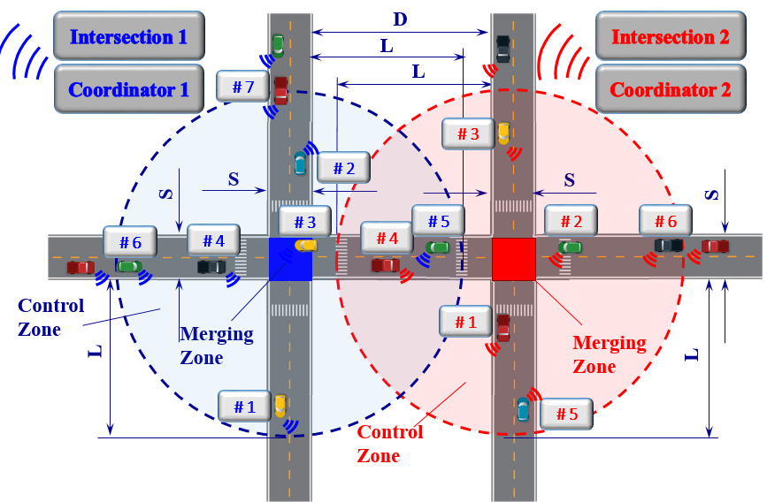
Figure 1: Connected Automated Vehicles (CAVs) crossing two adjacent intersections.

Let $N_{z}(t)\in\mathbb{N}$ be the cumulative number of CAVs which have entered the CZ of intersection $z$ at $t$ and formed a queue $\mathcal{N}_{z}(t)=\{1,\ldots,N_{z}(t)\}$ which designates the order in which these vehicles will be entering the MZ. The way the queue is formed is not restrictive. When a CAV reaches the CZ of intersection $z$, the coordinator assigns it an integer value $i=N_{z}(t)+1$. If two or more CAVs enter a CZ at the same time, then the corresponding coordinator selects randomly the first one to be assigned the value $N_{z}(t)+1$. In the region between the exit point of a MZ and the entry point of the subsequent CZ, the CAVs are assumed to cruise with the speed they had when they exited that MZ.

For simplicity, we assume that each CAV is governed by second order dynamics:

$$\dot{p}_{i}(t)=v_{i}(t)\text{, }~{}p_{i}(t_{i}^{0})=0\text{; }~{}\dot{v}_{i}(t)=u_{i}(t)\text{, }v_{i}(t_{i}^{0})\text{ given}$$ (1)

where $p_{i}(t)$, $v_{i}(t)$, and $u_{i}(t)$ denote the position (i.e., travel distance since the entry of the CZ), speed and acceleration/deceleration (i.e., control input) of each CAV $i$. These dynamics are in force over an interval $[t_{i}^{0},t_{i}^{f}]$, where $t_{i}^{0}$ and $t_{i}^{f}$ are the times that CAV $i$ enters the CZ and exits the MZ of intersection $z$ respectively.

To ensure that the control input and vehicle speed are within a given admissible range, the following constraints are imposed:

$$\begin{split}u_{i,min}&\leq u_{i}(t)\leq u_{i,max},\quad\text{and}\\ 0&\leq v_{min}\leq v_{i}(t)\leq v_{max},\quad\forall t\in[t_{i}^{0},t_{i}^{m}],\end{split}$$ (2)

where $t_{i}^{m}$ is the time that CAV $i$ enters the MZ.

Definition 1

Depending on its physical location inside the CZ, CAV $j\in\mathcal{N}_{z}(t),j\neq i$ belongs to only one of the following four subsets of $\mathcal{N}_{z}(t)$ with respect to CAV $i$: 1) $\mathcal{R}^{z}_{i}(t)$ contains all CAVs traveling on the same road as $i$ and towards the same direction but on different lanes, 2) $\mathcal{L}^{z}_{i}(t)$ contains all CAVs traveling on the same road and lane as vehicle $i$ (e.g., $\mathcal{L}^{1}_{6}(t)$ contains CAV #4 in Fig. 1), 3) $\mathcal{C}^{z}_{i}(t)$ contains all CAVs traveling on different roads from $i$ and having destinations that can cause collision at the MZ (e.g., $\mathcal{C}^{1}_{7}(t)$ contains CAV #6 in Fig. 1), and 4) $\mathcal{O}^{z}_{i}(t)$ contains all CAVs traveling on the same road as $i$ and opposite destinations that cannot, however, cause collision at the MZ (e.g., $\mathcal{O}^{1}_{4}(t)$ contains CAV #3 in Fig. 1).

To ensure the absence of any rear-end collision throughout the CZ, we impose the rear-end safety constraint:

$$s_{i}(t)=p_{k}(t)-p_{i}(t)\geq\delta,~{}\forall t\in[t_{i}^{0},t_{i}^{m}],~{}k\in\mathcal{L}_{i}^{z}(t)$$ (3)

where $k$ is the CAV physically ahead of $i$ on the same lane, $s_{i}(t)$ is the inter-vehicle distance between $i$ and $k$, and $\delta$ is the minimal safety following distance allowable.

A lateral collision involving CAV $i$ may occur only if some CAV $j\neq i$ belongs to $\mathcal{C}^{z}_{i}(t)$. This leads to the following definition:

Definition 2

For each CAV $i\in\mathcal{N}_{z}(t)$, we define the set $\Gamma_{i}$ that includes all time instants when a lateral collision involving CAV $i$ is possible: $\Gamma_{i}\triangleq\Big{\{}t~{}|~{}t\in[t_{i}^{m},t_{i}^{f}]\Big{\}}$.

Consequently, to avoid a lateral collision for any two vehicles $i,j\in\mathcal{N}_{z}(t)$ on different roads, the following constraint should hold

$$\Gamma_{i}\cap\Gamma_{j}=\varnothing,\text{ \ }\forall t\in[t_{i}^{m},t_{i}^{f}]\text{, \ }j\in\mathcal{C}^{z}_{i}(t).$$ (4)

As part of safety considerations, we impose the following assumption (which may be relaxed if necessary):

Assumption 1

For CAV $i$, none of the constraints in (2)-(3) is active at $t_{i}^{0}$.

Assumption 2

The speed of the CAVs inside the MZ is constant, i.e., $v_{i}(t)=v_{i}(t_{i}^{m})=v_{i}(t_{i}^{f})$, $\forall t\in[t_{i}^{m},t_{i}^{f}]$. This implies that $t_{i}^{f}=t_{i}^{m}+\frac{S}{v_{i}(t_{i}^{m})}$.

Assumption 3

Each CAV $i$ has proximity sensors and can measure local information without errors or delays.

The objective of each CAV is to derive an optimal acceleration/deceleration profile, in terms of minimizing energy consumption, inside the CZ (i.e., over the time interval $[t_{i}^{0},t_{i}^{m}]$) while avoiding congestion between the two intersections. Since the coordinator is not involved in any decision making process on the vehicle control, we can formulate $N_{1}(t)$ and $N_{2}(t)$ decentralized tractable problems for intersection 1 and 2 respectively that can be solved online. The terminal times for CAVs entering the MZ can be obtained as the solutions to a throughput maximization problem formulated in [21] subject to rear-end and lateral collision avoidance constraints inside the MZ. As shown in [21], the terminal time of CAV $i$ (i.e., $t_{i}^{m}$) can be recursively determined through

$$t_{i}^{m^{\ast}}=\left\{\begin{array}[c]{ll}t_{1}^{m^{\ast}}&\mbox{if $i=1$}\\ \text{max }\{t_{i-1}^{m^{\ast}},t_{k}^{m^{\ast}}+\frac{\delta}{v_{k}^{m}},t_{i}^{c}\}&\text{if }i-1\in\mathcal{R}^{z}_{i}\cup\mathcal{O}^{z}_{i}\\ \text{max }\{t_{i-1}^{m^{\ast}}+\frac{\delta}{v_{i-1}^{m}},t_{i}^{c}\}&\mbox{if $i-1\in\mathcal{L}^{z}_{i}$}\\ \text{max }\{t_{i-1}^{m^{\ast}}+\frac{S}{v_{i-1}^{m}},t_{i}^{c}\}&\mbox{if $i-1\in\mathcal{C}^{z}_{i}$}\end{array}\right.$$ (5)

where $t_{i}^{c}=t_{i}^{1}\mathds{1}_{v_{i}^{m}=v_{max}}+t_{i}^{2}(1-\mathds{1}_{v_{i}^{m}=v_{max}})$ and

$$t_{i}^{1} =t_{i}^{0}+\frac{L}{v_{max}}+\frac{(v_{max}-v_{i}^{0})^{2}}{2u_{i,max}v_{max}},$$

$$t_{i}^{2} =t_{i}^{0}+\frac{[2Lu_{i,max}+(v_{i}^{0})^{2}]^{1/2}-v_{i}^{0}}{u_{i,max}}.$$

Here, $t_{i}^{c}$ is a lower bound of $t_{i}^{m}$ regardless of the solution of the throughput maximization problem.

The conditions under which the rear-end safety constraint in (3) does not become active inside the CZ are provided in [22].

III Optimal Control of CAVs in Mixed Traffic

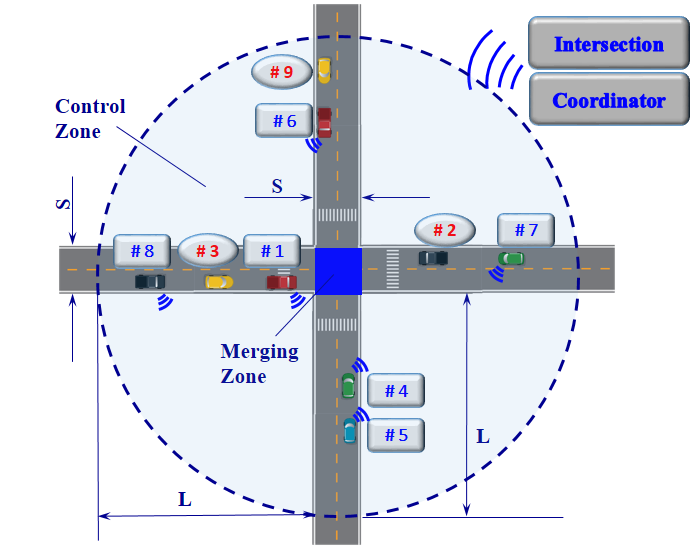
Figure 2: Connected Automated Vehicles (blue labels) and non-CAVs (red labels) crossing an urban intersection.

We consider the mixed traffic scenario (Fig. 2) where both CAVs and non-CAVs (conventional human-driven vehicles) travel on the roads. The first major issue to be addressed is modeling the interaction between CAVs and non-CAVs where we assume that the latter do not possess the capability to communicate with other vehicles.

Regarding a CAV, there are two modes that it can be in: $(i)$ Free Driving (FD mode) when it is not constrained by a non-CAV that precedes it. $(ii)$ Adaptive Following (AF mode) when it follows a preceding non-CAV while adaptively maintaining a safe following distance from it. CAVs switch from the FD mode to the AF mode as soon as the inter-vehicle distance falls below a certain threshold.

III-A Optimal Control for Free Driving (FD) Mode

In this mode, the objective of each CAV is to derive an optimal acceleration/deceleration profile, in terms of minimizing energy consumption, inside the CZ, that is,

$$\min_{u_{i}\in U_{i}}\frac{1}{2}\int_{t_{i}^{0}}^{t_{i}^{m}}K_{i}\cdot u_{i}^{2}(t)~{}dt$$

$$\text{subject to}:\eqref{eq:model2},(\ref{speed_accel constraints}),t_{i}^{m},\text{ }p_{i}(t_{i}^{0})=0\text{, }p_{i}(t_{i}^{m})=L,$$ (6)

$$\text{given }t_{i}^{0}\text{, }v_{i}(t_{i}^{0}),$$

where $K_{i}$ is a factor to capture CAV diversity (for simplicity, $K_{i}=1$ in the remainder of this paper). Note that this formulation does not include the rear-end safety constraint in the CZ in (3); we will return to this issue in what follows. On the other hand, the rear-end and lateral collision avoidance inside the MZ can be implicitly ensured by $t_{i}^{m}$.

An analytical solution of problem (6) may be obtained through a Hamiltonian analysis found in [21]. Assuming that all constraints are satisfied upon entering the CZ and that they remain inactive throughout $[t_{i}^{0},t_{i}^{m}]$, the optimal control input (acceleration/deceleration) over $t\in[t_{i}^{0},t_{i}^{m}]$ is given by

$$u_{i}^{\ast}(t)=a_{i}t+b_{i}$$ (7)

where $a_{i}$ and $b_{i}$ are constants of integration. Using (7) in the CAV dynamics (1), the optimal speed and position are obtained:

$$v_{i}^{\ast}(t)=\frac{1}{2}a_{i}t^{2}+b_{i}t+c_{i}$$ (8)

$$p_{i}^{\ast}(t)=\frac{1}{6}a_{i}t^{3}+\frac{1}{2}b_{i}t^{2}+c_{i}t+d_{i},$$ (9)

where $c_{i}$ and $d_{i}$ are constants of integration. The coefficients $a_{i}$, $b_{i}$, $c_{i}$, $d_{i}$ can be obtained given initial and terminal conditions as follows:

$$\left[\begin{array}[c]{cccc}\frac{1}{6}(t_{i}^{0})^{3}&\frac{1}{2}(t_{i}^{0})^{2}&(t_{i}^{0})&1\\ \frac{1}{2}(t_{i}^{0})^{2}&(t_{i}^{0})&1&0\\ \frac{1}{6}(t_{i}^{m})^{3}&\frac{1}{2}(t_{i}^{m})^{2}&t_{i}^{m}&1\\ -t_{i}^{m}&-1&0&0\end{array}\right].\left[\begin{array}[c]{c}a_{i}\\ b_{i}\\ c_{i}\\ d_{i}\end{array}\right]=\left[\begin{array}[c]{c}p_{i}(t_{i}^{0})\\ v_{i}(t_{i}^{0})\\ p_{i}(t_{i}^{m})\\ \lambda_{i}^{v}(t_{i}^{m})\end{array}\right]$$ (10)

Note that the analytical solution (7) is valid while none of the constraints becomes active for $t\in[t_{i}^{0},t_{i}^{m}]$. Otherwise, the optimal solution should be modified considering the constraints, as discussed in [21]. Recall that the constraint (3) is not included in (6). To address this constraint, conditions under which the CAV is able to maintain feasibility in terms of satisfying (3) over $t\in[t_{i}^{0},t_{i}^{m}]$ are derived in [22] along with an explicit mechanism to enforce them prior to entering the CZ.

III-B Optimal Control for Adaptive Following (AF) Mode

When the preceding vehicle for CAV $i$ is also a CAV, the feasibility of the optimal solution (7)-(10) can be enforced through an appropriately designed Feasibility Enforcement Zone that precedes the CZ as described in [22]. Otherwise, when the inter-vehicle distance $s_{i}(t)$ between CAV $i$ and the preceding vehicle $k$ falls below a certain threshold $\delta_{f}$ at $t_{i}^{1}$, CAV $i$ transitions from the FD to the AF mode (Fig. 3). Since CAV $i$ cannot communicate with the preceding non-CAV, it simply assumes a constant speed for the non-CAV.

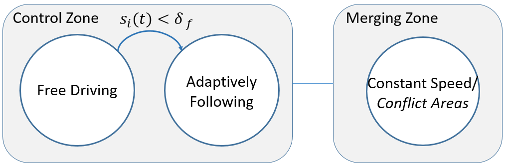
Figure 3: Modeling approach for CAVs.

In this mode, the objective of each CAV is to derive an optimal acceleration/deceleration profile so as to minimize energy consumption, while maintaining the minimum safety following distance $\delta$ with the preceding non-CAV, that is,

$$\min_{u_{i}\in U_{i}}\frac{1}{2}\int_{t_{i}^{1}}^{t_{i}^{m}}[w_{u}\cdot u_{i}^{2}(t)+w_{s}\cdot(s_{i}(t)-\delta)^{2}]~{}dt$$

$$\text{subject to}:\eqref{eq:model2},(\ref{speed_accel constraints}),t_{i}^{m},\text{ }p_{i}(t_{i}^{m})=L,$$ (11)

$$\text{and given }t_{i}^{1}\text{, }v_{i}(t_{i}^{1}),p_{i}(t_{i}^{1}),$$

where $w_{u}$ and $w_{s}$ are weights applied to the objective function, which allow trading off energy consumption minimization against maintaining the safety following distance.

The analytical solution of problem (11) may be obtained through a Hamiltonian analysis similar to that in [14] and [21]. Assuming that all constraints are satisfied at $t_{i}^{1}$ and that they remain inactive throughout $[t_{i}^{1},t_{i}^{m}]$, the optimal control input (acceleration/deceleration) over $t\in[t_{i}^{1},t_{i}^{m}]$ can be determined as follows. Defining $w=\frac{\sqrt{4w_{u}\cdot w_{s}}}{2w_{u}}$ and $\alpha=\sqrt{\frac{w}{2}}$, the optimal control can be obtained as

$$u_{i}^{*}(t) =-2a_{i}\alpha^{2}e^{\alpha t}sin(\alpha t)+2b_{i}\alpha^{2}e^{-\alpha t}sin(\alpha t)$$ (12)

$$+2c_{i}\alpha^{2}e^{\alpha t}cos(\alpha t)-2d_{i}\alpha^{2}e^{-\alpha t}cos(\alpha t).$$

The optimal speed and position can be obtained according to (1):

$$v_{i}^{*}(t) =a_{i}\cdot\alpha e^{\alpha t}(cos(\alpha t)-sin(\alpha t))$$ (13)

$$-b_{i}\cdot\alpha e^{-\alpha t}(cos(\alpha t)+sin(\alpha t))$$

$$+c_{i}\cdot\alpha e^{\alpha t}(cos(\alpha t)+sin(\alpha t))$$

$$+d_{i}\cdot\alpha e^{-\alpha t}(cos(\alpha t)-sin(\alpha t))$$

$$p_{i}^{*}(t) =a_{i}\cdot e^{\alpha t}cos(\alpha t)+b_{i}\cdot e^{-\alpha t}cos(\alpha t)$$ (14)

$$+c_{i}\cdot e^{\alpha t}sin(\alpha t)+d_{i}\cdot e^{-\alpha t}sin(\alpha t)$$

$$+p_{i-1}(t_{i}^{1})+v_{i-1}(t_{i}^{1})(t-t_{i}^{1})-\delta,$$

where $a_{i}$, $b_{i}$, $c_{i}$ and $d_{i}$ are constants of integration, which can be obtained in a similar way as (10).

III-C Terminal Conditions

Under mixed traffic conditions, the recursive terminal time structure in (5) derived in [21] can no longer be applied since non-CAVs are not controlled to follow the order imposed by the queueing structure discussed in Sec. II. To determine the terminal conditions for CAV $i$, there are two different cases to consider: $(i)$ vehicle $i-1$ is a CAV, and $(ii)$ vehicle $i-1$ is a non-CAV. If vehicle $i-1$ is a CAV, then the terminal time for CAV $i$ can be recursively determined through CAV $i-1$ as in [21]; if vehicle $i-1$ happens to be a non-CAV, then the terminal time for CAV $i$ is determined by estimating the terminal time of vehicle $i-1$. In particular, at time $t_{i}^{0}$, vehicle $i-1$ is at position $p_{i-1}(t_{i}^{0})$ with speed $v_{i-1}(t_{i}^{0})$, which can be measured by CAV $i$ through on-board sensors or through the coordinator. As CAV $i$ cannot communicate with non-CAV $i-1$, it simply assumes a constant speed for $i-1$, i.e., $v_{i-1}(t)=v_{i-1}(t_{i}^{0})$ for $t\in[t_{i}^{0},t_{i}^{m}]$. Denoting the estimated terminal time for vehicle $i-1$ as $\hat{t}_{i-1}^{m}$, we have

$$\hat{t}_{i-1}^{m} =t_{i}^{0}+\frac{L-p_{i-1}(t_{i}^{0})}{v_{i-1}(t_{i}^{0})},$$ (15)

based on which, CAV $i$ can determine its own terminal time for entering the MZ using (5). Note that the estimation may need re-evaluation in the case that non-CAV $i-1$ changes speed.

III-D Simulation Example

The proposed optimal control framework for CAVs is illustrated through the following simulation example, where the length of the CZ is $L=400$m. Vehicle #1 is assumed to be a non-CAV entering the CZ at $t_{1}^{0}=0$ and cruising at its initial speed $v_{1}^{0}=10$m/s. CAV #2 enters the same lane as vehicle #1 at $t_{2}^{0}=2$s with an initial speed $v_{2}^{0}=15$m/s. The minimum safety following distance is set to $\delta=10$m. With the weights $w_{u}$ and $w_{s}$ both set to be 1, the optimal speed trajectory of CAV #2 (i.e., $v_{2}(t)$) and the inter-vehicle distance between vehicle #1 and CAV #2 (i.e., $s_{2}(t)$) with and without the AF mode are shown in Fig. 4.

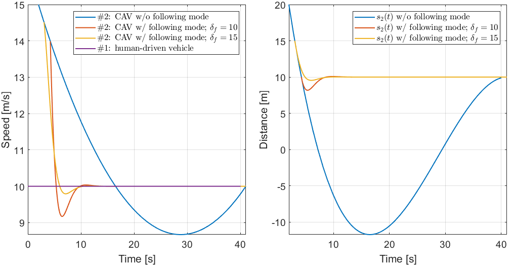
Figure 4: Speed $v_{i}(t)$ and inter-vehicle distance $s_{2}(t)$ trajectories w/ and w/o the optimal control for adaptively following.

Without a transition to the AF mode, CAV #2 violates the rear-end collision constraint (blue curve in Fig. 4) and the distance $s_{2}(t)$ falls below $\delta=10$m for $t>4.22$s. With the AF mode in force (red and yellow curves), when the distance reaches the threshold, i.e., $s_{2}(t)=\delta_{f}$, CAV #2 first decelerates so as to reach a much lower speed than vehicle #1, and then seeks to keep the distance as close to $\delta=10$m as possible. Note that the process of adaptively following implicitly forces CAV #2 to maintain the same speed as vehicle #1.

For the scenarios using the AF mode, the threshold for entering this mode is set to either $\delta_{f}=10$m (red curve) or $\delta_{f}=15$m (yellow curve). The energy consumption, given by a polynomial function of speed and acceleration, is obtained as 0.0156 and 0.0143, respectively. The energy cost reduction results from the fact that CAV #2 enters the AF mode earlier given $\delta_{f}=15$m, hence, it does not need to decelerate as hard as in the case with $\delta_{f}=10$m. The approaching process becomes smoother, which leads to lower energy consumption.

IV Modeling Methodology for non-CAVs

There are two major issues that need to be addressed in terms of modeling non-CAVs (i.e., human-driven vehicles): $(i)$ modeling the car-following behavior, and $(ii)$ designing a collision avoidance approach inside the MZ without explicit traffic signaling.

IV-A The Wiedemann Approach

In this paper, we apply the Wiedemann model [23], the default approach adopted by VISSIM, the transportation system simulator, to model car-following behavior. The basic idea of the Wiedemann model is that a non-CAV can be in one of the following four driving modes:

• Free driving: No observable influence by any preceding vehicle. In this mode, the driver seeks to reach and (approximately) maintain a desired speed.

• Approaching: The driver adapts his/her own speed to the speed of a preceding vehicle. This is done by decelerating until the speed difference becomes zero when some desired safe distance from the vehicle being followed is reached.

• Following: The driver follows the preceding vehicle while trying to (approximately) maintain a safe distance from the vehicle being followed.

• Braking: The driver applies the brake to decelerate if the distance from the preceding vehicle falls below the desired safety level. This scenario may occur if the preceding vehicle changes speed abruptly.

For each mode, there are several associated parameters that model specific car-following behavior. For instance, a “Smooth Closeup Behavior” parameter can be enabled to model less aggressive approaching behavior [23].

IV-B Conflict Areas

As non-CAVs may not follow the prescribed order in the queueing structure specified in Sec. II, lateral collisions may occur inside the MZ when no traffic lights are present. There are several ways used in VISSIM to model non-signalized intersections for non-CAVs, by defining Priority Rules, Conflict Areas, and Stop Sign Control. Among these techniques, Conflict Areas provide modeling ease and more intelligent behavior and will be adopted in the sequel to ensure the absence of lateral collisions in the MZ.

If a CAV enters the MZ at the designated terminal time $t_{i}^{m}$ while a non-CAV is present inside the MZ, the CAV simply forgoes the constant speed assumption (Assumption 2) and follows the Conflict Areas rule so as to avoid lateral collision. As shown in Fig. 5, there are three options for defining conflict areas. Fig. 5(a) indicates a passive conflict area, i.e., all vehicles are uncontrolled in terms of lateral collision avoidance (CA1). Fig. 5(b) shows a partially controlled conflict area, where the vehicles on the main road (green) are uncontrolled because they have priority to cross the MZ, while vehicles on the minor road (red) are controlled because they have to yield (CA2). Fig. 5(c) shows a fully controlled conflict area. As there is no right of way, vehicles on both roads are under control (CA3). In this paper, we use the second conflict avoidance rule (i.e., CA2) for lateral collision avoidance in mixed traffic. The third option is not appropriate as it may lead to traffic deadlock.

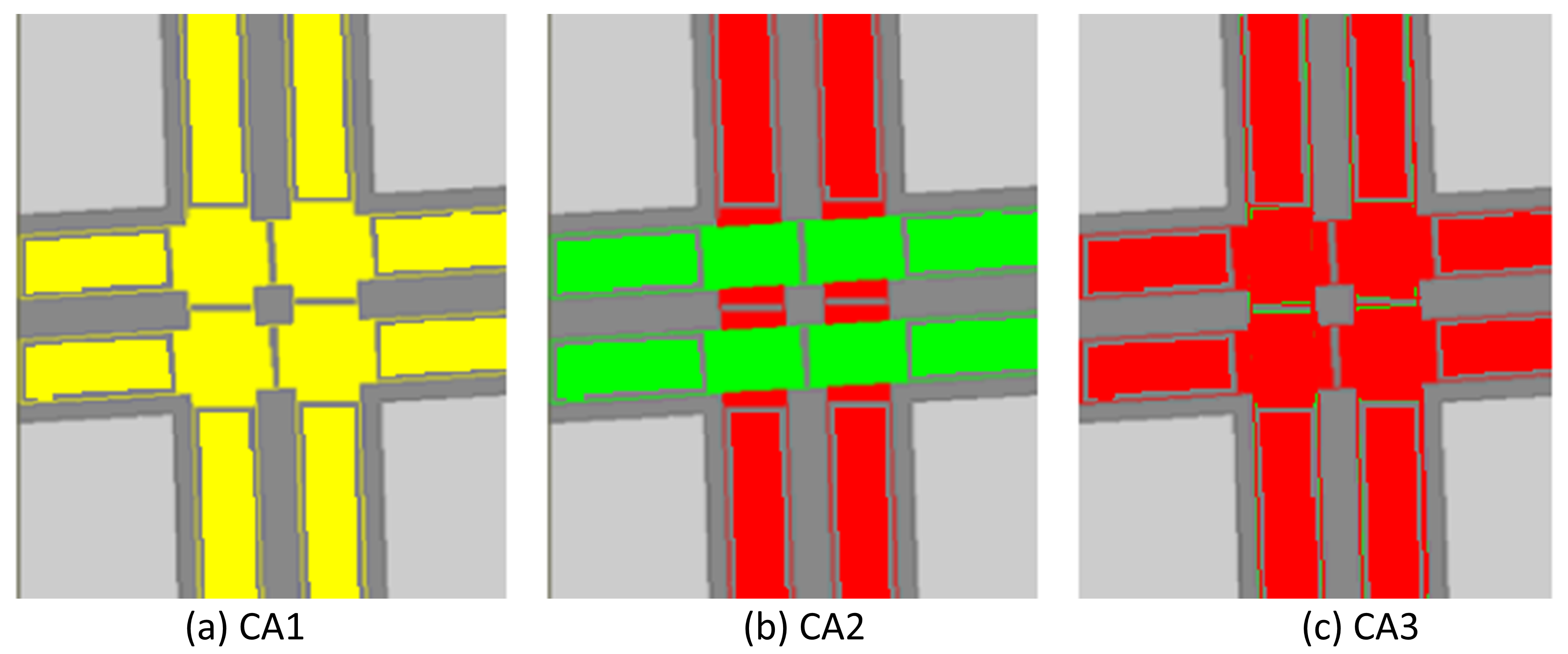
Figure 5: Different states of conflict areas.

The modeling approach for non-CAVs is summarized in Fig. 6, where blue arrows indicate mode (state) transitions. The driver switches from one mode to another as soon as a certain threshold is reached, usually expressed as a combination of speed difference and inter-vehicle distance.

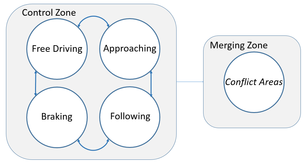
Figure 6: The Wiedemann model for non-CAVs.

V Energy Impact of CAV Penetration Under Different Traffic Scenarios

The energy impact study is carried out through a combination of MATLAB and VISSIM simulations. We consider a group of CAVs and non-CAVs crossing a single urban intersection, where the length of the CZ is $L=400$m and the length of the MZ is $S=30$m. For each direction, only one lane is considered. The minimum safe following distance is set to $\delta=10$m and the threshold for entering the AF mode is $\delta_{f}=10$m. The weights $w_{u}$ and $w_{s}$ in (11) are both set to 1. The vehicle arrivals are assumed to be given by a Poisson process and the initial speeds are uniformly distributed over $[10.9,11.1]$m/s.

V-A Energy Impact of CAV Penetration

We first compare the energy impact over different CAV penetration rates. Note that with 100% CAV penetration, all CAVs proceed according to the optimal trajectories determined in Sec. III and reach the MZ at the designated terminal times. However, for cases with less than 100% CAV penetration, we adopt the non-signalized collision avoidance rule (i.e., Conflict Areas) in mixed traffic, as non-CAVs may not follow the prescribed order in the queueing structure specified in Sec. II. The energy consumption with respect to different CAV penetration rates given the traffic flow rate set to $\lambda=700$ veh/(hour$\cdot$lane) is shown in Fig. 7. It can be seen that as the CAV penetration rate increases, the energy consumption decreases, which validates the efficiency of CAV penetration in terms of improving energy economy.

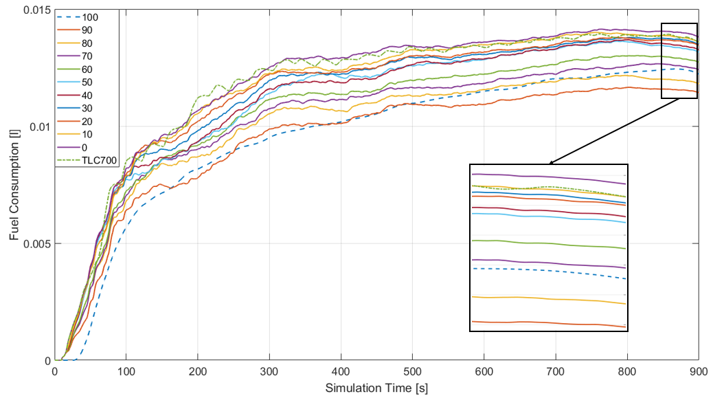
Figure 7: Energy consumption per second with respect to different CAV penetration rates given traffic flow rate set to $\lambda=$ 700 veh/(hour$\cdot$lane).

Observe in Fig. 7 that with no CAVs (0% penetration rate), the Conflict Areas cannot outperform the traffic light control case (indicated by TLC); however, with as little as 10% CAV penetration rate, TLC is outperformed. This leads to the conclusion that approximately 10% of vehicles should be CAVs before energy consumption performance can exceed that of TLC. However, this value clearly depends on traffic flow rates. Note that in Fig. 8(c) where the traffic flow rate is set to $\lambda=$ 750 veh/(hour$\cdot$lane), we need 90% of the vehicles to be CAVs in order to match the energy performance under TLC; in Fig. 8(a) and 8(b) where the traffic flow rates are set to $\lambda=500$ and $600$ veh/(hour$\cdot$lane) respectively, the cases with no CAVs (0% penetration) can easily outperform the TLC case; in Fig. 8(d) where $\lambda=800$ veh/(hour$\cdot$lane), all the vehicles have to be CAVs (100% penetration) in order to outperform the TLC case. Generally, higher CAV penetration is required to match the performance under TLC as traffic flow rate increases. The energy impact of traffic flow rates will be discussed in more details in Sec. V-B.

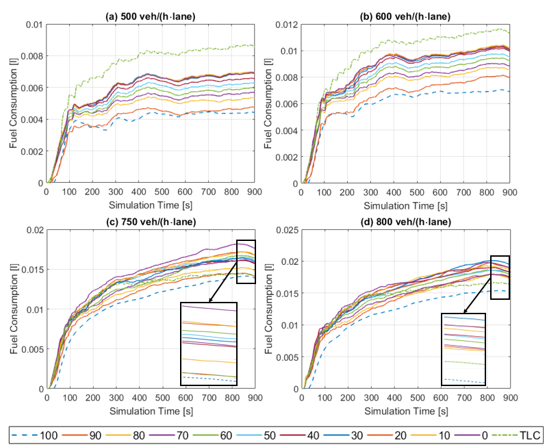
Figure 8: Energy consumption per second with respect to different CAV penetration rates given different traffic flow rates: (a) 500, (b) 600, (c) 750, (d) 800 veh/(hour$\cdot$lane).

An additional important observation is that energy performance is not always monotonically increasing with the penetration rate value. In Fig. 7, the energy consumption under 100% CAV penetration is actually worse than that with 90% and even 80% penetration rates. This is attributed to the overly conservative nature of our approach for determining the terminal time sequence, specifically the fact that only one vehicle is allowed inside the MZ at any time for vehicles traveling from different directions (4). On the other hand, the collision avoidance approach adopted under mixed traffic conditions (i.e., Conflict Areas) makes better use of the MZ by allowing vehicles to share it at the same time. Such more efficient MZ utilization reduces unnecessary travel delays.

V-B Energy Impact of CAV Penetration Under Different Traffic Flow Rates

For a dynamic system such as a transportation network, the performance should be measured while system stability is ensured, i.e., when the intersection is not saturated. When the intersection is saturated, it holds too many vehicles beyond its capacity and congestion would occur. In that case, it is not possible to apply any control except to use traffic signaling.

The saturation flow rate is an important concept for evaluating the performance of transportation systems, defined as the headway in seconds between vehicles moving at steady state. From the perspective of queueing theory, the intersection is a M/G/1 queue, where the MZ is the server and the vehicles are the clients. In order for the intersection to be stable, the vehicle arrival rate should be less than the MZ service rate, i.e., $\sum\lambda_{i}<\mu,$ where $\lambda_{i}$ is the arrival rate and $i$ is the index of different road segments, $\mu$ is the service rate of the MZ. According to the recursive structure of the terminal times in (5), for vehicles traveling on opposite roads, since they will not generate any collision inside the MZ, they are allowed to cross the MZ at the same time. Hence, we only need $\sum\lambda_{i}<2\cdot\mu$ to hold for the intersection to maintain stability. Assuming four symmetric road segments, i.e., $\lambda_{i}=\lambda,i\in\{1,2,3,4\}$, the saturation flow rate can be roughly estimated as $\lambda_{s}=900$ veh/(hour$\cdot$lane).

The volume-to-capacity ratio, also known as the degree of saturation, can be calculated by dividing the actual traffic flow rate by the saturation flow rate. Generally, an intersection with a degree of saturation less than 0.85 is considered under-saturated and typically has sufficient capacity to maintain a stable operation. The closer the degree of saturation is to 1, the more sensitive the system to the natural perturbation in traffic flow. When the degree of saturation exceeds 1, the intersection is described as over-saturated and there is nothing we can do except to use traffic signaling. Hence, to achieve the best performance, the traffic flow rate is set approximately under $\lambda_{c}$= 750 veh/(hour$\cdot$lane), where $\lambda_{c}$ is referred as the critical flow rate.

To explore the energy impact of CAV penetration with different traffic flow rates, a comparison is presented in Fig. 9 that shows the energy consumption with respect to both different CAV penetration rates and traffic flow rates. Observe that with lower traffic flow rates, that is, when the intersection is under-saturated (i.e., $\lambda<\lambda_{c}$), the benefit obtained from CAV penetration is more significant. Even the case with no CAVs can outperform the TLC case. With higher traffic flow rates, that is, when the degree of saturation of the intersection is near or over 1 (i.e., $\lambda>\lambda_{c}$), energy consumption can hardly gain any benefit from CAV penetration. In that case, even 100% CAV penetration cannot match the performance under TLC. This is consistent with our expectation: when the traffic is light, the red lights prevent some vehicles from crossing the intersection even if there is no other traffic that could generate collision inside the MZ; when the traffic is heavy, both CAVs and non-CAVs need to slow down or even stop to yield when they approach the MZ without traffic signaling and accelerate after they leave the intersection, which may consume more energy compared to the TLC case, where some vehicles do not need to stop during the green light phase.

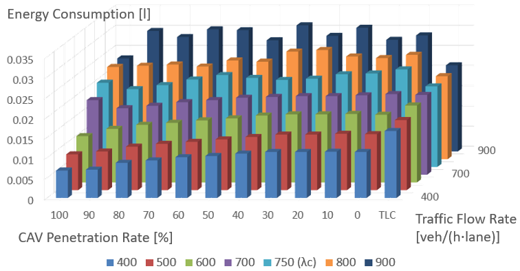
Figure 9: Average energy consumption with respect to both different traffic flow rates and CAV penetration rates.

The corresponding average travel times are shown in Fig. 10. Observe that before the traffic flow rate reaches the critical flow rate (i.e., $\lambda<\lambda_{c}$), the TLC cases are slightly outperformed in terms of travel times. This indicates that the non-signalized coordination policy (i.e., Conflict Areas) is more effective in terms of reducing travel delay compared to TLC. This may be due to the fact that the red lights prevent some vehicles from crossing the MZ even if there is no other traffic that could generate collision, while the non-signalized coordination policy makes better use of the MZ by allowing more vehicles sharing the MZ at the same time and hence reduces travel delay. When the traffic is heavy (i.e., $\lambda>\lambda_{c}$), almost all the vehicles have to slow down or even stop to yield when approaching the MZ without traffic signaling, which greatly increases the travel time.

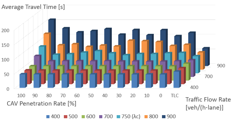
Figure 10: Average travel time with respect to different traffic flow rates and CAV penetration rates.

Overall, when the traffic is light, both the energy economy and the travel time can benefit from CAV penetration.

V-C Energy Impact of CAV Penetration Under Different Modeling Approaches

In addition to what has been discussed above, energy consumption can also be affected by how we model the vehicle behavior and the collision avoidance approach inside the MZ. Fig. 11 shows the energy consumption under different modeling approaches:

• For CAVs, the Wiedemann model is adopted for the AF mode (light blue bars), while for the collision avoidance method inside the MZ, we assume a fully controlled approach (CA3 in Fig. 5). Observe that the energy efficiency is improving as the CAV penetration rate increases. The benefit obtained from CAV penetration is consistent with what we have discussed in Sec. V-A.

• Based on scenario 1, we modify the collision avoidance method inside the MZ to a partially controlled approach (CA2 in Fig. 5), where some of the vehicles do not need to yield and hence, avoid unnecessary stops. Note that the stop-and-go process is one of the major reasons leading to extra energy consumption. The energy efficiency is improved (purple bars) compared with that under scenario 1, which indicates that more intelligent collision avoidance may save energy from reducing unnecessary stops and travel delay.

• Based on scenario 2, we apply the optimal control in terms of minimizing the energy consumption when CAVs are in the AF mode, while maintaining a minimum safety following distance $\delta$ with the preceding non-CAV if it exists. Observe that the energy performance under this case (green bars) outperforms that under scenario 2. This validates the effectiveness of our optimal control framework for CAVs.

• Based on scenario 2, we adopt a less aggressive Wiedemann car-following model by enabling the Smooth-Closeup option. This option forces the vehicle to decelerate in a gentle way when approaching the preceding vehicle, so as to reduce energy consumption and passenger discomfort, i.e., the jerk. As shown in the simulation results (red bars), the energy consumption decreases when Smooth-Closeup option is enabled.

• Based on scenario 4, we apply the optimal control in terms of minimizing the energy consumption when CAVs are in the AF mode, while maintaining a minimum safety following distance $\delta$ with the preceding non-CAV if it exists. Compared with scenario 4, the energy efficiency improves (dark blue bars) but the margin is not very significant. We may reach the conclusion that the Wiedemann car-following model with the Smooth-Closeup option enabled has a similar impact on energy economy as the optimal control for AF mode. This is intuitively correct in the sense that, the smoother the trip is, the less energy is consumed.

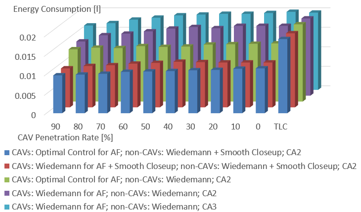
Figure 11: Energy consumption under different modeling approaches.

VI Concluding Remarks

Earlier work [22] has established a decentralized optimal control framework for optimally controlling CAVs crossing two adjacent intersections in an urban area. In this paper, we extended the solution of this problem to accommodate non-CAVs by formulating another optimal control problem to adaptively follow the preceding non-CAV. In addition, we investigate the energy impact of CAV penetration under different traffic scenarios. The simulation results validate the effectiveness of CAV penetration, and as the CAV penetration rate increases, the benefit becomes more significant. Such results can be consistently observed across a range of different traffic intensity settings as long as the traffic flow rate is below the critical flow rate; this provides strong evidence of the advantages of incorporating CAVs into current traffic systems.

Ongoing research is considering turns (see [24]) and lane changing in the intersection with a diverse set of CAVs and exploring the associated tradeoffs between the intersection throughput and energy consumption of each individual vehicle. Future research should also investigate the potential to further maximize the traffic throughput by re-evaluation of the vehicle crossing sequence as new vehicles enter the CZ.

References

- [1] J. L. Fleck, C. G. Cassandras, and Y. Geng, “Adaptive quasi-dynamic traffic light control,” IEEE Transactions on Control Systems Technology, 2015, DOI: 10.1109/TCST.2015.2468181, to appear.
- [2] W. Levine and M. Athans, “On the optimal error regulation of a string of moving vehicles,” IEEE Transactions on Automatic Control, vol. 11, no. 3, pp. 355–361, 1966.
- [3] K. Dresner and P. Stone, “Multiagent traffic management: a reservation-based intersection control mechanism,” in Proceedings of the Third International Joint Conference on Autonomous Agents and Multiagents Systems, 2004, pp. 530–537.
- [4] ——, “A Multiagent Approach to Autonomous Intersection Management,” Journal of Artificial Intelligence Research, vol. 31, pp. 591–653, 2008.
- [5] A. de La Fortelle, “Analysis of reservation algorithms for cooperative planning at intersections,” 13th International IEEE Conference on Intelligent Transportation Systems, pp. 445–449, Sept. 2010.
- [6] S. Huang, A. Sadek, and Y. Zhao, “Assessing the Mobility and Environmental Benefits of Reservation-Based Intelligent Intersections Using an Integrated Simulator,” IEEE Transactions on Intelligent Transportation Systems, vol. 13, no. 3, pp. 1201,1214, 2012.
- [7] L. Li and F.-Y. Wang, “Cooperative Driving at Blind Crossings Using Intervehicle Communication,” IEEE Transactions in Vehicular Technology, vol. 55, no. 6, pp. 1712,1724, 2006.
- [8] F. Yan, M. Dridi, and A. El Moudni, “Autonomous vehicle sequencing algorithm at isolated intersections,” 2009 12th International IEEE Conference on Intelligent Transportation Systems, pp. 1–6, 2009.
- [9] I. H. Zohdy, R. K. Kamalanathsharma, and H. Rakha, “Intersection management for autonomous vehicles using iCACC,” 2012 15th International IEEE Conference on Intelligent Transportation Systems, pp. 1109–1114, 2012.
- [10] F. Zhu and S. V. Ukkusuri, “A linear programming formulation for autonomous intersection control within a dynamic traffic assignment and connected vehicle environment,” Transportation Research Part C: Emerging Technologies, 2015.
- [11] J. Lee and B. Park, “Development and Evaluation of a Cooperative Vehicle Intersection Control Algorithm Under the Connected Vehicles Environment,” IEEE Transactions on Intelligent Transportation Systems, vol. 13, no. 1, pp. 81–90, 2012.
- [12] D. Miculescu and S. Karaman, “Polling-Systems-Based Control of High-Performance Provably-Safe Autonomous Intersections,” in 53rd IEEE Conference on Decision and Control, 2014.
- [13] J. Rios-Torres and A. A. Malikopoulos, “A Survey on the Coordination of Connected and Automated Vehicles at Intersections and Merging at Highway On-Ramps,” IEEE Transactions on Intelligent Transportation Systems, 2016 (forthcoming).
- [14] Y. Zhang, A. A. Malikopoulos, and C. G. Cassandras, “Optimal control and coordination of connected and automated vehicles at urban traffic intersections,” in Proceedings of the American Control Conference, 2016, pp. 6227–6232.
- [15] E. G. Gilbert, “Vehicle cruise: Improved fuel economy by periodic control,” Automatica, vol. 12, no. 2, pp. 159–166, 1976.
- [16] J. Hooker, “Optimal driving for single-vehicle fuel economy,” Transportation Research Part A: General, vol. 22, no. 3, pp. 183–201, 1988.
- [17] E. Hellström, J. Åslund, and L. Nielsen, “Design of an efficient algorithm for fuel-optimal look-ahead control,” Control Engineering Practice, vol. 18, no. 11, pp. 1318–1327, 2010.
- [18] S. E. Li, H. Peng, K. Li, and J. Wang, “Minimum fuel control strategy in automated car-following scenarios,” IEEE Transactions on Vehicular Technology, vol. 61, no. 3, pp. 998–1007, 2012.
- [19] K. M. Dresner and P. Stone, “Sharing the road: Autonomous vehicles meet human drivers.” in IJCAI, vol. 7, 2007, pp. 1263–1268.
- [20] S. I. Guler, M. Menendez, and L. Meier, “Using connected vehicle technology to improve the efficiency of intersections,” Transportation Research Part C: Emerging Technologies, vol. 46, pp. 121–131, 2014.
- [21] A. A. Malikopoulos, C. G. Cassandras, and Y. Zhang, “A decentralized energy-optimal control framework for connected automated vehicles at signal-free intersections,” Automatica, 2017 (to appear).
- [22] Y. Zhang, C. G. Cassandras, and A. A. Malikopoulos, “Optimal control of connected automated vehicles at urban traffic intersections: A feasibility enforcement analysis,” in Proceedings of the 2017 American Control Conference, 2017, pp. 3548–3553.
- [23] R. Wiedemann, “Simulation des strassenverkehrsflusses.” 1974.
- [24] Y. Zhang, A. A. Malikopoulos, and C. G. Cassandras, “Decentralized optimal control for connected automated vehicles at intersections including left and right turns,” in 56th IEEE Conference on Decision and Control, 2017, pp. 4428–4433.