Fine structure in holographic entanglement and entanglement contour
Abstract
We explore the fine structure of the holographic entanglement entropy proposal (the Ryu-Takayanagi formula) in AdS3/CFT2. With the guidance from the boundary and bulk modular flows we find a natural slicing of the entanglement wedge with the modular planes, which are codimension one bulk surfaces tangent to the modular flow everywhere. This gives an one-to-one correspondence between the points on the boundary interval and the points on the Ryu-Takayanagi (RT) surface . In the same sense an arbitrary subinterval of will correspond to a subinterval of . This fine correspondence indicates that the length of captures the contribution from to the entanglement entropy , hence gives the contour function for entanglement entropy. Furthermore we propose that in general can be written as a simple linear combination of entanglement entropies of single intervals inside . This proposal passes several nontrivial tests.
1 Introduction
The study of entanglement entropy, which describes the correlation structure of a quantum system, has played a central role in the study of modern theoretical physics in the last decade. Large amount of interest is stimulated by the Ryu-Takayanagi (RT) Ryu:2006bv ; Ryu:2006ef formula in the context of AdS/CFT correspondence Maldacena:1997re ; Gubser:1998bc ; Witten:1998qj . More explicitly, for a static subregion in the boundary CFT and a minimal surface in the dual AdS bulk that anchored on the boundary of , the RT formula states that the entanglement entropy of is measured by the area of in Planck units,
| (1.1) |
The covariant version of the RT formula is proposed in Hubeny:2007xt with the minimal surface generalized to the extremal surface.
The are two main strategies to derive the RT formula based on the AdS/CFT. The first one is the Rindler method whose physical logic is first proposed in Casini:2011kv . Later the authors of Song:2016gtd ; Jiang:2017ecm find a general way to construct Rindler transformations using the symmetries of the quantum field theory thus generalize the Rindler method to holographic models beyond AdS/CFT. The key point of the Rindler method is to construct a Rindler transformation which is a symmetry of the theory and maps the causal development of a subregion to a thermalized “Rindler space”. Thus the problem of calculating the entanglement entropy is replaced by the problem of calculating the thermal entropy of the Rindler space. According to holography, the thermal entropy of the Rindler space is given by the thermal entropy of its bulk dual, which is just a hyperbolic black hole. The horizon of the hyperbolic black hole is exactly what maps to the RT surface under the bulk extended Rindler transformations. An useful by-product of the Rindler method is the picture of boundary and bulk modular flows (see Jiang:2017ecm ), which play a crucial role in this paper.
The second way is the Lewkowycz-Maldacena (LM) prescription Lewkowycz:2013nqa (see Dong:2016hjy for its covariant generalization) which extend the replica trick Calabrese:2004eu into the bulk, and calculate the entanglement entropy using the on-shell partition function on the replicated bulk geometry. The entanglement entropy is defined as the von Neumann entropy of the reduced density matrix . Consider a quantum field theory on , the replica trick first calculate the Rényi entropy for , then analytically continue away from integers. When , we get the entanglement entropy . To calculate , we cut open along , glue n copies of them cyclically, then do path integral on the newly glued manifold . The entanglement entropy is calculated by
| (1.2) |
where is the partition function of the quantum field theory on . Assuming holography and the unbroken replica symmetry in the bulk, the LM prescription manages to construct the bulk dual of , which is a replicated bulk geometry with its boundary being . Then can be calculated by path integral on on the gravity side.
In this paper, based on the above two stories, we explore the fine correspondence between the points on the boundary interval and the points on the according RT surface with the guidance of modular flows. Then we relate the fine structure to the entanglement contour, which characterizes the spatial structure of entanglement entropy.
2 Boundary and bulk modular flows
We consider a straight interval
| (2.3) |
at the boundary of the Poincaré AdS3
| (2.4) |
Here we have set the AdS radius . We can go back to the usual Poincaré coordinates by setting
| (2.5) |
The causal development of is given by
| (2.6) |
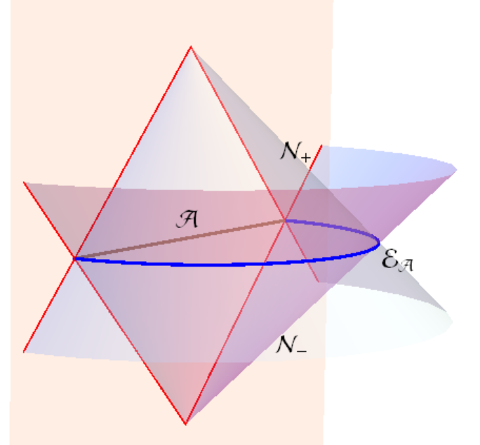
Accordingly the extremal surface and the corresponding two normal null hypersurfaces are given by
| (2.7) | ||||
| (2.8) |
The entanglement wedge Headrick:2014cta is the bulk region enclosed by and .
Following the strategy in Jiang:2017ecm , we can construct a Rindler transformation on the boundary, which is a conformal mapping that maps to a Rindler space with coordinates () and infinitely faraway boundary. The strategy requires the translation along the new coordinates to be a linear combination of the global generators of the boundary CFT. Since the global generators are dual to the bulk isometries, we can naturally extend the Rindler transformations into the bulk by replacing the global generators of the CFT with the isometries of AdS3. The bulk extended Rindler transformations map the entanglement wedge to the exterior of the uncompactified horizon of a Rindler spacetime with a thermal circle .
We can write the reduced density matrix as , where is known as the modular Hamiltonian. The state in the Rindler space is a thermal state with the thermal density matrix , where and is the ordinary Hamiltonian in . The modular flow in is just the ordinary time translation along the thermal circle . Similarly we can extend into the bulk and get a bulk modular flow . With the inverse Rindler transformations, we get the bulk and boundary modular flows,
| (2.9) | ||||
| (2.10) | ||||
| (2.11) |
which is generated by the modular Hamiltonian in the original Poincaré AdS3. We present the details of the Rindler transformations and the derivation of modular flows in Appendix A. It is easy to check that , which indicates the extremal surface is the fixed points of the bulk modular flow (or bulk replica symmetry).
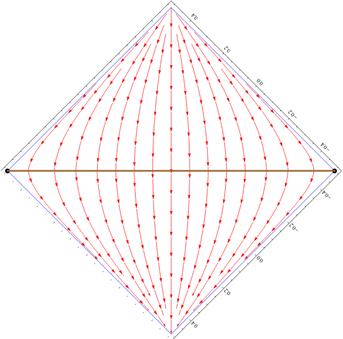
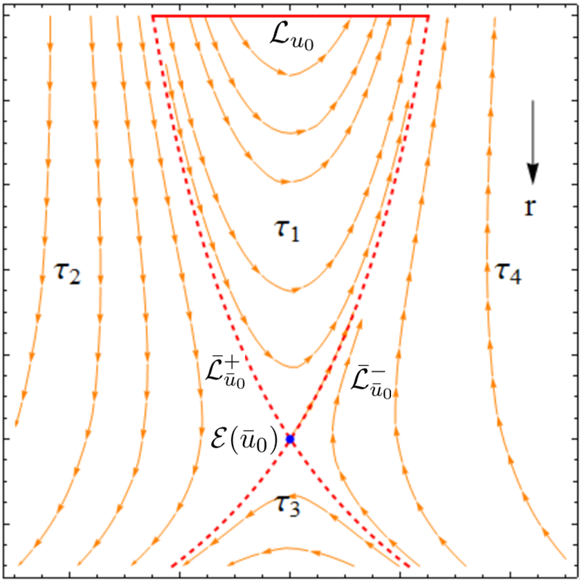
Solving the equations and respectively, we can get the functions of the modular flow lines both on the boundary and in the bulk. From now on we consider the static case with . On the boundary, up to a reparametrization, the modular flow lines are given by
| (2.14) |
where parametrizes and characterize different modular flow lines by being the coordinate of the point where intersect with (see the left figure in Fig.1). In the bulk, one can easily check that the normal null geodesics on (which is also studied in Headrick:2014cta ) are also modular flow lines in the bulk, which are given by (for details see Appendix B)
| (2.17) | |||
| (2.20) |
where characterize different modular flow lines by being the coordinate of the point where intersect with .
3 Slicing the entanglement wedge with modular planes
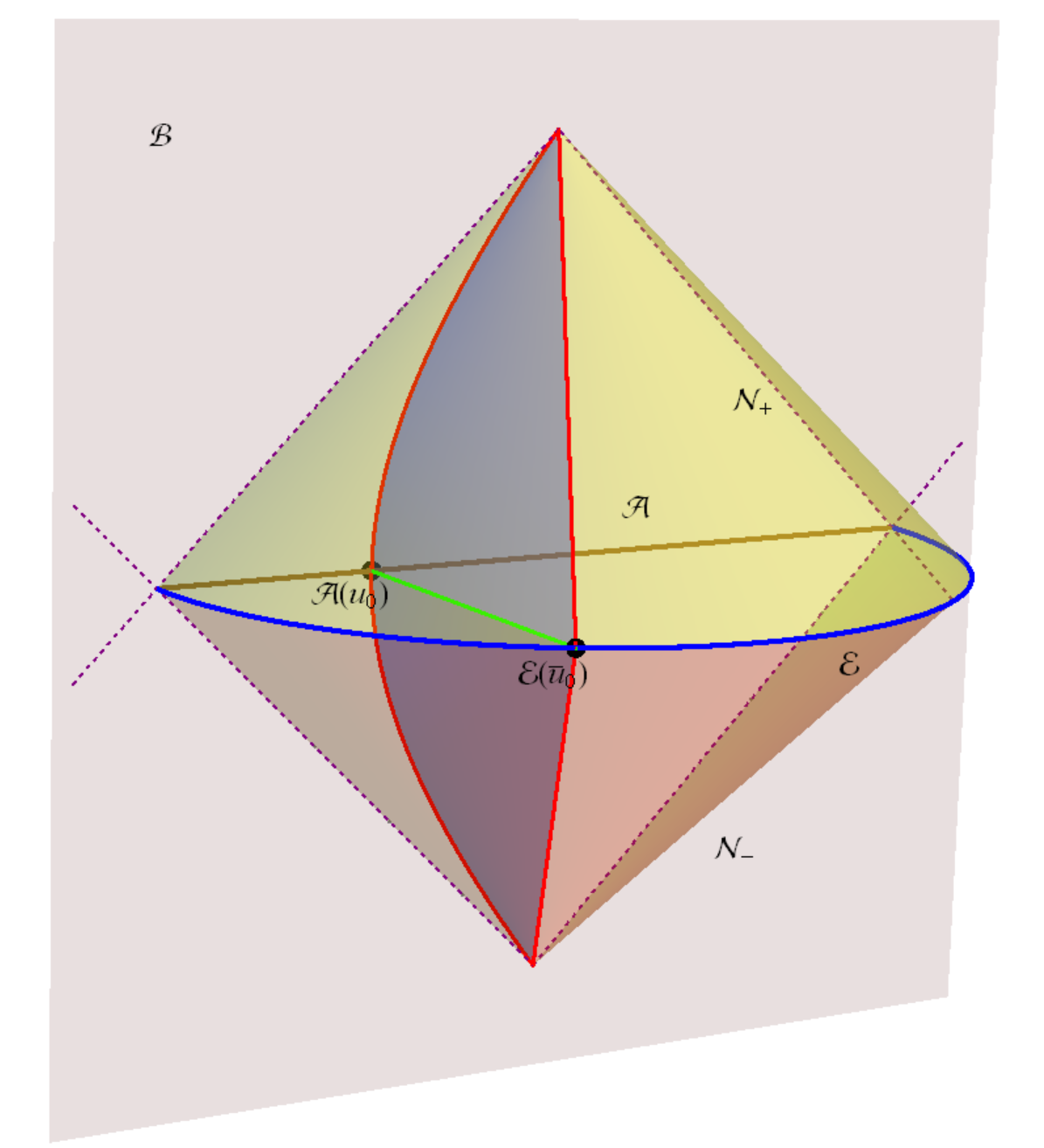
For a given with , we define the modular plane as the orbit of the boundary modular flow line under the bulk modular flow. is a codimension one surface in the bulk (see the right figure in Fig.1). It is nice to know that for every point on , its orbit under will return back to on another point, which indicates that and are in one-to-one correspondence. With and known, the modular plane can be uniquely determined. We define the two points
| (3.21) | ||||
| (3.22) |
as the points where intersect with and respectively (see Fig.2). By definition we have
| (3.23) |
Define the homology surface as a codimension one spacelike surface in which satisfies . The prescription of Dong:2016hjy to construct the corresponding bulk replicated geometry is in the following. Firstly, for each copy of bulk , where denote the th copy of the bulk, we cut them open along to and . Then we get the replicated geometry by gluing the open cuts cyclically
| (3.24) |
Similar to Dong:2016hjy , we use bulk Rindler coordinates to denote all the bulk regions. We allow to be complex and refer to all the bulk regions in question by using
| (3.25) |
Here parameterizes the modular flow in the bulk with a thermal circle . Note that when we translate along a modular flow, only Re changes while Im is fixed. When we apply the replica trick in the bulk, the orbit of modular flows changes accordingly as well as the distribution of Im.
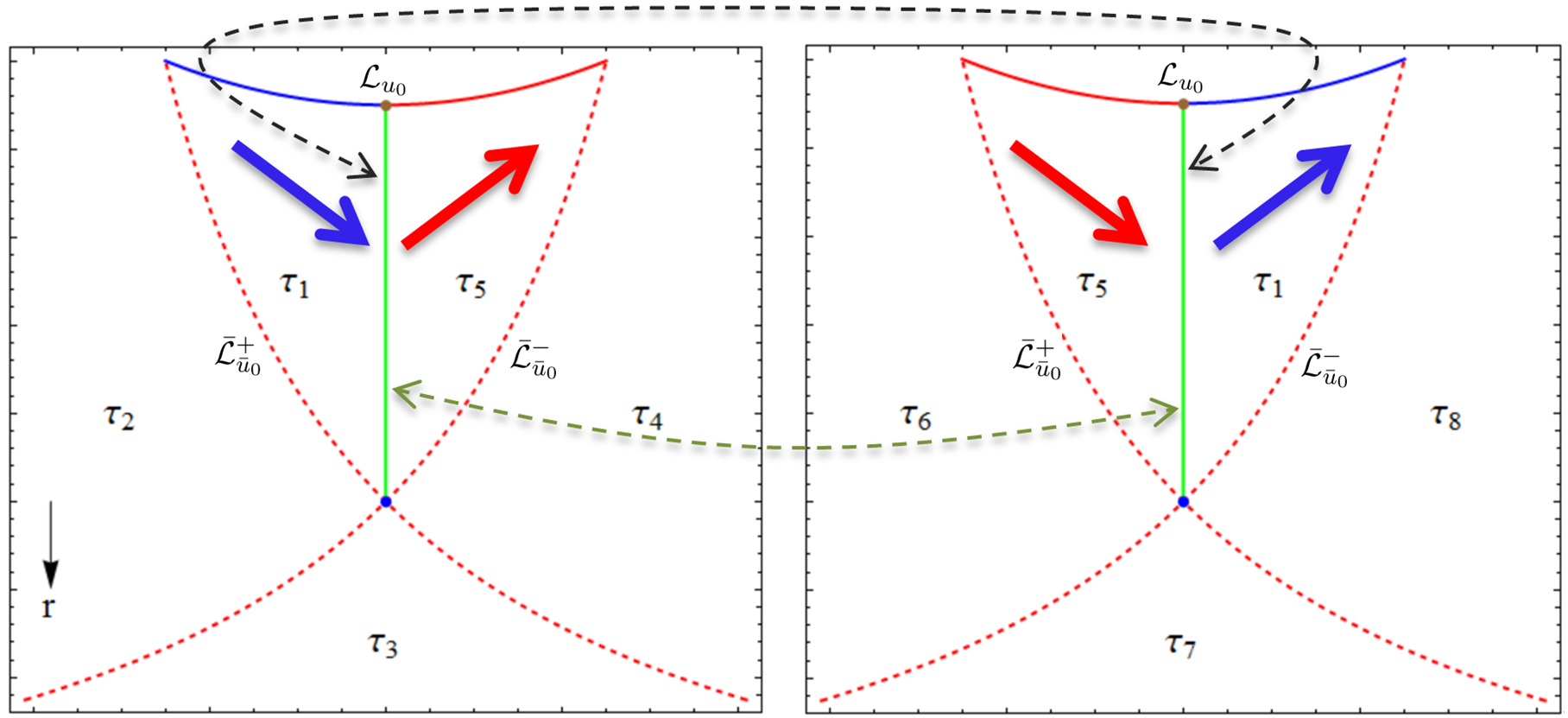
Let us focus on the cyclic gluing of one point on . On the boundary passes through then enter the next copy of . The natural bulk extension of the cyclic gluing of should be the cyclic gluing of on the modular planes, where . In other words, we cut open along to and then impose the following boundary conditions
| (3.26) |
where denotes all the bulk metric and matter fields. Note that the definition of modular plane indicates that all the bulk modular flow lines emanate from always lie in . Following the modular flows we can keep track of the value of Im everywhere on the cyclically glued modular plane (see Fig.3 for the case of ). We find that the cyclic gluing of on the boundary induces a thermal circle on .
In summary, following the modular flow, the cyclic gluing of a point on the boundary interval effectively induces a replica story on the corresponding modular plane . Following the calculation in Lewkowycz:2013nqa ; Dong:2016hjy , this turns on nonzero contribution to the entanglement entropy on . The whole bulk replica story can be considered as a slicing of replica stories on all the modular planes. In this sense a point on the boundary interval is related to a unique point on the RT surface. For the specific choice of as a straight interval, we find the two points in (3.21) are related by (for details see Appendix B)
| (3.27) |
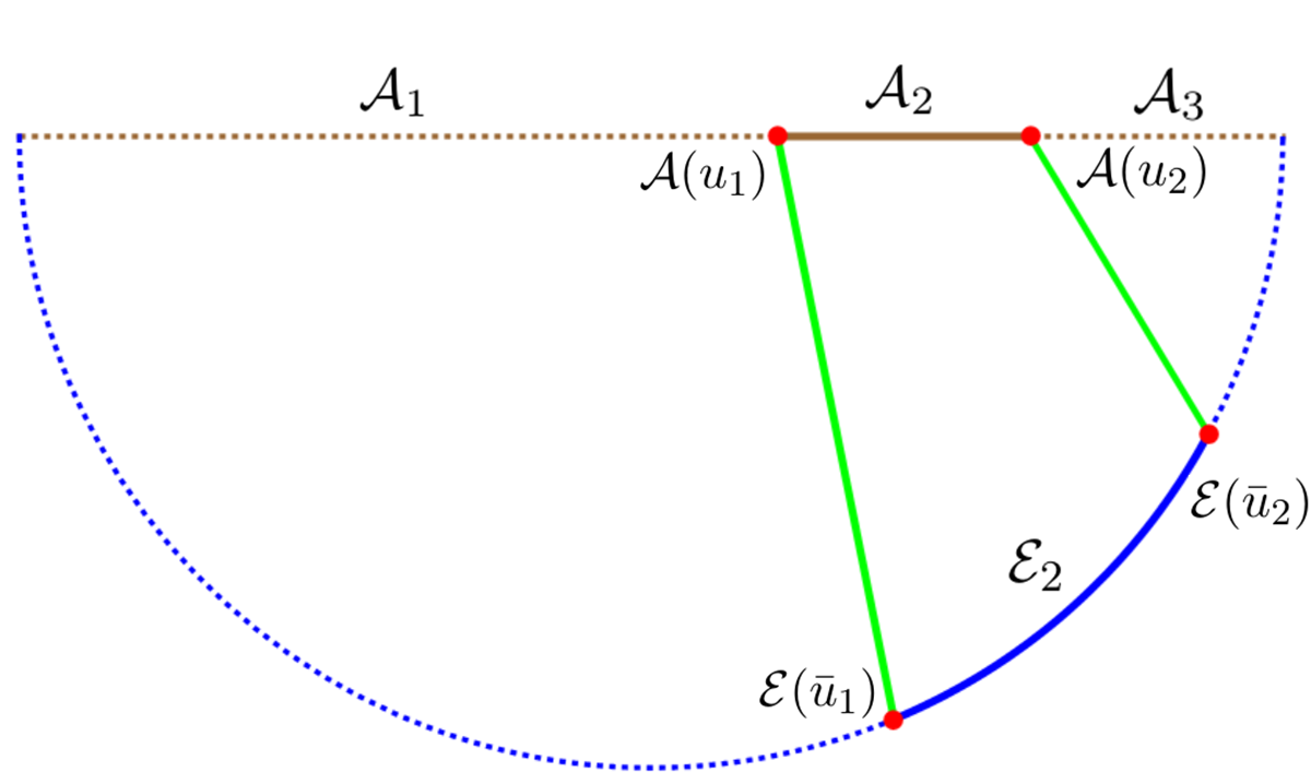
We want to address that, according to our prescription the cyclic gluing of an arbitrary point on would induce the same replica story on . In other words correspond to all the points on in the same sense as .
4 Entanglement contour from the fine structure
In the same sense, the cyclic gluing of an arbitrary subinterval on turns on the contribution to the entanglement entropy from the subinterval of the RT surface (see the left figure of Fig.4). We use to denote the length of the intervals and respectively. It is natural to propose that captures the contribution from to the entanglement entropy . In other words we get the contour function for which describes the distribution of contribution to entanglement from each point of and satisfies
| (4.28) |
The authors of Vidal proposed a set of requirements for the contour functions. Few analysis of the contour functions for bipartite entanglement have been explored in Botero ; Vidal ; PhysRevB.92.115129 ; Coser:2017dtb ; Tonni:2017jom . However the complete list of requirements that uniquely determines the contour is still not available. Also its fundamental definition is still not established. Our fine structure analysis gives a holographic definition for the contour function. According to (3.27) we have
| (4.29) |
which is consistent with the results in Vidal ; Coser:2017dtb . Also we get
| (4.30) | ||||
where we have used . In Appendix C, we compare with the mutual information and show that they are not the same thing.
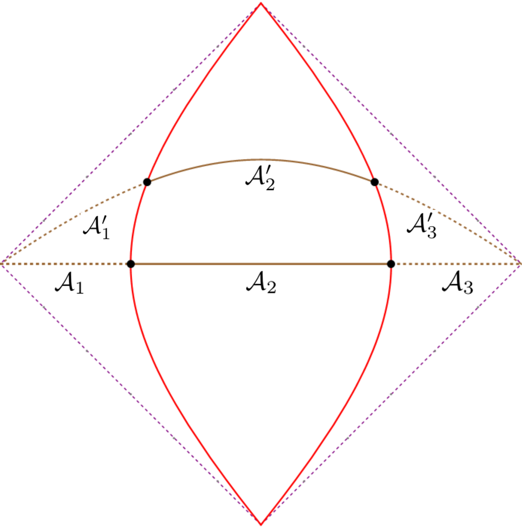
We consider as an arbitrary spacelike interval homologous to , and as the subinterval that ends on the same two modular flow lines and as (see the right figure of Fig.4). Since and go through the same modular planes, according to our prescription, they should both correspond to , thus we should have
| (4.31) |
which means the entanglement contour is invariant under the boundary modular flow. This requirement should be satisfied in more general cases with locally defined modular Hamiltonians, and is new compared with the requirements in Vidal .
It is also interesting to consider the limit , as expected we find
| (4.32) |
Under this limit the property (4.31) naturally reduce to the causal property of entanglement entropy. Note that the proposal = Casini:2008wt that involves mutual information can not reproduce the right causal property of . The points and , where is cut off, satisfy , thus relates the boundary and bulk cutoffs in a natural way. This is because the modular planes are defined in a holographic way.
5 A simple proposal for the contour function
One interesting observation in our special case is that can be expressed as a linear combination of the entanglement entropy of single intervals inside
| (5.33) |
Here we would like to propose that the above simple combination gives the contour function of entanglement entropy in general 1+1 dimensional theories. We will show that:
-
1.
defined by (5.33) is in general additive by definition, and positive from strong subadditivity Lieb:1973zz ; Lieb:1973cp ,
- 2.
-
3.
it also reproduces the right contour function for CFT2 with a thermal (spatial) circle, and Warped CFT Wen:2018mev .
Furthermore Vidal requires the contour function to satisfy a constraint implementing the consistency with any spatial symmetry of the subsystem, and a bound meaning that must be smaller or equal than the entanglement of any factor space of which contains the Hilbert space of . We leave these for future discussions.
For quantum systems whose entanglement entropies satisfy the volume law, the proposal (5.33) gives a flat entanglement contour function. For systems that satisfy area law, (5.33) also captures the feature that the leading order contribution to the entanglement entropy comes from the boundary.
5.1 Additivity and positivity
We can divide the subinterval into two parts such that
| (5.35) |
According to (5.33) we have
| (5.36) | ||||
| (5.37) |
then we find that
| (5.38) |
We can continue to do the division such that is divided into all the sites inside , the additivity actually determines a function on that does not depend on the choice of and satisfies
| (5.39) |
Further more, since
| (5.40) |
we have
| (5.41) |
which is a crucial property for the contour function.
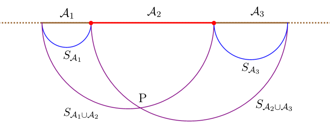
The positivity of is directly given by the strong subadditivity. For example, if we consider holographic CFT2 and a static interval , we see from Fig.5 that Headrick:2007km
| (5.42) |
According to (5.33) and the additivity, the above inequality indicates that the contour function is positive everywhere inside
| (5.43) |
Note that we only used the definition (5.33) of and the strong subadditivity of entanglement entropy, so the above properties (5.41) and (5.43) of (5.33) should hold for general cases.
5.2 Invariance under local unitary transformations and the modular flow
The causal property of entanglement entropy tells us that and are invariant under local unitary transformations that only acts on the subset , then the defined by (5.33) is also invariant under thus satisfies the requirement of Vidal . Furthermore, (5.33) is also invariant under the local unitary transformations and .
Our fine structure analysis indicates that even under modular flow, the contour function should be invariant in the sense of (4.31). Remarkably we show that the defined by (5.33) is also invariant under the modular flow in our special case. According to (A.78), the entanglement entropy for an arbitrary interval is determinant by the coordinate differences of the two endpoints
| (5.44) |
Now we consider an arbitrary spacelike interval which is homologous to and intersect with and at
5.3 Reproducing the contour function for CFT2 with a thermal (spatial) circle
Here we consider a CFT2 with the inverse temperature . The entanglement entropy for an arbitrary static interval is given by
| (5.51) |
where is the length of the interval. According to (5.33) we have
| (5.52) |
Define , then we should have
| (5.53) |
where
| (5.54) |
are the two endpoints of . It is easy to see that (5.52) can be written in the form of (5.53) with given by
| (5.55) |
Thus we get the contour function for CFT2 with finite temperature
| (5.56) |
Similarly we can get the contour function for the zero temperature CFT2 with a spatial circle ,
| (5.57) |
The above results (5.56) and (5.57) are consistent with the results proposed in Coser:2017dtb , which are also inspired by the locally defined modular Hamiltonian Bisognano:1975ih ; Bisognano:1976za ; Casini:2011kv ; Cardy:2016fqc .
6 Discussion
The modular Hamiltonian absolutely contains more information than the entanglement entropy. This work shows that a fine correspondence between quantum entanglement and space-time geometry can be extracted from the RT formula by the bulk and boundary modular flows. This fine correspondence is indeed the holographic picture of the entanglement contour, which probes the locality of entanglement and gives more information (see discussions in Vidal ) than the total entanglement entorpy. Our prescription, although it relies on the construction of Rindler transformations, should work for general cases with a locally defined modular Hamiltonian, for example, the covariant case by setting , the global AdS3, AdS3 with a black hole, AdS space in higher dimensions (for spherical subregions Rindler transformations has been constructed in Casini:2011kv ), and even the cases Song:2016gtd ; Jiang:2017ecm beyond AdS/CFT (see Wen:2018mev for another explicit case in the context of warped AdS3/warped CFT correspondence Detournay:2012pc ). For cases with nonlocal modular Hamiltonian, one may find clues from the more general discussions on bulk and boundary modular flows in Faulkner:2013ana ; Jafferis:2015del ; Faulkner:2017vdd to define the modular planes in a more abstract way.
On the other hand we give a simple proposal (5.33) for the entanglement contour function for general cases, which only involves entanglement entropies of single subintervals inside and does not depend on the construction of the Rindler transformations. It also passes several nontrivial tests. The fine correspondence in holographic entanglement together with the proposal (5.33) allow us to interpret the length of bulk intervals in terms of entanglement entropies of the dual field theory (see Abt:2018ywl for a recent application along this line). On the other way around, we can get the information of the modular flow from the entanglement entropy based on this proposal.
The fine structure also gives a good explanation Wen:2018mev for the appearance of null geodesics in the new geometric pictures Song:2016gtd ; Jiang:2017ecm of entanglement entropy in non-AdS holographies. The RT formula has a very deep impact on our understanding of holography itself and the origin of spacetime geometry Swingle:2009bg ; VanRaamsdonk:2009ar ; VanRaamsdonk:2010pw ; Maldacena:2013xja . Its fine description111Another attempt to obtain a fine description of the RT formula is given by Freedman:2016zud using a tool named “bit threads” which represent entanglement between points on the boundary. may help us better understand these grand questions.
ACKNOWLEDGMENTS
We thank Ping Gao, Temple He, Hongliang Jiang, Aitor Lewkowycz and Mukund Rangamani for helpful discussions. Especially we would like to thank Matthew Headrick and Wei Song for insightful discussions. We also thank Shiu-Yuen Cheng, Wei Song, Shing-Tung Yau and Pin Yu for support. This work is supported by NSFC Grant No.11805109.
Appendix A Rindler method and modular flows in AdS3/CFT2
The general strategy to construct Rindler transformations and their bulk extensions by using the symmetries of a QFT and holographic dictionary, is summarised in Sec. 2 of Jiang:2017ecm . In the case of AdS3/CFT2, the Rindler transformations are constructed by imposing the following requirements
-
•
The Rindler transformation should be a symmetry transformation, which, in this case, is a conformal mapping
(A.58) with and being arbitrary functions.
-
•
The vectors should be a linear combination of the global generators in the original CFT. In other words
(A.59) where are arbitrary constants.
-
•
The bulk extension of the Rindler transformation is obtained by replacing the global generators in (A.59) with their bulk duals, which are just the isometries of the Poincaré AdS3. Furthermore we require the metric of the Rindler to satisfy the same boundary conditions.
The global generators of the boundary CFT2 are and , whose bulk dual are the isometries of the Poincaré AdS3
| (A.60) | |||
| (A.61) |
The normalization are chosen to satisfy the standard algebra
| (A.62) | |||
| (A.63) |
Now we try to construct a Rindler coordinate transformation that satisfies the above requirements, to obtain a new coordinate system. Define
| (A.64) | |||
| (A.65) |
where are arbitrary constants which controls the size, position of on and the two parameters that characterize the thermal circle in . Note that the shape of is determined by the symmetries of the CFT thus can not be adjusted. Only the two parameters that characterize the size of can affect the entanglement entropy. Furthermore by requiring the metric of the Rindler to have the formula of (A.69) , or equivalently , determines the other coordinate .
For simplicity we can settle down the position of and the thermal circle of the Rindler . This leaves only two parameters and , which characterize the size of . By choosing
| (A.66) | |||
| (A.67) |
we find the bulk Rindler transformations from Poincaré AdS3
| (A.68) |
to a Rindler
| (A.69) |
are given by
| (A.70) | ||||
| (A.71) | ||||
| (A.72) |
Here we have set down the parameters and the position of , which do not affect the entanglement entropy. Asymptotically, we have
| (A.73) |
which is as expected a conformal mapping. The coordinates covers a diamond shape subregion on the original coordinates
| (A.74) |
which is the causal development of the interval
| (A.75) |
on the boundary CFT. The causal development (A.74) constructed by only using Rindler transformations is consistent with the causal development defined with null lines associated to on .
According to (A.72), the horizon of the Rindler at maps to two null hypersurfaces in the original space
| (A.76) |
We see that intersect at
| (A.77) |
which anchors on the boundary endpoints . It is easy to check that the is just the extremal surface. The entanglement entropy is given by
| (A.78) |
where and are the cutoffs along the and directions.
On the other hand, one can also check that the normal null hypersurfaces emanating from (A.77) are just (A.76). This means the normal null hypersurfaces of play the role of the horizon in Rindler . The above picture is just the light-sheet Bousso:2002ju construction of the HRT surface first proposed in Hubeny:2007xt . The entanglement wedge is the bulk region enclosed by and . The Rindler transformation (A.70) maps this to the exterior of the horizon in Rindler . The bulk causal decomposition associate with is given by the left figure in Fig.6. It is easy to see that the followed boundary decomposition is consistent with the causal structure for a CFT2, which is given by the right figure of Fig.6.
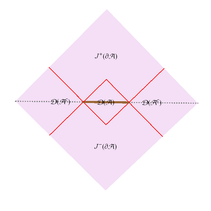
The generator of the normal Hamiltonian in Rindler space or Rindler bulk (A.69), which maps to the modular Hamiltonian in the original space, is the generator along the thermal circle . In order to map it to the original space, we need to solve the following differential equations
| (A.79) | ||||
| (A.80) | ||||
| (A.81) |
Then we get , and furthermore , in terms of .
We plug the bulk Rindler transformations (A.70) into the differential equations (A.79) then solve them. In Rindler the generator of the Hamiltonian is just the translation along the thermal circle. Mapping it to the original space, we get the modular flow in the bulk
| (A.82) | |||||
| (A.83) | |||||
| (A.84) | |||||
| (A.85) | |||||
The modular flow on the boundary is given by
| (A.86) |
One can easily check that
| (A.87) |
The above equations mean that is the fixed points of (or the bulk extended replica symmetry), and should go through the endpoints of the boundary interval.
Appendix B Details to derive the equations (11) (12) and (18)
B.1 Normal null geodesics on as bulk modular flow lines
One can check that the following bulk flow lines
| (B.88) |
satisfy the equation , where is an integration constant. These are the bulk modular flow lines on , one can also check that they are the null geodesics normal to , which are also studied in Headrick:2014cta .
B.2 Deriving equation (3.27)
On the real boundary , all the bulk modular flow lines (2.17) intersect with the boundary modular flow lines (2.14) at the tips of the casual development . Our construction of modular planes indicates that for each boundary modular flow line , there are two bulk modular flow lines on that lie in the same modular plane . To get the relation (3.27), we need to push the boundary with modular flows (2.14) to a finite , then for each there will be a that intersect with at some finite . More explicitly we solve the equation
| (B.93) | ||||
| (B.94) |
and get the intersecting point at
| (B.95) | ||||
| (B.96) |
Then we take the limit and get
| (B.97) | ||||
| (B.98) |
which give the relation (3.27).
Appendix C Entanglement contour compared with mutual information
We define and compare it with the mutual information
| (C.99) |
which is claimed to capture the correlation between and . The evaluation of the mutual information involves the calculation of the entanglement entropy of two disconnected intervals, which is still a formidable task. If we follow the proposal of Calabrese:2004eu ; Hubeny:2007re
| (C.100) |
then we find exactly which holds for general . Though there do exist cases Casini:2004bw ; Casini:2005rm ; Casini:2008wt ; Casini:2009vk that apply (C.100), it is shown in the added note of Calabrese:2004eu that the result is in general not correct.
One may also calculate by applying the RT formula to two disconnected intervals as advocated in Headrick:2010zt thus the mutual information (C.99) is given by
| (C.103) |
which undergoes a phase transition at . When we have the simple relation
| (C.104) |
However this relation does not hold for general , because (C.103) is not invariant under the modular flow.
References
- (1) S. Ryu and T. Takayanagi, Holographic derivation of entanglement entropy from AdS/CFT, Phys. Rev. Lett. 96 (2006) 181602, [hep-th/0603001].
- (2) S. Ryu and T. Takayanagi, Aspects of Holographic Entanglement Entropy, JHEP 08 (2006) 045, [hep-th/0605073].
- (3) J. M. Maldacena, The Large N limit of superconformal field theories and supergravity, Int. J. Theor. Phys. 38 (1999) 1113–1133, [hep-th/9711200].
- (4) S. S. Gubser, I. R. Klebanov and A. M. Polyakov, Gauge theory correlators from noncritical string theory, Phys. Lett. B428 (1998) 105–114, [hep-th/9802109].
- (5) E. Witten, Anti-de Sitter space and holography, Adv. Theor. Math. Phys. 2 (1998) 253–291, [hep-th/9802150].
- (6) V. E. Hubeny, M. Rangamani and T. Takayanagi, A Covariant holographic entanglement entropy proposal, JHEP 07 (2007) 062, [0705.0016].
- (7) H. Casini, M. Huerta and R. C. Myers, Towards a derivation of holographic entanglement entropy, JHEP 05 (2011) 036, [1102.0440].
- (8) W. Song, Q. Wen and J. Xu, Modifications to Holographic Entanglement Entropy in Warped CFT, JHEP 02 (2017) 067, [1610.00727].
- (9) H. Jiang, W. Song and Q. Wen, Entanglement Entropy in Flat Holography, JHEP 07 (2017) 142, [1706.07552].
- (10) A. Lewkowycz and J. Maldacena, Generalized gravitational entropy, JHEP 08 (2013) 090, [1304.4926].
- (11) X. Dong, A. Lewkowycz and M. Rangamani, Deriving covariant holographic entanglement, JHEP 11 (2016) 028, [1607.07506].
- (12) P. Calabrese and J. L. Cardy, Entanglement entropy and quantum field theory, J. Stat. Mech. 0406 (2004) P06002, [hep-th/0405152].
- (13) M. Headrick, V. E. Hubeny, A. Lawrence and M. Rangamani, Causality & holographic entanglement entropy, JHEP 12 (2014) 162, [1408.6300].
- (14) Y. Chen and G. Vidal, Entanglement contour, Journal of Statistical Mechanics: Theory and Experiment 2014 (2014) P10011, [1406.1471].
- (15) A. Botero and B. Reznik, Spatial structures and localization of vacuum entanglement in the linear harmonic chain, Phys. Rev. A 70 (Nov, 2004) 052329.
- (16) I. Frérot and T. Roscilde, Area law and its violation: A microscopic inspection into the structure of entanglement and fluctuations, Phys. Rev. B 92 (Sep, 2015) 115129.
- (17) A. Coser, C. De Nobili and E. Tonni, A contour for the entanglement entropies in harmonic lattices, J. Phys. A50 (2017) 314001, [1701.08427].
- (18) E. Tonni, J. Rodriguez-Laguna and G. Sierra, Entanglement hamiltonian and entanglement contour in inhomogeneous 1D critical systems, J. Stat. Mech. 1804 (2018) 043105, [1712.03557].
- (19) H. Casini and M. Huerta, Remarks on the entanglement entropy for disconnected regions, JHEP 03 (2009) 048, [0812.1773].
- (20) E. H. Lieb and M. B. Ruskai, A Fundamental Property of Quantum-Mechanical Entropy, Phys. Rev. Lett. 30 (1973) 434–436.
- (21) E. H. Lieb and M. B. Ruskai, Proof of the strong subadditivity of quantum-mechanical entropy, J. Math. Phys. 14 (1973) 1938–1941.
- (22) Q. Wen, Towards the generalized gravitational entropy for spacetimes with non-Lorentz invariant duals, 1810.11756.
- (23) M. Headrick and T. Takayanagi, A Holographic proof of the strong subadditivity of entanglement entropy, Phys. Rev. D76 (2007) 106013, [0704.3719].
- (24) J. J. Bisognano and E. H. Wichmann, On the Duality Condition for a Hermitian Scalar Field, J. Math. Phys. 16 (1975) 985–1007.
- (25) J. J. Bisognano and E. H. Wichmann, On the Duality Condition for Quantum Fields, J. Math. Phys. 17 (1976) 303–321.
- (26) J. Cardy and E. Tonni, Entanglement hamiltonians in two-dimensional conformal field theory, J. Stat. Mech. 1612 (2016) 123103, [1608.01283].
- (27) S. Detournay, T. Hartman and D. M. Hofman, Warped Conformal Field Theory, Phys. Rev. D86 (2012) 124018, [1210.0539].
- (28) T. Faulkner, A. Lewkowycz and J. Maldacena, Quantum corrections to holographic entanglement entropy, JHEP 11 (2013) 074, [1307.2892].
- (29) D. L. Jafferis, A. Lewkowycz, J. Maldacena and S. J. Suh, Relative entropy equals bulk relative entropy, JHEP 06 (2016) 004, [1512.06431].
- (30) T. Faulkner and A. Lewkowycz, Bulk locality from modular flow, JHEP 07 (2017) 151, [1704.05464].
- (31) R. Abt, J. Erdmenger, M. Gerbershagen, C. M. Melby-Thompson and C. Northe, Holographic Subregion Complexity from Kinematic Space, 1805.10298.
- (32) B. Swingle, Entanglement Renormalization and Holography, Phys. Rev. D86 (2012) 065007, [0905.1317].
- (33) M. Van Raamsdonk, Comments on quantum gravity and entanglement, 0907.2939.
- (34) M. Van Raamsdonk, Building up spacetime with quantum entanglement, Gen. Rel. Grav. 42 (2010) 2323–2329, [1005.3035].
- (35) J. Maldacena and L. Susskind, Cool horizons for entangled black holes, Fortsch. Phys. 61 (2013) 781–811, [1306.0533].
- (36) M. Freedman and M. Headrick, Bit threads and holographic entanglement, Commun. Math. Phys. 352 (2017) 407–438, [1604.00354].
- (37) R. Bousso, The Holographic principle, Rev. Mod. Phys. 74 (2002) 825–874, [hep-th/0203101].
- (38) V. E. Hubeny and M. Rangamani, Holographic entanglement entropy for disconnected regions, JHEP 03 (2008) 006, [0711.4118].
- (39) H. Casini and M. Huerta, A Finite entanglement entropy and the c-theorem, Phys. Lett. B600 (2004) 142–150, [hep-th/0405111].
- (40) H. Casini, C. D. Fosco and M. Huerta, Entanglement and alpha entropies for a massive Dirac field in two dimensions, J. Stat. Mech. 0507 (2005) P07007, [cond-mat/0505563].
- (41) H. Casini and M. Huerta, Reduced density matrix and internal dynamics for multicomponent regions, Class. Quant. Grav. 26 (2009) 185005, [0903.5284].
- (42) M. Headrick, Entanglement Renyi entropies in holographic theories, Phys. Rev. D82 (2010) 126010, [1006.0047].
