Stochastic oscillations produce dragon king avalanches in self-organized quasi-critical systems

Abstract

In the last decade, several models with network adaptive mechanisms (link deletion-creation, dynamic synapses, dynamic gains) have been proposed as examples of self-organized criticality (SOC) to explain neuronal avalanches. However, all these systems present stochastic oscillations hovering around the critical region that are incompatible with standard SOC. This phenomenology has been called self-organized quasi-criticality (SOqC). Here we make a linear stability analysis of the mean field fixed points of two SOqC systems: a fully connected network of discrete time stochastic spiking neurons with firing rate adaptation produced by dynamic neuronal gains and an excitable cellular automata with depressing synapses. We find that the fixed point corresponds to a stable focus that loses stability at criticality. We argue that when this focus is close to become indifferent, demographic noise can elicit stochastic oscillations that frequently fall into the absorbing state. This mechanism interrupts the oscillations, producing both power law avalanches and dragon king events, which appear as bands of synchronized firings in raster plots. Our approach differs from standard SOC models in that it predicts the coexistence of these different types of neuronal activity.

1 Introduction

Conservative self-organized critical (SOC) systems are by now well understood in the framework of out of equilibrium absorbing phase transitions [22, 30, 21, 50]. But, since natural systems that present power law avalanches (earthquakes, forest fires etc.) are dissipative in the bulk, compensation (drive) mechanisms have been proposed to make the models at least conservative on average. However, it seems that these mechanisms do not work so well: they produce “dirty criticality”, in which the system hovers around the critical region with stochastic oscillations (SO) [5, 4].

The literature reserves the acronym aSOC (adaptive SOC) to models that have an explicit dynamics in topology or network parameters (link deletion and creation, adaptive synapses, adaptive gains) [6, 39, 40, 23, 7, 16]. In the area of neuronal avalanches [3, 12, 2, 13], a well known aSOC system that presents SO is the Levina, Herrmann and Geisel (LHG) model [36, 37, 4] which uses continuous time integrate-and-fire neurons and dynamic synapses with short-term depression inspired by the work of Tsodyks and Markram [53, 54]. After that, similar models have been studied, for example excitable cellular automata [31] with LHG synapses [14, 9] and discrete time stochastic neurons with dynamic neuronal gains [7, 16, 15].

Not all SOqC systems (say, forest-fire models) are aSOC (which always have adaptive network parameters) but it seems that all aSOC systems are examples of SOqC. The exact origin of SO in aSOC systems is a bit unclear [5, 4, 16, 15]. Here, we examine some representative discrete time aSOC models at the mean-field (MF) level. We find that they evolve as 2d MF maps whose fixed point is a stable focus very close to a Neimark-Sacker-like bifurcation, which defines the critical point.

This kind of stochastic oscillation is known in the literature, sometimes called quasicycles [43, 38, 51, 56, 1, 11, 45] but, to produce them, one ordinarily needs to fine tune the system close to the bifurcation point. In contrast, for aSOC systems, there is a self-organization dynamics that tunes the system very close to the critical point [36, 4, 14, 9, 7, 16].

Although aSOC models show no exact criticality, they are very interesting because they can explain the coexistence of power law distributed avalanches, very large events (“dragon kings” [17, 44, 59]) and stochastic oscillations [16, 15]. Also, the adaptive mechanisms are biologically plausible and local, that is, they do not use non-local information to tune the system toward the critical region as occurs in other models [19, 18].

2 Network model with stochastic neurons

Our basic elements are discrete time stochastic integrate-and-fire neurons [25, 27, 26, 24, 34]. They enable simple and transparent analytic results [7, 16] but have not been intensively studied. We consider a fully connected topology with $i=1,\ldots,N$ neurons. Let $X_{i}$ be a firing indicator: $X_{i}[t]=1$ means that neuron $i$ spiked at time $t$ and $X_{i}[t]=0$ indicates that neuron $i$ was silent at time $t$. Each neuron spikes with a firing probability function $\Phi(V_{i}[t])$ that depends on a real valued variable $V_{i}[t]$ (the membrane potential of neuron $i$ at time $t$). Notice that, although the firing indicator is binary, the model is not a binary cellular automaton but corresponds to a stochastic version of leaky integrate-and-fire neurons.

The firing function can be any general monotonically increasing function $0\leq\Phi(V)\leq 1$. For mathematical convenience, we use the so-called rational function [16]:

$$P(X_{i}[t]=1|V_{i}[t])=\Phi(V_{i}[t])=\frac{\Gamma V_{i}[t]}{1+\Gamma V_{i}[t]}\>\Theta(V_{i}[t])\>,$$ (1)

where $\Gamma$ is the neuronal gain (the derivative $d\Phi/dV$ for small $V$) and $\Theta$ is the step Heaviside function. This firing function is shown in Fig. 1a.

In a general case the membrane voltage evolves as:

$$V_{i}[t+1]=\begin{cases}\mu V_{i}[t]+I_{i}[t]+\frac{1}{N}\sum_{j=1}^{N}W_{ij}X_{j}[t]&\mbox{if }X_{i}[t]=0\>,\\ 0&\mbox{if }X_{i}[t]=1\end{cases}$$ (2)

where $\mu$ is a leakage parameter and $I_{i}[t]$ is an external input. The synaptic weights $W_{ij}$ ($W_{ii}=0$) are real valued with average $W$ and finite variance. In the present case we study only excitatory neurons ($W_{ij}>0$) but the model can be fully generalized to an excitatory-inhibitory network with a fraction $p$ of excitatory and $q=1-p$ inhibitory neurons [32]. The voltage is reset to zero after a firing event in the previous time step. Since $\Phi(0)=0$, this means that two consecutive firings are not allowed (the neuron has a refractory period of one time step).

In this paper we are interested in the second order absorbing phase transition that occurs when the external fields $I_{i}$ are zero. Also, the universality class of the phase transition is the same for any value of $\mu$ [16], so we focus our attention to the simplest case $\mu=0$. In the MF approximation, we substitute $X_{i}$ by its mean value $\rho=\left\langle X_{i}\right\rangle$, which is our order parameter (density of firing neurons or density of active sites). Then, equation (2) reads $V[t+1]=W\rho[t]$, where $W=\left\langle W_{ij}\right\rangle$. From the definition of the firing function Eq. (1), we have:

$$\rho[t]=\int\Phi(V)\>p(V)[t]\>dV\>,\>$$ (3)

where $p(V)[t]$ is the voltage density at time $t$.

To proceed with the stability analysis of fixed points, it suffices to obtain the map for $\rho[t]$ close to stationarity. After a transient where all neurons spike at least one time, equations (2) lead to a voltage density that has two Dirac peaks, $p(V)[t+1]=\rho[t]\delta(V)+(1-\rho[t])\delta(V-W\rho[t])$. Inserting $p(V)$ in equation (3), we finally get:

$$\rho[t+1]=\frac{\Gamma W\rho[t](1-\rho[t])}{1+\Gamma W\rho[t]}\Theta(W\rho[t])\>.$$ (4)

The $1-\rho[t]$ fraction corresponds to the density of silent neurons in the previous time step. We call this the static model because $W$ and $\Gamma$ are fixed control parameters.

The order parameter $\rho$ has two fixed points: the absorbing state $\rho^{0}=0$, which is stable (unstable) for $\Gamma W<1$, ($>1$) and a non-trivial firing state:

$$\rho^{*}=\frac{\Gamma W-1}{2\Gamma W}\>,$$ (5)

which is stable for $\Gamma W>1$. This means that $\Gamma W=1$ is a critical line of a continuous absorbing state transition (transcritical bifurcation), see Fig. 1b and 1c. If parameters are put at this critical line one observes well behaved power laws for avalanche sizes and durations with the mean-field exponents $-3/2$ and $2$ respectively [7]. However, such fine tuning should not be allowed for systems that are intended to be self-organized in criticality.

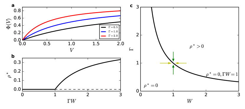
Figure 1: Firing function $\Phi(V)$, firing density and phase diagram for the static model. a, Rational firing function $\Phi(V)$ for $\Gamma=0.5$ (bottom), $1.0$ (middle) and $2.0$ (top). b, Firing density $\rho(\Gamma W)$. The absorbing state $\rho^{0}=0$ looses stability after $\Gamma W>\Gamma_{c}W_{c}=1$. c, Phase diagram in the $\Gamma\times W$ plane. An aSOC network can be created by adapting synapses (horizontal arrows) or adapting neuronal gains (vertical arrows) toward the critical line.

2.1 Stochastic neurons model with dynamic synapses

Adaptive SOC models try to turn the critical point into an attractive fixed point of some homeostatic dynamics. For example, in the LHG model, the spike of the presynaptic neuron produces depression of the synapse, which recovers within some large time scale [36, 4].

A model with stochastic neurons and LHG synapses uses the same equations (1 and 2),but now the synapses change with time [7]:

$$W_{ij}[t+1]=W_{ij}[t]+\frac{\Delta t}{\tau}\left(A-W_{ij}[t]\right)-uW_{ij}[t]X_{j}[t]\>.$$ (6)

Here, $\tau$ is the recovery time toward a baseline level $A$ and $0<u<1$ is the fraction of synaptic strength that is lost when the presynaptic neuron fires ($X_{j}=1$). From now, we always use $\Delta t=1$ ms, the typical width of a spike.

2.2 Stochastic neurons model with dynamic neuronal gains

Instead of adapting synapses toward the critical line $W_{c}=1/\Gamma$, we can adapt the gains toward the critical condition $\Gamma_{c}=1/W$, see Fig. 1c. This can be modeled as individual dynamic neuronal gains $\Gamma_{i}[t]$ ($i=1,\ldots,N$) that decrease by a factor $u$ if the neuron fires (diminishing the probability of subsequent firings) with a recovery time $1/\tau$ toward a baseline level $A$ [7]:

$$\Gamma_{i}[t+1]=\Gamma_{i}[t]+\frac{1}{\tau}\left(A-\Gamma_{i}[t]\right)-u\Gamma[t]X_{i}[t]\>,$$ (7)

which is very similar to the LHG dynamics. Notice, however, that here we have only $N$ equations for the neuronal gains instead of $N(N-1)$ equations for dynamic synapses, which allows the simulation of much larger systems. Also, the neuronal gain depression occurs due to the firing of the neuron $i$ (that is, $X_{i}[t]=1$) instead of the firing of the presynaptic neuron $j$. The biological location is also different: adaption of neuronal gains (that produces firing rate adaptation) is a process that occurs at the axonal initial segment (AIS) [33, 49] instead of dendritic synapses.

Like the LHG model, this dynamics inconveniently has three parameters ($\tau,A$ and $u$). Recently, we proposed a simpler dynamics with only one parameter [16, 15]:

$$\Gamma_{i}[t+1]=\Gamma_{i}[t]+\frac{1}{\tau}\Gamma_{i}[t]-\Gamma_{i}[t]X_{i}[t]=\left(1+\frac{1}{\tau}-X_{i}[t]\right)\Gamma_{i}[t]\>.$$ (8)

Averaging over the sites, we obtain the 2d MF map:

$$\rho[t+1] = \frac{\Gamma[t]W\rho[t](1-\rho[t])}{1+\Gamma[t]W\rho[t]}\>,$$ (9)

$$\Gamma[t+1] = \left(1+\frac{1}{\tau}-\rho[t]\right)\Gamma[t]\>.$$ (10)

2.3 Stability analysis for stochastic neurons with simplified neuronal gains

This case with a single-parameter dynamics ($\tau$) for the neuronal gains has the simplest analytic results, so it will be presented first and with more detail. For finite $\tau$, $\rho^{0}=0$ is no longer a solution, see equation (10), and the 2d map has a single fixed point $(\rho^{*},\Gamma^{*})$:

$$\rho^{*}=\frac{1}{\tau}\>,\>\>\>\>\>\>\>\>\>\>\>\>\>\>\>\>\>\Gamma^{*}=\frac{\Gamma_{c}}{1-2/\tau}\>,$$ (11)

where $\Gamma_{c}=1/W$. The relation between $\rho^{*}$ and $\Gamma^{*}$ is:

$$\rho^{*}=\frac{\Gamma^{*}W-1}{2\Gamma^{*}W}=\frac{\Gamma^{*}-\Gamma_{c}}{2\Gamma^{*}}\>,$$ (12)

which resembles the expression for the transcritical phase transition in the static system, see equation (5). Here, however, $\Gamma^{*}$ is no longer a parameter to be tuned but rather a fixed point of the 2d map to which the system dynamically converges. Notice that the critical point of the static model can be approximated for large $\tau$, with $(\rho^{*},\Gamma^{*})\rightarrow_{\tau\rightarrow\infty}(0,\Gamma_{c})$.

Performing a linear stability analysis of the fixed point (see Supplementary Information), we find that it corresponds to stable focus. The modulus of the complex eigenvalues is:

$$|\lambda^{\pm}|=\sqrt{1-\frac{\tau+2}{\tau(\tau-1)}}\>.$$ (13)

For large $\tau$ we have $|\lambda^{\pm}|=1-O(1/\tau)$, with a Neimark-Sacker-like critical point occurring when $|\lambda^{\pm}|=1$ where the focus turns out indifferent. For example, we have $|\lambda^{\pm}|\approx 0.990$ for $\tau=100$, $|\lambda^{\pm}|\approx 0.998$ for $\tau=500$ and $|\lambda^{\pm}|\approx 0.999$ for $\tau=1,000$. Since, due to biological motivations, $\tau$ is in the interval of $100-1000$ ms, we see that the focus is at the border of losing their stability. We call this point Neimark-Sacker-like because, in contrast to usual Neimark-Sacker one, the other side of the bifurcation, with $|\lambda^{\pm}|>1$, does not exist.

2.4 Finite size fluctuations produce stochastic oscillations

The stability of the fixed point focus is a result for the MF map that represents an infinite system without fluctuations. However, fluctuations are present in any finite size system and these fluctuations perturb the almost indifferent focus, exciting and sustaining stochastic oscillations that hover around the fixed point.

Without loss of generality, we fix $W=1$ in the simulations for the simple model with one parameter dynamics defined by Eq. (8). In Fig. 2a, we show the SO for the firing density $\rho[t]$ and average gain $\Gamma[t]$ ($\tau=500$ and $N=100,000$). As observed in the original LHG model [4], the stochastic oscillations have a sawtooth profile with no constant amplitude or period. In Fig. 2b, we show the SO in the phase plane $\rho$ vs $\Gamma$ for $\tau=100,500$ and $1,000$.

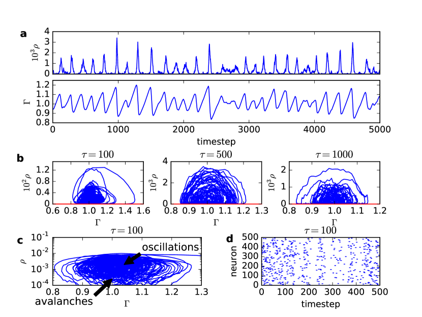
Figure 2: Stochastic neurons network with simplified (one parameter) neuronal gain dynamics (Eq. 8) and $W=1$. a, Stochastic oscillations for $\rho[t]$ and $\Gamma[t]$ ($\tau=500,N=100,000$ neurons). b, SO in the $\rho$ vs $\Gamma$ phase plane for $\tau=100,500$ and $1,000$ ($N=100,000$). c, SO in the log $\rho$ vs $\Gamma$ phase plane for $\tau=100$. d, Raster plot with $500$ neurons for $\tau=100$.

For small amplitude (harmonic) oscillations, the frequency is given by (see Supplementary Information):

$$\omega=\arctan\frac{\sqrt{\tau+2/\tau-4}}{\tau-2}\>.$$ (14)

The oscillation period, also for small amplitudes, is given by $T=2\pi/\omega$. The full oscillations are non-linear and their frequency and period depend on the amplitude.

Notice that, in the critical case, we have full critical slowing down: $\lim_{\tau\rightarrow\infty}\omega=\tau^{-1/2}\rightarrow 0,\lim_{\tau\rightarrow\infty}T\rightarrow\infty$. This means that, exactly at the critical point, the 2d map corresponds to a center without a period, and the SO would correspond to critical fluctuations similar to random walks in the $\rho$ vs $\Gamma$ plane. However, since for any physical/biological system the recovery time $\tau$ is finite, the critical point is not observable.

2.5 Stochastic oscillations and avalanches

For large $\tau$, part of the SO orbit occurs very close to the zero state $\rho^{0}=0$, see Figs. 2b-c. Due to finite-size fluctuations, the system frequently falls into this absorbing state. The orbits in phase space are interrupted. As in usual SOC simulations, we can define the size of an avalanche as the number $S$ of firing events between such zero states. After a zero state, we force a neuron to fire, to continue the dynamics, so that Figs. 2b-c are better understood as a series of patches (avalanches) terminating at $\rho[t]=0$, not as a single orbit.

The presence of the SO affects the distribution of avalanche sizes $P(S)$, see Fig. 3. For small $\tau$, $\rho^{*}$ is larger and it is more difficult for the SO to fall into the absorbing state. We observe a bump of very large avalanches (dragon king events). Increasing $\tau$, we move closer to the Neimark-Sacker-like critical point and observe power law avalanches with exponent $-3/2$ similar to those produced in the static model that suffers a transcritical bifurcation. So, by using a different mechanism (Neimar-Sacker-like versus transcritical bifurcation), our aSOC model can reproduce experimental data about power law neuronal avalanches [3, 12, 2, 13]. It also predicts that these avalanches can coexist with dragon kings events [44, 59]. We notice that Fig. 3 for $\tau=5000$ seems to be subcritical, but this is a finite-size effect [16]. The $P(S)$ distribution is not our main concern here and a more rigorous finite size analysis can be found in previous papers [7, 16].

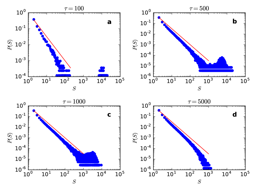
Figure 3: Avalanche size distribution $P(S)$ for the one parameter neuronal gain dynamics (Eq. 8) and $W=1$. a) $\tau=100$, b) $\tau=500$, c) $\tau=1,000$ and d) $\tau=5,000$; all plots have $N=100,000$. The straight line corresponds to the exponent $-3/2$. The apparent subcriticality in d) is a finite size effect.

2.6 Stochastic neurons with LHG dynamic gains

We now return to the case of dynamic gains with LHG dynamics, see equation (7). Without loss of generality, we use $W=1$, so that the static model has $\Gamma_{c}=1/W=1$. The map is given by:

$$\rho[t+1] = \frac{\Gamma[t]\rho[t](1-\rho[t])}{1+\Gamma[t]\rho[t]}\>,$$ (15)

$$\Gamma[t+1] = \Gamma[t]+\frac{1}{\tau}\left(A-\Gamma[t]\right)-u\Gamma[t]\rho[t]\>.$$ (16)

The trivial absorbing fixed point is $(\rho^{0},\Gamma^{0})=(0,A)$, stable for $A<1$, see Supplementary Material. For $A>1$, we have a non-trivial fixed point given by:

$$\rho^{*} = \frac{A-1}{2A+\tau u}\>,$$ (17)

$$\Gamma^{*} = \frac{2A+\tau u}{2+\tau u}=\Gamma_{c}+\frac{2(A-1)+\tau u}{2+\tau u}\>.$$ (18)

There is a relation between $\rho^{*}$ and $\Gamma^{*}$ that resembles the relation between the order parameter and the control parameter in the static model:

$$\rho^{*}=\frac{\Gamma^{*}-1}{2\Gamma^{*}}\>,$$ (19)

valid for $\Gamma^{*}>\Gamma_{c}=1$. Here, however, $\Gamma^{*}$ is a self-organized variable, not a control parameter to be finely tuned.

We notice that to set by hand $A=1$, pulling all gains toward $\Gamma_{i}=1$, produces the critical point $(\rho^{*},\Gamma^{*})=(0,1)$. Nevertheless, this is a fine tune that should not be allowed for SOC systems. We must use $A>1$, and reach the critical region only at the large $\tau$ limit: $\rho^{*}\approx(A-1)/\tau u$ and $\Gamma^{*}\approx\Gamma_{c}+2(A-1)/\tau u$.

Proceeding with the linear stability analysis, we obtain (see Supplementary Information):

$$\lambda^{+}\lambda^{-}=\left(1-\frac{1}{\tau}\right)\left(1-\frac{2(A-1)}{A+u\tau+1}\right)+\frac{u(A-1)^{2}}{(A+u\tau+1)(2A+u\tau)}\>.$$ (20)

To first order in $\tau$, we have:

$$\left|\lambda^{\pm}\right|=\sqrt{\lambda^{+}\lambda^{-}}=1-\frac{2(A-1)+u}{2u\tau}+O(\tau^{-2})\>,$$ (21)

which means that, for large $\tau$, the map is very close to the Neimark-Sacker-like critical point. As the stable focus approaches the critical value, the system exhibits oscillations as it approaches the fixed point due to demographic noise, leading to SO in finite-sized systems.

For example, with the typical values $A=1.05$ and $u=0.1$ [14, 9], we have $\left|\lambda^{\pm}\right|\approx 1-1/\tau$, which gives $\left|\lambda^{\pm}\right|\approx 0.990$ for $\tau=100$ and $\left|\lambda^{\pm}\right|\approx 0.999$ for $\tau=1,000$. In Fig. 4, we present the exact $\left|\lambda^{\pm}\right|$, the square root of equation (20), as a function of $\tau$ for several values of $A$ and $u$. For large $\tau,$ the frequency for harmonic oscillations is given by $\omega\simeq\sqrt{(A-1)/\tau}$ (see Supplementary Information).

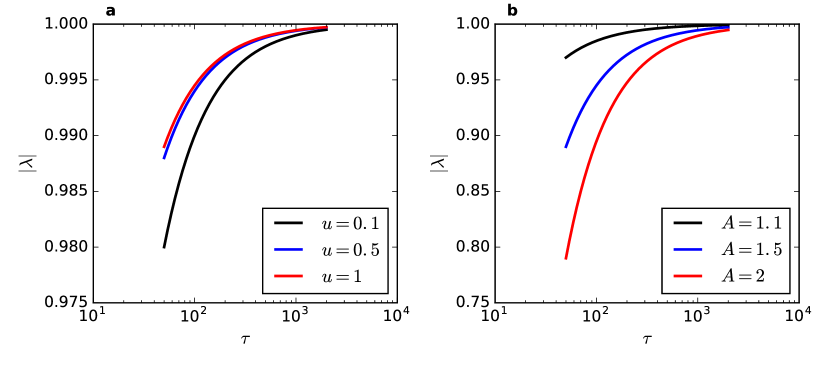
Figure 4: Modulus $|\lambda^{\pm}|$ as a function of $\tau$ for several values of $u$ and $A$. a, From top to bottom, $u=0.1,0.5$ and $1.0$, for $A=1.05$. b, From top to bottom, $A=1.1,1.5$ and $A=2.0$, for $u=0.1$.

The analysis of the stochastic neuron model with LHG synapses $W_{ij}[t]$, see equation (6), is very similar to the one above with LHG dynamic gains $\Gamma_{i}[t]$. The only difference is that we need to exchange $\Gamma$ by $W$. The eigenvalue modulus is the same, so that LHG dynamic synapses also produce SO. But, instead of presenting simulations in our complete graph system, which would involve $N(N-1)$ dynamic equations for the synapses, we prefer to discuss the LHG synapses for another system well known in the literature. We will also examine how SO depends on the system size $N$.

3 Excitable cellular automata with LHG synapses

We now consider an aSOC version of a probabilistic cellular automata well studied in the literature [31, 35, 46, 42, 57, 60]. It is a model for excitable media that yields a natural interpretation in terms of neuronal networks. Each site has $n$ states, $X=0$ (silent), $X=1$ (firing), $X=2,\ldots,n-1$ (refractory). Here we will use $n=2$.

Each neuron $i=1,\ldots,N$ has $K_{i}$ random neighbours (the average number in the network is $K=\left\langle K_{i}\right\rangle$) coupled by probabilistic synapses $P_{ij}\in[0,1]$ (here we use $K=10$, for implementation details see [31, 14, 9]). If the presynaptic neuron $j$ fires at time $t$, with probability $P_{ij}$ the postsynaptic neuron $i$ fires at $t+1$. The update is done in parallel, so the synapses are multiplicative, not additive like in the stochastic neuron model. All neurons that fire go to silence in the next step. Only neurons in the silent state can be induced to fire. Since $1-P_{ij}X_{j}$ is the probability that neighbour $j$ does not induces the firing of neuron $i$, we can write the update rule as:

$$P(X_{i}[t+1]=1)=(1-X_{i}[t])\left[1-\prod_{j}^{K_{i}}(1-P_{ij}X_{j})\right]\>,$$ (22)

The control parameter of the static model is the branching ratio $\sigma=K\left\langle P_{ij}\right\rangle$ and the critical value is $\sigma_{c}=1$.

In the cellular automata (CA) model with LHG synapses, we have [14, 9]:

$$P_{ij}[t+1]=P_{ij}[t]+\frac{1}{\tau}\left(\frac{A}{K}-P_{ij}[t]\right)-uP_{ij}[t]X_{j}[t]\>.$$ (23)

3.1 Mean field stability analysis

The 2d MF map close to the stationary state is:

$$\rho[t+1] = (1-\rho[t])\left[1-\left(1-\frac{\sigma[t]\rho[t]}{K}\right)^{K}\right]\>,$$ (24)

$$\sigma[t+1] = \sigma[t]+\frac{1}{\tau}\left(A-\sigma[t]\right)-u\sigma[t]\rho[t]\>,$$ (25)

where in the second line we multiplied equation (23) by $K$ and averaged over the synapses.

There is a trivial absorbing fixed point $(\rho^{0},\sigma^{0})=(0,A)$, stable up to $A=1$, see Supplementary Material. For $A>1$, there exists a single stable fixed point given implicitly by:

$$\rho^{*} = \left(1-\rho^{*}\right)\bigg{[}1-\bigg{(}1-\frac{A\rho^{*}}{(1+u\tau\rho^{*})K}\bigg{)}^{K}\bigg{]}\>,$$ (26)

$$\sigma^{*} = \frac{A}{1+u\tau\rho^{*}}\>,$$ (27)

which we can find numerically.

For this model we have numerical but no analytic results. However, we can find an approximate solution close to criticality, where $\rho^{*}$ is small (see Supplementary Information). Expanding in powers of $1/\tau$, we get:

$$|\lambda^{\pm}|=1-\left(\frac{(A-1)(2K-1)}{2uK}+\frac{1}{2}\right)\>\frac{1}{\tau}+O(\tau^{-2}).$$ (28)

This confirms that the same scenario of a weakly stable focus appears in the CA model.

This last result is particularly interesting. If we put $K=N-1$, the CA network becomes a complete graph. Performing the limit $N\rightarrow\infty$, equation (28) gives:

$$|\lambda^{\pm}|=1-\frac{A-1+u/2}{u\tau}+O(\tau^{-2})\>,$$ (29)

which is identical to the $\left|\lambda^{\pm}\right|$ value for the LHG stochastic neuron model, see equation (21).

Concerning the simulations, we must make a technical observation. In contrast to the static model [31], the relevant indicator of criticality here is no longer the branching ratio $\sigma$, but the principal eigenvalue $\Lambda\neq\sigma$ of the synaptic matrix $P_{ij}$, with $\Lambda_{c}=1$ [35, 57]. This occurs because the synaptic dynamics creates correlations in the random neighbour network [9]. So, the MF analysis, where correlations are disregarded, does not furnish the exact $\sigma$ or $\Lambda$ of the CA model. But there exists an annealed version of the model in which $\sigma^{*}=\Lambda^{*}$ and the MF analysis fully holds [14, 9].

In this annealed version, when some neuron fires, the depressing term $-uP_{ij}$ is applied to $K$ synapses randomly chosen in the network. This is not biologically realistic, but destroys correlations and restores the MF character of the model. Since all our analyses are done at the MF level, we prefer to present the simulation results using the annealed model. Concerning the SO phenomenology, there is no qualitative difference between the annealed and the original model defined by Eq. (23).

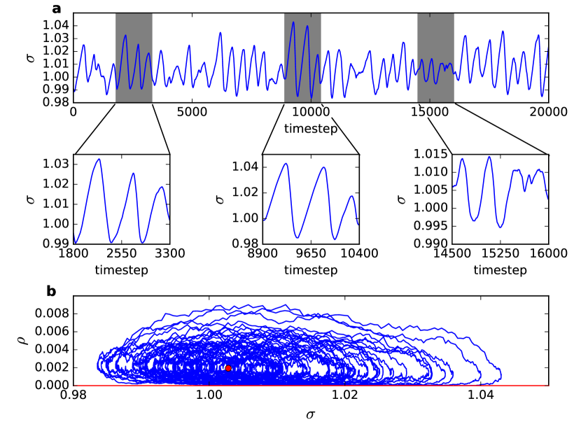
Figure 5: Stochastic oscillations for the annealed CA model with LHG synapses. a, The SO for $\sigma[t]$ has a sawtooth profile where large amplitudes have low frequency ($N=128,000$ neurons, $\tau=500$, $A=1.1$ and $u=0.1$). b, The SO in the phase plane $\rho$ vs $\sigma$. The red bullet is the fixed point given by Eqs. (26) and˜(27).

The full stochastic oscillations in a system with $N=128,000$ neurons and $\tau=500$ can be seen in Fig. 5a and b. The angular frequency for small amplitude oscillations is given by equation (92) (see Supplementary Information). We have $\omega\simeq\sqrt{(A-1)/\tau}$ for large $\tau$, which is the same behavior found for stochastic neurons. The power spectrum of the time evolution of $\rho$ and $\sigma$ is shown in Fig. 6. The peak frequency gets closer to the theoretical $\omega$ (vertical line) for larger system sizes because the oscillations have smaller amplitudes, going to the small oscillations limit.

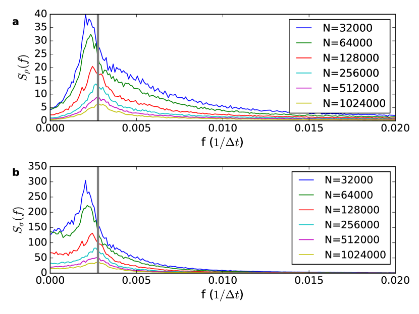
Figure 6: Power spectrum of the time evolution of $\rho$ and $\sigma$ in the annealed CA model with LHG synapses. a and b, power spectrum of the time evolution of $\rho$ and $\sigma$, respectively, for different system sizes ($\tau=320$, $A=1.1$, $u=0.1$). The vertical lines mark the theoretical value of the frequency of small oscillations of the evolution of the MF map near the fixed point calculated from Eq. (92).

3.2 Dependence of the stochastic oscillations on system size

Now we ask if the SO survive in the thermodynamic limit. In principle, given that fluctuations vanish in this limit, and we have always damped focus for finite $\tau$, the SO should also disappear when $1/N\rightarrow 0$. In contrast, Bonachela et al. claimed that, in the LHG model, the amplitude of the oscillations basically does not change with $N$ and is non-zero in the thermodynamic limit [4]. Indeed, they proposed that this feature is a core ingredient of SOqC.

In Fig. 7, we measured the average $\left\langle\sigma[t]\right\rangle$ and the standard deviation $\Delta\sigma$ of the $\sigma[t]$ time series of the annealed model. We used $\tau=320,500,1,000$ and $2,000$ and system sizes from $N=4,000$ to $1,024,000$. We interpret our findings as a $\tau$ dependent crossover phenomenon due to a trade-off between the level of fluctuations (which depends on $N$) and the level of dampening (which depends on $\tau$): for a given $\tau$, a small $N$ can produce sufficient fluctuations so that the SO are sustained without change of $\Delta\sigma$. Nonetheless, starting from some $N(\tau)$, the fluctuations are not sufficient to compensate the dampening given by $|\lambda^{\pm}|<1$ and $\Delta\sigma$ starts to decrease for increasing $N$. The larger the $\tau$, the less damped is the focus and the SO survive without change to a larger $N$ (the plateau in Fig. 7b is more extended to the left).

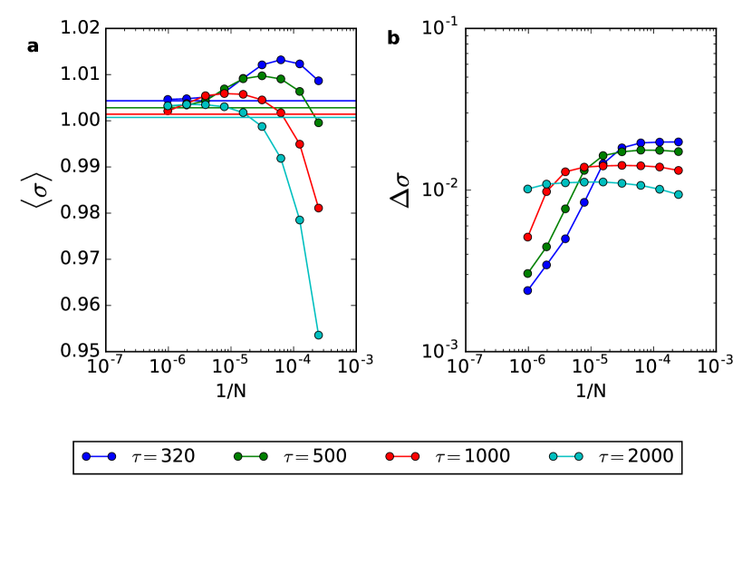
Figure 7: Average and standard deviation of the SO time series (CA model) as a function of $1/N$. a, Average $\left\langle\sigma[t]\right\rangle$ for different $\tau$ values. Horizontal lines are the value of the fixed points $\sigma^{*}$ given by equation (27). b, Standard deviation $\Delta\sigma$ for different $\tau$ values. Parameters are $A=1.1$ and $u=0.1$. All measures are taken in a window of $10^{6}$ time steps after discarding transients.

So, the conclusion is that, for any finite $\tau$, the SO do not survive up to the thermodynamic limit, although they can be observed in very large systems. This is compatible with Fig. 6 where the power spectrum decreases with $N$. We also see in Fig. 7a that $\left\langle\sigma[t]\right\rangle\rightarrow\sigma^{*}$ for increasing $N$, so the system settles without variance at the MF fixed point $(\rho^{*},\sigma^{*})$ in the infinite size limit.

We can reconcile our findings with those of the LHG model [36, 4] remembering an important technical detail: these authors used a synaptic dynamics with $\tau=\tau_{0}N$, in an attempt to have the fixed point converging to the critical one in the thermodynamic limit (the same scaling is used in other models [23, 14]). In systems with this scaling, the fluctuations decay with $N$ but, at the same time, the dampening controlled by $\lambda(\tau(N))$ also decays with $N$. For this scaling, we can accord that the SO survive in the thermodynamic limit. However, we already emphasized that this is a non-biological and non-local scaling choice [9, 7, 16] because the recovery time $\tau$ must be finite and the knowledge of the network size $N$ is non-local.

However, from a biological point of view, this discussion is not so relevant: although the finite-size fluctuations (called demographic noise in the literature [38, 51, 11, 45]) disappear for large $N$, external (environmental) noise of biological origin, not included in the models, never vanishes in the thermodynamic limit. So, for practical purposes, the SO and the associated dragon kings would always be present in more realistic noisy networks and experiments.

4 Discussion and Conclusion

We now must stress what is new in our findings. Standard SOC models are related to static systems presenting an absorbing state phase transition [22, 30, 21, 50]. At the MF level, these static systems are described by an 1d map $\rho[t+1]=F(\rho[t])$ for the density of active sites, and the phase transition corresponds to a transcritical bifurcation where the critical point is an indifferent node. This indifferent equilibrium enables the occurrence of scale-invariant fluctuations in the $\rho[t]$ variable, that is, scale-invariant avalanches but not stochastic oscillations.

In aSOC networks, the original control parameter of the static system turns out an activity dependent variable leading to 2d MF maps. We performed a MF fixed point stability analysis for three systems: 1) a stochastic neuronal model with one-parameter neuronal gain dynamics, 2) the same model with LHG gain dynamics, and 3) the CA model with LHG synapses. For the first one we obtained very simple and transparent analytic results; for the LHG dynamics we also got analytic, although more complex, results; finally, for the CA model, we were able to obtain a first order approximation for large recovery time $\tau$. Curiously, in the limit of $K=(N-1)\rightarrow\infty$ neighbours, the stochastic neuron model and the CA model have exactly the same first order leading term. The complex eigenvalues have modulus $|\lambda^{\pm}|\approx 1-O(1/\tau)$ and, for large $\tau$, the fixed point is a focus at the border of indifference. This means that, in finite size systems, the dampening is very low and fluctuations can excite and sustain stochastic oscillations.

About the generality of our results, we conjecture they are generic and valid for the whole class of aSOC models, from networks with discrete deletion-recovery of links [39, 40, 23] to continuous depressing-recovering synapses [36, 4, 14, 9] and neurons with firing rate adaptation [7, 16, 15]). At the mean-field level, all of them are described by similar two-dimensional dynamical systems: one variable for the order parameter, another for the adaptive mechanism. For example, the prototypical LHG model [36, 4] uses continuous time LIF neurons (which is equivalent to setting $\Gamma\rightarrow\infty$ and $\theta,\mu>0$ in our model). Although with more involved calculations, in principle one could do a similar mean-field calculation and obtain a 2d dynamical system with an almost unstable focus close to criticality, explaining the SO observed in that model. In another aspect of generality, stochastic oscillations have been observed previously in other SOqC systems (forest-fire models [29, 55] and some special sandpile models [20, 52]) that share a similar MF description with aSOC systems. Indeed, it seems that stochastic oscillations is a distinctive feature of self-organized quasi-criticality, as defined by Bonachela et al. [5, 4].

We also emphasize that the fact that our network has only excitatory neurons is not a limitation of this study. In a future work [32], we will show that our model can be fully generalized to an excitatory-inhibitory network very similar to the Brunel model [8], with the same results.

So, it must be clear that what is new here is not the stochastic oscillations (quasicycles) in biosystems, since there is a whole literature about that [43, 38, 51, 56, 1, 11, 45]. What is new here is the interaction of the SO with a critical point with an absorbing state. This interaction interrupts the oscillations, producing the phenomenology of avalanches and dragon kings. This is our novel proposal for a mechanism that produces dragon kings coexisting with limited power law avalanches.

In conclusion, contrasting to standard SOC, aSOC systems present stochastic oscillations that will not vanish in the thermodynamic limit if external (environmental) noise is present. But what seems to be a shortcoming for neural aSOC models could turn out to be an advantage. Since the adaptive dynamics with large $\tau$ has good biological motivation, it is possible that SO are experimentally observable, providing new physics beyond the standard model for SOC. The presence of the Neimark-Sacker-like bifurcation affects the distribution of avalanche sizes $P(S)$, creates dragon king events, and all this phenomenology can be measured [17, 48, 47]. In particular, our raster plots results are compatible with system-sized events (synchronized fires) recently observed in neuronal cultures [44, 59]. So, we have experimental predictions that differ from standard SOC based on a transcritical bifurcation (and also from criticality models with Griffiths phases [41, 28]). We propose that the experimental detection of stochastic oscillations and dragon-kings should be the next experimental challenge in the field of neuronal avalanches.

Finally, we speculate that non-mean field models (square or cubic lattices) with dynamic gains and SO could be applied to the modeling of dragon-kings (large quasiperiodic ”characteristic”) earthquakes that coexist with power-law Gutemberg-Richter distributions for the small events [10, 58]. This will be pursued in another work.

Methods

Numerical Calculations: Numerical calculations were done by using MATLAB softwares. Simulation procedures: Simulation codes were made in Fortran90 and C++11.

Author contributions

AAC and JGFC performed the simulations and prepared all the figures. JGFC, LB, MC and OK made the analytic calculations. All authors contributed to the writing of the manuscript.

Competing interests

The authors declare that they have no competing financial interests.

Supplementary Information

Stability analysis of the stochastic neuron model with one parameter ($\tau$) gain dynamics

The MF map is:

$$\rho[t+1] = \frac{\Gamma[t]W\rho[t](1-\rho[t])}{1+\Gamma[t]W\rho[t]}=F(\rho[t],\Gamma[t])\>,$$ (30)

$$\Gamma[t+1] = \left(1+\frac{1}{\tau}-\rho[t]\right)\Gamma[t]=G(\rho[t],\Gamma[t])\>.$$ (31)

Notice that $(\rho^{0}=0,\Gamma)$ is not a fixed point. The single fixed point is:

$$\rho^{*}=\frac{1}{\tau}\>,\>\>\>\>\>\>\>\>\>\>\>\>\>\>\>\>\>\Gamma^{*}=\frac{\Gamma_{c}}{1-2/\tau}\>.$$ (32)

To perform the fixed point stability analysis we calculate partial derivatives evaluated at the fixed point (denoted by $\left.\right]_{*}$):

$$a=\left.\frac{\partial F}{\partial\rho}\right]_{*} = \frac{\Gamma^{*}W-2\Gamma^{*}W\rho^{*}-(\Gamma^{*}W\rho^{*})^{2}}{\left[1+\Gamma^{*}W\rho^{*}\right]^{2}}=\frac{\tau-3}{\tau-1}\>,$$ (33)

$$b=\left.\frac{\partial F}{\partial\Gamma}\right]_{*} = \frac{W\rho^{*}(1-\rho^{*})}{\left[1+\Gamma^{*}W\rho^{*}\right]^{2}}=\frac{W(\tau-2)^{2}}{\tau^{2}(\tau-1)}\>,$$ (34)

$$c=\left.\frac{\partial G}{\partial\rho}\right]_{*} = -\Gamma^{*}=-\frac{\tau}{W(\tau-2)}\>,$$ (35)

$$d=\left.\frac{\partial G}{\partial\Gamma}\right]_{*} = 1+1/\tau-\rho^{*}=1\>.$$ (36)

The eigenvalues of the system Jacobian matrix at the fixed point $(\rho^{*},\Gamma^{*})$ are determined by

$$\det(J-\lambda I)=(a-\lambda)(d-\lambda)-bc=0\>.$$ (37)

So, the characteristic equation is:

$$\lambda^{2}-\left[\left(\frac{\tau-3}{\tau-1}\right)+1\right]\lambda+\frac{\tau-3}{\tau-1}+\frac{\tau-2}{\tau(\tau-1)}=0\>.$$ (38)

That can be written as:

$$\tau(\tau-1)\lambda^{2}-(2\tau^{2}-4\tau)\lambda+\tau^{2}-2\tau-2=0\>,$$ (39)

with solutions:

$$\lambda^{\pm} = \frac{\tau^{2}-2\tau\pm\sqrt{\Delta}}{\tau(\tau-1)}\>,$$ (40)

$$\Delta = (\tau^{2}-2\tau)^{2}-\tau(\tau-1)(\tau^{2}-2\tau-2)$$ (41)

This equation has no meaning for $\tau<2$ since this would give $\rho^{*}=1/\tau>1/2$. When $2<\tau<2+\sqrt{2}$ we have $\Delta>0$, $\lambda$ real and $|\lambda|<1$, that is, the fixed point $(\rho^{*},\Gamma^{*})$ is a stable node. However, when $\tau>2+\sqrt{2}=3.4142\ldots$, we have $\Delta<1$ and two complex roots $\lambda^{\pm}$ with $|\lambda|=\sqrt{\lambda^{+}\lambda^{-}}<1$, that is, we have a stable focus with:

$$\lambda^{\pm} = \frac{\tau^{2}-2\tau\pm i\sqrt{-\Delta}}{\tau(\tau-1)}\>,$$ (42)

$$|\lambda^{\pm}| = \sqrt{\lambda^{+}\lambda^{-}}=\sqrt{\frac{\tau^{2}-2\tau-2}{\tau(\tau-1)}}=\sqrt{1-\frac{\tau+2}{\tau(\tau-1)}}\>,$$ (43)

which leads to equation (13).

For small amplitude (harmonic) oscillations, the frequency is given by the angle of the eigenvalues written in polar coordinates. We can write it in terms of the determinant $D$ and trace $T$ of the Jacobian matrix $J$ as

$$\omega \equiv |\omega^{\pm}|=\arctan{\sqrt{\frac{4D}{T^{2}}-1}}=\arctan\frac{\sqrt{\tau+2/\tau-4}}{\tau-2}$$ (44)

When $\tau\rightarrow\infty$,

$$\omega\simeq\sqrt{\frac{1}{\tau}}$$ (45)

Stability analysis of the stochastic neuron model with LHG gain dynamics

The MF map is given by:

$$\rho[t+1] = \frac{\Gamma[t]\rho[t](1-\rho[t])}{1+\Gamma[t]\rho[t]}=F(\rho[t],\Gamma[t])\>,$$ (46)

$$\Gamma[t+1] = \Gamma[t]+\frac{1}{\tau}\left(A-\Gamma[t]\right)-u\Gamma[t]\rho[t]=G(\rho[t],\Gamma[t])\>.$$ (47)

We have two fixed points. The absorbing state fixed point:

$$\rho^{0}=0\>\>\>\>\>\>\>\>\>\>\>\>\>\>\>\>\>\>\>\>\>\>\>\Gamma^{0}=A\>,$$ (48)

and the non trivial fixed point $(\rho^{*},\Gamma^{*})$:

$$\rho^{*}=\frac{A-1}{2A+\tau u}\>,\>\>\>\>\>\>\>\>\>\>\>\>\>\>\Gamma^{*}=\frac{2A+\tau u}{2+\tau u}\>.$$ (49)

Partial derivatives of $F$ and $G$ with respect to $\rho$ and $\Gamma$ are:

$$\frac{\partial F(\rho,\Gamma)}{\partial\rho} = -\frac{\Gamma\left(2\rho+\rho^{2}\Gamma-1\right)}{(\rho\Gamma+1)^{2}}\>,$$ (50)

$$\frac{\partial F(\rho,\Gamma)}{\partial\Gamma} = -\frac{(\rho-1)\rho}{(\rho\Gamma+1)^{2}}\>,$$ (51)

$$\frac{\partial G(\rho,\Gamma)}{\partial\rho} = -\Gamma u\>,$$ (52)

$$\frac{\partial G(\rho,\Gamma)}{\partial\Gamma} = -\frac{1}{\tau}-u\rho+1\>.$$ (53)

Evaluating at the trivial fixed point, we get:

$$a = \left.\frac{\partial F}{\partial\rho}\right]_{0}=\Gamma=A\>,$$ (54)

$$b = \left.\frac{\partial F}{\partial\Gamma}\right]_{0}=0\;,$$ (55)

$$c = \left.\frac{\partial G}{\partial\rho}\right]_{0}=-u\Gamma=-uA\>,$$ (56)

$$d = \left.\frac{\partial G}{\partial\Gamma}\right]_{0}=1-\frac{1}{\tau}\>.$$ (57)

The eigenvalues are found from $(a-\lambda)(d-\lambda)-bc=0$, or:

$$(A-\lambda)(1-1/\tau-\lambda) = 0\>,$$ (58)

$$\lambda^{2}-(A+1-1/\tau)\lambda+(1-1/\tau)A = 0\>,$$ (59)

with solution:

$$\lambda^{\pm} = \frac{(A+1-1/\tau)\pm\sqrt{\Delta}}{2}\>,$$ (60)

$$\Delta = (A+1-1/\tau)^{2}-4(1-1/\tau)A=[A-(1-1/\tau)]^{2}\>.$$ (61)

Notice that $\Delta\geq 0$ so the eigenvalues are always real: the fixed point is an attractive or repulsive node. The final solution of Eq. 60 is:

$$\lambda^{+} = A\>,$$ (62)

$$\lambda^{-} = 1-1/\tau\>.$$ (63)

This means that the fixed point $(\rho^{0}=0,\Gamma^{0}=A)$ is stable for $\lambda^{+}=A<1$. The critical point is $A=1$.

This analysis show that we can have a subcritical state $(0,A)$, an attractive node, if we use $A<1$. On the other hand, if we use $A>1$, the absorbing state looses its stability and the non trivial fixed point $(\rho^{*},\Gamma^{*})$ is the unique stable solution. For $A=1$, the point $(\rho^{0}=0,\Gamma^{0}=1)$ is an indifferent node.

Evaluating the derivatives at the non trivial fixed point, we get:

$$\left.\frac{\partial F}{\partial\rho}\right]_{*} = \frac{3-A+u\tau}{A+u\tau+1}\>,$$ (64)

$$\left.\frac{\partial F}{\partial\Gamma}\right]_{*} = \frac{(A-1)(2+u\tau)^{2}}{(A+u\tau+1)(2A+u\tau)^{2}}\>,$$ (65)

$$\left.\frac{\partial G}{\partial\rho}\right]_{*} = -\frac{u(2A+u\tau)}{2+u\tau}\>,$$ (66)

$$\left.\frac{\partial G}{\partial\Gamma}\right]_{*} = 1-\frac{1}{\tau}-\frac{u(A-1)}{2A+u\tau}\>,$$ (67)

As before, the eigenvalues of the Jacobian matrix at the fixed point $(\rho^{*},\Gamma^{*})$ are determined by equation (37). After some algebra, we get:

$$|\lambda^{+}\lambda^{-}| = ad-bc$$ (68)

$$= \frac{(1-1/\tau-\frac{u(A-1)}{2A+u\tau})(3-A+u\tau)}{(A+u\tau+1)}+\frac{u(2+u\tau)(A-1)}{(2A+u\tau)(A+u\tau+1)}\>,$$

$$= \left(1-\frac{1}{\tau}\right)\left(1-\frac{2(A-1)}{A+u\tau+1}\right)+\frac{u(A-1)^{2}}{(A+u\tau+1)(2A+u\tau)}\>.$$

For large $\tau$, we have:

$$\left|\lambda^{\pm}\right|=\sqrt{\lambda^{+}\lambda^{-}}=1-\frac{2(A-1)+u}{2u\tau}+O(\tau^{-2})\>,$$ (69)

which means that, for large $\tau$, the map is very close to a Neimark-Sacker-like critical point. As before, the focus can be excited by fluctuations, generating the SO.

The frequency for small amplitude oscillations is $\omega\equiv|\omega^{\pm}|=\arctan{\sqrt{\frac{4D}{T^{2}}-1}}$, where $D$ and $T$ are respectively the determinant and trace of the Jacobian matrix. When $\tau\rightarrow\infty$,

$$\omega\simeq\sqrt{\frac{A-1}{\tau}}$$ (70)

which is similar to the $\tau^{-1/2}$ behavior of the simple gain dynamics, Eq. (45).

Stability analysis of the Cellular Automata model with LHG synapses

The 2d MF map near the stationary state is:

$$\rho[t+1] = (1-\rho[t])\left[1-\left(1-\frac{\sigma[t]\rho[t]}{K}\right)^{K}\right]=F(\rho[t],\sigma[t])\>,$$ (71)

$$\sigma[t+1] = \sigma[t]+\frac{1}{\tau}\left(A-\sigma[t]\right)-u\sigma[t]\rho[t]=G(\rho[t],\sigma[t])\>,$$ (72)

where in the second line we multiplied equation (23) by $K$ and averaged over the synapses. As before, the stability of the map is given by the eigenvalues of the Jacobian matrix $J(\rho,\sigma)$ at the fixed points. The matrix elements are:

$$\left.\frac{\partial F}{\partial\rho}\right] = \bigg{[}\bigg{(}1-\frac{\sigma\rho}{K}\bigg{)}^{K}-1\bigg{]}+(1-\rho)\sigma\bigg{(}1-\frac{\sigma\rho}{K}\bigg{)}^{K-1}\>,$$ (73)

$$\left.\frac{\partial F}{\partial\sigma}\right] = (1-\rho)\rho\bigg{(}1-\frac{\rho\sigma}{K}\bigg{)}^{K-1}\>,$$ (74)

$$\left.\frac{\partial G}{\partial\rho}\right] = -u\sigma\>,$$ (75)

$$\left.\frac{\partial G}{\partial\sigma}\right] = 1-\frac{1}{\tau}-u\rho\>.$$ (76)

Thus, we can plug in the solutions of equations (26) and (26) in equations (73-76) and find the eigenvalues of $J(\rho,\sigma)$.

Similarly to the previous model, the MF map of the CA with LHG synapses has two fixed points. The first one is the absorbing state fixed point and is given by

$$\rho^{0}=0\>\>\>\>\>\>\>\>\>\>\>\>\>\>\>\>\>\>\>\>\>\>\>\sigma^{0}=A\>.$$ (77)

The second one is nontrivial and must be solved numerically.

We can compute the elements of the Jacobian matrix at the absorbing state fixed point

$$\left.\frac{\partial F}{\partial\rho}\right]_{0} = A\>,$$ (78)

$$\left.\frac{\partial F}{\partial\sigma}\right]_{0} = 0\;,$$ (79)

$$\left.\frac{\partial G}{\partial\rho}\right]_{0} = -uA\>,$$ (80)

$$\left.\frac{\partial G}{\partial\sigma}\right]_{0} = 1-\frac{1}{\tau}\>,$$ (81)

which is the same result of Eqs. (54–57). This matrix has two eigenvalues: $1-1/\tau$ and $A$. The eigenvalue $1-\tau$ corresponds to the $\sigma$ axis, which is a stable direction. The eigenvalue $A$ corresponds to a unstable (stable) direction for $A>1$ $(A<1)$.

If we assume that we are close to criticality, where $\rho^{*}$ is small, we can find an approximate solution for $J(\rho,\sigma)$ at the nontrivial fixed point. Expanding the binomial in equation (24) to first order and solving for $\rho^{*}$, we find:

$$\rho* = \frac{A-1}{A+u\tau}\>,$$ (82)

$$\sigma^{*} = \frac{A+u\tau}{1+u\tau}=1+\frac{A-1}{1+u\tau}\>,$$ (83)

where we used equation (26) to compute $\sigma^{*}$. Note that, as before, this solution exists only if $A-1>0$. This is the exact condition to the absorbing state solution be unstable.

Inserting in equations (73-76), we have:

$$J=\left({\begin{array}[]{cc}1-a&b\\ -c&1-d\\ \end{array}}\right),$$ (84)

where

$$a = \frac{(2K-1)(A-1)}{K(1+u\tau)}\>,$$ (85)

$$b = \frac{A-1}{(A+u\tau)^{2}}\bigg{(}1+u\tau-\frac{(A-1)(K-1)}{K}\bigg{)}\>,$$ (86)

$$c = \frac{u(A+u\tau)}{1+u\tau}\>,$$ (87)

$$d = \frac{1}{\tau}+\frac{u(A-1)}{A+u\tau}\>.$$ (88)

Note that they are all positive quantities. The eigenvalues of $J$ are:

$$\lambda^{\pm}=1-\frac{a+d}{2}\pm\frac{1}{2}\sqrt{(a-d)^{2}-4bc}.$$ (89)

For systems to be close to criticality, we must have $\tau\gg 1$. Thus, $a$, $b$ and $d$ are of $O(1/\tau)$, while $c=O(1)$. Therefore, the $4bc$ term dominates the square root argument in equation (89). Hence, we have two complex conjugate eigenvalues with modulus and argument given by:

$$\left|\lambda^{\pm}\right|=\sqrt{1-(a+d)+da+bc}\>.$$ (90)

We can expand $|\lambda^{\pm}|$ in powers of $1/\tau$:

$$|\lambda^{\pm}|=1-\left(\frac{(A-1)(2K-1)}{2uK}+\frac{1}{2}\right)\>\frac{1}{\tau}+O(\tau^{-2}).$$ (91)

This confirms that the same scenario of weakly stable focus appears in the CA model. The harmonic frequency is:

$$\omega\equiv|\omega^{\pm}|=\arctan{\frac{\sqrt{4bc-(a-d)^{2}}}{2-(a+d)}}\>.$$ (92)

To first order in $\tau$, we get $\omega\simeq\sqrt{(A-1)/\tau}$, which shows that the frequency of oscillations is vanishingly small for large $\tau$, being identical to equation (70).

References

- [1] Peter H Baxendale and Priscilla E Greenwood. Sustained oscillations for density dependent markov processes. J. Math. Bio., 63(3):433–457, 2011.
- [2] John M Beggs. The criticality hypothesis: how local cortical networks might optimize information processing. Philos. Trans. R. Soc. A, 366(1864):329–343, 2008.
- [3] John M Beggs and Dietmar Plenz. Neuronal avalanches in neocortical circuits. J. Neurosci., 23(35):11167–11177, 2003.
- [4] Juan A Bonachela, Sebastiano de Franciscis, Joaquín J Torres, and Miguel A Muñoz. Self-organization without conservation: are neuronal avalanches generically critical? J. Stat. Mech. - Theory Exp., 2010(02):P02015, 2010.
- [5] Juan A Bonachela and Miguel A Muñoz. Self-organization without conservation: true or just apparent scale-invariance? J. Stat. Mech. - Theory Exp., 2009(09):P09009, 2009.
- [6] Stefan Bornholdt and Thimo Rohlf. Topological evolution of dynamical networks: global criticality from local dynamics. Phys. Rev. Lett., 84(26):6114, 2000.
- [7] Ludmila Brochini, Ariadne Andrade Costa, Miguel Abadi, Antônio C Roque, Jorge Stolfi, and Osame Kinouchi. Phase transitions and self-organized criticality in networks of stochastic spiking neurons. Sci. Rep., 6:35831, 2016.
- [8] Nicolas Brunel. Dynamics of sparsely connected networks of excitatory and inhibitory spiking neurons. Journal of Computational Neuroscience, 8(3):183–208, 2000.
- [9] J G F Campos, A A Costa, M Copelli, and O Kinouchi. Correlations induced by depressing synapses in critically self-organized networks with quenched dynamics. Phys. Rev. E, 95:042303, Apr 2017.
- [10] J M Carlson. Time intervals between characteristic earthquakes and correlations with smaller events: An analysis based on a mechanical model of a fault. J. Geophys. Res., 96(B3):4255–4267, 1991.
- [11] Joseph D Challenger, Duccio Fanelli, and Alan J McKane. The theory of individual based discrete-time processes. Journal of Statistical Physics, 156(1):131–155, 2014.
- [12] Dante R Chialvo. Critical brain networks. Physica A, 340(4):756–765, 2004.
- [13] Dante R Chialvo. Emergent complex neural dynamics. Nat. Phys., 6(10):744–750, 2010.
- [14] A A Costa, M Copelli, and O Kinouchi. Can dynamical synapses produce true self-organized criticality? J. Stat. Mech. - Theory Exp., 2015(6):P06004, 2015.
- [15] Ariadne A Costa, Mary Jean Amon, Olaf Sporns, and Luis H Favela. Fractal analyses of networks of integrate-and-fire stochastic spiking neurons. In International Workshop on Complex Networks, pages 161–171. Springer, 2018.
- [16] Ariadne A. Costa, Ludmila Brochini, and Osame Kinouchi. Self-organized supercriticality and oscillations in networks of stochastic spiking neurons. Entropy, 19(8):399, 2017.
- [17] L de Arcangelis. Are dragon-king neuronal avalanches dungeons for self-organized brain activity? Eur. Phys. J. Spec. Top., 205(1):243–257, 2012.
- [18] Lucilla de Arcangelis and Hans Herrmann. Activity-dependent neuronal model on complex networks. Front. Physiol., 3:62, 2012.
- [19] Lucilla de Arcangelis, Carla Perrone-Capano, and Hans J Herrmann. Self-organized criticality model for brain plasticity. Phys. Rev. Lett., 96(2):028107, 2006.
- [20] Serena di Santo, Raffaella Burioni, Alessandro Vezzani, and Miguel A Muñoz. Self-organized bistability associated with first-order phase transitions. Physical review letters, 116(24):240601, 2016.
- [21] Ronald Dickman, Miguel A Muñoz, Alessandro Vespignani, and Stefano Zapperi. Paths to self-organized criticality. Braz. J. Phys., 30(1):27–41, 2000.
- [22] Ronald Dickman, Alessandro Vespignani, and Stefano Zapperi. Self-organized criticality as an absorbing-state phase transition. Phys. Rev. E, 57(5):5095, 1998.
- [23] Felix Droste, Anne-Ly Do, and Thilo Gross. Analytical investigation of self-organized criticality in neural networks. J. R. Soc. Interface, 10(78):20120558, 2013.
- [24] Antonio Galves and Eva Löcherbach. Infinite systems of interacting chains with memory of variable length — a stochastic model for biological neural nets. J. Stat. Phys., 151(5):896–921, 2013.
- [25] Wulfram Gerstner. Associative memory in a network of biological neurons. In Advances in Neural Information Processing Systems, pages 84–90, 1991.
- [26] Wulfram Gerstner and Werner M Kistler. Spiking Neuron Models: Single Neurons, Populations, Plasticity. Cambridge Univ. Press, 2002.
- [27] Wulfram Gerstner and J Leo van Hemmen. Associative memory in a network of ‘spiking’ neurons. Network: Comput. Neural Syst., 3(2):139–164, 1992.
- [28] Mauricio Girardi-Schappo, Germano S Bortolotto, Jheniffer J Gonsalves, Leonel T Pinto, and Marcelo H R Tragtenberg. Griffiths phase and long-range correlations in a biologically motivated visual cortex model. Sci. Rep., 6:29561, 2016.
- [29] Peter Grassberger and Holger Kantz. On a forest fire model with supposed self-organized criticality. Journal of Statistical Physics, 63(3-4):685–700, 1991.
- [30] Henrik Jeldtoft Jensen. Self-organized Criticality: Emergent Complex Behavior in Physical and Biological Systems. Cambridge Univ. Press, Cambridge, UK, 1998.
- [31] Osame Kinouchi and Mauro Copelli. Optimal dynamical range of excitable networks at criticality. Nat. Phys., 2(5):348–351, 2006.
- [32] Osame Kinouchi, Ariadne de Andrade Costa, Ludmila Brochini, and Mauro Copelli. Unification between balanced networks and self-organized criticality models. preprint, 00(0):00, 2018.
- [33] Maarten H P Kole and Greg J Stuart. Signal processing in the axon initial segment. Neuron, 73(2):235–247, 2012.
- [34] Daniel B Larremore, Woodrow L Shew, Edward Ott, Francesco Sorrentino, and Juan G Restrepo. Inhibition causes ceaseless dynamics in networks of excitable nodes. Phys. Rev. Lett., 112(13):138103, 2014.
- [35] Daniel B Larremore, Woodrow L Shew, and Juan G Restrepo. Predicting criticality and dynamic range in complex networks: effects of topology. Phys. Rev. Lett., 106(5):058101, 2011.
- [36] Anna Levina, J Michael Herrmann, and Theo Geisel. Dynamical synapses causing self-organized criticality in neural networks. Nat. Phys., 3(12):857–860, 2007.
- [37] Anna Levina, J Michael Herrmann, and Theo Geisel. Phase transitions towards criticality in a neural system with adaptive interactions. Phys. Rev. Lett., 102(11):118110, 2009.
- [38] Alan J McKane and Timothy J Newman. Predator-prey cycles from resonant amplification of demographic stochasticity. Phys. Rev. Lett., 94(21):218102, 2005.
- [39] Christian Meisel and Thilo Gross. Adaptive self-organization in a realistic neural network model. Phys. Rev. E, 80(6):061917, 2009.
- [40] Christian Meisel, Alexander Storch, Susanne Hallmeyer-Elgner, Ed Bullmore, and Thilo Gross. Failure of adaptive self-organized criticality during epileptic seizure attacks. PLoS Comput. Biol., 8(1):e1002312, 2012.
- [41] Paolo Moretti and Miguel A Muñoz. Griffiths phases and the stretching of criticality in brain networks. Nat. Commun., 4:2521, 2013.
- [42] Thiago S Mosqueiro and Leonardo P Maia. Optimal channel efficiency in a sensory network. Phys. Rev. E, 88(1):012712, 2013.
- [43] R M Nisbet and W S C Gurney. A simple mechanism for population cycles. Nature, 263(5575):319–320, 1976.
- [44] Javier G Orlandi, Jordi Soriano, Enrique Alvarez-Lacalle, Sara Teller, and Jaume Casademunt. Noise focusing and the emergence of coherent activity in neuronal cultures. Nat. Phys., 9(9):582–590, 2013.
- [45] César Parra-Rojas, Joseph D Challenger, Duccio Fanelli, and Alan J McKane. Intrinsic noise and two-dimensional maps: Quasicycles, quasiperiodicity, and chaos. Physical Review E, 90(3):032135, 2014.
- [46] Sen Pei, Shaoting Tang, Shu Yan, Shijin Jiang, Xiao Zhang, and Zhiming Zheng. How to enhance the dynamic range of excitatory-inhibitory excitable networks. Physical Review E, 86(2):021909, 2012.
- [47] Simon-Shlomo Poil, Richard Hardstone, Huibert D Mansvelder, and Klaus Linkenkaer-Hansen. Critical-state dynamics of avalanches and oscillations jointly emerge from balanced excitation/inhibition in neuronal networks. J. Neurosci., 32(29):9817–9823, 2012.
- [48] Simon-Shlomo Poil, Arjen van Ooyen, and Klaus Linkenkaer-Hansen. Avalanche dynamics of human brain oscillations: relation to critical branching processes and temporal correlations. Hum. Brain Mapp., 29(7):770–777, 2008.
- [49] Christian Pozzorini, Richard Naud, Skander Mensi, and Wulfram Gerstner. Temporal whitening by power-law adaptation in neocortical neurons. Nature neuroscience, 16(7):942, 2013.
- [50] Gunnar Pruessner. Self-organised Criticality: Theory, Models and Characterisation. Cambridge Univ. Press, Cambridge, UK, 2012.
- [51] Sebastián Risau-Gusman and Guillermo Abramson. Bounding the quality of stochastic oscillations in population models. Eur. Phys. J. B, 60(4):515–520, 2007.
- [52] Alireza Saeedi, Mostafa Jannesari, Shahriar Gharibzadeh, and Fatemeh Bakouie. Coexistence of stochastic oscillations and self-organized criticality in a neuronal network: Sandpile model application. Neural computation, 30(4):1132–1149, 2018.
- [53] Misha Tsodyks and Henry Markram. The neural code between neocortical pyramidal neurons depends on neurotransmitter release probability. PNAS, 94(2):719–723, 1997.
- [54] Misha Tsodyks, Klaus Pawelzik, and Henry Markram. Neural networks with dynamic synapses. Neural Networks, 10(4):821–835, 2006.
- [55] Alessandro Vespignani and Stefano Zapperi. How self-organized criticality works: A unified mean-field picture. Physical Review E, 57(6):6345, 1998.
- [56] Edward Wallace, Marc Benayoun, Wim Van Drongelen, and Jack D Cowan. Emergent oscillations in networks of stochastic spiking neurons. PLoS One, 6(5):e14804, 2011.
- [57] Chong-Yang Wang, Zhi-Xi Wu, and Michael Z Q Chen. Approximate-master-equation approach for the kinouchi-copelli neural model on networks. Phys. Rev. E, 95(1):012310, 2017.
- [58] Steven G Wesnousky. The gutenberg-richter or characteristic earthquake distribution, which is it? B. Seismol. Soc. Am., 84(6):1940–1959, 1994.
- [59] Mohammad Yaghoubi, Ty de Graaf, Javier G Orlandi, Fernando Girotto, Michael A Colicos, and Jörn Davidsen. Neuronal avalanche dynamics indicates different universality classes in neuronal cultures. Sci. Rep., 8(1):3417, 2018.
- [60] Renquan Zhang and Sen Pei. Dynamic range maximization in excitable networks. Chaos, 28(1):013103, 2018.
Acknowledgements
This article was produced as part of the activities of FAPESP Research, Innovation and Dissemination Center for Neuromathematics (Grant No. 2013/07699-0, S. Paulo Research Foundation). We acknowledge financial support from CAPES, CNPq, FACEPE, and Center for Natural and Artificial Information Processing Systems (CNAIPS)-USP. LB thanks FAPESP (Grant No. 2016/24676-1). AAC thanks FAPESP (Grants No. 2016/00430-3 and No. 2016/20945-8).