Logical Gates via Gliders Collisions

Abstract

An elementary cellular automaton with memory is a chain of finite state machines (cells) updating their state simultaneously and by the same rule. Each cell updates its current state depending on current states of its immediate neighbours and a certain number of its own past states. Some cell-state transition rules support gliders, compact patterns of non-quiescent states translating along the chain. We present designs of logical gates, including reversible Fredkin gate and controlled not gate, implemented via collisions between gliders.

¹ Escuela Superior de Cómputo, Instituto Politécnico Nacional, México
² Unconventional Computing Lab, University of the West of England, Bristol, United Kingdom
³ Hiroshima University, Higashi Hiroshima, Japan

1 Preliminaries

When designing a universal cellular automata (CA) we aim, similarly to designing small universal Turing machines, to minimise the number of cell states, size of neighbourhood and sizes of global configurations involved in a computation [15, 18, 2, 4, 5, 19, 50, 38, 36, 60]. History of 1D universal CA is long yet exciting. In 1971 Smith III proved that a CA for which a number of cell-states multiplied by a neighbourhood size equals 36 simulates a Turing machine [52]. Sixteen years later Albert and Culik II designed a universal 1D CA with just 14 states and totalistic cell-state transition function [1]. In 1990 Lindgren and Nordahl reduced the number of cell-states to 7 [21]. These proofs were obtained using signals interaction in CA. Another 1D universal CA employing signals was designed by Kenichi Morita in 2007 [43]: the triangular reversible CA which evolves in partitioned spaces (PCA).

In 1998, Cook demonstrated that elementary CA, i.e. with two cell-states and three-cell neighbourhood, governed by rule 110 is universal [13, 64]. He did this by simulating a cyclic tag system in a CA. Operations were implemented with 11 gliders and a glider gun.

We will show that an elementary CA with memory, where every cells updates its state depending not only on its two immediate neighbours but also on its own past states, exhibits gliders which collision dynamics allows for implementation of logical gates just with one glider. We demonstrate implementation of not and and gates, delay, nand gate, majority gate, and cnot and Fredkin gates.

2 Elementary Cellular Automata

One-dimensional elementary CA (ECA) [63] can be represented as a 4-tuple $\langle\Sigma,\varphi,\mu,c_{0}\rangle$, where $\Sigma=\{0,1\}$ is a binary alphabet (cell states), $\varphi$ is a local transitions function, $\mu$ is a cell neighbourhood, $c_{0}$ is a start configuration. The system evolves on an array of cells $x_{i}$, where $i\in Z$ (integer set) and each cell takes a state from the $\Sigma=\{0,1\}$. Each cell $x_{i}$ has three neighbours including itself: $\mu(x_{i})=(x_{i-1},x_{i},x_{i+1})$. The array of cells {$x_{i}$} represents a global configuration $c$, such that $c\in\Sigma^{*}$. The set of finite configurations of length $n$ is represented as $\Sigma^{n}$. Cell states in a configuration $c(t)$ are updated to next configuration $c(t+1)$ simultaneously by a the local transition function $\varphi$: $x_{i}^{t+1}=\varphi(\mu(x_{i}))$. Evolution of ECA is represented by a sequence of finite configurations $\{c_{i}\}$ given by the global mapping, $\Phi:\Sigma^{n}\rightarrow\Sigma^{n}$.

3 Elementary Cellular Automaton Rule 22

Rule 22 is an ECA with the following local function:

$$\varphi_{R22}=\left\{\begin{array}[]{lcl}1&\mbox{if}&100,010,001\\ 0&\mbox{if}&111,110,101,011,000\end{array}\right..$$ (1)

The local function $\varphi_{R22}$ has a probability of 37.5% to get states 1 in the next generation and much higher probability to get state 0 in the next generation. Examples of evolution of ECA Rule 22 from a single cell in state ‘1’ and from a random configurations are shown in Fig. 1.

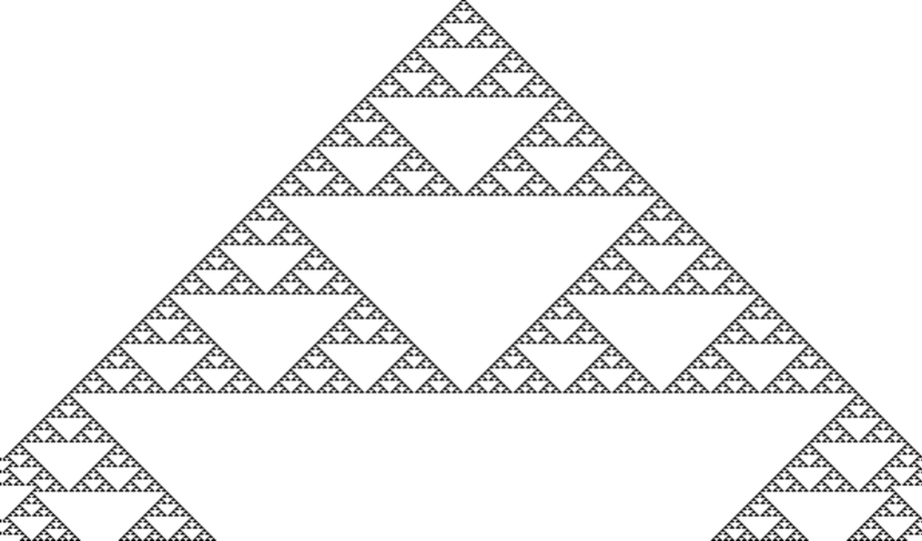
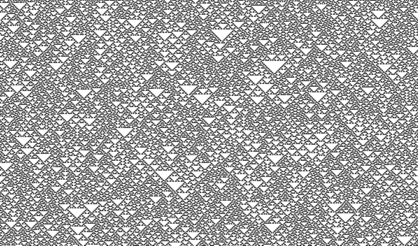
Figure 1: Typical evolution of ECA rule 22 (a) from a single cell in state ‘1’ and (b) from a random initial configuration where half of the cells, chosen at random, are assigned state ‘1’. The ECA consists of 598 cells and evolves for 352 generations. White colour represents state ‘0’ and dark colour represents state ‘1’.

4 Elementary Cellular Automata with Memory

Conventional CA are ahistoric (memoryless): the new state of a cell depends on the neighbourhood configuration solely at the preceding time step of $\varphi$. CA with memory (CAM) can be considered as an extension of the standard framework of CA where every cell $x_{i}$ is allowed to remember some period of its previous evolution. CAM was introduced by Sanz, see overview in [51]. To implement a memory function we need to specify the kind of memory $\phi$, as follows:

$$\phi(x^{t-\tau}_{i},\ldots,x^{t-1}_{i},x^{t}_{i})\rightarrow s_{i}.$$ (2)

The parameter $\tau<t$ determines the depth, or a degree, of the memory and each cell $s_{i}\in\Sigma$ being a state function of the series of states of the cell $x_{i}$ with memory up to time-step. To execute the evolution we apply the original rule as:

$$\varphi(\ldots,s^{t}_{i-1},s^{t}_{i},s^{t}_{i+1},\ldots)\rightarrow x^{t+1}_{i}.$$ (3)

The main feature in CAM is that the mapping $\varphi$ remains unaltered, while historic memory of all past iterations is retained by featuring each cell in the context of history of its past states in $\phi$. This way, cells canalise memory to the map $\varphi$. For example, we can consider memory function $\phi$ as a majority memory $\phi_{maj}\rightarrow s_{i}$, where in case of a tie given by $\Sigma_{1}=\Sigma_{0}$ in $\phi$ we will take the last value $x_{i}$. In this case, function $\phi_{maj}$ represents the classic majority function for three values [37] as follows:

$$(a\wedge b)\vee(b\wedge c)\vee(c\wedge a)$$ (4)

that represents the cells $(x^{t-\tau}_{i},\ldots,x^{t-1}_{i},x^{t}_{i})$ and define a temporal ring of $s$ cells, before reaching the next global configuration $c$.

5 Elementary Cellular Automaton with Memory Rule $\phi_{R22maj:4}$

ECA with memory (ECAM) rule $\phi_{R22maj:4}$ employ the majority memory ($maj$) and degree of memory $\tau=4$.

Figure 2 shows a typical evolution of ECAM rule $\phi_{R22maj:4}$ from a random initial condition. There we observe emergence of gliders travelling and colliding with each other.

localisation	period	shift	velocity	mass
$g_{L}$	11	$-2$	$-2/11$	38
$g_{R}$	11	2	$2/11$	38

Table 1: Properties of gliders in ECAM rule $\phi_{R22maj:4}$.

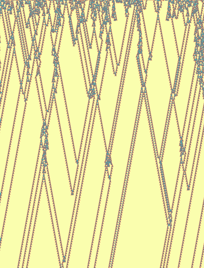
Figure 2: Typical evolution of $\phi_{R22maj:4}$ from a random initial configuration with the ratio of 37% on a ring of 968 cells for 1,274 generations. Filter and a selection of colors are used to improve the view of particles.

The set of gliders ${\cal G}_{\phi_{R22maj:4}}=\{g_{L},g_{R}\}$ are defined in a square of $11\times 11$, their properties are shown in Tab. 1.

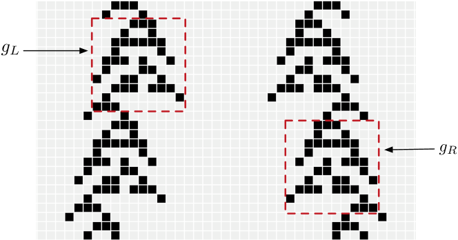
Figure 3: $g_{L}$ and $g_{R}$ gliders in ECAM rule $\phi_{R22maj:4}$.

We undertook a systematic analysis of binary collisions between gliders and found 44 different types of the collision outcomes, we selected some types of the collisions to realise logical gates presented in this paper (see Appendix A).

6 Logic gates via gliders collisions

We assume presence of a glider at a given site of space and time is a logical ‘1’ (True) and absence is ‘0’ (False). Logic gates $f(a,b)\rightarrow\neg a$ $|$ $\neg b$ $|$ $a\wedge b$ are realised via binary collisions of gliders in rule $\phi_{R22maj:4}$. Figure 4bc shows how and-not gate is realised. Fig. 4d demonstrates implementations of and gate. Also a delay operator can be implemented by delaying glider $a$ and conserving momentum of glider $b$ as shown in Fig. 4e

A nand gate can be cascaded from majority and not gates. To design nand gate, we fix third value in majority gate to produce and gate as illustrated in Fig 5b. Later a not gate is cascaded to get a nand gate (Fig. 5a).

Figure 6a represents a value ‘0’ as one glider and a value ‘1’ as a couple of gliders. Figure 6b presents a scheme of nand gate in $\phi_{R22maj:4}$. We have three-input values/gliders that will be evaluated by one control glider travelling perpendicularly to input gliders. The control glider transforms $f(a,b,c)$ into a majority function. Further, other glider acts as an active signal in not gate.

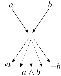
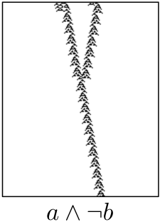
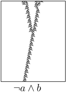
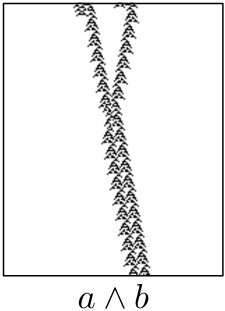
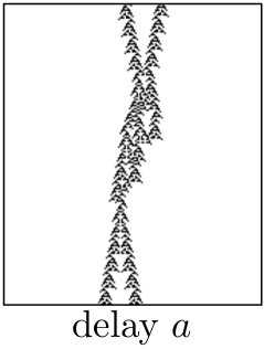
Figure 4: Examples of logical gates implemented via glider collisions. Presence of a glider is logical Truth ‘1’, absence logical False ‘0’. (a) Scheme of the gate. (bc) and-not gate, (d) and, (e) delay

.

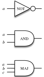
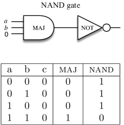
Figure 5: Gate nand made of majority and not gates. (a) Schematics of gates. (b) Design of nand gate.

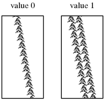
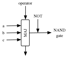
Figure 6: Gate majority. (a) Binary values represented by gliders, (b) scheme of an nand gate using majority and not gates.

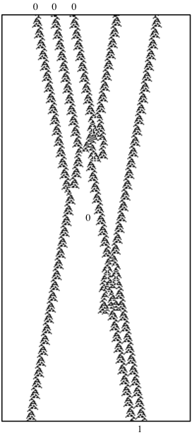
Figure 7: Gate nand implemented with majority and not gates in ECAM rule $\phi_{R22maj:4}$ following the scheme proposed in Fig. 6b. (a) Input values $f(0,0,0)$ and (b) input values $f(0,1,0)$. Intervals between gliders in the initial condition are the same in all operations.

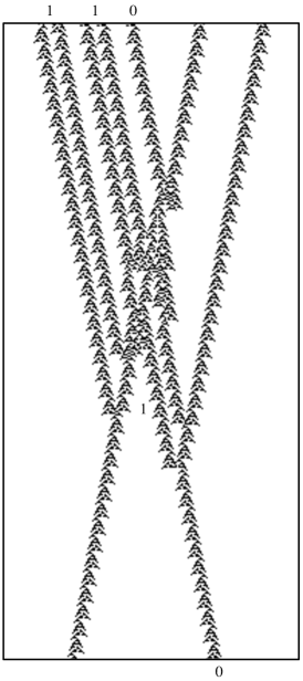
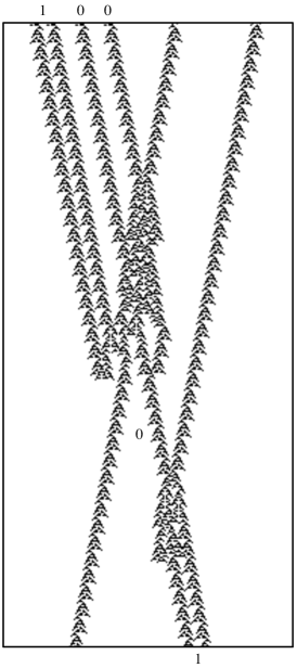
Figure 8: Gate nand implemented with majority and not gates in ECAM rule $\phi_{R22maj:4}$ following the scheme proposed in Fig. 6b. (a) Input values $f(1,1,0)$ and (b) input values $f(1,0,0)$.

Figures 7 and  8 show the implementation of nand gate in $\phi_{R22maj:4}$, encoded in its initial condition set of gliders in six positions. As was shown in the scheme (Fig. 6c), gliders coming from the left side represent binary values and a glider coming from the right acts as a control glider for the values of the majority gate. The control glider continues its travel undisturbed, after interaction with input gliders, and therefore it can be recycled in further majority gate.

6.1 Ballistic collisions

A concept of ballistic logical gates represent Boolean values by balls which preserve their identity during collision but change their velocity vectors; the balls are routed in the computing space using mirrors [58]. The billiard ball model was advanced by Margolus in his designs of partitioned CA to demonstrate a logical universality of a billiard-ball model and to implement Fredkin gate with soft spheres in billiard-ball model [28, 29].

Ballistic collisions of gliders, or particles, permit to represent functions of two arguments (general signal-interaction scheme is conceptualized in Fig. 9a), as follows [58]:

1. $f(u,v)$ is a product of one collision (Fig. 9b);

2. $f_{i}(u,v)\mapsto(u,v)$ identity (Fig. 9c);

3. $f_{r}(u,v)\mapsto(v,u)$ reflection (Fig. 9d);

where Fig. 9a represents a collision not preserving identity of gliders $u$ and $v$; Fig. 9b shows a collision where identities of input gliders are preserved.

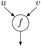
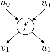
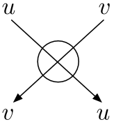
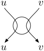
Figure 9: Schematics of ballistic collisions implemented with gliders.

Below we show that ECAM rule $\phi_{R22maj:4}$ reproduces ballistic collisions. Figure 10 demonstrates identity collisions $f_{i}(u,v)\mapsto(u,v)$. The collisions between gliders are illustrated in (Fig. 10). The collisions are of soliton nature [20, 56]. A carry-ripple adder [55] can be implemented in ECAM Rule $\phi_{R22maj:4}$ by solitonic reactions with pairs of gliders and identity function (Fig. 10a).

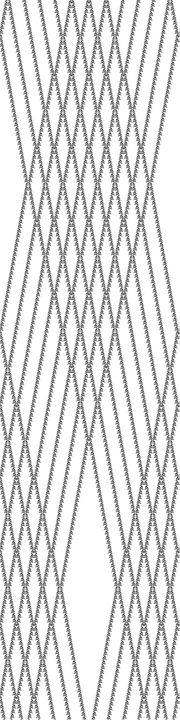
Figure 10: Implementation of ballistic collisions in ECAM rule $\phi_{R22maj:4}$. (a) 20 gliders are synchronised to simulate the function identity $f_{i}(u,v)\mapsto(u,v)$, (b) 18 gliders preserve their identity during collisions. ECAM is a ring of 418 cells. It evolved in 1697 time steps.

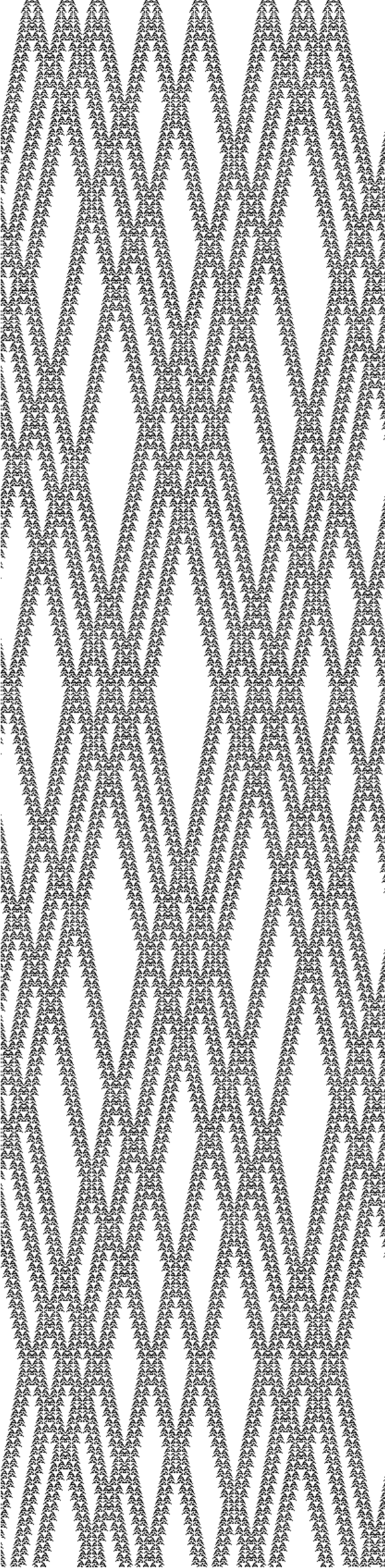
Figure 11: Implementation of ballistic collisions in ECAM rule $\phi_{R22maj:4}$. (a) Pairs of six gliders are synchronised to simulate the reflections or elastic collisions $f_{r}(u,v)\mapsto(v,u)$, (b) 16 pairs of gliders preserve their identity during collisions. ECAM is a ring of 418 cells. It evolved in 1697 time steps.

Figure 11 illustrates elastic collisions $f_{r}(u,v)\mapsto(v,u)$ with a pair of gliders. The pairs of gliders reflect in the same manner in all collisions (Fig. 11a). These elastic collisions are robust to phase changes and initial positions of gliders (Fig. 11b).

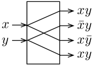
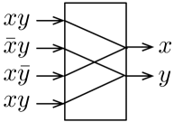
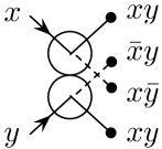
Figure 12: In ballistic collisions we can implement an (a) interaction gate, (b) its inverse, and (c) its billiard ball model realisation.

The ballistic interaction gate (Fig. 12a) is invertible (Fig. 12b) [10]. Therefore inverse and elastic collisions in $\phi_{R22maj:4}$ may model the interaction gate: gliders $g_{R}$ and $g_{L}$ are equivalent to balls. To allow gliders to return to the original input locations we may constrain them with boundary conditions (Figs. 10 and 11) or route them with mirrors.

6.2 Fredkin gate

A conservative logic gate is a Boolean function that is invertible and preserve signals [17]. Fredkin gate is a classical conservative logic gate. The gate realises the transformation $(c,p,q)\mapsto(c,cp+\bar{c}q,cq+\bar{c}p)$, where $(c,p,q)\in\{0,1\}^{3}$. Schematic functioning of Fredkin gate is shown in Fig. 13 and the truth table is in Table 2.

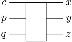
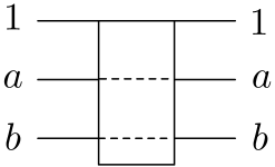
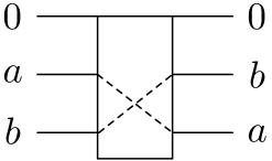
Figure 13: Fredkin gate. (a) Scheme of the gate, (b) operation for control value 1, (c) operation for control value 0.

$c$	$p$	$q$		$x$	$y$	$z$
0	0	0		0	0	0
0	0	1		0	1	0
0	1	0		0	0	1
0	1	1	$\rightarrow$	0	1	1
1	0	0		1	0	0
1	0	1		1	0	1
1	1	0		1	1	0
1	1	1		1	1	1

Table 2: Truth table of Fredkin gate.

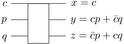
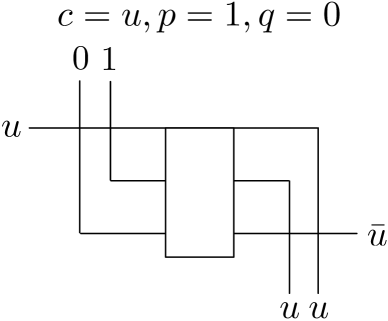
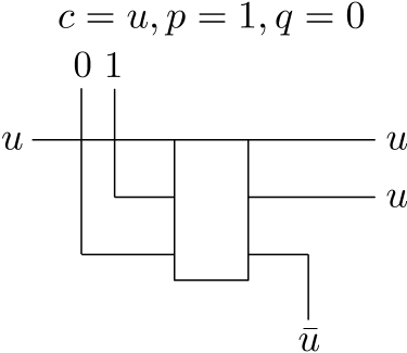
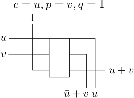
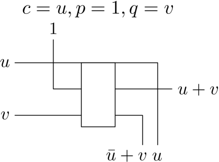
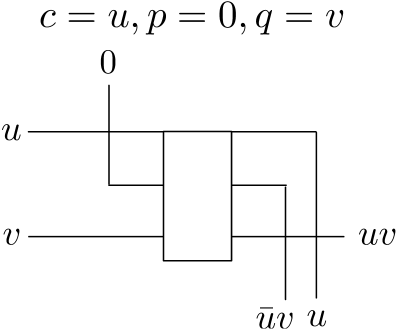
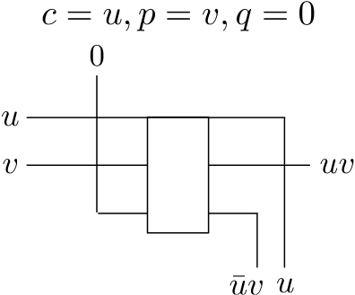
Figure 14: Realisation of Boolean functions using Fredkin gate. (a) Fredkin gate, (b) not gate, (c) fanout gate, (d-e) or gate, and (f-g) and gate [17].

Fredkin gate is universal because one can implement a functionally complete set of logical functions with this gate (Fig. 14). Other gates implemented with Fredkin gate are shown below:

• $c=u$, $p=v$, $q=1$ (or $c=u$, $p=1$, $q=v$) yields the implies gate $y=u\rightarrow v$ $(z=u\rightarrow v)$.

• $c=u$, $p=0$, $q=v$ (or $c=u$, $p=v$, $q=0$) yields the not implies gate $y=\overline{(v\rightarrow u)}$ $(z=\overline{(v\rightarrow u)})$ [17].

6.3 Basic collisions

To simulate a Fredkin gate in ECAM rule $\phi_{R22maj:4}$, we utilise a set of collisions to preserve the reactions and the persistence of data, these basic collisions have a specific task and actions which are specified as follows.

• Mirror reflects a glider, the mirror should be deleted, not to become an obstacle for other signals.

• Doubler splits a signal into two signals.

• Soliton crosses two gliders preserving its identity but might change its phase.

• Splitter separates two gliders into gliders travelling in opposite directions.

• Flag is a glider that is generated depending of an input value given.

• Displacer moves a glider forward.

Fredkin gates implemented in non-invertible systems were proposed and simulated by Adamatzky in a non-linear medium — Oregonator model of Belousov-Zhabotinsky [7].

Figure 15: A scheme of Fredkin gate implementation in ECAM rule $\phi_{R22maj:4}$ via glider collisions.

6.4 Fredkin gates in one dimension

Figure 15 displays the schematic diagram proposed to simulate Fredkin gates in ECAM rule $\phi_{R22maj:4}$. There are three inputs $(c,p,q)$ and three outputs $(x,y,z)$. During the computation auxiliary gliders are generated. They are deleted before reaching outputs. Gliders travel in two directions in a 1D chain of cells, they can be reused only when crossing periodic boundaries or via combined collisions. We use two gliders as flags, travelling from the left ‘$L_{f}$’ and from the right ‘$R_{f}$’. Flags are activated depending on initial values for $c$ or $q$ as follows

• If $c=0$ then $R_{f}=1$,

• If $q=0$ then $L_{f}=1$,

• In any other case $L$ and $R=0$.

Mirrors $M$ are defined as follows:

• If $c=p=q=1$ then $M=2$,

• If $c=p=1$ then $M=2$,

• If $c=q=1$ then $M=1$,

• If $p=1$ then $M=1$,

• In any other case $M=0$.

Distances between gliders are fixed as positive integers determined for a number of cells in the state ‘0’, as $\stackrel{{\scriptstyle\text{\tiny$0^{n}$}}}{{\frown}}$ $\forall$ $n\geq 0$. During the computation we split gliders when two gliders travel together, the split gliders travel in opposite directions. We use two gliders as mirrors to change the direction of an argument movement. We use displacer to move an output glider and adjust its distance with respect to other.

$cpq$	$xyz$	$L_{f}$	$R_{f}$	M
111	111	0	0	2
110	110	1	0	2
101	101	0	0	1
100	100	1	0	0
011	011	0	1	0
010	001	1	1	1
001	010	0	1	0

Table 3: Following the scheme in Fig. 15 we specify a sequence of collisions that are controlled with flag gliders ($L_{f}$, $R_{f}$) and mirrors (M) glider.

Table 3 shows values of inputs, outputs, flags, and mirrors. First column represents inputs, the second column outputs, third column are values of a flag activated in the left side, fourth column are values of the flag activated in the right side, and the last column shows the number of necessary mirrors.

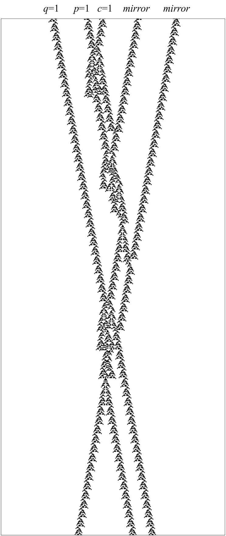
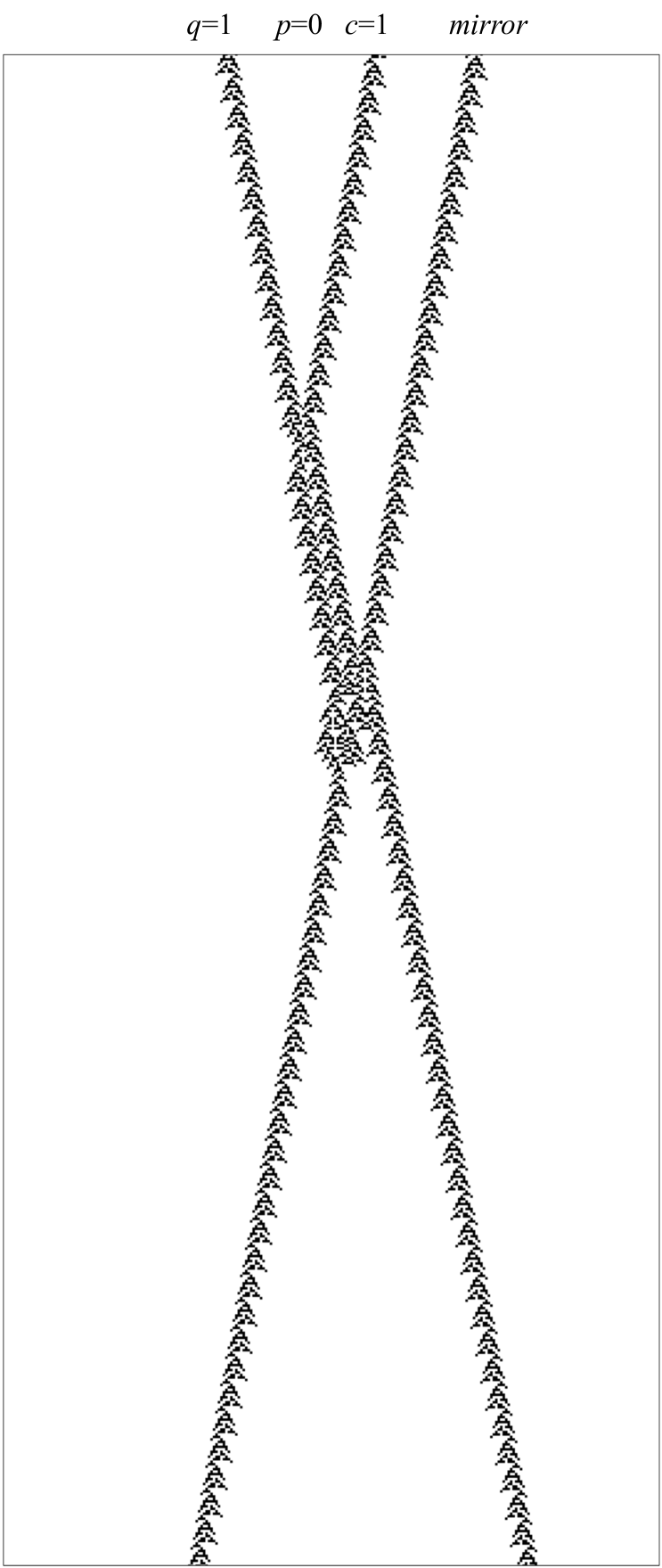
Figure 16: Fredkin gate in ECAM rule $\phi_{R22maj:4}$. (a) INPUT $c=1$, $p=1$, $q=1$, OUTPUT $x=1$, $y=1$, $z=1$, (b) INPUT $c=1$, $p=0$, $q=1$, OUTPUT $x=1$, $y=0$, $z=1$.

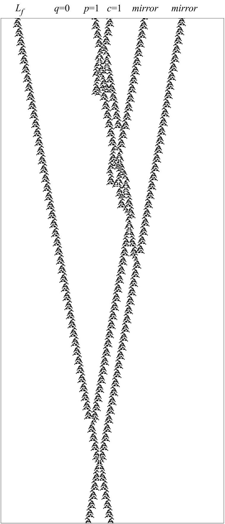
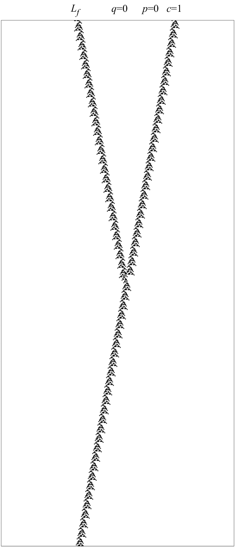
Figure 17: Fredkin gate in ECAM rule $\phi_{R22maj:4}$. (a) INPUT $c=1$, $p=1$, $q=0$, OUTPUT $x=1$, $y=1$, $z=0$, (b) INPUT $c=1$, $p=0$, $q=0$, OUTPUT $x=1$, $y=0$, $z=0$.

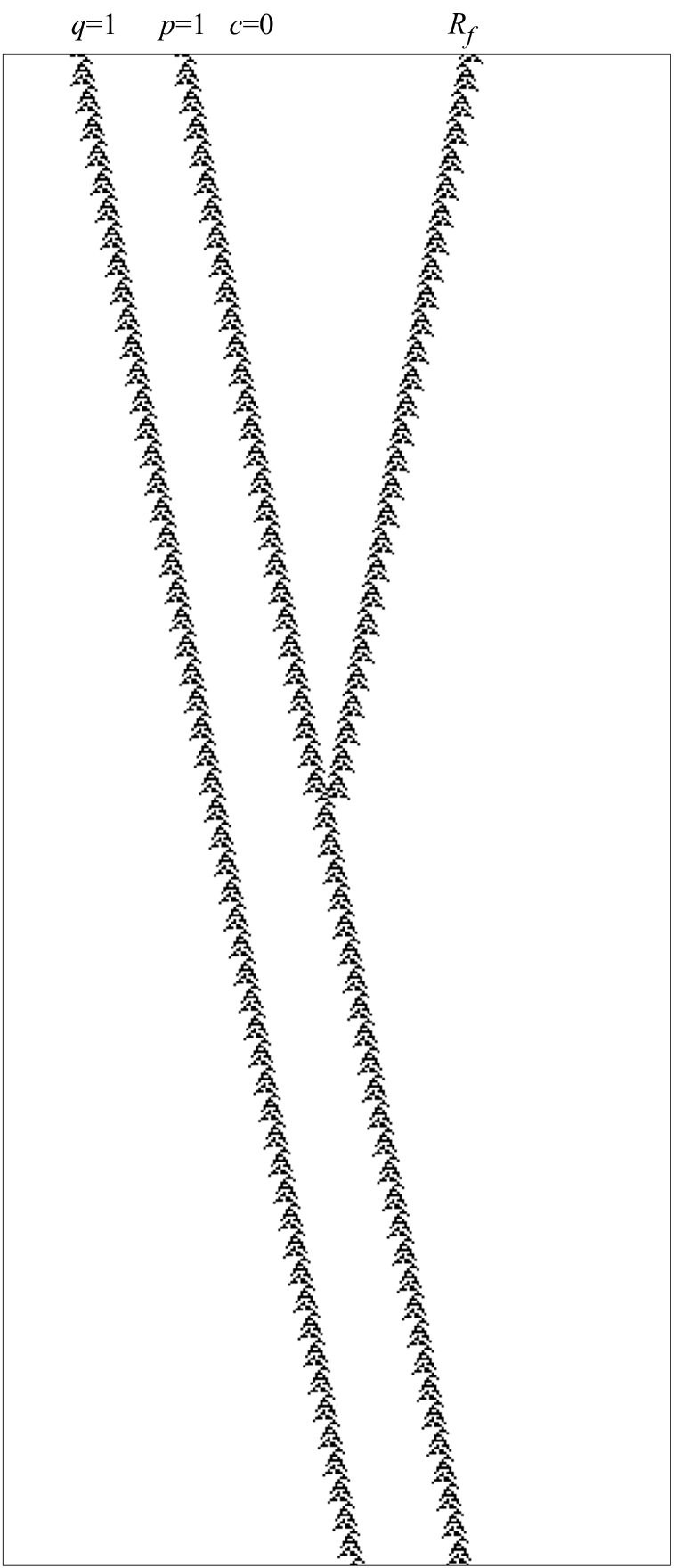
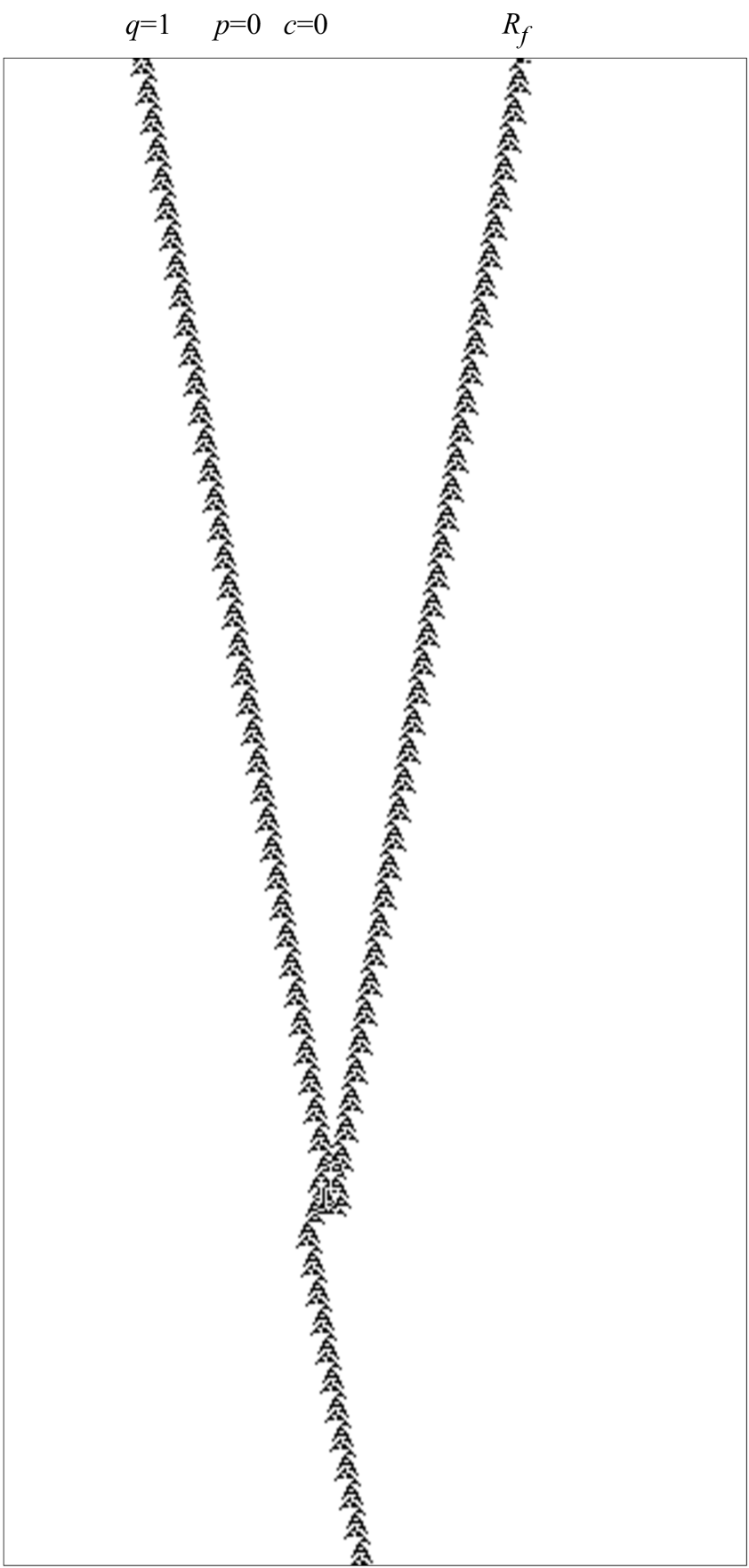
Figure 18: Fredkin gate in ECAM rule $\phi_{R22maj:4}$. (a) INPUT $c=0$, $p=1$, $q=1$, OUTPUT $x=0$, $y=1$, $z=1$, (b) INPUT $c=0$, $p=0$, $q=1$, OUTPUT $x=0$, $y=1$, $z=0$.

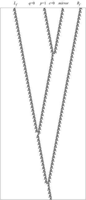
Figure 19: Fredkin gate in ECAM rule $\phi_{R22maj:4}$. INPUT $c=0$, $p=1$, $q=0$, OUTPUT $x=0$, $y=0$, $z=1$.

Space-time configurations of ECAM rule $\phi_{R22maj:4}$ implementing Fredkin gate for all non-zero combinations of inputs are shown in Figs. 16–19.

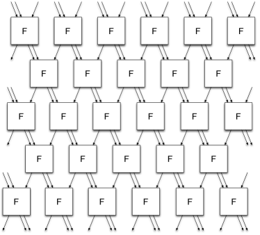
Figure 20: Cascaded Fredkin gates (It is a modification of Fredkin array proposed  [30]).

7 Discussion

We demonstrated how to implement a functionally complete set of Boolean functions in a one-dimensional cellular automaton with binary cell states, three-cell neighbourhood and memory depth four. We also shown that Fredkin gate can be realised the this automaton. Let us compare complexity of our designs with previously published models of universal one-dimensional cellular automata.

CA simulating Turing machine, proposed by Smith III in 1971 [52], satisfied the condition: a number of cell-states multiplied by a neighbourhood size equals $\eta=36$. A universal 1D CA designed by Albert and Culik II [1] has 14 states and totalistic cell-state transition rule, that is for their automaton $\eta=42$. The Lindgren-Nordahl CA [21] has 7 states, assuming three-cell neighbourhood we have $\eta=21$. ECAM implementation of a Fredkin gate, proposed in present paper, has two cell states, three cell neighbourhood, and memory depth 4, this implies $\eta=24$. Thus, in terms of a neighbourhood size and a number of states our automaton is less efficient than the CA proposed by Lindgren-Nordahl [21], however we use gliders as signals. Gliders are discrete analogs of solitons, therefore our design, in principle, can be considered as a blueprint for physical implementation, as we will discuss below. Cook’s design [13, 64] of a universal CA via cyclic tag system is the most optimal in terms of neighbourhood size and number of states, $\eta=6$, however the implementation involves 11 gliders and a glider gun. Our design of Fredkin gate utilises just two types of gliders.

Polymer chains that support propagation of travelling localisations (solitons, kinks, defects) are potential substrates for implementation of glider-based Fredkin gate. There are many potential candidates, here we discuss actin filaments. Actin is a protein presented in all eukaryotic cells in forms of globular actin (G-actin) and filamentous actin (F-actin), see history overview in [53]. Filamentous actin is a double helix of F-actin unit chains. In [6] we proposed a model of actin polymer filaments as two chains of one-dimensional binary-state semi-totalistic automaton arrays and uncovered rules supporting gliders, discrete analogs of ionic waves propagating in actin filaments [59].

Let us evaluate a physical space-time requirement for implementation of Fredkin gate on actin filaments. Assume a unit of F-actin corresponds to a cell of 1D CA. Maximum diameter of an actin filament is 8 nm [40, 54]. An actin filament is composed of overlapping units of F-actin. Thus, diameter of a single unit is c. 4 nm. A glider in our ECAM model occupies 10 cells, that makes a size of a signal in actin filaments 40 nm. Maximum distance between inputs in ECAM Fredkin gate is 200 cells. This makes gate size 880 nm.

With regards to speed of Fredkin gate realisation, being unaware of exact mechanisms of travelling localisations on actin filaments we can propose speculative estimates. Assume the underpinning mechanism of generating a localisation is an excitation of F-actin molecule (single unit of actin polymer). An excitation in a molecule takes place when an electron in a ground state absorbs a photon and moves up to a high yet unstable energy level. Later the electron returns to its ground state. When returning to the ground state the electron releases photon which travels with speed $\times 10^{18}$ Å  per second. F-actin molecule (one unit of actin filament) is a polymer chain of at most 3K nodes. Thus the F-actin unit can be spanned by an excitation in at most $10^{-15}$ sec. That can be adopted as a physical time step equivalent to one step of ECAM evolution. The ECAM Fredkin gate completes its operation on actin filament in 600 time steps, that is at most $10^{-13}$ sec, i.e. 0.1 picosecond of real time.

Experimental implementation of the Fredkin gate, including cascading of the gates, on actin filaments, or any other soliton-supporting polymer chain makes a very challenging topic of future studies. There methodological approaches to control and monitor attosecond scale molecular dynamics  [14, 8, 48, 11] however it is not clear if they can be applied to actin polymers. The problems to overcome include input of data in acting filament with a single F-actin unit precision, keeping the polymer chain stable and insulated from thermal noise, reading outputs from the polymer chain. However exact experimental implementation remains uncertain.

But, although this can be confined in a physical computing device several limitations should be improved: avoid the use of mirrors and the use of flags. An option is that they could be manipulated into in a ring (or virtual CA collider [32, 27]).

Appendix A Appendix – Binary collisions in $\phi_{R22maj:4}$

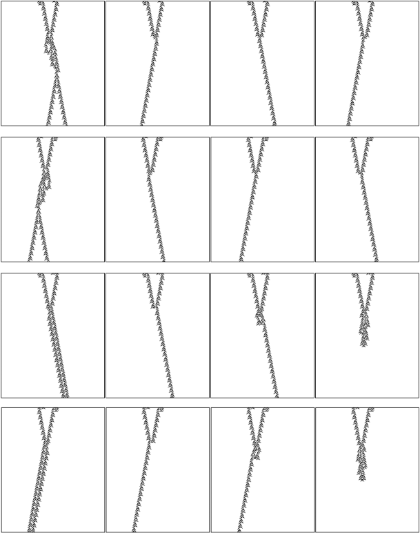
Figure 21: Binary collisions in Rule 22 with memory.

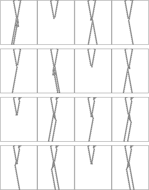
Figure 22: Binary collisions in Rule 22 with memory.

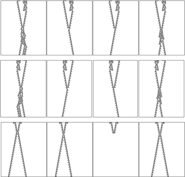
Figure 23: Binary collisions in Rule 22 with memory.

References

- [1] Albert, J. & Culik II, K. (1987) A simple universal cellular automaton and its one-way and totalistic versions, Complex Systems 1(1) 1–16.
- [2] Adamatzky, A. (2001) Computing in Nonlinear Media and Automata Collectives, IOP Publishing Ltd. Bristol, UK.
- [3] Adamatzky, A. (Ed.) (2002) Collision-Based Computing, Springer.
- [4] Adamatzky, A., Costello, B.L. & Asai, T. (2005) Reaction-Diffusion Computers, Elsevier.
- [5] Adamatzky, A. (2010) Physarum Machines: Computers from Slime Mould, World Scientific Series on Nonlinear Science Series A: Volume 74.
- [6] Adamatzky, A. & Mayne, R. (2015) Actin automata: Phenomenology and localizations, International Journal of Bifurcation and Chaos 25(02) 1550030.
- [7] Adamatzky, A. (2017) Fredkin and Toffoli gates implemented in oregonator model of Belousov-Zhabotinsky medium, Int. J. Bifurcation and Chaos 27(3) 1750041.
- [8] Baltuska, A., Udem, T., Uiberacker, M., Hentschel, M., Goulielmakis, E., Gohle, C., Holzwarth, R., Yakovlev, V.S., Scrinzi, A., Hansch, T.W. & Krausz, F. (2003) Attosecond control of electronic processes by intense light fields, Nature 421(6923) 611–615.
- [9] Banks, E.R. (1971) Information and transmission in cellular automata, PhD Dissertion, Cambridge, MA, MIT.
- [10] Bennett, C.H. (1973) Logical reversibility of computation, IBM Journal of Research and Development 17(6) 525–532.
- [11] Ciappina, M.F., Hernández, J.P., Landsman, A., Okell, W., Zherebtsov, S., Förg, B., Schötz, J., Seiffert, L., Fennel, T., Shaaran, T. & Zimmermann, T. (2017) Attosecond physics at the nanoscale, Reports on Progress in Physics 80(5) 054401.
- [12] Codd, E.F. (1968) Cellular Automata, Academic Press, Inc. New York and London.
- [13] Cook, M. (2004) Universality in Elementary Cellular Automata, Complex Systems 15(1) 1–40.
- [14] Goulielmakis, E., Schultze, M., Hofstetter, M., Yakovlev, V.S., Gagnon, J., Uiberacker, M., Aquila, A.L., Gullikson, E.M., Attwood, D.T., Kienberger, R. and Krausz, F. (2008) Single-cycle nonlinear optics, Science 320(5883) 1614–1617.
- [15] Moore, C. & Mertens, S. (2011) The Nature of Computation, Oxford University Press.
- [16] Fredkin, E. & Toffoli, T. (2002) Design Principles for Achieving High-Performance Submicron Digital Technologies. In: Collision-Based Computing, A. Adamatzky (ed), Springer, chapter 2, pages 27–46.
- [17] Fredkin, E. & Toffoli, T. (1982) Conservative logic, Int. J. Theoret. Phys. 21 219–253.
- [18] Hey, A.J.G. (1998) Feynman and computation: exploring the limits of computers, Perseus Books.
- [19] Hutton, T.J. (2010) Codd’s self-replicating computer, Artificial Life 16(2) 99–117.
- [20] Jakubowski, M.H., Steiglitz, K. & Squier, R. (2001) Computing with Solitons: A Review and Prospectus, Multiple-Valued Logic 6(5-6) 439–462. (also republished in [3])
- [21] Lindgren, K. & Nordahl M. (1990) Universal Computation in Simple One-Dimensional Cellular Automata, Complex Systems 4 229–318.
- [22] Martínez, G.J., Adamatzky, A., Sanz, R.A. & Mora, J.C.S.T. (2010) Complex dynamic emerging in Rule 30 with majority memory, Complex Systems 18(3) 345–365.
- [23] Martínez, G.J., Adamatzky, A. & Sanz, R.A. (2012) Complex dynamics of elementary cellular automata emerging in chaotic rule, Int. J. of Bifurcation and Chaos 22(2) 1250023-13.
- [24] Martínez, G.J., Adamatzky, A. & Sanz, R.A. (2013) Designing Complex Dynamics with Memory, Int. J. Bifurcation and Chaos 23(10) 1330035-131.
- [25] Martínez, G.J., Adamatzky, A., Chen, F. & Chua, L. (2012) On Soliton Collisions between Localizations in Complex Elementary Cellular Automata: Rules 54 and 110 and Beyond, Complex Systems 21(2) 117–142.
- [26] Martínez, G.J., Adamatzky, A. & McIntosh, H.V. (2006) Phenomenology of glider collisions in cellular automaton Rule 54 and associated logical gates, Chaos, Solitons and Fractals 28 100–111.
- [27] Martínez, G.J., Adamatzky, A., & McIntosh, H.V. (2016) A Computation in a Cellular Automaton Collider Rule 110, In: Advances in Unconventional Computing Volume 1: Theory, A. Adamatzky (Ed.), Springer, chapter 15, 391–428.
- [28] Margolus, N.H. (1984) Physics-like models of computation, Physica D 10 (1-2) 81–95.
- [29] Margolus, N.H. (1998) Crystalline Computation, In: Feynman and computation: exploring the limits of computers, A.J.G. Hey (Ed.), Perseus Books, 267–305.
- [30] Margolus, N.H. (2002) Universal Cellular Automata Based on the Collisions of Soft Spheres, In: Collision-Based Computing, A. Adamatzky (Ed.), Springer, chapter 5, 107–134.
- [31] Martínez, G.J., Adamatzky, A., Mora, J.C.S.T. & Alonso-Sanz, R. (2010) How to make dull cellular automata complex by adding memory: Rule 126 case study, Complexity 15(6) 34–49.
- [32] Martínez, G.J., Adamatzky, A., Stephens, C.R. & Hoeflich, A.F. (2011) Cellular automaton supercolliders, International Journal of Modern Physics C 22(4) 419–439.
- [33] McIntosh, H.V. (1990) Wolfram’s Class IV and a Good Life, Physica D 45 105–121.
- [34] McIntosh, H.V. (2009) One Dimensional Cellular Automata, Luniver Press.
- [35] Morita, K. & Harao, M. (1989) Computation universality of one-dimensional reversible (injective) cellular automata, Trans. IEICE Japan E-72 758–762.
- [36] Mills, J.W. (2008) The Nature of the Extended Analog Computer, Physica D 237(9) 1235–1256.
- [37] Minsky, M. (1967) Computation: Finite and Infinite Machines, Prentice Hall.
- [38] Mitchell, M. (2001) Life and evolution in computers, History and Philosophy of the Life Sciences 23 361–383.
- [39] Martínez, G.J., McIntosh, H.V., Mora, J.C.S.T. & Vergara, S.V.C. (2011) Reproducing the cyclic tag system developed by Matthew Cook with Rule 110 using the phases f1_1, Journal of Cellular Automata 6(2-3) 121–161.
- [40] Moore, P.B., Huxley, H.E. & DeRosier, D.J. (1970) Three-dimensional reconstruction of F-actin, thin filaments and decorated thin filaments, Journal of Molecular Biology 50(2) 279–288.
- [41] Morita, K. (1990) A simple construction method of a reversible finite automaton out of Fredkin gates, and its related problem, Trans. IEICE Japan E-73 978–984.
- [42] Morita, K. (2000) A new universal logic element for reversible computing, IEICE technical report. Theoretical foundations of Computing 99(724) 119–126.
- [43] Morita, K. (2007) Simple universal one-dimensional reversible cellular automata, Journal of Cellular Automata 2 159–165.
- [44] Morita, K. (2008) Reversible computing and cellular automata—A survey, Theoretical Computer Science 395 101–131
- [45] Morita, K. (2016) Universality of 8-State Reversible and Conservative Triangular Partitioned Cellular Automata, Lecture Notes in Computer Science 9863 45–54
- [46] Martínez, G.J., Mora, J.C.S.T. & Zenil, H. (2013) Computation and Universality: Class IV versus Class III Cellular Automata, Journal of Cellular Automata 7(5-6) 393–430.
- [47] Margolus, N., Toffoli, T. & Vichniac, G. (1986) Cellular-Automata Supercomputers for Fluid Dynamics Modeling, Physical Review Letters 56(16) 1694–1696.
- [48] Nabekawa, Y., Okino, T. & Midorikawa, K. (2017) Probing attosecond dynamics of molecules by an intense a-few-pulse attosecond pulse train. In: 31st International Congress on High-Speed Imaging and Photonics, pp. 103280B. International Society for Optics and Photonics, Osaka, Japan.
- [49] Park, J.K., Steiglitz, K. & Thurston, W.P. (1986) Soliton-like behavior in automata, Physica D 19 423–432.
- [50] Rendell, P. (2016) Turing Machine Universality of the Game of Life, Springer.
- [51] Sanz, R.A. (2009) Cellular Automata with Memory, Old City Publishing.
- [52] Smith III, A.R. (1971) Simple computation-universal cellular spaces, J. of the Assoc. for Computing Machinery 18 339–353.
- [53] Szent-Gyórgyi, A.G. (2004). The early history of the biochemistry of muscle contraction, Journal of General Physiology 123(6) 631–641.
- [54] Spudich, J.A., Huxley, H.E. & Finch, J.T. (1972) Regulation of skeletal muscle contraction: II. Structural studies of the interaction of the tropomyosin-troponin complex with actin, Journal of molecular biology 72(3) 619–632.
- [55] Steiglitz, K., Kamal, I. & Watson, A. (1988) Embedding Computation in One-Dimensional Automata by Phase Coding Solitons, IEEE Transactions on Computers 37(2) 138–145.
- [56] Steiglitz, K. (2016) Soliton-Guided Quantum Information Processing, In: Advances in Unconventional Computing Volume 2: Prototypes, Models and Algorithms, A. Adamatzky (Ed.), Springer, chapter 13, 297–307.
- [57] Toffoli, T. (1998) Non-Conventional Computers, In: Encyclopedia of Electrical and Electronics Engineering, J. Webster (Ed.), 14 455–471, Wiley & Sons.
- [58] Toffoli, T. (2002) Symbol Super Colliders, In: Collision-Based Computing, A. Adamatzky (Ed.), Springer, chapter 1, 1–22.
- [59] Tuszyński, J.A., Portet, S., Dixon, J.M., Luxford, C. & Cantiello, H.F. (2004) Ionic wave propagation along actin filaments, Biophysical Journal 86(4) 1890–1903.
- [60] von Neumann, J. (1966) Theory of Self-reproducing Automata (edited and completed by A. W. Burks), University of Illinois Press, Urbana and London.
- [61] Wolfram, S. (1984) Universality and complexity in cellular automata, Physica D 10 1–35.
- [62] Wolfram, S. (1984) Computation Theory of Cellular Automata, Communications in Mathematical Physics 96 15–57.
- [63] Wolfram, S. (1994) Cellular Automata and Complexity, Addison-Wesley Publishing Company.
- [64] Wolfram, S. (2002) A New Kind of Science, Wolfram Media, Inc., Champaign, Illinois.