Braess paradox in a network with stochastic dynamics and fixed strategies

Abstract

The Braess paradox can be observed in road networks used by selfish users. It describes the counterintuitive situation in which adding a new, per se faster, origin-destination connection to a road network results in increased travel times for all network users. We study the network as originally proposed by Braess but introduce microscopic particle dynamics based on the totally asymmetric exclusion processes. In contrast to our previous work [1], where routes were chosen randomly according to turning rates, here we study the case of drivers with fixed route choices. We find that travel time reduction due to the new road only happens at really low densities and Braess’ paradox dominates the largest part of the phase diagram. Furthermore, the domain wall phase observed in [1] vanishes. In the present model gridlock states are observed in a large part of phase space. We conclude that the construcion of a new road can often be very critical and should be considered carefully.

1 Introduction

Urbanization is one of the big challenges of modern times. As the world population grows, more and more people are moving into cities [2]. With the growing population sizes, also the transportation network has to adapt. The expansion of the city and its transportation network, an interplay of top-down planning and self-organizational processes [3], has to be considered carefully to be efficient. The Braess paradox was discovered by D. Braess in 1968 [4, 5]. He proposed a specific road network in which adding a new road counterintuitively leads to higher travel times for all the network users given that they minimize their own travel times selfishly. The network consists of four individual roads forming two possible routes from start to finish. Then a new road is added resulting in a new per se faster route from start to finish. A state of the system is characterized by the distribution of the vehicles onto the available roads. If a certain amount of drivers wants to go from start to finish and they all want to minimize their own travel times, the system is in a stable state if all used routes have the same travel time which is shorter than the travel times of any unused routes. This is the so-called user optimum [6] or Nash equilibrium of the system. Braess showed that for specific combinations of travel time functions of the roads and the total number of cars, the user optimum of the system with the new road has higher travel times than that of the system without the new road. This appears to be a paradox since one would assume that an additional route increases the capacity and thus leads to a decrease of travel times.

Many efforts have been made in understanding Braess’ paradox in more general terms. Indeed it was shown that its occurrence is very prevalent in congested networks [7]. The regions of its occurrence in certain models were determined [8, 9] and it was also shown to occur in certain real-world scenarios [10]. Furthermore, analogues of the paradox were e.g. found in mechanical networks [11], energy networks [12], pedestrian dynamics [13] or thermodynamic systems [14]. In most studies on the paradox the focus was on macroscopical mathematical models of car traffic in which the roads are treated as uncorrelated. Travel times of the roads are given by functions which are linear in the number of cars using the roads. This lead to the discovery, a general understanding and also the observation of the effect in the real world and sparked the ongoing fascination with this counterintuitive phenomenon. Nevertheless, linear travel time functions and the fact that in those models there are no correlation effects between the roads results in a rather unrealistic description of traffic in the network.

It is important to gain a deeper understanding of the paradox in more realistic scenarios since this is relevant for the design of new roads in real road networks. Especially the effects of a more realistic microscopic dynamics and also inter-road correlations like jamming effects or conflicts at road junctions need to be understood. In a recent article [1] we have studied Braess’ network where the dynamics on the edges is given totally asymmetric exclusion processes (TASEPs). The TASEP is a simple cellular automaton [15] and is now renowned as the paradigmatic model for single-lane traffic. It covers a lot of effects which are not included in deterministic mathematical models. In [1] we studied the case where all drivers are identical and choose their routes stochastically. The route choice is determined through the turning probability on the junction sites. We found that the paradox occurs at intermediate global densities $0.1\lesssim\rho_{\text{global}}\lesssim 0.3$. A large part of the phase diagram is dominated by the so-called fluctuation-dominated regime in which no stable travel times can be measured due to domain walls of fluctuating positions (i.e. traffic jams of fluctuating lengths).

In the present paper we analyse the same network with TASEP dynamics on the edges. Instead of a random route choice based on turning probabilities at junctions the particles have fixed routes. This corresponds e.g. to the scenario of daily commuters who stick to their ’favourite’ routes. In the present model stable travel times can be found throughout the whole phase diagram. The fluctuation-dominated regime which is a defining phase for the model we studied previously disappears. Braess’ paradox is found to be even more prevalent in the present case as the system shows Braess-like behaviour in almost the whole phase space for densities $\rho_{\text{global}}\gtrsim 0.1$. This implies that the paradox is even more prominent and important in networks of microscopic transport models than we concluded due to our findings in [1].

2 Model definition

2.1 The totally asymmetric exclusion process

The TASEP is a one-dimensional paradigmatic stochastic transport model. A single TASEP consists of $L$ cells ($L$ is also called the length of a TASEP) which can be either empty or occupied by one particle. In our analysis we use the so-called random sequential update rules. With this update scheme, the dymanics works as follows: With uniform probability one of the $L$ cells is chosen. If this cell is occupied by a particle, the particle can jump to the next cell iff the next cell is empty (see Figure 1). After $L$ of those updates, one timestep is completed. In the case of open boundary conditions, particles are fed onto site 1 from a reservoir which is occupied with the entrance-probability $\alpha$. Particles can leave the system from site $L$ with the exit probability $\beta$. In the case of periodic boundary conditions site $L+1$ is identified with site 1. Thus the total number of particles $M$ in the system is constant and the system effectively becomes a ring.

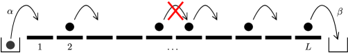
Figure 1: A single TASEP of length $L$ with open boundary conditions. In the case of random sequential update rules a site is chosen randomly. If it is occupied, the particle can jump to the next site if this next site is empty.

In the stationary state of the periodic boundary case the density profile is flat and the local density on each site $i$ equals the global density $\rho(i)=\rho_{\text{global}}=M/L$. In this case, the travel time, i.e. the number of timesteps a particle needs to complete one round, is given by

$$T=\frac{L}{1-\rho}.$$ (1)

The stationary state can also be determined analytically for open boundary conditions [16, 17, 18]. In this case, Equation (1) is a good approximation for the travel times for most combinations of $\alpha$ and $\beta$ if the density is replaced by the average bulk density of the open system [1].

2.2 Braess’ network

We consider the network shown in Figure 2 which is the network introduced by Braess in his original paper [4, 5] but apply periodic boundary conditions. We examine the case that all particles want to go from the start at junction site $j_{1}$ to the finish at junction site $j_{4}$. The edges $E_{i}$ ($i=0,\dots,5$) of the network are TASEPs of lengths $L_{i}$ joined through junction sites $j_{k}$ ($k\in 1,\dots,4$). The junction sites behave as ordinary TASEP cells. They can take one particle at a time. Periodic boundary conditions are achieved through $E_{0}$ with $L_{0}=1$, coupling $j_{4}$ to $j_{1}$. Like this, the total number of particles in the system $M$ and thus the global density $\rho_{\text{global}}=M/(4+\sum_{i=0}^{5}L_{i})$ is constant. Particles that reach the finish point $j_{4}$ are fed back into the system via $E_{0}$.

There are three different routes from start to finish. Route 14 leads from $j_{1}$ to $j_{4}$ via $E_{1},j_{2},E_{4}$. Route 23 leads from $j_{1}$ to $j_{4}$ via $E_{2},j_{3},E_{3}$. Edge $E_{5}$ is the new edge, the newly build road which is added to the system, which results in the third possible route, route 153, going from $j_{1}$ to $j_{4}$ via $E_{1},j_{2},E_{5},j_{3},E_{3}$. Like in most previous work we choose the system to be symmetric with

$$L_{1}=L_{3}~{}~{}~{}~{}\text{and}~{}~{}~{}~{}L_{2}=L_{4}$$ (2)

and $L_{1}<L_{2}$. The length of the new road is chosen as

$$L_{5}\leq L_{2}-L_{1}-1,$$ (3)

which leads to the new route 153 being shorter than routes 14 and 23:

$$\hat{L}_{153} =5+L_{1}+L_{3}+L_{5}$$ (4)

$$\leq 4+L_{1}+L_{2}$$ (5)

$$=\hat{L}_{14}=\hat{L}_{23}.$$ (6)

Lengths of routes are denoted as $\hat{L}_{i}$.

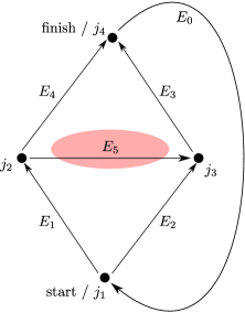
Figure 2: Schematic of Braess’ network with the edges $E_{0},\dots,E_{5}$ made up of TASEPs of length $L_{i}$ joined through junction sites $j_{1},\dots,j_{4}$. Edge $E_{5}$ is considered to be the new road which is added to the system, resulting in a newly available route from start to finish. Through $E_{0}$ periodic boundary conditions are achieved and the total number of particles $M$ is kept constant. The lengths of the TASEPs are chosen according to Eqs. (2) and (3) which according to Eqs. (4)-(6) results in route 153 being shorter than routes 14 and 23.

In the following, the systems without and with $E_{5}$ are also refered to as 4link and 5link system, respectively. Corresponding variables are marked with the superscripts ’$(4)$’ and ’$(5)$’. Since we want to compare how the systems with and without $E_{5}$ behave for the same demand $M$, we we introduce the two different global densities for the 4link and the 5link system as

$$\rho^{(4)}_{\text{global}} = M/\left(4+\sum_{i=0}^{4}L_{i}\right)$$ (7)

$$\rho^{(5)}_{\text{global}} = M/\left(4+\sum_{i=0}^{5}L_{i}\right)$$ (8)

$$= \frac{5+2L_{1}+2L_{2}}{2L_{2}+\frac{\hat{L}_{153}}{\hat{L}_{14}}(4+L_{1}+L_{2})}\rho^{(4)}_{\text{global}}.$$ (9)

The relation between the two different global densities for the same number of particles depends on $L_{5}$. The length $L_{5}$ can also be given by the pathlength ratio $\hat{L}_{153}/\hat{L}_{14}$, which describes how long the new route is compared to the old ones.

Each particle has a fixed strategy (or personal route choice) which does not change with time. Therefore the amounts of particles which take specific routes are the relevant free parameters in our system. For a fixed combination of the $L_{i}$ and $M$ the numbers of particles which use the different routes 14, 23 and 153 are given by $N_{14}$, $N_{23}$ and $N_{153}$. They are the tunable parameters in the system subject to the condition $N_{14}+N_{23}+N_{153}=M$. Specific choices of these numbers may drive the system into specific states. Useful quantities are

$$n_{\text{l}}^{(j_{1})} =1-\frac{N_{23}}{M},$$ (10)

$$n_{\text{l}}^{(j_{2})} =\frac{N_{14}}{N_{14}+N_{153}},$$ (11)

i.e. the fraction of particles which turn ’left’ on junctions $j_{1}$ and $j_{2}$, respectively. By varying $n_{\text{l}}^{(j_{1})}$ and $n_{\text{l}}^{(j_{2})}$ from 0 to 1, all possible combinations of $N_{14}$, $N_{23}$, $N_{153}$ and the corresponding values of certain observables we are interested in can be visualized in simple 2d-color-plots.

Fixing the individual strategies is a major difference to our previous work [1] on the Braess paradox. There the particles did not have individual strategies, but were all equal: particles sitting on junction sites $j_{1}$ or $j_{2}$ chose their routes according to the turning probabilities $\gamma$ and $\delta$, respectively. It is important not to confuse $n_{\text{l}}^{(j_{1})}$ and $n_{\text{l}}^{(j_{2})}$ with the turning probabilities $\gamma$ and $\delta$ in our previous article. The $n_{\text{l}}^{(j_{1}/j_{2})}$ are not turning probabilities for jumping left but they describe the fraction of particles jumping left on $j_{1}$/$j_{2}$ compared to the total number of particles. In the present paper the level of stochasticity is reduced to the random sequential update mechanism, whereas in [1], the turning probabilities were an additional source of stochasticity. As will be seen in Section 3, this difference leads to different characteristics in the system - in our context especially in the stability of measured travel time values as explained in detail for the 4link system in Section 3.1.

Networks comprised of TASEPs connected through junction sites and the route choice process governed by turning probabilities received a lot of research interest (see e.g. [19, 20, 21, 22]). In particular a network with a structure very similar to Braess’ network without $E_{5}$ was adressed in [23] in some detail. The case of networks with particles choosing routes according to personal strategies has to our knowledge not received as much attention.

Both the model with turning probabilities and the present model with fixed strategies can be regarded as realistic models of a commuter’s route choice scenario. Laboratory experiments in which humans repetitively had to perform route choices were performed in similar models with results suggesting that both fixed route choices or turning probabilities could be realistic. In [24, 25] a network similar to our network without $E_{5}$ and in [25] also the network with $E_{5}$ was examined. It turned out that in their aim to minimize their individual travel times, in the network without $E_{5}$ users kept varying their individual strategies while on average the strategies stayed the same. This is an indication that the model with turning probabilities is realistic. In the network with $E_{5}$, strategy changes of individual users seemed to vanish after some time rather indicating that the fixed-strategy model of the present paper is realistic. Therefore both models seem to have some validity and a mixture of both could be at play in reality. Before addressing this more complex scenario a good understanding of the differences between the two basic models seems to be helpful.

2.3 Possible network states

A state of the road network is given by a certain distribution of the particles onto the different routes, i.e. a certain combination of $N_{14}$, $N_{23}$ and $N_{153}$. A road network with selfish users is said to be in a stable state if the particles are distributed such that all used routes have the same travel time which is lower than that of any unused routes. Such a state is stable because it would not make sense for any particle to change its route since a potential change would result in an increase of the particle’s travel time. If drivers have knowledge of the current travel times of all routes, there is no incentive to alter their current route choice in a stable state. This state is also called the user optimum ($uo$) [6]. The user optimum is to be distinguished from the system optimum ($so$) which is the best state that can be reached from a global perspective. In the following we define the system optimum as the state which minimizes the maximum travel time in the system. This agrees with Braess’ choice in [4, 5]. Note that throughout the literature other definitions of the system optimum have been used, e.g. as the state minimizing the total travel time [26].

The system optimum is not necessarily stable for the case of selfish drivers [6]. In our analysis we want to compare the travel times in the user optima of the system without and with the new edge $E_{5}$. Generally, the system’s performance is improved by the addition of $E_{5}$ if the travel time in the user optimum of the system with $E_{5}$, i.e. the 5link system, is lower than that of the user optimum in the system without $E_{5}$, i.e. the 4link system. Braess’ paradox occurs, i.e. the system’s performance is decreased due to the new road, if the travel times in the user optimum of the system with $E_{5}$ are higher than the travel times in the user optimum of the system without $E_{5}$ [4, 5]. To gain a deeper understanding of the influence of $E_{5}$ on the system - beyond the question of the occurrence of Braess’ paradox - one can also compare the maximum travel times in the system optima of the 4link and the 5link system. The possible states are summarized in Figure 3.

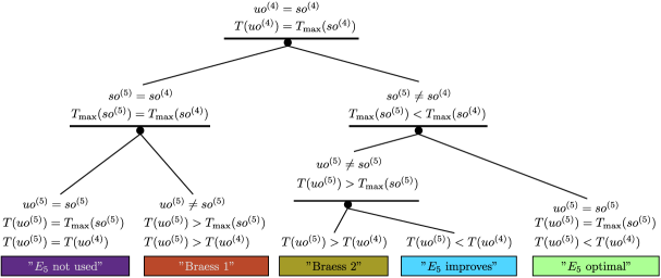
Figure 3: The possible states which can occur in our network. If the system optima of the 4link and the 5link system are equal the system performance cannot be improved due to $E_{5}$, it is either unchanged (”$E_{5}$ not used”) or rendered worse (”Braess 1”). If the system optima are unequal, then the 5link system optimum necessarily has a lower travel time than the 4link system optimum. Here, the system perfomance can be rendered worse (”Braess 2”) or be improved (”$E_{5}$ improves” and ”$E_{5}$ optimal”).

If the system optima are the same (left branch of the tree in Fig. 3), the system cannot be improved, even for the case of non-selfish drivers or with traffic guidance systems. If selfish drivers lead the 5link system into its optimum ($uo^{(5)}=so^{(5)}$) the new road will not be used at all (”$E_{5}$ not used”). If this is not the case, the new road will be used, but the travel times will increase (”Braess 1”). If the system optima of the 4link and the 5link are not the same, the system can potentially be improved (right branch of the tree in Fig. 3). Since the 4link system is included in the 5link system, the maximum travel time of the system optimum in the 5link system can only be smaller than that of the 4link system ($T_{\text{max}}(so^{(5)})<T_{\text{max}}(so^{(4)})$). If there is a traffic guidance system, the system can always always be improved. For selfish drivers and without such a system, if the 5link system does not reach its optimal state ($uo^{(5)}\neq so^{(5)}$), the system’s travel times in the user optimum can either be increased (”Braess 2”) or decreased (”$E_{5}$ improves”) due to the addition of $E_{5}$. If the 5link system reaches its optimum ($uo^{(5)}=so^{(5)}$), the system is said to be in the ”$E_{5}$ optimal” state.

The ”$E_{5}$ improves” and ”$E_{5}$ optimal” states are the only cases in which the new route is useful for the case of selfish drivers. In the ”Braess 2” case, the new road can be useful, if the system is driven into its system optimum by an external traffic guidance system but is not useful if the network is used by selfish drivers. In the other two phases, the new road has no effect or even renders the situation worse.

For this distinction between the possible states (or phases) it is essential to define the system optimum as the state that minimizes the maximum travel time. For different definitions, as e.g. the state maximizing the flow or the state minimizing the total travel time, this classification scheme does not necessarily hold.

If the user optima and system optima of the systems with and without $E_{5}$ can be found for all different length ratios $\hat{L}_{153}/\hat{L}_{14}$ and all different global densities, the full phase diagram can be constructed according to this classification scheme. In [1] this was done for the same network, but with turning probabilities instead of fixed amounts of particles choosing the different routes. In that analysis, the phases ”Braess 1”, ”$E_{5}$ improves”, ”$E_{5}$ optimal” and an additional domain wall phase were found.

2.4 Gridlocks

As described in Section 2.3 a state of the network is determined by strategy distributions as given by $N_{14},~{}N_{23},~{}N_{153}$ or $n_{\text{l}}^{(j_{1})},~{}n_{\text{l}}^{(j_{2})}$ (see Eqs. (10) and (11)). For certain combinations of $\hat{L}_{153}/\hat{L}_{14}$, $\rho^{(5)}_{\text{global}}$ and $N_{14},~{}N_{23},~{}N_{153}$ all sites of one path or of multiple paths can become completely occupied. This corresponds to a total gridlock of the whole system, since each route shares the sites $j_{1}$, $j_{4}$ and $E_{0}$. If one of the paths is gridlocked, the whole system is gridlocked. Once a gridlock developed it cannot dissolve, i.e. becomes a stationary state of the system. In an ergodic system (with finite edge lengths $E_{i}$) a possible gridlock state will always be reached at some point of the time evolution. In the following we describe under which circumstances gridlocks can occur.

In our simulations the system was always initialized such that particles were placed randomly but already on routes according to their strategies. E.g. a particle following strategy 14 could not be placed on $E_{2}$. The following arguments are based on this initialization strategy. When other strategies are used, e.g. completely random initial position irrespective of the strategy, more gridlocks can occur. A simple example for this are initial states where all sites on route 153 are occupied by the random initialization even if this is not possible according to the strategy distribution.

Gridlock on route 14

For the occurrence of a gridlock on route 14 the following three conditions must be met:

$$(N_{14}\geq L_{4}+1)~{}~{}~{}\land~{}~{}~{}(N_{14}+N_{153}\geq L_{1}+L_{4}+2)~{}~{}~{}\land~{}~{}~{}(M\geq\hat{L}_{14}=L_{1}+L_{4}+4).$$ (12)

The first condition $N_{14}\geq L_{4}+1$ is necessary since all sites on $E_{4}$ can only be occupied by particles of strategy 14. For a gridlock to occur, additionally to all sites on $E_{4}$, also junction $j_{2}$ must be occupied by a particle of the same strategy. As well as all sites of $E_{4}$ and $j_{2}$, also all sites on $E_{1}$ must be occupied at the same time. This can be by particles of strategies 14 or 153. Also junction $j_{1}$ must be occupied by a particle that wants to turn left, thus one of strategy 14 or 153. This is represented in the second condition $N_{14}+N_{153}\geq L_{1}+L_{4}+2$. For a complete gridlock of route 14, also sites $j_{4}$ and $E_{0}$ must be occupied. They can be be occupied by particles of any strategy 14, 153 or 23, which is represented in the third condition $M\geq\hat{L}_{14}$.

Gridlock on route 23

For the occurrence of a gridlock on route 23 the following three conditions must be met:

$$(N_{23}\geq L_{2}+1)~{}~{}~{}\land~{}~{}~{}(N_{23}+N_{153}\geq L_{3}+L_{2}+2)~{}~{}~{}\land~{}~{}~{}(M\geq\hat{L}_{23}=L_{3}+L_{2}+4).$$ (13)

The first condition $N_{23}\geq L_{2}+1$ is necessary since all sites on $E_{2}$ can only be occupied by particles of strategy 23. For a gridlock to occur, additionally to all sites on $E_{2}$, also junction $j_{1}$ must be occupied by a particle of the same strategy. As well as all sites of $E_{2}$ and $j_{1}$, also all sites on $E_{3}$ must be occupied at the same time. This can be by particles of strategies 23 or 153. Also junction $j_{3}$ must be occupied by one of those particles. This is represented in the second condition $N_{23}+N_{153}\geq L_{3}+L_{2}+2$. For a complete gridlock of route 23, also sites $j_{4}$ and $E_{0}$ must be occupied. They can be be occupied by particles of any strategy 14, 153 or 23, which is represented in the third condition $M\geq\hat{L}_{23}$.

Gridlock on route 153

The conditions for the occurrence of a gridlock on route 153 are a bit more complicated since there is edge $E_{5}$ which can only be used by particles of strategy 153 and there are the edges $E_{1}$ and $E_{3}$ which can be used by particles of strategies 153 and 14 and 153 and 23, respectively. The first condition which has to be met is

$$N_{153}\geq L_{5}+1.$$ (14)

This represents all sites of $E_{5}$ and junction $j_{2}$ being occupied by particles of strategy 153. Then one has to consider the remaining particles of strategy 153 which we denote by $r_{153}=N_{153}-L_{5}-1$. They can now be distributed onto edges $E_{1}$ and $E_{3}$. As the second condition for a gridlock possibility on route 153, there has to exist an integer number $a\in\mathbb{N}$ with $0\leq a\leq r_{153}$ such that

$$(r_{153}-a+N_{14}\geq L_{1}+1)~{}~{}~{}\land~{}~{}~{}(a+N_{23}\geq L_{3}+1).$$ (15)

The first part means that all sites on $E_{1}$ and also junction $j_{1}$ must be occupied by particles of strategies 14 or 153. The second one means that junction $j_{3}$ and all sites on $E_{3}$ must be occupied by particles of strategies 153 or 23. The third condition is

$$M\geq\hat{L}_{153}=L_{1}+L_{5}+L_{3}+5.$$ (16)

This ensures that sites $j_{4}$ and $E_{0}$ are occupied (by particles of any strategy 14, 23 or 153). Summarzing, for a gridlock on route 153 to be possible the conditions in (14) and (16) have to be met and an integer number $a\in[0,r_{153}]$ has to exist such that the two conditions in (15) can be fulfilled.

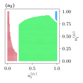
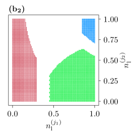
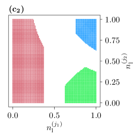
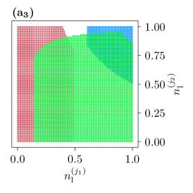
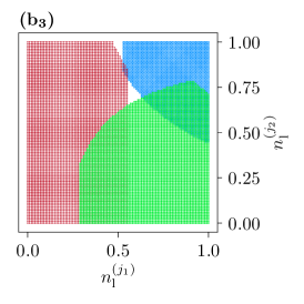
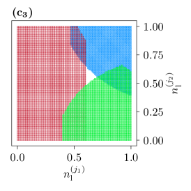
Figure 4: The $\left(n_{\text{l}}^{(j_{1})},~{}n_{\text{l}}^{(j_{2})}\right)$ - landscapes for $L_{1}=100$, $L_{2}=500$ and (a₁) $\hat{L}_{153}/\hat{L}_{14}=0.4$ and $\rho^{(5)}_{\text{global}}=0.2$, (a₂) $\hat{L}_{153}/\hat{L}_{14}=0.4$ and $\rho^{(5)}_{\text{global}}=0.5$, (a₃) $\hat{L}_{153}/\hat{L}_{14}=0.4$ and $\rho^{(5)}_{\text{global}}=0.8$, (b₁) $\hat{L}_{153}/\hat{L}_{14}=0.7$ and $\rho^{(5)}_{\text{global}}=0.2$, (b₂) $\hat{L}_{153}/\hat{L}_{14}=0.7$ and $\rho^{(5)}_{\text{global}}=0.5$, (b₃) $\hat{L}_{153}/\hat{L}_{14}=0.7$ and $\rho^{(5)}_{\text{global}}=0.8$, (c₁) $\hat{L}_{153}/\hat{L}_{14}=1.0$ and $\rho^{(5)}_{\text{global}}=0.2$, (c₂) $\hat{L}_{153}/\hat{L}_{14}=1.0$ and $\rho^{(5)}_{\text{global}}=0.5$, (c₃) $\hat{L}_{153}/\hat{L}_{14}=1.0$ and $\rho^{(5)}_{\text{global}}=0.8$. The landscapes were discretized in steps of 0.01. States with a gridlock possibility on routes 14, 23 and 153 are marked with blue $\times$’s, red $+$’s and green $\star$’s respectively.

Figure 4 shows for which points in the $\left(n_{\text{l}}^{(j_{1})},~{}n_{\text{l}}^{(j_{2})}\right)$ - landscape (i.e. the phase space of the system) gridlocks on the routes are possible for several combinations of $\hat{L}_{153}/\hat{L}_{14}$ and $\rho^{(5)}_{\text{global}}$. One can see that with growing global density more and more strategies can become gridlocked. One can also see that depending on the length ratio between the new route and the old routes, different strategies can become gridlocked. For low values of $\hat{L}_{153}/\hat{L}_{14}$ more strategies with high $n_{\text{l}}^{(j_{1})}$ and low $n_{\text{l}}^{(j_{2})}$ lead to a gridlock on route 153 which makes sense since the new route is much shorter compared to the old ones. For longer $L_{5}$, thus higher $\hat{L}_{153}/\hat{L}_{14}$, routes 14 and 23 are becoming more and more likely to be gridlocked as well.

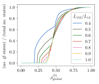
Figure 5: The number of states with gridlock probabilities over the total number of states against the global density $\rho^{(5)}_{\text{global}}$ for different values of $\hat{L}_{153}/\hat{L}_{14}$. To calculate the ratio the $\left(n_{\text{l}}^{(j_{1})},~{}n_{\text{l}}^{(j_{2})}\right)$ - landscapes were discretized in steps of 0.01 and the number of states with gridlock possibility were counted and then divided by the total number of states.

In Figure 5 the ratio of the number of states with gridlock possibility over the total number of states is shown against the global density for various pathlength ratios for $L_{1}=100$ and $L_{2}=500$. To obtain this plot, the $\left(n_{\text{l}}^{(j_{1})},~{}n_{\text{l}}^{(j_{2})}\right)$ - landscapes were discretized in steps of 0.01 and the number of states with gridlock possibility were counted. Since in our case $\hat{L}_{153}$ is always smaller than $\hat{L}_{14}=\hat{L}_{23}$, the lowest density with a gridlock probabiliy is always the density with $M=\hat{L}_{153}$ (cf. Eq. (16)). One can see that for lower values of $L_{5}$ a large region of the phase space is comprised of states with gridlock probabilities even for low densities (e.g. over 60% of states can become gridlocked at densities of $\rho^{(5)}_{\text{global}}\approx 0.4$ for $\hat{L}_{153}/\hat{L}_{14}=0.4$). For longer $E_{5}$ less states can become gridlocked. Please note that this figure depends on how fine the discretization of space is chosen and also on how phase space is desribed. It might look different if the phase space is chosen to be three-dimensional and described by $(N_{14},~{}N_{23},~{}N_{153})$ instead of $\left(n_{\text{l}}^{(j_{1})},~{}n_{\text{l}}^{(j_{2})}\right)$. When a gridlock state will occur in the system may depend on the individual realization of the stochastic process. A closer look at when gridlocked states occur is given in Section 3.2.2.

2.5 Monte-Carlo observables

We analysed the system by employing Monte Carlo (MC) simulations. Details of the measurement processes can be found in A. In a first step, the system and user optima were found by analysing the values of the two observables

$$\Delta T = |T_{14}-T_{23}|+|T_{14}-T_{153}|+|T_{23}-T_{153}|,$$ (17)

$$T_{\text{max}} = \text{max}[T_{i},i\in\{14,23,153\}].$$ (18)

$T_{i}$ denotes the travel time on route $i$, i.e. the time a particle needs to go from $j_{1}$ to $j_{4}$ via this route. The user optima and system optima are given by the combinations of $N_{14}$, $N_{23}$, $N_{153}$ (or $n_{\text{l}}^{(j_{1})}$ and $n_{\text{l}}^{(j_{2})}$) which minimize $\Delta T$ and $T_{\text{max}}$, respectively.

A true user optimum is characterized by $\Delta T(n_{\text{l}}^{(j_{1})},n_{\text{l}}^{(j_{2})})=0$ since then all routes have the same travel times. If there are any unused routes and the travel times of these unused routes are higher than that of the used ones, $\Delta T$ is reduced to only the absolute values of the travel time difference of the used routes (see B for an example of this case). In our simulations, a strategy with a $\Delta T$ value close to zero is regarded as a user optimum since the exact zero case is seldom found when measuring travel times.

The system optimum is given by the strategy which minimizes $T_{\text{max}}$. By comparing the positions and travel time values of the user and system optima of the 4link and 5link systems, the phase diagram can be constructed according to the scheme described in Section 2.3. If a true user optimum is found, all three routes have the same travel time. In this case this travel time can be compared to the maximum travel time of the system optimum. In cases where we could not find exact user optima, we compared the maximum travel time of the ’closest candidate’ for the user optimum (state with lowest $\Delta T$) to the maximum travel time of the system optimum. More details on the cases where no real user optima could be found are given in Section 3.2.2.

3 Results

3.1 Travel times in the 4link network

Since the 4link system, our reference system, is symmetric one expects the user optimum and the system optimum to be given by half the particles taking route 14 and the other half taking route 23 for all possible global densities $\rho_{\text{global}}^{(4)}$. In Fig. 6 we can see that this is indeed the case.

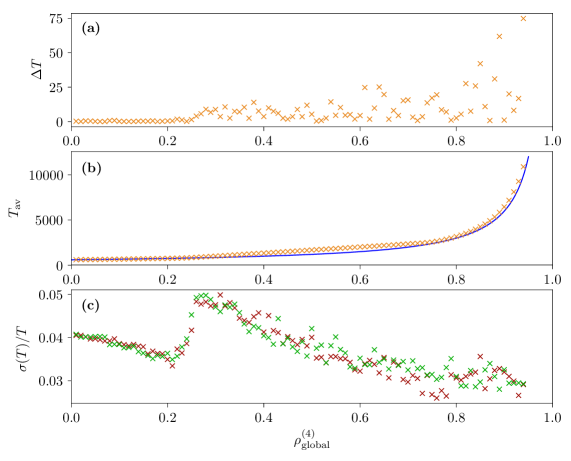
Figure 6: Results of MC simulations of the 4link system for 50% of the particles choosing route 14 and 50% choosing route 23 for the whole density regime $0\leq\rho_{\text{global}}^{(4)}\leq 1$ and $L_{1}=L_{3}=100$ and $L_{2}=L_{4}=500$. Part (a) shows, that throughout all densities, the travel times on routes 14 and 23 are almost equal. Part (b) shows the average travel times on these routes (orange $\times$’s) and for comparison the travel time of a single TASEP with $M/2$ particles according to Equation (1) (blue line). One can see, that jamming at $j_{4}$ plays an important role for densities $\rho_{\text{global}}^{(4)}\gtrsim 0.2$. As can be seen in part (c), the relative standard deviations of the travel times on both routes are below $5\%$ for all densities (values for route 14/23 in red/green.

In Figure 6 (a) we see the value of $\Delta T=|T_{14}-T_{23}|$ (Equation (17) reduces to this form in the 4link system) against the global density. The value is close to zero for all global densities which means that the travel times are (almost) equal on both routes and this symmetric distribution of the particles is indeed the user optimum. Since the network is symmetric, this is also the system optimum, as any unequal distribution of the particles would lead to a higher travel time on the route with more particles.

In Figure 6(b) the average of the travel times measured on routes 14 and 23 ($T_{av}=(T_{14}+T_{23})/2$) is shown. For comparison also the travel time of a single TASEP used by $M/2$ particles (obeying Equation (1)) is indicated by the blue line. One can see that for densities $\rho_{\text{global}}^{(4)}\gtrsim 0.2$ the jamming at $j_{4}$ plays an important role since the travel times are higher than those of the single TASEP from this density upwards.

In Figure 6(c) we can see the relative standard deviation of the travel time measurements of both routes

$$\sigma(T)/T=\frac{1}{\bar{T}}\left(\frac{1}{n}\sum_{i=1}^{n}(T_{i}-\bar{T})^{2}\right)^{1/2}$$ (19)

with $n$ being the number of measurements and

$$\bar{T}=T=\frac{1}{n}\sum_{i=1}^{n}T_{i}$$ (20)

being the mean of all measured values. One can see that it stays below $5\%$ for all densities. This means we measure stable travel time values for all densities which is also supported by the measured density profiles (Figure 7). They show a sharp domain wall between low and high density regions at a fixed position which is the same on both routes.

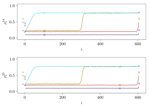
Figure 7: Density profiles of the two routes in the 4link system with $L_{1}=L_{3}=100$ and $L_{2}=L_{4}=500$ for the four different global densities $\rho_{\text{global}}^{(4)}\in\{0.1,0.2,0.5,0.75\}$ printed in $\{$purple, orange, brown, blue$\}$. The local densities $\rho_{i}^{14/23}$ on the two routes are shown against the position $i$. The denisity on $E_{0}$ is given by a $+$, the density of junction sites on the roads by $\times$’s. One can see that in all cases the density profiles are almost equal on both routes. Domains walls form at the same fixed positions on both routes.

This is a very important difference to the model with higher stochasticity due to turning probabilities [1]. In the more stochastic case, fluctuating domain walls dominate the density region $0.29\lesssim\rho^{(4)}_{\text{global}}\lesssim 0.75$ resulting in (short-term) unstable travel time values. A comparison of the different behaviours of the two models is shown in Figure 8.

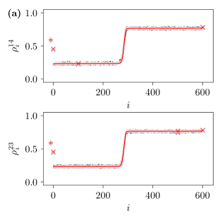
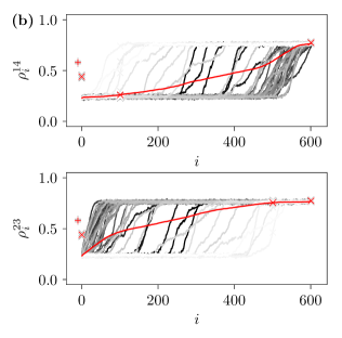
Figure 8: A comparison of the density profiles of routes 14 and 23 in the 4link systems with $L_{1}=L_{3}=100$ and $L_{2}=L_{4}=500$ and $M=622$, $\rho_{\text{global}}^{(4)}\approx 0.52$ in the present less stochastic model (part (a)) and in the model with higher stochasticity (with turning probability $\gamma=0.5$) treated in our previous article [1] (part (b)). In both parts, the averaged density profiles over the whole measurement time of $10^{6}$ sweeps is shown in red and 50 different shortterm instances (averaged over $10^{4}$ sweeps each) are shown in 50 different shades of gray. The density on $E_{0}$ is given by a $+$, the density of junction sites on the roads by $\times$’s. One can see that in the present model, the domain wall position is fixed, while it fluctuates through the routes in a coupled manner in the model with higher stochasticity.

In Fig. 8 (a) and (b) density profiles of the present model and of that treated in [1] are shown. The averaged density profiles measured over the whole measurement time of $10^{6}$ sweeps are given in red. In different shades of gray, different measurement instances (averaged over $10^{4}$ sweeps each) are shown. As one can see in part (a) of the figure, in the present model the domain wall is at the same fixed position during the whole measurement process: all the grey curves lie below the red curve. In the model with turning probabilities this is not the case as seen in part (b). Here, the averaged density profile becomes close to a straight ascending line on both paths. This is due to the fact that the domain walls perform a coupled random walk on the two paths. If the high density region gets longer on one path it gets shorter on the other one respectively. The domain wall positions can be at any point of the paths depending on the measurement time. Therefore, particles entering the same route at different times may encounter a completely different situation and thus have completely different travel times even if the system is in its stationary state and none of the parameters changes. This behaviour of the model with higher stochasticity is treated in detail in [1].

Due to the fluctuating domain walls and the resulting unstable travel times in the model with higher stochasticity $uo$ and $so$ could not be determined in a large intermediate global density region. Thus the system’s reaction to the addition of $E_{5}$ could not be classified according to our scheme presented in Section 2.3 in this density region. In the present case we obtain stable travel time values and thus $uo$ and $so$ throughout the whole density region for the 4link system. Thus we are able to compare the 5link system to the 4link system in the whole density region.

3.2 Phase diagram

We used Monte Carlo simulations to obtain the user optima and system optima of the 5link system for different combinations of $L_{5}$ and $M$. States with potential gridlock formation as explained in Section 2.4 were not considered as candidates for user or system optima. Even if some of these states may, depending on the initial configuration and realization of the stochastic process, have values of $\Delta T$ close to zero in the beginning of the system’s time evolution, they all evolve into a gridlock steady state (more details on this in Sec. 3.2.2). By comparing the travel times of the found 5link user and system optima to those of the 4link system’s user and system optima for the same $M$ we could derive the phase diagram of the system according to the classification shown in Figure 3. In A we describe our procedure to find the user and system optima in more detail. The phase diagram (Fig. 9) and the following Fig. 12 show the influence of the control parameters $L_{5}$ and $M$: The $x$-axis is always given by $\hat{L}_{153}/\hat{L}_{14}$ which is the ratio of the lengths of the new route 153 and the two old routes 14 and 23 (see Eqs. (4) – (6)). There are always two $y$-axes which decode the number of particles $M$ via the global densities in the 4link/5link systems $\rho_{\mathrm{global}}^{(4)/(5)}$ (see Eqs. (7) – (9)).

3.2.1 Phase diagram’s structure

The phase diagram shown in Figure 9 (a) can be divided into three parts.

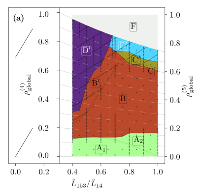
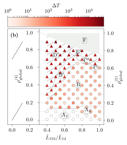
Figure 9: The shown results were obtained for $L_{1}=L_{3}=100$, $L_{2}=L_{4}=500$ and varying lengths of $E_{5}$ (resulting in the x-axis $\hat{L}_{153}/\hat{L}_{14}$) and $M$ (resulting in the two y-axes $\rho_{\mathrm{global}}^{(4)/(5)}$). (a) The phase diagram according to the classification scheme given in Figure 3. The $\times$’s show where simulations were performed. The phase boundaries are drawn according to those simulations and are thus, due to this limited number of simulations, only a rough estimate of the phase boundaries. In phases A, B and C real user optima could by found while in the area marked by a hatching (phases B^′, C^′, D^′, E^′) no real user optima could be found. In phase F the 4link system is full. (b) The value of $\Delta T$ for selected measurement points. One can see that it is below 100 (indicated by coloured $\bigcirc$) in the unhatched area and above 100 (indicated by coloured $\bigtriangleup$) in the hatched area.

The trivial first part is called phase F. This phase is present for really high densities in the 5link system. In this phase, there are more particles in the 5link system than sites in the 4link system. The 4link system is thus completely blocked and the two systems cannot be compared. One could argue that $E_{5}$ improves the system at these high densities, but only in the sense that the 4link could not even take up that many particles.

The second part, consisting of phases A_1/2, B and C, is the part in which real user optima of both the 4link and the 5link system exist in the sense that states in which $\Delta T\approx 0$ exist, i.e. states with almost equal travel times on all three routes.

The third part is given by the region above the light dotted line which is marked by a hatching and consists of the ”primed” phases B^′, C^′, D^′ and E^′. In all of these phases no real user optima exist in the sense that no states with $\Delta T<100$ could be identified. This means that in neither of these phases a distribution of the particles onto the routes exists which leads to (almost) equal travel times on all routes. This is a consequence of gridlocked states: Combinations of $n_{\text{l}}^{(j_{1})}$ and $n_{\text{l}}^{(j_{2})}$ which would potentially be a user optimum are not available since they would lead to a gridlock.

The values of $\Delta T$ in some points of the phase diagram are shown in Figure 9 (b). As can be seen, in phases A, B and C the value is zero or of the magnitude of 10, while it is higher than 100 in the hatched phase, reaching up to values of the order of $10^{4}$ at really high densities.

Phases A_1/2 are ”$E_{5}$ optimal” phases. In these phases, the travel times in the $uo$ of the 5link system are lower than that of the $uo$ in the 4link system and $uo^{(5)}=so^{(5)}$. In phase A₁, the region below the dotted line at low path length ratios and low global densities, the $uo$ of the 5link is given by all particles choosing route 153. The new route is the only used route of the system. In phase A₂, above the dotted line, all three routes are used in the 5link user optima.

Phase B is the ”Braess 1” phase. Here the $so$ of the 5link is equal to that of the 4link, meaning half of the particles choose route 14 and the other half route 23. The user optimum of the 5link is given by another distribution of particles onto the three routes, such that all three routes have the same higher travel time. The ”Braess 1” phase actually dominates the largest part of the phase diagram. There is also a very small part of the phase diagram at densities around $\rho_{\mathrm{global}}^{(4)}\approx 0.8$ and $\hat{L}_{153}/\hat{L}_{14}\gtrsim 0.7$, in which the ”Braess 2” phase (phase C) is found, meaning that with traffic regulations the system could be improved due to $E_{5}$ ($T_{\mathrm{max}}(so^{(5)})<T_{\mathrm{max}}(so^{(4)})$), but without regulations - in the $uo$ - the travel times are increased due to the addition of $E_{5}$.

In the hatched area, in the 5link system no real user optima with equal travel times on all routes exist. This is because combinations of $n_{\text{l}}^{(j_{1})}$ and $n_{\text{l}}^{(j_{2})}$ which could potentially lead to equal travel times on all routes lead to gridlocks in the system according to Section 2.4. Only states without the possibility of a gridlock were taken into account for the construction of the phase diagram. In most cases, the state with the lowest value of $\Delta T$ and without gridlock possibility is a state in which the travel time on route 153 is lower than on the other two. When more particles choose route 153, $T_{153}$ increases. But before a state with equal travel times on all routes is reached, route 153 and subsequently all three routes come to a complete gridlock. More details on the hatched area and an illustrative example can be found in Section 3.2.2.

For the construction of our phase diagram we used the state with the lowest value of $\Delta T$ and without gridlock possibility we could find and compared its maximum travel time to that of the system optimum and the user optimum of the 4link system. It is important to keep in mind that even though in this manner we could identify different phases inside the hatched region, there are no real user optima in the 5link in all of the primed phases. In a system with real drivers more and more drivers would tend to switch routes with the desire to reduce their own travel time and in the long run the system will evolve into a complete gridlock.

Here, judging from the maximum travel times in the state with the lowest $\Delta T$, we could identify two phases in which the system could not be improved even if the traffic was externally regulated. These are the ”$E_{5}$ not used - like” phase (phase A^′) and the a ”Braess 1 - like” phase (phase B^′). In both of those phases the $so$ of the 5link equals that of the 4link. While in the former this is also the state with the lowest value of $\Delta T$ (and real drivers would thus tend to switch to route 153), in the second one another state with a higher maximum travel time gives the lowest value of $\Delta T$. In the ”Braess 2 - like” phase (phase C^′) the system could be improved by the addition of $E_{5}$ if the traffic is regulated but is not for selfish drivers. In the ”$E_{5}$ improves - like” phase (phase E^′), the maximum travel time in the state with the lowest $\Delta T$ in the 5link is lower than that of the 4link but is not as low as in the 5link’s system optimum.

Summarizing we can conclude that in a system of selfish drivers without traffic regulations the addition of $E_{5}$ only reduces travel times at low densities $\rho_{\mathrm{global}}^{(5)}\lesssim 0.2$ (phases A_1/2). Here the system with the new road will also be in its optimal state ($uo^{(5)}=so^{(5)}$). At really high densities, the system shows ”$E_{5}$ improves - like” behaviour (phase E^′), meaning that in the 5link system the state in which all three travel times are closest to each other has a lower maximum travel time than the user optimum of the 4link system. Still the 5link is not in its optimum in this state and, more importantly, this is not a real user optimum. Instead the system is prone to gridlocks when used by real drivers since more and more of them would tend to choose route 153. In most parts of the system, the addition of $E_{5}$ leads to higher travel times in the system used by selfish drivers (phases B, B^′, C^′) or the new road will be ignored (phase D^′). In most of these phases (phases B, B^′, D^′) even if external traffic guidance was applied, $E_{5}$ would not reduce travel times.

3.2.2 The region without proper user optima

Here we take a closer look at the phases in the area of the phase diagram which is marked by a hatching (Figure 9) by analysing an exemplary point of this region: we look at the point with the parameters $\hat{L}_{153}/\hat{L}_{14}=0.5$ and $\rho_{\mathrm{global}}^{(5)}=0.49$. According to the phase diagram shown in Fig. 9 this is a point of the B^′ phase (”Braess1 - like” phase). In Fig. 10 we show the $n_{\text{l}}^{(j_{1}/j_{2})}$ - landscapes and the corresponding $\Delta T$ and $T_{\mathrm{max}}$ values. In Fig. 10 certain points are marked and the corresponding travel time values of the three paths and the $\Delta T$ and $T_{\mathrm{max}}$ values for these points are shown in Table 1.

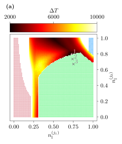
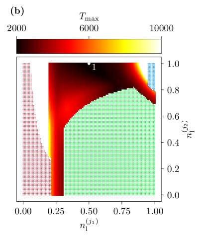
Figure 10: The $n_{\text{l}}^{(j_{1}/j_{2})}$ - landscapes of (a) the $\Delta T$ and (b) the $T_{\mathrm{max}}$ -values for $L_{5}=97$ and $M=638$, which means $\hat{L}_{153}/\hat{L}_{14}=0.5$ and $\rho_{\mathrm{global}}^{(5)}=0.49$. States with a gridlock possibility on routes 14, 23 and 153 are marked with blue $\times$’s, red $+$’s and green $\star$’s respectively. Simulations were performed for regions where no gridlock is possible and $n_{\text{l}}^{(j_{1}/j_{2})}$ was sweeped in steps of 0.01. The pink point $+1$ is the point with the lowest value of $\Delta T$. Thus this is the point which is used for the phase diagram. The grey points $+2$ and $+3$ have smaller values of $\Delta T$ but route 153 can gridlock. The white point $\star 1$ has the lowest value of $T_{\mathrm{max}}$ and is thus the system optimum.

In part (b) of Fig. 10 the point $\star 1$ represents the system optimum of this parameter set. It is given by half the particles choosing route 14 and the other half route 23. This point has the lowest value of $T_{\mathrm{max}}=1789$. It is not the user optimum as it has a high value of $\Delta T=2230$ since the travel time on route 153 is much lower than on the other routes. More and more particles would tend to switch to route 153. The point $+1$ shown in Fig. 10 (a) is the point which we used for our construction of the phase diagram. It is the point with the lowest value of $\Delta T=2215$ of all the points without gridlock possibility. From Table 1 we see that at this point route 153 still has a much lower travel time than the routes 14 and 23. In a system with real selfish drivers, more and more drivers would thus switch onto route 153.

Table 1: The $n_{\text{l}}^{(j_{1}/j_{2})}$, $\Delta T$, $T_{\mathrm{max}}$ and travel time values of the routes for the 4 points which are marked in Figure 10 (a) and  (b). Point $+1$ is the point with the lowest value for $\Delta T$ without a gridlock possibility. Thus this is the point we chose for construction of the phase diagram. Point $\star 1$ is the system optimum. The points $\times 1$ and $\times 2$ are states with gridlock possibilities on route 153. The measured travel time values are marked with a star because they were measured before the system gridlocked and are not stationary state values.

Point	$n_{\text{l}}^{(j_{1})}$	$n_{\text{l}}^{(j_{2})}$	$T_{14}$	$T_{23}$	$T_{153}$	$\Delta T$	$T_{\mathrm{max}}$
$+1$	0.730	0.798	2270	2047	1162	2215	2270
$\times 2$	0.741	0.735	2113⋆	2015⋆	1539⋆	1148⋆	2113⋆
$\times 3$	0.752	0.671	2797⋆	2744⋆	2748⋆	106⋆	2797⋆
$\star 1$	0.5	1.0	1789	1789	674	2230	1789

From Figure 10 (a) we know that if more particles choose route 153, a gridlock on that route becomes possible. We marked two more points (point $\times 1$ and $\times 2$) in this figure. From Table 1 we see that the value of $\Delta T$ decreases for those two points. It is important to keep in mind though that the travel time values of points $\times 1$ and $\times 2$ were measured before the system gridlocked. In Figure 11 we see how travel times of the individual routes and the value of $\Delta T$ develop during the measurement process at point $\times 3$.

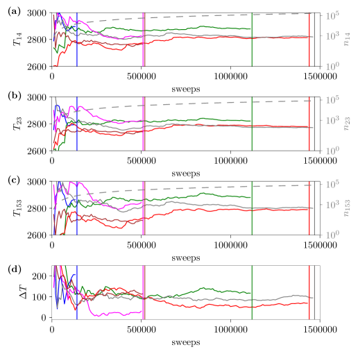
Figure 11: The time evolution of (a) - (c) the measured mean values of the travel times of the three routes and (d) the value of $\Delta T$ for the state $\times 3$ shown in Figure 10. The different coloured curves show six different instances of the system realized with six different seed values for the random number generator. The second y-axes on the right sides of the first three figures show how many times $n_{i}$ the values of $T_{i}$ were measured, represented by the dotted grey line. The vertical lines show the points in time when the system gridlocked on route 153.

For this figure six instances of the system with different seed values for the random number generator were generated and the travel times were measured during the evolution of the system. The system was not relaxed before measurements begun (the system was always relaxed for all measurements which were used for the phase diagram though - compare A for details on our general measurement process). The relaxation was skipped here since otherwise the system may have already gridlocked during the relaxation process. One can see that the state $\times 3$ is actually a good candidate for a user optimum since the value of $\Delta T$ seems to be very low since all three routes have similar travel times (also compare Table 1 for the numbers). All six instances of the system gridlock at some point of the time evolution. The earliest gridlock occurs after 130000 sweeps (blue line) and the latest after 1470000 sweeps (grey line). This example shows rather clearly that in the hatched area of the phase diagram, if the system was actually used by intelligent selfish particles, the gridlock possibility is very high. This is because states with gridlock possibilities have actually lower possible values of $\Delta T$. Thus more and more particles would tend to switch routes with the aim of reducing their own travel times but with the risk of causing a gridlock of the whole network. This is why for our phase diagram (Figure 9) and for our further analysis on the influence of $E_{5}$ on the system (see Sec. 3.2.3 and Fig. 12 therein) we only considered points without gridlock possibility and measured the travel time values of the steady states.

3.2.3 A closer look at the influence of the new edge

When talking about the Braess paradox, foremost one is interested in the relation of the travel times of the user optima of a road network before and after adding a new road. In Figures 12 (a) to (c), our two systems are studied in a bit more detail by comparing $so^{(5)}$ to $so^{(4)}$, $so^{(5)}$ to $uo^{(5)}$ and finally $uo^{(5)}$ to $uo^{(4)}$. Note that in parts (a) and (b) of the figure, the values used for $T_{\mathrm{max}}(so^{(5)})$ may actually not be the absolutely lowest possible maximum travel times. This is due to the fact that, opposed to the value of $\Delta T$ going to zero in the user optimum, a natural lower bound for $T_{\mathrm{max}}$ does not exist. Therefore one cannot be sure if the actual system optimum was found precisely (for more details, see A.2). Furthermore it is not guaranteed that we found all possible user optima and therefore the values (given by the colors) should be interpreted as tendencies of how the new road influences the system and not as exact values (see B for details - in some cases actually multiple $uo$s were found).

In Figure 12 (a) additionally to the underlying phase structure, for some specific points, the ratio of the system optimum’s maximum travel time in the 5link system and that of the 4link system $T_{\text{max}}(so^{(5)})/T_{\text{max}}(so^{(4)})$ is shown.

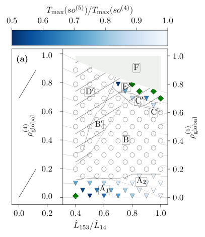
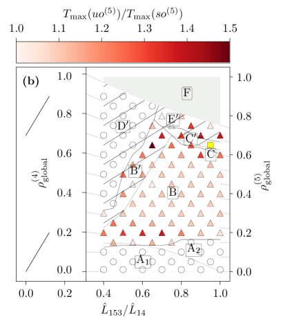
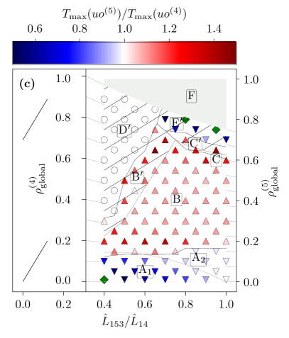
Figure 12: Quantifications of the influence of $E_{5}$ on the network. In all three parts, white $\bigcirc$ indicate values equal to 1, coloured $\bigtriangleup$ indicate values between 1 and 1.5, coloured $\bigtriangledown$ indicate values between 0.5 and 1, green $\diamondsuit$ indicate values below 0.5 and yellow $\Box$ indicate values above 1.5. Part (a) shows how the new road could improve the system if it was always in its system optimum, measured by $T_{\text{max}}(so^{(5)})/T_{\text{max}}(so^{(5)})$. Part (b) measures the so-called price of anarchy given by $T_{\text{max}}(uo^{(5)})/T_{\text{max}}(so^{(5)})$. This measure explains how much the travel times go up in the 5link, if users are selfish and not guided by external measures. Part (c) shows how much the travel times go up/down due to $E_{5}$ compared to the 4link system if the network is used by selfish drivers, measured by $T_{\text{max}}(uo^{(5)})/T_{\text{max}}(uo^{(4)})$.

In the 4link, the system optimum equals the user optimum and is thus reached by selfish drivers without any traffic guidance. In the 5link system, for selfish drivers the system optimum is only reached in the $E_{5}$ optimal phase (phases A_1/2). In the other phases, the system optimum would only be reached by forcing specific amounts of particles to choose specific routes via some traffic guidance system. In this case the system optimum could be reached everywhere. Figure 12 (a) shows us these potential benefits of route $E_{5}$. Since phase B (and B^′) is a ”Braess 1” phase and phase D^′ a ”$E_{5}$ not used-like” phase, here the system optima of 4link and 5link are equal and thus the ratio is 1. In this large phase space region the new road cannot have any positive effect - even if traffic is guided. The potential positive effect of $E_{5}$ is largest for low global densities and low values of $\hat{L}_{153}/\hat{L}_{14}$ (phase A₁) and for really high global densities (phase E^′). In the first case, actually all cars would use the new route and this would also be achieved without traffic guidance since in this phase $uo^{(5)}=so^{(5)}$. The ratio $T_{\text{max}}(so^{(5)})/T_{\text{max}}(so^{(4)})$ takes values as low as 1/2 meaning that the $so$ travel time can be reduced by 1/2. In phase E^′, the new route brings high benefits, since the 4link system here is almost full and thus travel times in the 4link rapidly diverge (see Figure 6 (b)). Here the increased capacity due to $E_{5}$ leads to high potential benefits, $T_{\text{max}}(so^{(5)})/T_{\text{max}}(so^{(4)})$ takes values smaller than 1/2. These full benefits would only be achieved by traffic guidance in this case, since here $uo^{(5)}\neq so^{(5)}$.

In Figure 12 (b) the so-called price of anarchy [27] inside the 5link system given by the ratio of $T_{\text{max}}(uo^{(5)})/T_{\text{max}}(so^{(5)})$ is shown. The price of anarchy is the ratio of the maximum travel time in the user optimum (in phases A, B, C real $uo$ exist and thus all travel times are almost equal in those $uo$) and the maximum travel time in the system optimum $T_{\text{max}}(uo^{(5)})/T_{\text{max}}(so^{(5)})$. In the 4link system it is always equal to 1 since the user optimum equals the system optimum. As already shown in Figure 3, in the 5link system it is always greater or equal to 1. In phases A_1/2, the ’$E_{5}$ optimal’ phases, it is obviously equal to 1. In phase B, it is higher than 1 with values around 1.3. Not routing the traffic externally becomes really costly at high densities in the 5link system. Here the maximum travel times in the user optimum are in some cases more than 1.5 times larger than those of the system optimum.

In Figure 12 (c) the ratio of the travel times in the user optima of the 4link and 5link systems $T_{\text{max}}(uo^{(5)})/T_{\text{max}}(uo^{(4)})$ is shown. This is the situation that the original Braess paradox deals with: how do the user optimum travel times in a system with selfish drivers change due to the additional road. The new road is in the case of selfish drivers only beneficial at low global densities and really high global densities. In the ”Braess 1” phase (phase B) it takes values of approximately $1.2-1.4$ and the travel time is increased by this factor due to $E_{5}$.

4 Conclusion

We analysed Braess’ network with TASEP dynamics on the edges considering periodic boundary conditions and individual drivers following fixed individual strategies. Different to the case of identical particles controlled by turning probabilities at the junction sites [1] we could find stable travel times throughout the whole density region of both the network with and without the new edge. Without the new road, system and user optima could be found for all densities. In the major part of the phase space real user optima could also be identified in the system with the new road. Only if the new route resulting from the new road is really short compared to the old routes or the global density is really high, no real user optima exist.

In the phase space region where real user optima exist, the new road leads to lower travel times only at low global densities $0\leq\rho_{\mathrm{global}}^{(4)/(5)}\lesssim 0.2$. The largest part of the phase space is dominated by the Braess phases, with the ”Braess 1” phase being the most prominent phase. The ”Braess 2” phase is also found in a small phase space region.

At high global densities or small path lengths of the new path no real user optima exist. This is due to the fact that here the system is prone to gridlock completely if all particles try to reduce their travel times. In this region of the phase space we chose the closest candidate of a user optimum without a possibility of gridlocks to construct the phase diagram. It turns out that here the new road also leads to higher travel times in most situations or is even completely ignored. Only at really high densities the road leads to lower travel times. Still in this whole region the system is at risk of gridlocks. This gridlock risk is also a consequence of added periodic boundary conditions and could vanish if the system was treated with open boundaries and a sufficiently large exit probability.

Additionally to constructing the phase diagram we could quantify how the new road influences the system for selfish users and also what would happen if an external travel guidance authority would drive the system into its system optimum. Even if traffic was guided the network’s performance, in terms of tavel times, would only be improved at really high or really low densities. The price of anarchy is relatively low inside the system with the new road.

In the present system the negative implications of the new road on the network performance are even more dominant than in the version of the model at a higher level of stochasticity which we studied before [1]. It provides further evidence for the claim that Braess’ paradox is of major importance when studying networks of microscopical traffic models. This hints at the paradox’s importance in real road networks. When building new connections in a road network with the aim of reducing travel times, city planners should be very careful. Also one can see that the route choice behaviour can have enormous effects on the traffic situation. Even if on average both mechanisms in the present paper and in [1] are very similar, the fixed strategies lead to a different behaviour of the system and the disappearance of one of the most dominant phases observed in the system with turning probabilities.

Appendix A Measurement process

Here we describe how travel times in both the 4link and 5link systems were measured and how we proceeded to find user and system optima. In all our measurements, lengths were chosen as $L_{0}=1$, $L_{1}=L_{3}=100$, $L_{2}=L_{4}=500$ and $L_{5}$ and the total number of particles $M$ were varied. In all Monte Carlo simulations, random numbers were generated using the Mersenne Twister algorithm. The system was initialized randomly but particles are placed according to their strategies, i.e. randomly on the routes they want to use. A particle of strategy 153 could for example not be placed on edge $E_{2}$. This kind of initialization was chosen over a completely random initialization to avoid gridlocks due to wrong initialization. After initialization, the system was always relaxed for at least $5\times 10^{5}$ sweeps. Each particle has its own fixed strategy and for each particle and all of its finished rounds, the travel times were measured. Note that this is a different measurement process than in our previous article [1]. To obtain travel time values the system was kept running until the desired amount of measurements for each route was gathered.

A.1 Number of measurements

To obtain travel time values for the routes, the travel times have to be measured sufficiently often. In Figure 13 it is shown how the mean value and standard deviation (Equation (19) multiplied by $\bar{T}$) of the travel times develop with the number of measurements for an example parameter set.

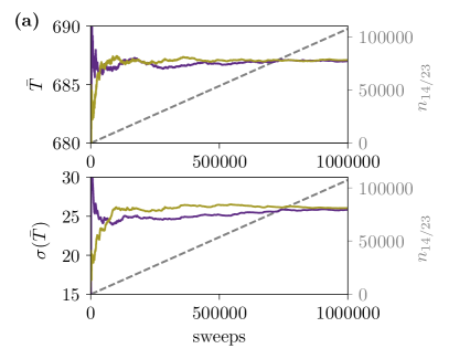
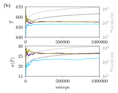
Figure 13: The development of the mean $\bar{T}$ and the standard deviation $\sigma(\bar{T})$ of the travel time values against the number of sweeps. The values for routes 14/23/153 are shown in purple/brown/blue. Part (a) shows measurements of the 4link system for $M=148$ and $n_{\text{l}}^{(j_{1})}=0.5$ and part (b) shows measurements of the 5link system with $L_{5}=278$ and $M=148$ and $n_{\text{l}}^{(j_{1})}\approx 0.92$ and $n_{\text{l}}^{(j_{2})}\approx 0.10$. The second y-axes show how many measurements $n_{14/23/153}$ of $T_{14/23/153}$ were performed. The curve with the long dashes represent the number of measurements of the travel times of route 14 and 23, the curve with the smaller dashes the number of measurements of the travel time of route 153.

A.2 Sweeping the network state - landscapes to find user and system optima

A simple yet CPU time costly way to find the user and system optima is to check all different combinations of $N_{14}$, $N_{23}$ and $N_{153}$, or all combinations $n_{\text{l}}^{(j_{1})}$ and $n_{\text{l}}^{(j_{2})}$, both varying from 0 to 1, for a given $(L_{5},M)$ and see, which combinations minimize $\Delta T$ and $T_{\text{max}}$ respectively. We used a grid resolution of 0.1 for finding the system optima of the 5link system. An example of how the $\Delta T$ and $T_{\text{max}}$ landscapes look like can be seen in Figure 14. It should be noted that the actual system optima may in most cases lie in between the 0.1 grid points. Nevertheless, this grid is sufficient to see whether the system optimum of the 5link system has a lower or higher maximum travel time than that of the 4link system for a given $(L_{5},M)$. It has to be noted though that this technique does not ensure that we found the actual system optima, which is why the coloured points in Figures 12 (a) and (b) should not be seen as accurate values. For finding user optima we used a more accurate method as described in A.3.

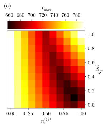
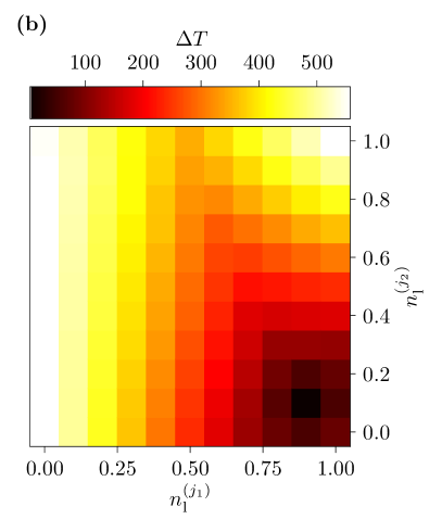
Figure 14: The $\Delta T$ and $T_{\text{max}}$ landscapes of the 5link system for $L_{5}=278$ and $M=148$ depending of the $n_{\text{l}}^{(j_{1})}$ and $n_{\text{l}}^{(j_{2})}$. As can be seen, this is an ”$E_{5}$ optimal” state, since the minima of $\Delta T$ and $T_{\text{max}}$ coincide at $n_{\text{l}}^{(j_{1})}=0.9$ and $n_{\text{l}}^{(j_{2})}=0.1$ and the corresponding strategy has a lower maximum travel time than the 4link’s system optimum which is found at $n_{\text{l}}^{(j_{1})}=0.5$ and $n_{\text{l}}^{(j_{2})}=1.0$.

A.3 Metropolis algorithm for finding user optima

The method of sweeping the $\Delta T$ and $T_{\text{max}}$ landscapes to find user optima, as described in A.2, is not very effective. If the whole region $n_{\text{l}}^{(j_{1})}$ and $n_{\text{l}}^{(j_{2})}$ both from 0 to 1 is sweeped, a lot of measurements are performed far away from the user (and system) optima. Those measurements are a waste of CPU time. Furthermore, depending on how fine the step size is, the user optima will most likely not lie on one of the scanned grid points but in between. A brute force way would be rescanning the corresponding landscape regions with a finer grid. Since this is very time intensive we developed a Metropolis Monte-Carlo [28] algorithm for finding user optima. The algorithm works like this:

1. Set maximum step width $sw$ and ’temperature’ $T$

2. Set start values $(n_{\text{l}}^{(j_{1})},n_{\text{l}}^{(j_{2})})$ and from this

   • $N_{14}=M\cdot n_{\text{l}}^{(j_{1})}\cdot n_{\text{l}}^{(j_{2})}$

   • $N_{23}=M\cdot(1-n_{\text{l}}^{(j_{1})})$

   • $N_{153}=M\cdot n_{\text{l}}^{(j_{1})}\cdot(1-n_{\text{l}}^{(j_{2})})$

3. Let the system thermalize with strategy according to $(n_{\text{l}}^{(j_{1})},n_{\text{l}}^{(j_{2})})$

4. Measure travel times $T_{14}$, $T_{23}$, $T_{153}$ and calculate $\Delta T$

5. Suggest new $(n_{\text{l, new}}^{(j_{1})},n_{\text{l,new}}^{(j_{2})})$ by drawing a random number $z$ between 0 and 2$\pi$ and setting $(n_{\text{l, new}}^{(j_{1})},n_{\text{l, new}}^{(j_{2})})=(n_{\text{l}}^{(j_{1})}+sw\cdot\cos(z),n_{\text{l}}^{(j_{2})}+sw\cdot\sin(z))$ and calculate $N^{\text{new}}_{14}$, $N^{\text{new}}_{23}$, $N^{\text{new}}_{153}$ as in step 2

6. Let the system thermalize with strategy according to $(n_{\text{l, new}}^{(j_{1})},n_{\text{l, new}}^{(j_{2})})$

7. Measure travel times $T^{\text{new}}_{14}$, $T^{\text{new}}_{23}$, $T^{\text{new}}_{153}$ and calculate $\Delta T^{\text{new}}$

8. Accept the new strategy with probability $p=\min\left(1,\exp\left(-\frac{\Delta T-\Delta T^{\text{new}}}{T}\right)\right)$

9. Repeat steps 5 to 7 as long as $\Delta T^{\text{new}}>\epsilon$, with tolerance $\epsilon$

In this algorithm, the maximum step width $sw$ is the maximum possible value, $n_{\text{l}}^{(j_{1})}$ and $n_{\text{l}}^{(j_{2})}$ can be changed by. The temperature $T$ is a measure for the probability with which a strategy with higher $\Delta T$ might be accepted and $\epsilon$ is the tolerance: if $\Delta T\leq\epsilon$ the strategy is accepted as the user optimum. The ’real’ user optimum is reached, if $\epsilon$ is exactly zero. It turned out to be useful to set $\epsilon=20$, $sw=0.1$ and $T=10$. An additional tenth step could be added to the algorithm, in which $sw$ would be reduced, if newly suggested probabilities get rejected a certain amount of times. This additional step was not needed in our case. The algorithm performed well in most of our situations. Fig. 15 (a) shows the search path of the algorithm for $L_{5}=278$ and $M=148$ for 10 different start values $(n_{\text{l}}^{(j_{1})},n_{\text{l}}^{(j_{2})})$. The $uo$-landscape with 0.1 step width as described in the previous subsection is underlayed for visualization purposes.

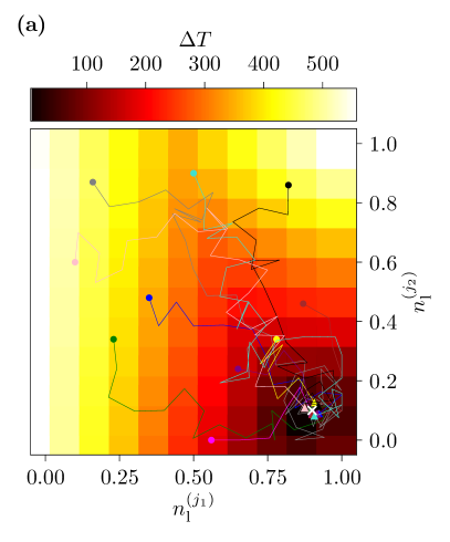
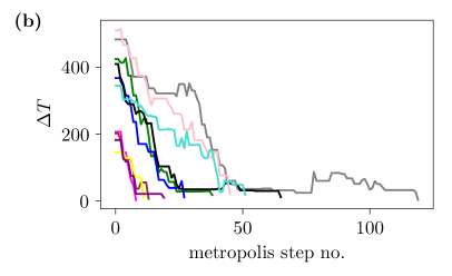
Figure 15: An example of the performance of the Metropolis algorithm for $L_{5}=278$ and $M=148$ and ten different start values. In (a) the search paths are shown with underlayed values of $\Delta T$ which were obtained by sweeping the $(n_{\text{l}}^{(j_{1})},n_{\text{l}}^{(j_{2})})$-landscape as described in A.2. The beginnings of all paths are marked by a $\bigcirc$ and the endings by a $\bigtriangleup$. Also the user optimum is marked by a white $\times$. In (b) the corresponding $\Delta T$ values against the number of Metropolis steps are shown. One can see, that the algorithm converges pretty fast for all 10 start values.

Furthermore, in Fig. 15 (b) the $\Delta T$ values against the Metropolis step nummber (i.e. how often steps 5 to 8 of the algorithm were performed) is shown. From both pictures it can be deduced that the algorithm works really well for this case. Indeed, it performed really well for most other $(L_{5},M)$ combinations as well. Sometimes, depending on the start values, the algorithm will not converge and has to be restarted with different start values. Also in some cases there is more than one user optimum, as described in B. In this case, the algorithm will get ’caught’ in one of them. The algorithm can also be used to find system optima if after each step $T_{\text{max}}$ is calculated and the newly suggested strategy is accepted if $T_{\text{max}}$ got lower. The problem in this case is that there is no real termination condition as there is no a priori known lower bound to $T_{\text{max}}$.

Appendix B Special cases

For some configurations we could find more than one user optimum. Here we present the example of $\hat{L}_{153}/\hat{L}_{14}=0.4$ and $\rho^{(5)}_{\text{global}}=0.18$. In Figure 16 the $T_{\mathrm{max}}$ and $\Delta T$ landscapes for this parameter set are shown. In the figure, the values from a sweep of the landscapes in steps of 0.1 is underlayed.

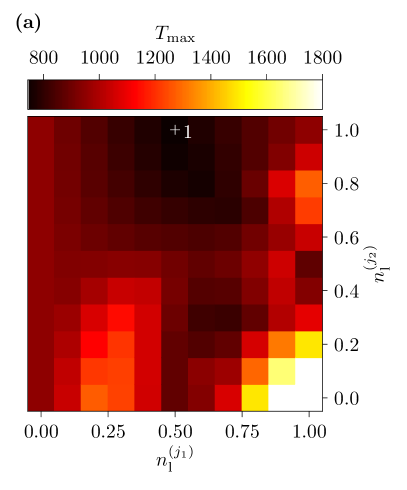
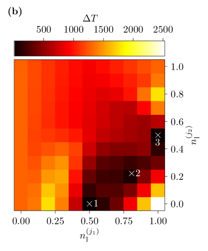
Figure 16: The $T_{\mathrm{max}}$ (part (a)) and $\Delta T$ (part (b)) landscapes of the 5link system with $L_{1}=L_{3}=100$, $L_{2}=L_{4}=500$, $L_{5}=37$, $M=224$, $\rho^{(5)}_{\text{global}}=0.18$. In part (a), the system optimum is marked by $+1$. In part (b) one can see that there are three different user optima, $\times 1$ to $\times 3$, the values of which are given in Table 2.

The travel time and $\Delta T$ and $T_{\mathrm{max}}$ values for the four marked points are given in Table 2. From part (a) of the picture one can see that the system optimum is given by $n_{\text{l}}^{(j_{1})}=0.5$ and $n_{\text{l}}^{(j_{2})}=1.0$. This means that here $so^{(5)}=so^{(4)}$ since this is the state where half of the particles use route 14 and the other half route 23.

In part (b) of the Figure one can see that there are three different user optima. The two user optima $\times 1$ and $\times 3$ were found by sweeping the $n_{\text{l}}^{j_{1}/j_{2}}$ and are special cases of user optima which were already mentioned in Section 2.5. The user optimum $\times 2$ was found by our Metropolis algorithm. The optimum $\times 1$ is a special case since only paths 23 and 153 are used. Since both their travel times are almost equal and smaller than that of the unused route 14 this state is a user optimum. For calculating $\Delta T$, only the difference between $T_{23}$ and $T_{153}$ is used. It would in this case not make sense for any particle to switch to route 14 which has a higher travel time. The same happens in the user optimum $\times 3$, but here routes 14 and 153 are used and route 23 is not. The other user optimum $\times 2$ is an ’ordinary’ user optimum in which all three routes are used and have (almost) the same travel time.

Table 2: The $n_{\text{l}}^{(j_{1}/j_{2})}$, $\Delta T$, $T_{\mathrm{max}}$ and travel time values of the routes for the 4 points which are marked in Figure 16. The points $\times 1$ to $\times 3$ are three user optima of the system, while $+1$ is the system optimum.

Point	$n_{\text{l}}^{(j_{1})}$	$n_{\text{l}}^{(j_{2})}$	$T_{14}$	$T_{23}$	$T_{153}$	$\Delta T$	$T_{\mathrm{max}}$
$\times 1$	0.5	0.0	926	880	876	4	880
$\times 2$	0.808	0.221	970	975	975	10	975
$\times 3$	1.0	0.5	878	1136	875	3	878
$+1$	0.5	1.0	743	742	294	898	743

The (maximum) travel time in all three user optima is higher than that of the system optimum (which is the same as the 4link system optimum) which leads to the conclusion that no matter in which user optimum the system ends up, a ”Braess 1” state is present.

While in the whole unhatched area of the phase diagram (Figure 9) user optima were found we cannot guarantee that all user optima were found. Also, the values (given by the color of the points) in Figures 12 (a) to (c) are given for one of the found user optima and could be slightly different if, for the cases of multiple user optima, another user optimum was chosen. This is because the user optima, as in the example presented here (see Table 2), could have different travel time values. Therefore the values in Figure 12 should not be interpreted as exact values but as a tendency of how the system changes due to the addition of $E_{5}$.

The fact that we found multiple user optima with different travel times (and different $T_{\mathrm{max}}$ values and also different total travel time values) for the same parameter set is also a difference to what is observed in mathematical models of road traffic. In these models it was shown that ”$[$the user optimum$]$ is unique whenever the shortest routes between all pairs of locations are unique and cost is strictly increasing with increasing flow” [29].

References

References

- [1] S. Bittihn, A. Schadschneider, Braess paradox in a network of totally asymmetric exclusion processes, Phys. Rev. E 94 (2016) 062312.
-
[2]
UN population
division, (accessed February 2018).
URL http://www.un.org/en/development/desa/population/ - [3] M. Barthelemy, P. Bordin, H. Berestycki, M. Gribaudi, Self-organization versus top-down planning in the evolution of a city, Scientific Reports 3 (2013) 2153.
- [4] D. Braess, Über ein Paradoxon aus der Verkehrsplanung, Unternehmensforschung 12 (1968) 258.
- [5] D. Braess, A. Nagurney, T. Wakolbinger, On a paradox of traffic planning, Transp. Sc. 39 (2005) 446, (english translation of [4]).
- [6] J. G. Wardrop, Road paper. Some theoretical aspects of road traffic research, Proceedings of the Institution of Civil Engineers 1 (3) (1952) 325–362.
- [7] R. Steinberg, W. Zangwill, The prevalence of Braess’ paradox, Transp. Sci. 17 (1983) 301.
- [8] E. Pas, S. L. Principio, Braess’ paradox: Some new insights, Transportation Research Part B: Methodological 31 (3) (1997) 265–276.
- [9] A. Nagurney, The negation of the Braess paradox as demand increases: The wisdom of crowds in transportation networks, EPL 91 (2010) 48002.
- [10] G. Kolata, What if They Closed 42d Street and Nobody Noticed?, The New York Times, December (1990).
- [11] C. M. Penchina, L. J. Penchina, The Braess paradox in mechanical, traffic, and other networks, Am. J. Phys. 71(5) (2003) 479.
- [12] D. Witthaut, M. Timme, Braess’s paradox in oscillator networks, desynchronization and power outage, New Journal of Physics 14 (8) (2012) 083036.
- [13] L. Crociani, G. Lämmel, Multidestination pedestrian flows in equilibrium: A cellular automaton-based approach, Computer-Aided Civil and Infrastructure Engineering 31 (6) (2016) 432–448.
- [14] K. Bhattacharyya, A thermodynamic parallel of the Braess road-network paradox, arXiv:1703.02213.
- [15] C. T. MacDonald, J. H. Gibbs, A. C. Pipkin, Kinetics of biopolymerization on nucleic acid templates, Biopolymers 6 (1) (1968) 1–25.
- [16] G. Schütz, E. Domany, Phase transitions in an exactly solvable one-dimensional exclusion process, J. Stat. Phys. 72 (1993) 277.
- [17] B. Derrida, M. Evans, V. Hakim, V. Pasquier, Exact solution of a 1d asymmetric exclusion model using a matrix formulation, J. Phys. A 26 (1993) 1493.
- [18] R. Blythe, M. Evans, Nonequilibrium steady states of matrix product form: a solver’s guide, J. Phys. A 40 (2007) R333.
- [19] I. Neri, N. Kern, A. Parmeggiani, Totally asymmetric simple exclusion process on networks, Phys. Rev. Lett. 107 (2011) 068702.
- [20] I. Neri, N. Kern, A. Parmeggiani, Modeling cytoskeletal traffic: An interplay between passive diffusion and active transport, Phys. Rev. Lett. 110 (2013) 098102.
- [21] I. Neri, N. Kern, A. Parmeggiani, Exclusion processes on networks as models for cytoskeletal transport, New Journal of Physics 15 (8) (2013) 085005.
- [22] L. Ming-Zhe, L. Shao-Da, W. Rui-Li, Asymmetric simple exclusion processes with complex lattice geometries: A review of models and phenomena, Chinese Physics B 21 (9) (2012) 090510.
- [23] B. Embley, A. Parmeggiani, N. Kern, Understanding totally asymmetric simple-exclusion-process transport on networks: Generic analysis via effective rates and explicit vertices, Phys. Rev. E 80 (2009) 041128.
- [24] R. Selten, T. Chmura, T. Pitz, S. Kube, M. Schreckenberg, Commuters route choice behaviour, Games and Economic Behavior 58 (2) (2007) 394 – 406.
- [25] A. Rapoport, T. Kugler, S. Dugar, E. J. Gisches, Choice of routes in congested traffic networks: Experimental tests of the braess paradox, Games and Economic Behavior 65 (2) (2009) 538–571.
- [26] T. Thunig, K. Nagel, Braess’s paradox in an agent-based transport model, Procedia Computer Science 83 (2016) 946–951.
- [27] A. C. Pigou, The economics of welfare, Palgrave Macmillan, 2013.
- [28] N. Metropolis, A. W. Rosenbluth, M. N. Rosenbluth, A. H. Teller, E. Teller, Equation of state calculations by fast computing machines, The Journal of Chemical Physics 21 (6) (1953) 1087–1092.
- [29] M. Beckmann, C. B. McGuire, C. B. Winsten, Studies in the economics of transportation, Tech. rep. (1956).