Quantum Entanglement In Inhomogeneous 1D Systems

Abstract

The entanglement entropy of the ground state of a quantum lattice model with local interactions usually satisfies an area law. However, in 1D systems some violations may appear in inhomogeneous systems or in random systems. In our inhomogeneous system, the inhomogeneity parameter, $h$, allows us to tune different regimes where a volumetric violation of the area law appears. We apply the strong disorder renormalization group to describe the maximally entangled state of the system in a strong inhomogeneity regime. Moreover, in a weak inhomogeneity regime, we use a continuum approximation to describe the state as a thermo-field double in a conformal field theory with an effective temperature which is proportional to the inhomogeneity parameter of the system. The latter description also shows that the universal scaling features of this model are captured by a massless Dirac fermion in a curved space-time with constant negative curvature $R=−h^{2}$, providing another example of the relation between quantum entanglement and space-time geometry. The results we discuss here were already published before, but here we present a more didactic exposure of basic concepts of the rainbow system for the students attending the Latin American School of Physics “Marcos Moshinsky” 2017.

1 INTRODUCTION

For bipartite systems, the von Neumann entropy of the reduced density matrix is a measure of the quantum entanglement [1]. The entanglement entropy of the ground state of quantum lattice 1D models satisfies an area law which also provides a link between geometry and quantum structure [2]. For the area law in 1D, the Hastings theorem [3] was proved for local Hamiltonians with finite interaction and a gap in the energy spectrum. Moreover, violations to the area law in 1D may appear in non-local Hamiltonians with divergent interactions or gapless systems. In the latter case, for translational invariant gapless systems which can be described by a conformal field theory (CFT), the area law is restored by a massive perturbation, thus the entanglement entropy is proportional to the logarithm of the correlation length in the scaling regime [4].

In this work we present a much stronger violation of the area law. We deform a 1D critical Hamiltonian with open boundary conditions (OBC) by choosing the exchange couplings from an exponentially-decay function from the centre of the chain. This decrease of the exchange couplings yields to a vanishing gap in the thermodynamic limit [5].

We are able to use just one parameter to describe the inhomogeneity of the system, i.e. the decay rate of the exchange couplings. In terms of that inhomogeneity parameter, $h$, we study two different regimes: the strong disorder regime and the weak disorder regime. An analysis in terms of entanglement entropy and entanglement spectrum was used to discuss the intermediate regime where there is a smooth crossover between the critical system and the maximally entangled ground state without a phase-transition [5].

In the strong disorder regime, i.e. the exchange couplings decay very fast, we use the Dasgupta-Ma Renormalization Group [6], which was also reformulated to study fermionic systems [2], in order to describe the ground state as a valence bond state formed by bonds joining the sites located symmetrically with respect to the centre. This state was also termed as the concentric singlet phase [7] and has a rainbow-like structure illustrated in Figure 1. In the weak inhomogeneity regime, we use a continuum approximation to describe the state as a thermo-field double in a CFT with an effective temperature which is proportional to the inhomogeneity parameter of the system. This latter description also shows that the universal scaling features of this model are captured by a massless Dirac fermion in a curved space-time with constant negative curvature $R=−h^{2}$. Such relation between quantum entanglement and geometry helps explain thermal effects in quantum field theories studied on curved backgrounds, e.g. the Unruh effect where from the point of view of an accelerated observer, the temperature measured in a Minkowski vacuum must be proportional to its acceleration [8].

Experiments using ultracold atomic gases [9] have been used as quantum simulators in order to explore different relations between quantum mechanics and curved space-time, such as the Dirac equation in an artificial curved space-time [10], simulation of $D+1$ dimensions using a $D$-dimensional quantum system based in optical lattices [11], or the dynamics of quantum many-body systems in manifolds with a non-trivial topology like a Möbius strip [12]. Thus, in this work we present how to relate a tunable parameter, i.e. the inhomogeneity in exchange couplings, to a curved space-time which may be also seen as a CFT with an effective temperature.

This work is organised as follows, in a first section we introduce the rainbow model and present the methods used to obtain the entanglement entropy. In a second section we discuss the behaviour of the entanglement entropy as an evidence of the violation of the area law. Furthermore, we analyse the system in both regimes, the strong disorder and the weak disorder, where we present the quantum state obtained in both regimes: a maximally entangled state and a thermal state. After that, we discuss the relation between the inhomogeneous system and a curved space-time. In a final section we present some conclusions and some future works.

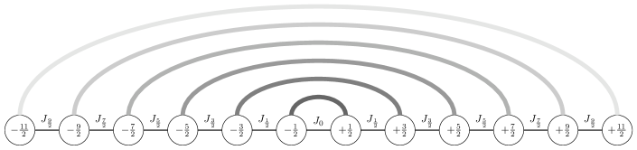
Figure 1: Rainbow model using a system of $2L=12$ sites, which are labeled with half-integers $\pm m/2$ index in order to simplify the notation. Values $\{J_{m}\}$ represent the power-law decreasing exchange couplings between next neighbours. The single bonds connecting the $(-k/2,k/2)$ sites represent Bell pairs established at different scales of energy. Bold grey colour represents a larger scale of energy. A full-colour version of this diagram can be found in [5] where the exchange couplings are given in a logarithmic scale.

2 INHOMOGENEOUS 1D SYSTEMS

We are interested in inhomogeneous systems because, as we will show, they can present a strong violation of the area law. The inhomogeneity of the exchange couplings in many-body systems has been addressed from different points of view, e.g. smooth changes can be regarded as position-dependent speed of propagation for the excitation, such as a local gravitational potential [10] or a horizon [5]. Moreover, an exponential dependence of the exchange couplings with the position is a characteristic of Kondo-like problems [13] and systems with an hyperbolic dependence of the couplings with the position has been used to study the scaling properties of non-deformed systems [14, 15]. However, smoothed boundary conditions, i.e. the couplings fall to zero near the borders, have been used to reduce the finite-size effects when measuring bulk properties of the ground state [16].

2.1 The Rainbow Model

Consider a fermionic system with $2L$ sites which are labeled with half-integers $\pm m/2$, in order to simplify the notation. As usual, positive numbers are used for sites placed from the centre of the system to its right border, cf. Figure 1. For OBC, the dynamics of the system is given by the Hamiltonian

$$H=-\frac{J_{0}}{2}c^{\dagger}_{\frac{1}{2}}c_{-\frac{1}{2}}-\sum_{m=\frac{1}{2}}^{L-\frac{3}{2}}\frac{J_{m}}{2}\left[c^{\dagger}_{m}c_{m+1}+c^{\dagger}_{-m}c_{-m-1}\right]+h.c.$$ (1)

where $J_{0}$ sets the scale for the exchange couplings, $c_{m}$ and $c^{\dagger}_{m}$ denote the annihilation and creation operators of a spinless fermion at the site $m$. The values $\{J_{m}\}$ follow an exponentially-decay function from the centre of the chain

$$J_{m}=J_{0}e^{-hm},$$

$h\geq 0$ characterises the inhomogeneity of the exchange couplings, i.e. it determines the inhomogeneity of the system. The case $h=0$ corresponds to the standard uniform Hamiltonian of a spinless free fermion with OBC [5, 2] and its low energy properties are captured by a CFT with central charge $c=1$, i.e. the massless Dirac fermion theory, or equivalently a Luttinger liquid with Luttinger parameter $K=1$ [17].

It has been shown that other decay functions also results in concentric singlet phases [7]. Moreover, only an exponentially-decay function allows us to move smoothly from the homogeneous case, $h=0$, to a maximally entangled state.

2.2 Entanglement Over The Rainbow

In case the exchange couplings have very different values, we can apply the strong disorder renormalization group (SDRG) method [6] which was reformulated to include the fermionic nature of the particles [2]. The RG method starts by picking up the strongest coupling and then to establish a singlet bond (a valence bond state) on top of it and then using an effective coupling, which is obtained using second order perturbation theory, between the two neighbours of the singlet

$$\tilde{J}=-\frac{J_{L}J_{R}}{J_{max}},$$ (2)

where $J_{L}$ and $J_{R}$ are, respectively, the left and right couplings to the maximal one, $J_{max}$, which establish the scale of energy where the RG step is done. A detailed procedure to obtain the relation in (2) for spins was presented by Casa Grande et al. [18] and the arguments to extend the method to fermionic particles was presented by Ramirez et al. [2]. See in Figure 1, the different scales of energy are represented by the grey scale, a bold colour represents more energy.

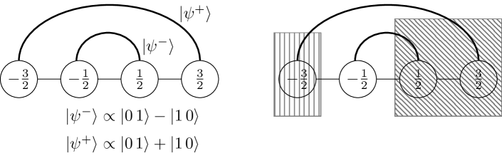
Figure 2: Left panel: Bell pair states localised at different RG steps. In a first RG step, the singlet-type state, $|\psi^{-}\rangle$, is established with a bond connecting lattice sites $(-1/2,1/2)$. In a second RG step the triplet-type state, $|\psi^{+}\rangle$, is established with a bond connecting lattice sites $(-3/2,3/2)$. The sign change from negative to positive relates the fermion nature of the particles. Right panel: Examples of the blocks of lattice sites which can be obtained in different bipartitions of the system. The block with the vertical-line pattern contains only one site, it represents the system’s bipartition $[-3/2]\cup[-1/2,1/2,3/2]$, and its block-entropy is proportional to the number of bonds connecting the block with the rest of the system. The block with the diagonal-line pattern contains two sites representing other bipartition, each site with a bond connecting the rest of the system.

The renormalization step represents to localise a Bell pair state, or a bond, between sites connected by $J_{max}$, cf. left panel Figure 2. Moreover, equation (2) implies that the effective couplings can be either positive or negative in relation to the nature of the established bond [2], thus there are singlet-type bonds $|\psi^{-}\rangle\propto|01\rangle-|10\rangle$ and triplet-type bonds $|\psi^{+}\rangle\propto|01\rangle+|10\rangle$. Both types of bonds share many properties such as the entanglement [2]. The procedure is repeated until the $2L$ sites are linked by $L$ bonds establishing a valence bond structure. See left panel in Figure 2 for a graphical example of two bonds established in successive RG steps. The first bond establishes a singlet-type bond $|\psi^{-}\rangle$ connecting sites $(-1/2,1/2)$ at an energy-scale given by $J_{0}$. The distribution of values of $J_{m}$ is such that the second RG step establishes a bond connecting sites $(-3/2,3/2)$, however this is a triplet-type bond.

Once the valence bond structure is completed, the von Neumann entropy for a block $B$ can be easily computed with

$$S(B)=n_{B}\log{(2)},$$ (3)

where $n_{B}$ is the number of bonds joining $B$ with the rest of the system, i.e. the number of broken Bell pairs. See right panel in Figure 2 for a graphical example of two blocks which may be obtained in different system’s bipartitions. The block with the vertical-line pattern is obtained with the system’s bipartition $[-3/2]\cup[-1/2,1/2,3/2]$ thus, the block is formed by only one site, i.e. its size is one, which is connected to the rest of the system by one bond. The block with diagonal-line pattern is obtained splitting the system in half, here there are two sites each one with a bond connecting the block with the rest of the system. The computation of the von Neumann entropy becomes a process of counting the bonds connecting the block of interest. Nevertheless, in the RG approximation, all the Rényi entropies take the same value of the von Neumann entropy [5].

Since the Hamiltonian (1) is quadratic in the fermionic operators, the exact diagonalization method [5] can be used to obtain the properties of the system using a canonical transformation for the fermionic operators $c^{\dagger}$ and $c$, such that

$$\bar{\psi}^{k}=\sum_{i}v_{k,i}c_{i}^{\dagger},$$

are the single-body modes, with single-body energy $\epsilon_{k}$ associated, for which the Hamiltonian (1) is diagonal, $v_{k,i}$ is a unitary matrix obtained by the diagonalization of the hopping matrix. Thus, the ground state of the system is obtained by filling $L$ fermions in the set $\Omega$ of single-body modes with energy below the Fermi level, i.e. $\Omega=\{k|\epsilon_{k}<\epsilon_{F}\}$. These occupied single-body modes, $\psi^{k}$, can be used to compute the correlation matrix [5, 2]

$$C_{ij}=\langle GS|c^{\dagger}_{i}c_{j}|GS\rangle=\sum_{k\in\Omega}\bar{\psi}^{k}_{i}\psi^{k}_{j},$$

where $i$ and $j$ label sites which are both inside the considered block $B$. The eigenvalues $\{\nu_{p}\}$ of the correlation matrix determine the $n$-order Rényi entropies for the block $B$ of the system, so

$$S^{(n)}(B)=\frac{1}{1-n}\sum_{p}\log{[\nu_{p}^{n}+(1-\nu_{p})^{n}]},$$

and the von Neumann entropy can be obtained from the limit $n\to 1$. The scaling behaviour of the entanglement entropy of a block $B$ of size $\ell$ is known to be

$$\begin{split}S^{(n)}(\ell)\simeq&\frac{c}{12}\left(1+\frac{1}{n}\right)\log{\left[\frac{4L}{\pi}\sin{\left(\frac{\pi\ell}{2L}\right)}\right]}+c^{\prime}_{n}\\ &+f_{n}\cos{(\pi\ell)}\left[\frac{8L}{\pi}\sin{\left(\frac{\pi\ell}{2L}\right)}\right]^{-K/n},\end{split}$$ (4)

where the first term is given by the CFT associated for homogeneous free fermion model, $c^{\prime}_{n}$ is a non-universal constant, the last term accounts for the fluctuations at Fermi momentum, $k_{F}=\pi/2$, and the constants $f_{n}$ can be obtained analytically [19]

$$f_{n}=\frac{2}{1-n}\left[\frac{\Gamma\left(\frac{1}{2}+\frac{1}{2n}\right)}{\Gamma\left(\frac{1}{2}-\frac{1}{2n}\right)}\right],$$

where $f_{1}\equiv 1$ by definition.

3 RESULTS

Using the methods described above, we are able to obtain the entanglement properties of the system. Selecting the inhomogeneity parameter, $h$, we are able to set the system in two regimes: The strong disorder and the weak disorder regime. The RG method explains with simple terms the violation to the area law, but it describes all the Rényi entropies to be the same as the von Neumann entanglement entropy. Nevertheless, the exact diagonalization method is applicable to all values of $h$. It was showed that the system moves in the two regimes without phase transitions [5].

To give a full description of the rainbow model first we show that the violation of the area law appear for $h\geq 0$. Although for $h=0$, the logarithmic violation is well described by CFT, there appears a volumetric behaviour in the entanglement entropy for $h>0$. Thus, we apply the RG method for $h\gg 0$, i.e. the strong disorder regime, to describe the structure of the ground state in terms of the valence bond structure obtained in each RG’s step. Furthermore, we use an analytic continuation in the limit $h\ll 1$, i.e. the weak disorder regime, to describe the ground state as a thermal state. Moreover, we show that this state is related to the one described by a massless Dirac fermion theory in a curved space-time, thus this analysis could help to explain thermal effects in quantum field theories studied on curved backgrounds.

3.1 Violation of the Area Law

As stated above, the area law is violated for all the values of the inhomogeneity parameter. The logarithmic violation appear in the limit $h=0$, i.e. the uniform system, it corresponds to a spinless free fermion system, its low energy properties are described by a CFT with $c=1$. The entanglement entropy for a block of size $\ell$ is given in equation (4). However, we focus in blocks of one half of the system in order to simplify the analysis of the functional dependence of the entropy, thus, the entanglement entropy is [5]

$$S_{CFT}(L)=\frac{c}{6}\log{(L)}+c^{\prime}+f_{1}\frac{\cos{(\pi L)}}{L^{K}},$$ (5)

where $c^{\prime}$ is an additive constant which includes the boundary entropy and non-universal contributions [4, 20], $f_{1}$ is a measure of the amplitude of the oscillations, which were shown to vanish as the inhomogeneity of the system increases [5]. The left panel in Figure 3 shows a fit of the half chain entanglement entropy, Equation (5), for different values of the system half chain $L$. This logarithmic behaviour represents a violation of the area law with a leading term proportional to $\log{(L)}$.

Figure 3: Left: Entanglement entropy for one half of the chain $S_{CFT}(L)$ as a function of the half size of the system $L$ for the uniform system. The line corresponds to the fit given to Equation (5). Right: Entanglement entropy for the inhomogeneous system as a function of the half size of the system for different values of $z\equiv hL$.

The volumetric violation of the area law appear for all values $h>0$. It is convenient to define an effective size of the system $z\equiv hL$ for the given inhomogeneity in the system in order to simplify the functional analysis and the notation. In terms of this effective size of the system, the strong disorder regime appear for $z\gg 1$ and the weak disorder regime appear for $z\ll 1$. This change in the effective size of the system anticipates some relation between the inhomogeneity of the system and its geometry.

The right panel in Figure 3 shows the entanglement entropy of the half of the chain as a function of the system size for $z=5$ and for $z=9$, i.e. both $L$ and $h$ varies in order to keep $z$ constant. The entanglement entropy shows a linear behaviour which was explained as [5]

$$S(L)=\frac{c(z)}{6}\log{(L)}+d(z)+f(z)\frac{\cos{(\pi L)}}{L^{K}},$$ (6)

where $c(z)$, $d(z)$ and $f(z)$ are now functions of $z$ and explain the behaviour of the entanglement entropy for different values of the inhomogeneity. For the limit $z\gg 1$, functions $c(z)\to 0$, $d(z)\to 0.318z$ and $f(z)\to 0$ [5] thus, the entanglement entropy is expected to have a linear behaviour $S(L)\to 0.318\,hL$, but in the strong inhomogeneity limit it should behave as $S(L)=L\log{(2)}$ as discussed above.

Table 1: Summary of the different Area law’s violation for all the regimes of the Rainbow Model

		Violation	Leading
Regime	Description	type	term
$h=0$ (uniform)	CFT	logarithmic	$\propto\log{(L)}$
$h\ll 1$ (weak disorder)	thermal-state	volumetric	$\propto L$
$h\gg 1$ (strong disorder)	valence bond states	volumetric	$\propto L$

In Table 1 we present a summary of the violations of the area law for the different regimes of the rainbow model. Note that the area law is violated in all cases by the model. The model can be reduced to its homogeneous, or uniform, case for $h=0$ where the CFT associated characterises a ground state which violates the area law with a logarithmic dependence of the size of the system. The cases of weak disorder and strong disorder have a ground state which violates the area law with a volumetric behaviour because the function $d(z)$, cf. Equation (6), becomes the leading term as the inhomogeneity of the system grows. It should be noticed that the function $c(z)$ decreases monotonously as the inhomogeneity of the system grows in agreement to the Zamolodchikov c-theorem [5].

3.2 Strong Disorder Regime

This regime is well explained by the SDRG described above. At the beginning of the RG method, the central link is used to renormalize the two central sites, it establishes the scale of energy. The effective link, obtained with the Equation (2), sets the new scale of energy, and the procedure is repeated. When the RG procedure is done, the GS can be obtained as the product of valence bond states connecting the $(-k/2,k/2)$ sites. Nevertheless, in terms of the bonding and anti-bonding operators defined as [2]

$$(b^{+}_{ij})^{\dagger} = \frac{1}{\sqrt{2}}\left(c^{\dagger}_{i}+c^{\dagger}_{j}\right),$$

$$(b^{-}_{ij})^{\dagger} = \frac{1}{\sqrt{2}}\left(c^{\dagger}_{i}-c^{\dagger}_{j}\right),$$

the GS of the Hamiltonian (1) is given by

$$|R(L)\rangle\equiv\left(b^{S_{L}}_{-L+\frac{1}{2},L-\frac{1}{2}}\right)^{\dagger}\cdots\left(b^{+}_{-\frac{5}{2},\frac{5}{2}}\right)^{\dagger}\left(b^{-}_{-\frac{3}{2},\frac{3}{2}}\right)^{\dagger}\left(b^{+}_{-\frac{1}{2},\frac{1}{2}}\right)^{\dagger}|0\rangle,$$ (7)

where $S_{L}=(-1)^{L}$. The entanglement entropy for a block is obtained by counting the number of links connecting the block with the rest of the system, cf. Figure 2. For a block of the half of the system, $n_{B}=L$ thus, we obtain a maximally entangled state and it fulfills a volume law. The energy gap can be estimated as the effective energy of the last bond established, i.e. $\alpha^{2L}$ in Figure 1. Thus the gap vanishes in the limit $L\to\infty$ in agreement with the Hastings theorem [5].

3.3 Weak Disorder Regime

In this regime, a continuum approximation of the Hamiltonian (1) is obtained by expanding the local operator $c_{n}$ into the slow chiral modes, $\psi_{R}(x)$ and $\psi_{L}(x)$ around the Fermi points $\pm k_{F}$

$$\frac{c_{n}}{\sqrt{a}}\simeq e^{ik_{F}x}\psi_{L}(x)+e^{-ik_{F}x}\psi_{R}(x),$$ (8)

and located at the position $x=an\in(-{\cal L,L})$, where $a={\cal L}/L$ is the lattice spacing. Using Equation (8) in (1) we obtain

$$H\simeq\frac{ia}{2}\int_{-\cal L}^{\cal L}dx\;e^{-\frac{h|x|}{a}}\left[\psi^{\dagger}_{R}\partial_{x}\psi_{R}-(\partial_{x}\psi^{\dagger}_{R})\psi_{R}-\psi^{\dagger}_{L}\partial_{x}\psi_{L}+(\partial_{x}\psi^{\dagger}_{L})\psi_{L}\right],$$ (9)

assuming that the fields $\psi_{R,L}(x)$ vary slowly with $x$ in order to drop some cross terms. This Hamiltonian (9) describes the low energy excitations of the original lattice Hamiltonian and can also be brought to the standard canonical form of a free fermion with OBC [2]. A change in the variables

$$\tilde{x}=\mathrm{sign}(x)\frac{e^{h|x|}-1}{h},$$ (10)

in terms of the inhomogeneity of the system $h$, maps the interval $x\in[-L,L]$ into the interval $\tilde{x}\in[-\tilde{L},\tilde{L}]$. The transformation for the fermion fields are

$$\tilde{\psi}_{R,L}(\tilde{x})=\left(\frac{d\tilde{x}}{dx}\right)^{-1/2}\psi_{R,L}(x),$$

which can be used to transform the Hamiltonian (9) to

$$H\simeq i\int_{-\tilde{L}}^{\tilde{L}}d\tilde{x}\left[\tilde{\psi}_{R}^{\dagger}\partial_{\tilde{x}}\tilde{\psi}_{R}-\tilde{\psi}_{L}^{\dagger}\partial_{\tilde{x}}\tilde{\psi}_{L}\right],$$

which is the free fermion Hamiltonian for a chain of size $2\tilde{L}$. A prediction of the entanglement entropy for the deformed chain is given by [2]

$$S(L)=\frac{c}{6}\log{\left(\frac{e^{hL}-1}{h}\right)}+c^{\prime}=\frac{c}{6}\log{(\tilde{L})}+c^{\prime},$$

for larger systems, which can be compared with the equation given by the CFT in Equation (5) by means of the transformation of variables given in Equation (10). This relation allowed the comparison of the entanglement entropy in the limit $h\to 0^{+}$ with the entropy of a thermal state at temperature $T=1/\beta$ in a CFT [4] in order to relate

$$T=\frac{1}{\beta}=\frac{h}{2\pi},$$ (11)

thus, the rainbow state is similar to a thermal state with an effective temperature proportional to the inhomogeneity of the system, $h$.

Recently, the relation between quantum entanglement and the geometry of the space-time where the system lives motivates the study of links between geometry and quantum structure given the area-laws. It was shown that the rainbow Hamiltonian can be obtained from the action of a massless Dirac fermion in a curved space-time [17].

The interest in models with smoothly varying couplings and quantum field theories in curved space-times has been put forward in [10, 21], with potential cold atom realisations in sight. In addition to those proposals for tabletop experiments that mimic effects from high-energy physics, there is another good reason for exploring the relevance of quantum field theory in curved space for the physics of ultracold quantum gases. Most experimental setups involve trapping potentials, often harmonic ones, that result in inhomogeneous density profiles in the models one wants to simulate; in fact, the presence of non-uniform potential wells, or background electromagnetic fields, is the rule rather than the exception. It was pointed out very recently [22], in the study of non-interacting fermion gases in $1+1$ dimensions, that the inhomogeneity generated by the trapping potential are captured by quantum field theory in curved space-time.

This derivation is done using the covariant formalism of relativistic field theory with Minkowski signature. The Lagrangian associated to the Hamiltonian (1) is

$$\begin{split}{\cal L}=&\psi_{-}^{\dagger}\partial_{0}\psi_{-}+\psi_{+}^{\dagger}\partial_{0}\psi_{+}+e^{-h|x^{1}|}\left(\psi_{-}^{\dagger}\partial_{1}\psi_{-}-\psi_{+}^{\dagger}\partial_{1}\psi_{+}\right)\\ &+\frac{h}{2}\mathrm{sign}(x^{1})e^{-h|x^{1}|}(\psi_{+}^{\dagger}\psi_{+}-\psi_{-}^{\dagger}\psi_{-}),\end{split}$$ (12)

where $\psi_{-}=\psi_{L}$, $\psi_{+}=\psi_{R}$, and the coordinates are $(t,x)=(x^{0},x^{1})$ and $\partial_{\mu}=\partial/\partial x^{\mu}$. For $h=0$ the Equation (12) becomes the Dirac action of a massless fermion in $1+1$ dimensions. The flat space-time metric, denoted by $\eta^{ab}(a,b=0,1)$, has the signature $(-,+)$. In order to express the Lagrangian (12) as the Dirac action in curved space-time we need the metric $g_{\mu\nu}$, the zweibein $e^{a}_{\mu}$, its inverse $E^{\mu}_{a}$, the spin connection $\omega_{\mu}^{ab}$ and the Christoffel symbols $\Gamma^{\nu}_{\lambda\mu}$ which are related as

$$g_{\mu\nu} = \eta_{ab}e^{a}_{\mu}e^{b}_{\nu},$$

$$E^{\mu}_{a} = g^{\mu\nu}\eta_{ab}e^{b}_{\nu},$$

$$\omega_{\mu}^{ab} = e^{a}_{\nu}\partial_{\mu}E^{b\nu}+e^{a}_{\nu}E^{b\lambda}\Gamma^{\nu}_{\lambda\mu},$$

now, the Dirac Lagrangian of a massless fermion in curved space-time is

$${\cal L}=e\bar{\psi}{\not{D}}\psi,$$

where ${\not{D}}=E^{\mu}_{a}\gamma^{a}D_{\mu}$ and $e=\mathrm{det}e^{a}_{\mu}$, thus comparing equations and solving for the space-time metric, we obtain $g_{00}=-e^{-2h|x|}$ and $g_{11}=1$ and with the non-vanishing components of the Christoffel symbols and the Ricci tensor yield the scalar curvature

$$R(x)=g^{\mu\nu}R_{\mu\nu}(x)=4h\delta(x)-h^{2},$$

that is constant and negative here except at the origin where it is singular [17].

4 CONCLUSIONS

In this work we presented how to parametrise the inhomogeneity of a 1D system whose dynamics is described by the local Hamiltonian (1). The variation of the inhomogeneity parameter, $h$, allowed us to move the system between two different violations of the area law without a phase transition.

In the strong disorder regime the behaviour of the entanglement entropy is explained with the structure of the ground state (7). The entanglement entropy for this state is obtained as described by Equation (3), counting the number of links connecting the block of interest with the rest of the system. It represents a linear growth of the entanglement entropy with the size of the system. But, since the gap of the system vanishes in the limit $L\to\infty$ the Hastings theorem is kept.

In the weak inhomogeneity limit, a continuum approximation can be found to relate the system to a homogeneous one. The rainbow system can be viewed as a conformal system at a finite temperature proportional to the inhomogeneity of the system as can be seen in Equation (11). The universal scaling features of the rainbow model are captured by a massless Dirac fermion in a curved space-time with constant negative curvature.

5 ACKNOWLEDGEMENTS

We would like to acknowledge G Sierra and J Rodríguez-Laguna for their useful comments and support. We also acknowledge financial support from the Dirección General de Docencia at the Universidad de San Carlos de Guatemala and from the Organizing Committee of the Latin American School of Physics “Marcos Moshinsky” 2017.

References

- [1] Luigi Amico, Rosario Fazio, Andreas Osterloh, and Vlatko Vedral. Entanglement in many-body systems. Rev. Mod. Phys., 80:517–576, 2008.
- [2] G. Ramírez, J. Rodríguez-Laguna, and G. Sierra. Entanglement over the rainbow. J. Stat. Mech., 2015(6):P06002, 2015.
- [3] M. B. Hastings. An area law for one-dimensional quantum systems. J. Stat. Mech., 2007(08):P08024, 2007.
- [4] Pasquale Calabrese and John Cardy. Entanglement entropy and quantum field theory. J. Stat. Mech., 2004(06):P06002, 2004.
- [5] G. Ramírez, J. Rodríguez-Laguna, and G. Sierra. From conformal to volume law for the entanglement entropy in exponentially deformed critical spin 1/2 chains. J. Stat. Mech., 2014(10):P10004, 2014.
- [6] Chandan Dasgupta and Shang-keng Ma. Low-temperature properties of the random Heisenberg antiferromagnetic chain. Phys. Rev. B, 22(3):1305–1319, 1980.
- [7] G. Vitagliano, A. Riera, and J. I. Latorre. Volume-law scaling for the entanglement entropy in spin-1/2 chains. New J. Phys., 12(11):113049, 2010.
- [8] Sandra Robles and Javier Rodríguez-Laguna. Local quantum thermometry using unruh–dewitt detectors. J. Stat. Mech., 2017(3):033105, 2017.
- [9] M. Lewenstein, A. Sanpera, and V. Ahufinger. Ultracold Atoms in Optical Lattices: Simulating quantum many-body systems. OUP Oxford, 2012.
- [10] O. Boada, A. Celi, J. I. Latorre, and M. Lewenstein. Dirac equation for cold atoms in artificial curved spacetimes. New J. Phys., 13(3):035002, 2011.
- [11] O. Boada, A. Celi, J. I. Latorre, and M. Lewenstein. Quantum simulation of an extra dimension. Phys. Rev. Lett., 108:133001, Mar 2012.
- [12] Octavi Boada, Alessio Celi, Javier Rodríguez-Laguna, José I Latorre, and Maciej Lewenstein. Quantum simulation of non-trivial topology. New J. Phys., 17(4):045007, 2015.
- [13] Kouichi Okunishi and Tomotoshi Nishino. Scale-free property and edge state of Wilson’s numerical renormalization group. Phys. Rev. B, 82:144409, 2010.
- [14] Hiroshi Ueda and Tomotoshi Nishino. Hyperbolic Deformation on Quantum Lattice Hamiltonians. J. Phys. Soc. Jpn., 78(1):014001, 2009.
- [15] Hiroshi Ueda, Hiroki Nakano, Koichi Kusakabe, and Tomotoshi Nishino. Scaling Relation for Excitation Energy under Hyperbolic Deformation. Prog. Theor. Phys., 124(3):389–398, 2010.
- [16] M. Vekić and S. R. White. Smooth boundary conditions for quantum lattice systems. Phys. Rev. Lett., 71:4283–4286, 1993.
- [17] J. Rodríguez-Laguna, J. Dubail, G. Ramírez, P. Calabrese, and G. Sierra. More on the rainbow chain: entanglement, space-time geometry and thermal states. J. Phys. A: Math. Theor., 50(16):164001, 2017.
- [18] H. L. Casa Grande, N. Laflorencie, F. Alet, and A. P. Vieira. Analytical and numerical studies of disordered spin-1 heisenberg chains with aperiodic couplings. Phys. Rev. B, 89:134408, Apr 2014.
- [19] Maurizio Fagotti and Pasquale Calabrese. Universal parity effects in the entanglement entropy of XX chains with open boundary conditions. J. Stat. Mech., 2011(01):P01017, 2011.
- [20] G. Vidal, J. I. Latorre, E. Rico, and A. Kitaev. Entanglement in quantum critical phenomena. Phys. Rev. Lett., 90:227902, 2003.
- [21] Javier Rodríguez-Laguna, Leticia Tarruell, Maciej Lewenstein, and Alessio Celi. Synthetic unruh effect in cold atoms. Phys. Rev. A, 95:013627, Jan 2017.
- [22] Jérôme Dubail, Jean-Marie Stéphan, Jacopo Viti, and Pasquale Calabrese. Conformal Field Theory for Inhomogeneous One-dimensional Quantum Systems: the Example of Non-Interacting Fermi Gases. SciPost Phys., 2:002, 2017.