IPPP/18/20

Higher-order condensate corrections to $\Upsilon$ masses, leptonic decay rates and sum rules

T. Rauh
IPPP, Department of Physics, University of Durham,
DH1 3LE, United Kingdom

Abstract
With the recent completion of NNNLO results, the perturbative description of the $\Upsilon$ system has reached a very high level of sophistication. We consider the non-perturbative corrections as an expansion in terms of local condensates, following the approach pioneered by Voloshin and Leutwyler. The leading order corrections up to dimension eight and the potential NLO corrections at dimension four are computed and given in analytical form. We then study the convergence of the expansion for the masses, the leptonic decay rates and the non-relativistic moments of the $\Upsilon$ system. We demonstrate that the condensate corrections to the $\Upsilon(1S)$ mass exhibit a region with good convergence, which allows us to extract $\overline{m}_{b}(\overline{m}_{b})=4214\pm 37\,(\text{pert.})\,_{-22}^{+20}\,(\text{non-pert.})\text{ MeV}$, and show that non-perturbative contributions to the moments with $n\approx 10$ are negligible.

1 Introduction

In recent years, the accuracy of the perturbative description of the bottomonium system has been extended to next-to-next-to-next-to-leading order (NNNLO). The full spectrum [2, 1], the leptonic decay rate of the $\Upsilon(1S)$ [4] and the non-relativistic moments of the total $e^{+}e^{-}\to b\bar{b}X$ cross section [5] have been determined and perturbation theory is well behaved. This has important phenomenological implications. For instance, some of the most precise determinations of the bottom-quark mass rely on the comparison of the perturbative expressions for the non-relativistic moments [5, 6, 7, 8] or the masses of the $\Upsilon(1S)$ and $\eta_{b}(1S)$ resonances [9, 10, 11] and recently also the $n=2$ states [12] with their experimental values.

Bottomonium can be treated as a non-relativistic system where the bottom-quark velocity $v$ is of the order of the strong-coupling constant: $v\sim\alpha_{s}(m_{b}v)\ll 1$. There is a large hierarchy between the dynamical scales $m_{b}$ (hard), $m_{b}v$ (soft) and $m_{b}v^{2}$ (ultrasoft) of the system. The perturbative calculations [2, 1, 3, 4, 5] were performed using the effective theory potential non-relativistic QCD (PNRQCD) [13, 14, 15, 16], where the hard and the soft scale have been integrated out and the only dynamical modes left are potential bottom quarks $\psi$ and anti-bottom quarks $\chi$, with energy and momentum of the order $m_{b}v^{2}$ and $m_{b}v$, respectively, as well as ultrasoft gluons and light quarks. The Lagrangian for perturbative calculations up to NNNLO takes the form

$$\mathcal{L}_{\text{PNRQCD}}= \hskip 4.26773pt\psi^{\dagger}\left(i\partial_{0}+\frac{\bm{\partial}^{2}}{2m}+g_{s}A_{0}(t,\mathbf{0})-g_{s}\mathbf{x}\cdot\mathbf{E}(t,\mathbf{0})+\frac{\bm{\partial}^{4}}{8m^{3}}\right)\psi$$ (1)

$$+\chi^{\dagger}\left(i\partial_{0}-\frac{\bm{\partial}^{2}}{2m}+g_{s}A_{0}(t,\mathbf{0})-g_{s}\mathbf{x}\cdot\mathbf{E}(t,\mathbf{0})-\frac{\bm{\partial}^{4}}{8m^{3}}\right)\chi$$

$$+\int d^{d-1}\mathbf{r}\left[\psi_{a}^{\dagger}\psi_{b}\right](x+\mathbf{r})V_{ab;cd}(\mathbf{r},\partial)\left[\chi_{c}^{\dagger}\chi_{d}\right](x)$$

$$+\mathcal{L}_{\text{ultrasoft}},$$

where the coupling to the ultrasoft gluon field in the bottom-quark bilinear parts has been multipole expanded in the spatial components [17], the third line describes the interactions through spatially non-local potentials, which are given in [16, 18], and the ultrasoft Lagrangian is a copy of the QCD Lagrangian which only contains the ultrasoft gluon and light quark fields.

Purely perturbative calculations within PNRQCD are valid when the ultrasoft scale $m_{b}v^{2}$ is much larger than the QCD scale $\Lambda_{\text{QCD}}$. This is certainly the case for top quarks, which are studied in [19, 20], but is questionable in the bottomonium sector. Assuming the hierarchy holds, non-perturbative corrections can be incorporated in terms of local vacuum condensates as a power series in $(\Lambda_{\text{QCD}}/(m_{b}v^{2}))^{2}$, following the approach of Voloshin and Leutwyler [23, 24, 25, 26]. In this work, we compute higher-order corrections in this approach and assess the convergence of the series.

In the limit $\Lambda_{\text{QCD}}\ll m_{b}v^{2}$, the gluon field in the PNRQCD Lagrangian can be split into two parts

$$A_{\mu}(t,\mathbf{x})=A_{\mu}^{\text{us}}(t,\mathbf{x})+A_{\mu}^{\text{np}}(t,\mathbf{x}).$$ (2)

The superscripts denote the ultrasoft and the non-perturbative gluon field with momentum of the order $m_{b}v^{2}$ and $\Lambda_{\text{QCD}}$, respectively. All couplings of the non-perturbative component to other modes must be multipole-expanded because the non-perturbative field with a large wavelength of the order $1/\Lambda_{\text{QCD}}$ cannot resolve the dynamics of the potential bottom quarks or of the ultrasoft gluons. A convenient gauge choice for the non-perturbative gluon field is given by Fock-Schwinger gauge

$$\mathbf{x}\cdot\mathbf{A}^{\text{np}}(t,\mathbf{x})=0,\hskip 28.45274ptA_{0}^{\text{np}}(t,\mathbf{0})=0,$$ (3)

which removes the coupling of the bottom quarks to the $A_{0}^{\text{np}}$ field. The leading non-perturbative contribution in the PNRQCD Lagrangian then takes the form of a chromoelectric dipole term

$$\mathcal{L}_{\text{non-perturbative}}=\psi^{\dagger}\left(-g_{s}\mathbf{x}\cdot\mathbf{E}^{\text{np}}(0,\mathbf{0})+\dots\right)\psi+\chi^{\dagger}\left(-g_{s}\mathbf{x}\cdot\mathbf{E}^{\text{np}}(0,\mathbf{0})+\dots\right)\chi,$$ (4)

and is of the order $m_{b}^{2}v^{2}\Lambda_{\text{QCD}}^{2}$ because $\mathbf{E}^{\text{np}}\sim\Lambda_{\text{QCD}}^{2}$ and the strong coupling at the QCD scale is counted as order one. This implies that the chromoelectric dipole coupling to the non-perturbative gluon field is suppressed by $v(\Lambda_{\text{QCD}}/(m_{b}v^{2}))^{2}$ with respect to the leading order Lagrangian. The time-dependent terms in the multipole expansion and the expanded couplings between the non-perturbative and ultrasoft modes in $\mathcal{L}_{\text{ultrasoft}}$ are not required for the leading order condensate corrections. Their relevance at higher orders is assessed in Section 3, where we discuss the NLO QCD corrections to the leading term in the Voloshin-Leutwyler approach.

The condensate corrections to the considered observables can be extracted from the non-relativistic Green function at the origin

$$G(E)\equiv\bm{\langle}\bm{\langle}\mathbf{0}\bm{|}\bm{|}\left(\hat{H}-E-i0\right)^{-1}\bm{|}\bm{|}\mathbf{0}\bm{\rangle}\bm{\rangle},$$ (5)

where $E=\sqrt{s}-2m_{b}$ is the non-relativistic energy of the system and the Hamiltonian has the form

$$\hat{H}=\hat{H}_{b\bar{b}}+\hat{H}_{\text{np}}+\hat{H}_{D}+\dots\;.$$ (6)

The bottomonium Hamiltonian follows from (1) and is given by a perturbative series in $g_{s}\sim v^{1/2}$:

$$\hat{H}_{b\bar{b}}=\sum\limits_{i=0,\frac{1}{2},1,\dots}\hat{H}_{b\bar{b},i}=-\frac{\nabla^{2}}{m_{b}}+\left[-C_{F}P_{1}+\left(\frac{C_{A}}{2}-C_{F}\right)P_{8}\right]\frac{\alpha_{s}}{r}+\hat{H}_{b\bar{b},\frac{1}{2}}+\dots,$$ (7)

with the color-singlet and color-octet projectors

$$(P_{1})_{abcd}=\frac{1}{N_{c}}\,\delta_{bc}\delta_{da},\hskip 56.9055pt(P_{8})_{abcd}=2\,T_{bc}^{A}T_{da}^{A},$$ (8)

where the color indices are assigned in the same way as in the potential term in (1). The LO Hamiltonian $\hat{H}_{b\bar{b},0}$ is of the order $m_{b}v^{2}$. The non-perturbative dynamics at the scale $\Lambda_{\text{QCD}}$ are described by the Hamiltonian $\hat{H}_{\text{np}}$ which is of the order $\Lambda_{\text{QCD}}$. The leading interaction between the bottomonium and non-perturbative sector is given by the chromoelectric dipole term

$$\hat{H}_{D}=-\frac{g_{s}}{2}\,\xi^{A}\,\mathbf{x}\cdot\mathbf{E}^{\text{np},A}(0,\mathbf{0}),$$ (9)

with $\xi_{abcd}^{A}=T_{ab}^{A}\delta_{cd}+\delta_{ab}T_{cd}^{A}$ when the color indices are again assigned in the same way as in the potential term in (1), which is of the order $\Lambda_{\text{QCD}}^{2}/(m_{b}v)$. Assuming $\Lambda_{\text{QCD}}\ll m_{b}v^{2}$ the interaction $\hat{H}_{D}$ and the non-perturbative Hamiltonian $\hat{H}_{\text{np}}$ can therefore both be treated as perturbations and the physical state

$$\bm{|}\bm{|}\mathbf{0}\bm{\rangle}\bm{\rangle}\equiv|\mathbf{0}\rangle_{b\bar{b}}\otimes|0\rangle_{\text{np}}$$ (10)

factorizes into the product of a bottom-antibottom state $|\mathbf{0}\rangle_{b\bar{b}}$ at zero spatial separation and the non-perturbative vacuum state $|0\rangle_{\text{np}}$. The expansion of the Green function (5) in powers of $\Lambda_{\text{QCD}}$ then takes the form

$$G(E)= \,\langle\mathbf{0}|\hat{G}_{b\bar{b}}(E)|\mathbf{0}\rangle_{b\bar{b}}\,\langle 0|0\rangle_{\text{np}}\,+\sum\limits_{n=0}^{\infty}\Bigg{[}\langle\mathbf{0}|\hat{G}_{b\bar{b}}(E)\,\xi^{A}\hat{x}^{i}\left[\hat{G}_{b\bar{b}}(E)\right]^{1+2n}\xi^{B}\hat{x}^{j}\,\hat{G}_{b\bar{b}}(E)|\mathbf{0}\rangle_{b\bar{b}}$$ (11)

$$\times\langle 0|\frac{g_{s}^{2}}{4}\left(E^{\text{np}}\right)_{i}^{A}\left[\hat{H}_{\text{np}}\right]^{2n}\left(E^{\text{np}}\right)_{j}^{B}|0\rangle_{\text{np}}\Bigg{]}+\dots$$

$$= \,\langle\mathbf{0}|\hat{G}_{b\bar{b}}^{(1)}(E)|\mathbf{0}\rangle_{b\bar{b}}\,+\sum\limits_{n=0}^{\infty}\langle\mathbf{0}|\hat{G}_{b\bar{b}}^{(1)}(E)\hat{x}^{i}\left[\hat{G}_{b\bar{b}}^{(8)}(E)\right]^{1+2n}\hat{x}^{i}\,\hat{G}_{b\bar{b}}^{(1)}(E)|\mathbf{0}\rangle_{b\bar{b}}\;O_{n}\,+\dots\,,$$

where

$$\hat{G}_{b\bar{b}}(E)=\hat{G}_{b\bar{b}}^{(1)}(E)P_{1}+\hat{G}_{b\bar{b}}^{(8)}(E)P_{8}=\left(\hat{H}_{b\bar{b}}-E-i0\right)^{-1}$$ (12)

is the perturbative part of the Green function and we adopted the notation of [27]:

$$O_{n}=\langle 0|\frac{g_{s}^{2}}{18}\left(E^{\text{np}}\right)_{i}^{A}\left[\hat{H}_{\text{np}}\right]^{2n}\left(E^{\text{np}}\right)_{i}^{A}|0\rangle_{\text{np}}\,.$$ (13)

The properties $\hat{H}_{\text{np}}|0\rangle_{\text{np}}=0$ and $\langle 0|g_{s}\left(E^{\text{np}}\right)_{i}^{A}|0\rangle_{\text{np}}=0$ have been used to remove insertions of $\hat{H}_{\text{np}}$ that are not in between insertions of $\hat{H}_{D}$ and single insertions of $\hat{H}_{D}$. Terms with an odd number of $\hat{H}_{\text{np}}$ insertions between the two $\hat{H}_{D}$ insertions vanish, because they can be related to the vacuum expectation values of operators with odd numbers of Lorentz indices by using Lorentz invariance, see [23].

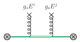
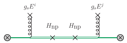
Figure 1: Leading dimension four and six condensate contributions to the Green function. The single and double lines denote the LO color-singlet and color-octet Green functions, respectively. Higher-dimensional corrections are obtained by inserting additional pairs of the non-perturbative Hamiltonian $\hat{H}_{\text{np}}$ in between the two insertions of the chromoelectric dipole $\hat{H}_{D}$.

The first term in (11) is the purely perturbative part. The sum contains the leading non-perturbative contributions, which are proportional to vacuum expectation values of operators of even dimensions and are suppressed by $v^{2}(\Lambda_{\text{QCD}}/(m_{b}v^{2}))^{4,6,8,\dots}$ with respect to the perturbative expression. The contributions of dimension four and six are shown in Figure 1. The extra suppression factor $v^{2}$ is present because terms without at least two insertions of $\hat{H}_{D}$ vanish. The dimension-four correction contains the gluon condensate $\langle\frac{\alpha_{s}}{\pi}G^{2}\rangle$ and has been studied in [23, 24, 25, 26, 4]. The dimension-six correction to the masses and leptonic decay rates of the $\Upsilon(NS)$ resonances has been calculated in [27].

Due to the extra suppression factor $v^{2}$, smallness of the dimension-four contribution is not sufficient to demonstrate the convergence of the expansion in $\Lambda_{\text{QCD}}/(m_{b}v^{2})$ and the calculation of higher-order condensate corrections is necessary to gain more insight. We compute the leading corrections up to dimension eight in Section 2. The NLO potential corrections to the dimension-four condensate contribution are determined in Section 3. The size of the condensate corrections to observables in the $\Upsilon$ system is discussed in Section 4. We conclude in Section 5.

2 Leading order condensate corrections of dimensions four, six and eight

The leading order condensate corrections are finite and can be computed in four dimensions in position space. Inserting spatial integrations, the dimension-four contribution in (11) takes the form

$$\delta_{\Lambda_{\text{QCD}}^{4}}^{(0)}G(E)=O_{0}\int d^{3}\mathbf{r}_{1}\int d^{3}\mathbf{r}_{2}\left(\mathbf{r}_{1}\cdot\mathbf{r}_{2}\right)G_{0}^{(1)}(0,\mathbf{r}_{1};E)G_{0}^{(8)}(\mathbf{r}_{1},\mathbf{r}_{2};E)G_{0}^{(1)}(\mathbf{r}_{2},0;E).$$ (14)

The integrals can be evaluated using the known representations of the LO Green function $G_{0}^{(1,8)}$, where the superscript indicates whether the bottomonium state is in a color singlet $(1)$ or octet $(8)$ configuration. It is convenient to decompose the Green function in terms of partial waves

$$G_{0}^{(1,8)}(\mathbf{r},\mathbf{r}^{\prime};E)=\sum\limits_{l=0}^{\infty}\,(2l+1)\,P_{l}\!\left(\frac{\mathbf{r}\cdot\mathbf{r}^{\prime}}{rr^{\prime}}\right)\,G_{[l]}^{(1,8)}(r,r^{\prime};E),$$ (15)

where $l$ is the quantum number of the angular momentum of the bottom pair and $P_{l}(z)$ are the Legendre polynomials. We use an integral representation from [28],

$$G_{[l]}^{(1,8)}(r,r^{\prime};E)= \hskip 4.26773pt\frac{m_{b}p}{2\pi}\frac{(2pr)^{l}(2pr^{\prime})^{l}}{\Gamma(l+1+\lambda^{(1,8)})\Gamma(l+1-\lambda^{(1,8)})}\,\int\limits_{0}^{1}du\int\limits_{0}^{\infty}dt\left[ut\right]^{l-\lambda^{(1,8)}}$$ (16)

$$\times\left[(1+t)(1-u)\right]^{l+\lambda^{(1,8)}}\exp\left\{-p\,[r^{\prime}(1-2u)+r(1+2t)]\right\},$$

valid for $r^{\prime}<r$ and a sum representation from [29, 24],

$$G_{[l]}^{(1,8)}(r,r^{\prime};E)=\frac{m_{b}p}{2\pi}(2pr)^{l}(2pr^{\prime})^{l}e^{-p(r+r^{\prime})}\sum\limits_{s=0}^{\infty}\frac{s!L_{s}^{(2l+1)}(2pr)L_{s}^{(2l+1)}(2pr^{\prime})}{(s+2l+1)!(s+l+1-\lambda^{(1,8)})},$$ (17)

with the Laguerre polynomials

$$L_{s}^{(\alpha)}(z)=\frac{e^{z}z^{-\alpha}}{s!}\left(\frac{d}{dz}\right)^{s}\left[e^{-z}z^{s+\alpha}\right].$$ (18)

We have defined the variables

$$p=\sqrt{-m_{b}E},\hskip 28.45274pt\lambda^{(1)}=\frac{m_{b}\alpha_{s}C_{F}}{2p},\hskip 28.45274pt\lambda^{(8)}=\frac{m_{b}\alpha_{s}(C_{F}-C_{A}/2)}{2p}.$$ (19)

In the following we take $N_{c}=3$ and use the variable $\lambda\equiv\lambda^{(1)}=-8\lambda^{(8)}$. We use the integral representation (16) for the color-singlet Green functions and the sum representation (17) for the color-octet Green function. The angular integrals in (14) project out the S-wave component of the color-singlet Green functions and the P-wave component of the color-octet Green function. We obtain

$$\delta_{\Lambda_{\text{QCD}}^{4}}^{(0)}G(E)=R_{4}\,\frac{m^{2}\alpha_{s}C_{F}}{4\pi}\,\lambda^{5}\,\sum\limits_{s=0}^{\infty}\frac{s!\,H_{c}(s)^{2}}{(s+3)!(s+2+\lambda/8)},$$ (20)

where

$$R_{4}=\frac{O_{0}}{m_{b}^{4}(\alpha_{s}C_{F})^{6}}=-\frac{\pi^{2}}{18}\;\frac{\langle\frac{\alpha_{s}}{\pi}G^{2}\rangle}{m_{b}^{4}(\alpha_{s}C_{F})^{6}}\,.$$ (21)

The coefficients $H_{c}$ contain the remaining integrations and read

$$H_{c}(s)=\int\limits_{0}^{\infty}dt\left(\frac{1+t}{t}\right)^{\lambda}\int\limits_{0}^{\infty}d\rho\rho^{4}e^{-\rho(1+t)}L_{s}^{(3)}(\rho)=-\frac{(s+3)!}{s!}\lambda\frac{\Gamma(5)\Gamma(s-\lambda)}{\Gamma(5+s-\lambda)}\,.$$ (22)

The sum in (20) yields

$$\delta_{\Lambda_{\text{QCD}}^{4}}^{(0)}G(E) = R_{4}\,\frac{m^{2}\alpha_{s}C_{F}}{4\pi}\,\lambda^{5}\Bigg{\{}\frac{8}{9(8-9\lambda)^{2}(16-9\lambda)^{2}(16+9\lambda)^{2}}\big{(}14155776$$

$$+43024384\lambda+212248576\lambda^{2}-136918656\lambda^{3}-607347072\lambda^{4}$$

$$+444623094\lambda^{5}+321157305\lambda^{6}-245939085\lambda^{7}-47534445\lambda^{8}$$

$$+37200870\lambda^{9}\big{)}+\left(\psi_{1}(\lambda)-\frac{\pi^{2}}{\sin^{2}(\pi\lambda)}\right)$$

$$\times\frac{16\lambda^{2}\left(26624-101216\lambda^{2}+109935\lambda^{4}-25515\lambda^{6}\right)}{16384-25920\lambda^{2}+6561\lambda^{4}}$$

$$+\frac{134217728\lambda\left(64-\lambda^{2}\right)}{9\left(16384-25920\lambda^{2}+6561\lambda^{4}\right)^{2}}\left(\psi(1-\lambda)-\psi\left(2+\frac{\lambda}{8}\right)\right)\Bigg{\}},$$

where $\psi$ and $\psi_{1}$ are the polygamma functions of order 0 and 1, respectively. The condensate corrections to the S-wave energy levels $E_{N}$ and the wave functions at the origin $|\psi_{N}(0)|^{2}$ can be obtained from the expansion of (2) for $\lambda$ near positive integer values $N$ as described e.g. in [30, 31, 20]. The results are given in Appendix A.

The same strategy can be applied for the calculation of the dimension six and eight condensate corrections. Again, the angular integrals project out the S-wave component of the color-singlet Green functions and the P-wave components of the color-octet Green functions. We find

$$\delta_{\Lambda_{\text{QCD}}^{6}}^{(0)}G(E) = R_{6}\frac{m^{2}\alpha_{s}C_{F}}{4\pi}\lambda^{9}\sum\limits_{s_{1}=0}^{\infty}\sum\limits_{s_{2}=0}^{\infty}\sum\limits_{s_{3}=0}^{\infty}\frac{s_{1}!H_{c}(s_{1})}{(s_{1}+3)!(s_{1}+2+\lambda/8)}$$ (24)

$$\frac{K_{c}(s_{1},s_{2})\,s_{2}!\,K_{c}(s_{2},s_{3})}{(s_{2}+3)!(s_{2}+2+\lambda/8)}\frac{s_{3}!H_{c}(s_{3})}{(s_{3}+3)!(s_{3}+2+\lambda/8)},$$

and

$$\delta_{\Lambda_{\text{QCD}}^{8}}^{(0)}G(E) = R_{8}\frac{m^{2}\alpha_{s}C_{F}}{4\pi}\lambda^{13}\sum\limits_{i=1}^{5}\sum\limits_{s_{i}=0}^{\infty}\frac{s_{1}!H_{c}(s_{1})}{(s_{1}+3)!(s_{1}+2+\lambda/8)}\frac{s_{5}!H_{c}(s_{5})}{(s_{5}+3)!(s_{5}+2+\lambda/8)}$$ (25)

$$\times\frac{K_{c}(s_{1},s_{2})s_{2}!K_{c}(s_{2},s_{3})s_{3}!K_{c}(s_{3},s_{4})s_{4}!K_{c}(s_{4},s_{5})}{(s_{2}+3)!(s_{2}+2+\lambda/8)(s_{3}+3)!(s_{3}+2+\lambda/8)(s_{4}+3)!(s_{4}+2+\lambda/8)},$$

where

$$R_{6}=\frac{O_{1}}{m_{b}^{6}(\alpha_{s}C_{F})^{10}},\hskip 42.67912ptR_{8}=\frac{O_{2}}{m_{b}^{8}(\alpha_{s}C_{F})^{14}},$$ (26)

and the coefficients $K_{c}$ read

$$K_{c}(a,b) = \int\limits_{0}^{\infty}d\rho\rho^{4}e^{-\rho}L_{a}^{(3)}(\rho)L_{b}^{(3)}(\rho)$$ (27)

$$= \frac{(\text{max}(a,b)+3)!}{\text{min}(a,b)!}\left[(2a+4)\delta_{a,b}-\delta_{a,b-1}-\delta_{a-1,b}\right].$$

Since $K_{c}(a,b)$ is only non-vanishing for $|a-b|\leq 1$ the multiple sums in (24) and (25) are reduced to a single sum, which can be solved in terms of polygamma functions. The lengthy results are available as ancillary files with the arXiv version of this article. The dimension six and eight contributions to the energy levels and wave functions are given in Appendix A.

3 Dimension four contribution at NLO: Potential contributions

The NLO corrections to the dimension-four condensate contribution involve an insertion of the NLO Coulomb potential as shown in Figure 2 and ultrasoft loops as shown in Figure 3. The upper panel of Figure 3 shows the diagrams with ultrasoft gluon loops, where the gluon coupling to the color-octet state originates from the leading term $g_{s}A_{0}^{\text{us}}(t,\mathbf{0})$ in the multipole expansion. The equivalent coupling to the color singlet state vanishes because the ultrasoft gluons cannot resolve the spatial separation of the bottom-antibottom state and the net color charge vanishes in the singlet state. The diagram in the lower panel of Figure 3 shows the contribution from the light-quark condensate $\langle\bar{q}q\rangle$ with $q=u,d,s$ which is also counted as dimension four because, due to chirality suppression, the quark condensate $\langle\bar{q}q\rangle$ only appears together with one power of the light quark mass $m_{q}$ which is of the order $\Lambda_{\text{QCD}}$. There is a number of other effects that could possibly contribute at that order:

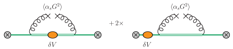
Figure 2: Potential corrections to the dimension four condensate contribution to the Green function.

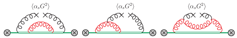
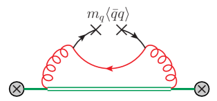
Figure 3: Corrections to the dimension four condensate contribution to the Green function involving ultrasoft loops. Lines that carry ultrasoft momentum are drawn in red.

• An $\alpha_{s}$ correction to the Wilson coefficient of the chromoelectric dipole operator (4). The Wilson coefficient was found to be trivial up to $\mathcal{O}(\alpha_{s}^{2})$ in [33].

• $\mathcal{O}(m_{b}^{2}v^{3}\Lambda_{\text{QCD}}^{2})$ terms in the multipole expansion (4) of the gluon coupling to bottom quarks in the spatial components. They are identical to the multipole expansion of the coupling to the ultrasoft gluon field and were determined in [34], where they are denoted as $h_{SO}^{(1,0)}$. There is no NLO contribution from these terms because they either have vanishing tree level Wilson coefficients and are thus suppressed by an additional power of $\alpha_{s}\sim v$ or involve the chromomagnetic instead of the chromoelectric field, which only yields a vanishing condensate $\Braket{0}{E_{i}^{A}B_{j}^{B}}{0}=0$ at NLO.

• Contrary to the ultrasoft gluon-bottom coupling, the interactions of the non-perturbative gluon field must also be multipole expanded in the time component. The expansion of the $A^{0}$ component is trivial due to our gauge choice (3) and already the linear term $t(\partial^{0}A^{i})(0,\mathbf{0})$ in the expansion of the spatial component is only relevant at higher powers. Thus, no contributions of this type need to be considered at NLO.

The potential corrections are determined below, whereas the ultrasoft contribution is postponed to future work. The NLO correction to the Coulomb potential is given by

$$\delta^{(1)}V^{(1,8)}(\mathbf{q})=\frac{\alpha_{s}^{2}\,C^{(1,8)}}{\mathbf{q}^{2}}\,\left\{\left[\left(\frac{\mu^{2}}{\mathbf{q}^{2}}\right)^{\epsilon}-1\right]\frac{\beta_{0}}{\epsilon}+\left(\frac{\mu^{2}}{\mathbf{q}^{2}}\right)^{\epsilon}a_{1}(\epsilon)\right\}\,,$$ (28)

where the color factors are given by $C^{(1)}=-C_{F}$ and $C^{(8)}=C_{A}/2-C_{F}$ and

$$a_{1}(\epsilon) = \Big{(}C_{A}[11-8\epsilon]-4T_{F}n_{f}\Big{)}\frac{e^{\gamma_{E}\epsilon}\Gamma(1-\epsilon)\Gamma(2-\epsilon)\Gamma(\epsilon)}{(3-2\epsilon)\Gamma(2-2\epsilon)}-\frac{\beta_{0}}{\epsilon},$$

$$\beta_{0} = \frac{11C_{A}}{3}-\frac{4T_{F}n_{f}}{3},$$ (29)

where $n_{f}$ is the number of massless quarks. Denoting the contribution from the left (right) diagram in Figure 2 by DVD (DDV), we find

$$\delta_{\Lambda_{\text{QCD}}^{4}}^{(1),\text{ pot}}G(E) = \delta_{\Lambda_{\text{QCD}}^{4}}^{(1),\;\text{DVD}}G(E)+2\,\delta_{\Lambda_{\text{QCD}}^{4}}^{(1),\,\text{DDV}}G(E)$$

$$= -O_{0}\,\alpha_{s}^{2}\,\left[a_{1}+\beta_{0}\frac{d}{du}\right]$$

$$\left[\left(\frac{C_{A}}{2}-C_{F}\right)I_{\Lambda_{\text{QCD}}^{4}}[D,1+u,D]+\,2\,(-C_{F})\,I_{\Lambda_{\text{QCD}}^{4}}[D,D,1+u]\right]_{u=0}.$$

The first triple insertion function takes the form

$$I_{\Lambda_{\text{QCD}}^{4}}[D,1+u,D] = \frac{\mu^{2u}}{4\pi\Gamma(1+2u)\cos(\pi u)}\int d^{3}\mathbf{r}_{1}\int d^{3}\mathbf{r}_{2}\int d^{3}\mathbf{r}_{3}\,(\mathbf{r}_{1}\cdot\mathbf{r}_{3})$$ (31)

$$\times G_{0}^{(1)}(0,\mathbf{r}_{1};E)G_{0}^{(8)}(\mathbf{r}_{1},\mathbf{r}_{2};E)r_{2}^{-1+2u}G_{0}^{(8)}(\mathbf{r}_{2},\mathbf{r}_{3};E)G_{0}^{(1)}(\mathbf{r}_{3},0;E)$$

$$= \frac{\lambda^{6}}{(4\pi)^{2}m_{b}^{2}(\alpha_{s}C_{F})^{6}}\sum\limits_{s_{1}=0}^{\infty}\sum\limits_{s_{2}=0}^{\infty}\frac{s_{1}!H_{c}(s_{1})}{(s_{1}+3)!(s_{1}+2+\lambda/8)}$$

$$\times K_{V}(u,s_{1},s_{2})\,\frac{s_{2}!H_{c}(s_{2})}{(s_{2}+3)!(s_{2}+2+\lambda/8)},$$

where

$$K_{V}(u,s_{1},s_{2})=\frac{(\mu/2p)^{2u}}{\Gamma(1+2u)\cos(\pi u)}\int\limits_{0}^{\infty}d\rho\rho^{3+2u}e^{-\rho}L_{s_{1}}^{(3)}(\rho)L_{s_{2}}^{(3)}(\rho).$$ (32)

The full $u$-dependence of (32) is not needed here. To evaluate (3) we only need the value and the first derivative at $u=0$. We obtain

$$K_{V}^{(0)}(s_{1},s_{2})\equiv K_{V}(0,s_{1},s_{2})=\frac{(s_{1}+3)!}{s_{1}!}\delta_{s_{1}s_{2}}.$$ (33)

The derivative of (32) at zero can be solved by applying the methods used for the Coulomb triple insertion in [30]. This yields

$$K_{V}^{(1)}(s_{1},s_{2})\equiv\frac{d}{du}K_{V}(u,s_{1},s_{2})|_{u=0}=2\left[(L_{\lambda}+\gamma_{E})\frac{(s_{1}+3)!}{s_{1}!}\delta_{s_{1}s_{2}}+k_{V}(s_{1},s_{2})\right],$$ (34)

where $L_{\lambda}=\ln(\lambda\mu/(m_{b}\alpha_{s}C_{F}))$ and

$$k_{V}(s_{1},s_{2})=\begin{cases}11+12s_{1}+3s_{1}^{2}+\frac{(s_{1}+3)!}{s_{1}!}\psi(1+s_{1}),&s_{1}=s_{2}\\ -\frac{(\text{min}(s_{1},s_{2})+3)!}{\text{min}(s_{1},s_{2})!|s_{1}-s_{2}|},&\text{else.}\end{cases}$$ (35)

The second triple-insertion function yields

$$I_{\Lambda_{\text{QCD}}^{4}}[D,D,1+u] = \frac{\mu^{2u}}{4\pi\Gamma(1+2u)\cos(\pi u)}\int d^{3}\mathbf{r}_{1}\int d^{3}\mathbf{r}_{2}\int d^{3}\mathbf{r}_{3}\,(\mathbf{r}_{1}\cdot\mathbf{r}_{2})$$ (36)

$$\times G_{0}^{(1)}(0,\mathbf{r}_{1};E)G_{0}^{(8)}(\mathbf{r}_{1},\mathbf{r}_{2};E)G_{0}^{(1)}(\mathbf{r}_{2},\mathbf{r}_{3};E)r_{3}^{-1+2u}G_{0}^{(1)}(\mathbf{r}_{3},0;E)$$

$$= \frac{\lambda^{6}}{(4\pi)^{2}m_{b}^{2}(\alpha_{s}C_{F})^{6}}\sum\limits_{s_{1}=0}^{\infty}\sum\limits_{s_{2}=0}^{\infty}\frac{s_{1}!H_{c}(s_{1})}{(s_{1}+3)!(s_{1}+2+\lambda/8)}$$

$$\times K_{D}(s_{1},s_{2})\,\frac{H(u,s_{2}+1)}{(s_{2}+1)(s_{2}+1-\lambda)},$$

where

$$K_{D}(s_{1},s_{2}) = \int\limits_{0}^{\infty}d\rho\rho^{4}e^{-\rho}L_{s_{1}}^{(3)}(\rho)L_{s_{2}}^{(1)}(\rho)$$ (37)

$$= \begin{cases}(-1)^{s_{1}+s_{2}}4!\frac{(s_{1}+3)!}{s_{2}!(s_{1}+3-s_{2})!}\frac{(s_{2}+1)!}{s_{1}!(s_{2}+1-s_{1})!},&-1\leq s_{2}-s_{1}\leq 3\\ 0,&\text{else,}\end{cases}$$

and $H(u,k)$ is defined as in [30]. Also here, we only need the value and the first derivative at $u=0$:

$$H^{(0)}(k) \equiv H(0,k)=\frac{k}{k-\lambda},$$ (38)

$$H^{(1)}(k) \equiv \frac{\partial}{\partial u}H(u,k)|_{u=0}$$ (39)

$$= \frac{2k}{k-\lambda}\left[L_{\lambda}-\gamma_{E}-\psi(k-\lambda)+\frac{\lambda}{k}\left(\psi(1-\lambda)-\psi(k+1-\lambda)\right)\right].$$

The infinite sums in (31) and (36) converge quickly and can be truncated with negligible uncertainty at $s_{i}\sim 30$ for the numerical evaluation of the Green function. The contributions to the energy levels and wave functions from the potential corrections can be extracted by expanding (31) and (36) for $\lambda$ near positive integer values $N$. The results are given in Appendix A.

4 Phenomenology of condensate corrections

The size of non-perturbative corrections to the moments and to the properties of the $\Upsilon$ resonances has been strongly disputed for various reasons. First, the assumption $\Lambda_{\text{QCD}}\ll m_{b}v^{2}$ is questionable and is certainly only valid for a limited number of observables in the $\Upsilon$ system. Here, we perform an unbiased analysis of the expansion in terms of local condensates and assess the validity based on its convergence. The breakdown of this expansion is a clear indication that the above assumption is inappropriate.

Furthermore, the numerical values of the local condensates are very uncertain. The condensate $O_{0}$ is proportional to the gluon condensate and we will use the standard value $\langle\frac{\alpha_{s}}{\pi}G^{2}\rangle^{\text{SVZ}}=0.012\text{\,GeV}^{4}$ from [35] below, unless indicated otherwise. We note however, that significantly larger values have also been obtained in the literature, see e.g. [36, 37]. Clearly, the situation is even more uncertain for the higher-dimensional condensates. Since our main objective is the assessment of the convergence properties, we rely on naive rescaling

$$O_{0}^{\text{SVZ}}=-(285\text{\,MeV})^{4},\hskip 28.45274ptO_{1}^{\text{naive}}=(285\text{\,MeV})^{6},\hskip 28.45274ptO_{2}^{\text{naive}}=-(285\text{\,MeV})^{8}.$$ (40)

The value of $O_{0}$ is scale independent since the gluon condensate $\langle\frac{\alpha_{s}}{\pi}G^{2}\rangle$ is not renormalized. We neglect the scale dependence of the higher-dimensional condensates which is very weak compared to that of the coefficients which contain large powers of $\alpha_{s}$. The estimate $O_{1}^{\text{naive}}$ is in good agreement with the result of [27], where an expression for $O_{1}$ in terms of the dimension-six gluon condensate $\langle G^{3}\rangle$ and the quark-condensate $\langle\bar{q}q\rangle$ has been derived based on the factorization hypothesis. The analysis of [27] also shows that $O_{1}$ is only weakly scale dependent.

In addition, the corrections to the masses and leptonic decay rate depend strongly on the renormalization scale, because large powers of $\alpha_{s}$ appear in the ratios (21) and (26). The fact that different powers of $\alpha_{s}$ appear in the contributions of different dimensions also complicates the assessment of the convergence and different conclusions have been drawn based on different scale choices. We distinguish the scale $\mu_{c}$, used in the condensate corrections, from the renormalization scale $\mu$ in the perturbative contribution. The main motivation for the calculation of the potential corrections to the dimension-four contribution has been to gain more insight into the appropriate scale choice for $\mu_{c}$ by considering the convergence of the perturbative series. We note that the potential corrections contain all logarithms $\ln(\mu_{c})$ that are required to cancel the $\mu_{c}$ dependence of the dimension-four contribution at NLO. The ultrasoft correction must therefore be free of logarithms $\ln(\mu_{c})$ and is less scale dependent, which justifies performing this analysis based on incomplete NLO corrections. Scales below 0.8 GeV are not considered below, because the value of $\alpha_{s}$ and perturbation theory in general become unreliable in this regime.

4.1 The $\Upsilon(1S)$ mass

First, we briefly review the status of the purely perturbative prediction for the mass of the $\Upsilon(1S)$ resonance. We use QQbar_Threshold [38, 20] in the PS mass scheme [39] with the input value $m_{b}^{\text{PS}}=4.532_{-0.039}^{+0.013}\text{\,GeV}$ from [5, 6]. The effects of a non-zero charm-quark mass are included up to NNLO [5] using the mass $\overline{m}_{c}(3\text{\,GeV})=993\text{\,MeV}$ from [40, 41]. The default values of QQbar_Threshold are taken for the strong coupling $\alpha_{s}(m_{Z})=0.1184\pm 0.0010$ and all other parameters, and QED corrections are taken into account with NNLO accuracy. The result is shown in the top panel of Figure 4. We observe that the convergence is best for scales that are considerably larger than the soft scale $\mu\sim m_{b}\alpha_{s}(\mu)C_{F}$. This has motivated the authors of [11] to choose a central scale of 5.35 GeV, which is significantly larger than that of [9, 10, 12] (2.5 and 1.9 GeV, respectively) and leads to a much smaller estimate for the perturbative uncertainty. Here, we choose a central scale of 3 GeV such that a variation by factors 1/2 and 2 covers the choices of [9, 10, 11, 12]. The perturbative expansion takes the form

$$M_{\Upsilon(1S)}^{\text{pert}}\,(3\text{\,GeV})=(9\,366+82+4-27)\text{\,MeV}.$$ (41)

In addition to the perturbative uncertainty from scale variation, we also take into account the parametric uncertainty from the bottom-quark PS mass and we use the size of the charm-quark mass effects up to NNLO as an estimate for the missing NNNLO correction. The parametric uncertainty from the strong coupling is small in the PS mass scheme and is neglected.

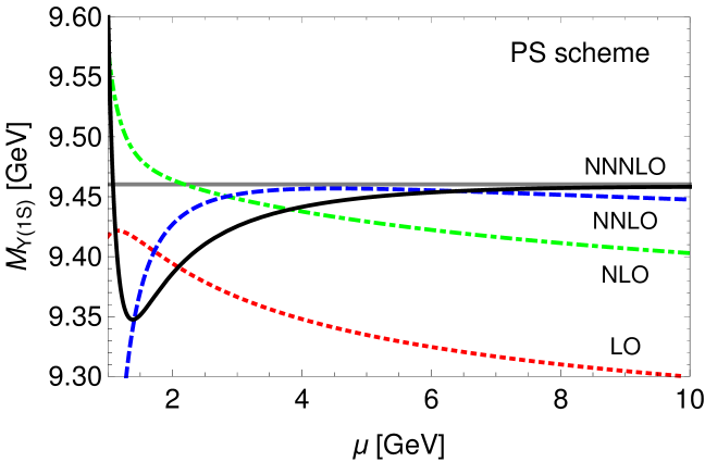
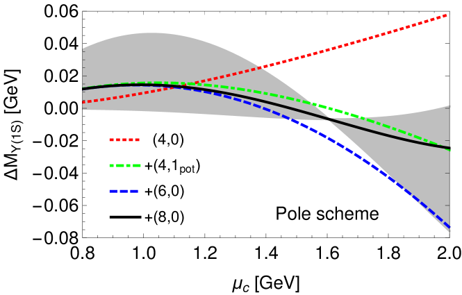
Figure 4: The top panel shows the perturbative contribution to the mass of the $\Upsilon(1S)$ resonance. The curves in the bottom panel show the effects of cumulatively adding the condensate contributions $(i,j)$ where $i$ denotes the dimension and $j$ the order in perturbation theory. The gray band is spanned by variation of $O_{0}$ by factors of 0 and 3, while $O_{1}$ and $O_{2}$ are unchanged.

The condensate corrections with the values of (40) are shown in the lower panel of Figure 4. At the considered orders, the mass scheme is ambiguous and we use the one-loop pole mass in the condensate contribution. In the PS scheme, the condensate contributions are slightly enhanced and the convergence is slightly worsened but the overall conclusions are unchanged. We observe that the potential corrections to the dimension-four condensate contribution stabilize the behaviour under scale variation and show a clear preference for rather small scales around $\mu_{c}=1.2\text{\,GeV}$, which we take as the central value. The condensate contribution takes the form

$$\Delta M_{\Upsilon(1S)}^{\text{cond}}\,(1.2\text{\,GeV})=\left[(17-3)\,\frac{O_{0}}{O_{0}^{\text{SVZ}}}-4\,\frac{O_{1}}{O_{1}^{\text{naive}}}+1\,\frac{O_{2}}{O_{2}^{\text{naive}}}\right]\text{\,MeV}.$$ (42)

The grey band in Figure 4 is obtained by varying the value of the condensate $O_{0}$ between 0 GeV⁴ and $3O_{0}^{\text{SVZ}}$. In our analysis the condensates of dimension six and eight are varied between 0 GeV⁶ and $3^{3/2}O_{1}^{\text{naive}}$, and 0 GeV⁸ and $3^{2}O_{2}^{\text{naive}}$, respectively. We use this variation at the central scale as an estimate for the uncertainty from the value of the condensates.

The condensate expansion becomes unstable near $\mu_{c}\approx 2\,\text{GeV}$ where the LO dimension four, six and eight contributions are all of the same size. The variation of $\mu_{c}$ between 0.8 GeV and 2 GeV yields an uncertainty of ${}_{-36}^{+3}$ MeV. We take $\pm 36$ MeV as an estimate for the perturbative uncertainty in order to also account for the unknown ultrasoft NLO correction. Combining the perturbative and condensate contributions we find

$$M_{\Upsilon(1S)} = 9\,437\,_{-114}^{+61}\text{ MeV}$$ (43)

$$= 9\,437\,_{-74}^{+28}\,(\mu)\,_{-75}^{+25}\,(m_{b})\,_{-1}^{+0}\,(\alpha_{s})\,\pm 9\,(m_{c})$$

$$\pm 36\,(\mu_{c})\,_{-14}^{+29}\,(O_{0})\,_{-18}^{+4}\,(O_{1})\,_{-1}^{+10}\,(O_{2})\text{ MeV},$$

which is in good agreement with the experimental value $M_{\Upsilon(1S)}^{\text{exp}}=9\,460.30\pm 0.26$ MeV.

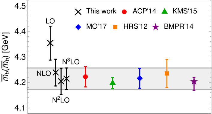
Figure 5: Comparison of our result for the bottom-quark $\overline{\text{MS}}$ mass from $M_{\Upsilon(1S)}$ with other recent results from the masses of $b\bar{b}$ bound states (ACP’14 [9, 10], KMS’15 [11], MO’17 [12]) and non-relativistic sum rules (HRS’12 [8], BMPR’14 [5, 6]). The bottom-quark masses obtained from lower orders in pure perturbation theory, while retaining all known condensate contributions, are shown as well. The order of the PS-$\overline{\text{MS}}$ mass relation has been correlated with the order in perturbation theory.

The stable behaviour of the condensate corrections in the range $0.8\,\text{GeV}\lesssim\mu_{c}\lesssim 2\,\,\text{GeV}$ facilitates the determination of the bottom-quark mass from the experimental value of the $\Upsilon(1S)$ mass. We obtain

$$m_{b}^{\text{PS}}(2\,\text{GeV})=4544\pm 39\,(\text{pert.})\,_{-25}^{+22}\,(\text{non-pert.})\text{ MeV}=4544\,_{-46}^{+44}\text{ MeV},$$ (44)

where we have symmetrized the uncertainty from variation of the renormalization scale $\mu$, by taking the maximum of the positive and negative error. The perturbative uncertainty is obtained by adding the errors from variation of $\mu$ and $\alpha_{s}$ as well as our estimate of higher-order charm-quark mass effects in quadrature. The variation of the scale $\mu_{c}$ and of the values of the condensates is combined into the non-perturbative uncertainty. The result (44) is converted to the $\overline{\text{MS}}$ scheme at NNNLO [42, 43] using QQbar_Threshold. We distinguish the scale $\mu_{m}$ used in the conversion, which is set to $m_{b}^{\text{PS}}$, and estimate the uncertainty through variation of $\mu_{m}$ by factors of 1/2 and 2 and symmetrization as described above. We find

$$\overline{m}_{b}(\overline{m}_{b})=4214\pm 37\,(\text{pert.})\,_{-22}^{+20}\,(\text{non-pert.})\text{ MeV}=4214\,_{-43}^{+42}\text{ MeV}.$$ (45)

The result shows good convergence and agrees with other recent determinations of $m_{b}$ from the data on the $\Upsilon$ system as shown in Figure 5. In conclusion, our analysis demonstrates that the determination of the bottom-quark mass from the $\Upsilon(1S)$ mass is possible with a total uncertainty of the order of $\pm$45 MeV. It should however be noted that this approach to the determination of the bottom-quark mass is on a less sound footing theoretically than the extraction based on non-relativistic moments with $n\approx 10$, which are discussed in Section 4.4.

4.2 The $\Upsilon(2S)$ mass

We repeat the above discussion for the $\Upsilon(2S)$ mass. The scale dependence of the perturbative result is shown in Figure 6. Since the soft scale is lower for the $n=2$ states, we reduce the central scale to 2 GeV, where the perturbative series takes the form

$$M_{\Upsilon(2S)}^{\text{pert}}\,(2\text{\,GeV})=(9\,534+198+154+116)\text{\,MeV}.$$ (46)

As the plot shows, the convergence is rather slow, independently of the choice of scale. We also note that the charm-mass effects at NNLO are +39 MeV and significantly larger than for the $\Upsilon(1S)$ mass (+8 MeV). As we argued in [5], the charm-mass effects are a measure for the IR sensitivity of an observable. Thus, the significantly larger value is an indication that the non-perturbative correction should be considerably larger and less convergent for the $\Upsilon(2S)$ mass than for the the $\Upsilon(1S)$ mass.

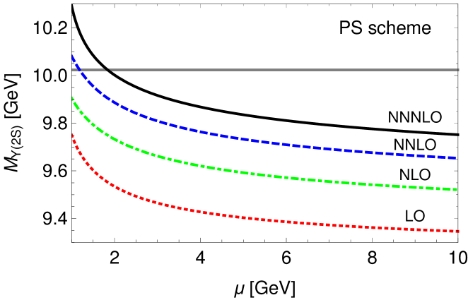
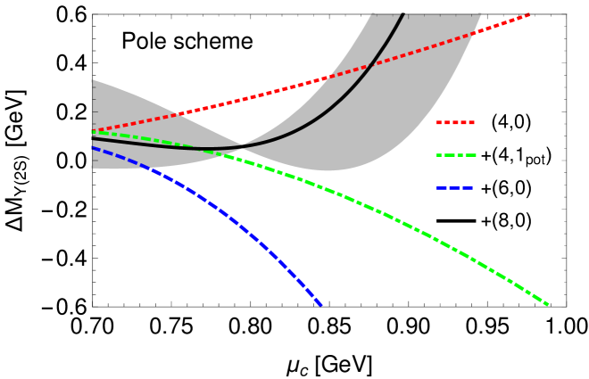
Figure 6: The top panel shows the perturbative contribution to the mass of the $\Upsilon(2S)$ resonance. The curves in the bottom panel show the effects of cumulatively adding the condensate contributions $(i,j)$ where $i$ denotes the dimension and $j$ the order in perturbation theory. The gray band is spanned by variation of $O_{0}$ by factors of 0 and 3, while $O_{1}$ and $O_{2}$ are unchanged.

Turning to the condensate corrections, which are shown in the lower panel of Figure 6, we can confirm this expectation. The expansion already breaks down for $\mu_{c}=0.8$ GeV, where the individual contributions are

$$\Delta M_{\Upsilon(2S)}^{\text{cond}}\,(0.8\text{\,GeV})=\left[(258-267)\,\frac{O_{0}}{O_{0}^{\text{SVZ}}}-293\,\frac{O_{1}}{O_{1}^{\text{naive}}}+365\,\frac{O_{2}}{O_{2}^{\text{naive}}}\right]\text{\,MeV}.$$ (47)

At lower scales, the use of perturbation theory cannot be justified. Thus, while we cannot rule out the convergence of the local condensate expansion unambiguously due to the large uncertainties of the $O_{i}$, clearly no reliable prediction for the non-perturbative contribution can be obtained like this.

A more promising approach to the $\Upsilon(2S)$ mass is to assume the hierarchy $\Lambda_{\text{QCD}}\sim m_{b}v^{2}\ll m_{b}v$. Then, the ultrasoft contribution takes the form of a non-local condensate instead of a perturbative correction [15, 44, 45]. This implies that the leading non-perturbative correction is of the order

$$\Delta M_{\Upsilon(2S)}^{\text{non-perturbative}}\sim m_{b}\alpha_{s}^{2}\times\left(\frac{\Lambda_{\text{QCD}}}{m_{b}\alpha_{s}}\right)^{2}\times\rho\left(\frac{\Lambda_{\text{QCD}}}{m_{b}\alpha_{s}^{2}}\right)\sim m_{b}\alpha_{s}^{4},$$ (48)

which is formerly of NNLO, and the conclusion that the local condensate expansion breaks down is equivalent to the statement that the $\Upsilon(2S)$ system is outside the radius of convergence for the presently unknown function $\rho$. In this scenario, the perturbative NNNLO results, which contain the perturbative evaluation of the ultrasoft contribution cannot be used and we have to resort to the NNLO expressions. The result for the $\Upsilon(2S)$ mass reads

$$M_{\Upsilon(2S)}=9\,886\,_{-122}^{+195}\,(\mu)\,_{-76}^{+25}\,(m_{b})\,_{-26}^{+28}\,(\alpha_{s})\pm\mathcal{O}(100)\,(\text{non-pert.})\text{ MeV},$$ (49)

where the estimate for the non-perturbative contributions follows from the assumption that the function $\rho$ in (48) is of order one. Within the large uncertainty, the experimental value $M_{\Upsilon(2S)}^{\text{exp}}=10023.26\pm 0.31$ MeV can be reproduced.

4.3 The $\Upsilon(1S)\to l^{+}l^{-}$ decay width

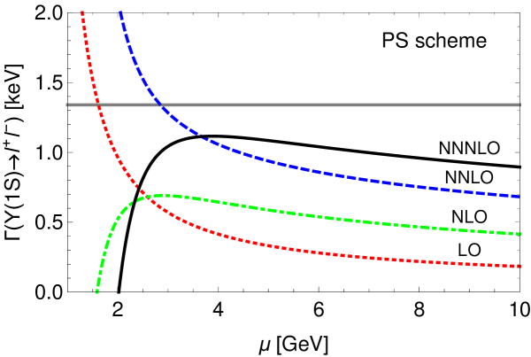
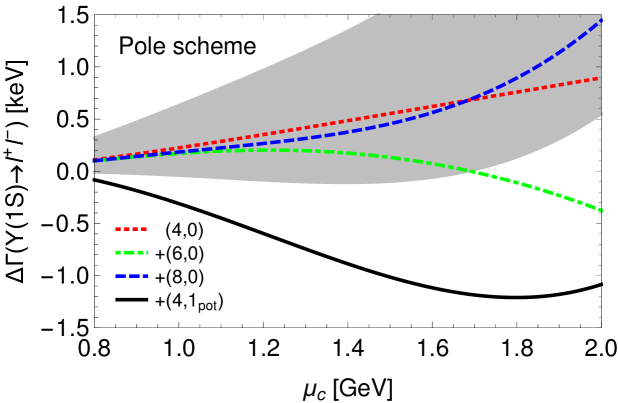
Figure 7: The top panel shows the perturbative contribution to the leptonic decay width of the $\Upsilon(1S)$ resonance. The curves in the bottom panel show the effects of cumulatively adding the condensate contributions $(i,j)$ where $i$ denotes the dimension and $j$ the order in perturbation theory. The gray band is spanned by variation of $O_{0}$ by factors of 0 and 3, while $O_{1}$ and $O_{2}$ are unchanged. In this Figure the gray band does not contain the potential corrections to the dimension-four contribution.

The perturbative NNNLO result for the leptonic decay width of the $\Upsilon(1S)$ resonance has been obtained in [4]. Here, we repeat their analysis including charm-mass effects up to NNLO, which increase the leptonic width by 0.03 keV. The scale dependence is shown in Figure 7 and we adopt 3.5 GeV as the central scale. The perturbative series stabilizes at NNNLO

$$\Gamma^{\text{pert}}(\Upsilon(1S)\to l^{+}l^{-})\,(3.5\,\text{GeV})=\frac{4\pi\alpha^{2}}{9m_{b}^{2}}\,c_{v}\left[c_{v}-\left(c_{v}+\frac{d_{v}}{3}\right)\,\frac{E_{1}}{m_{b}}\right]\left|\psi_{1}(0)\right|^{2}$$ (50)

$$= (0.48+0.19+0.47-0.04)\,\text{keV}=1.11\,_{-0.22}^{+0.07}\,\text{keV}$$

$$= 1.11\,_{-0.21}^{+0.01}\,(\mu)\pm\,0.00(m_{b})\pm\,0.04(m_{c})\pm\,0.05(\alpha_{s})\,\text{keV}$$

but falls short of the experimental value $\Gamma^{\text{exp}}(\Upsilon(1S)\to l^{+}l^{-})=1.340\pm 0.018$ keV by about 20%. Following [4] we determine the scale uncertainty from variation between 3 and 10 GeV. The other input parameters are varied as above.

The condensate contributions are shown in the lower panel of Figure 7. Using the same central scale $\mu_{c}=1.2$ GeV as for the $\Upsilon(1S)$ mass, we obtain

$$\Gamma^{\text{cond}}(\Upsilon(1S)\to l^{+}l^{-})\,(1.2\text{\,GeV})=\left[(352-862)\,\frac{O_{0}}{O_{0}^{\text{SVZ}}}-149\,\frac{O_{1}}{O_{1}^{\text{naive}}}+64\,\frac{O_{2}}{O_{2}^{\text{naive}}}\right]\text{\,eV}.$$ (51)

Focusing first on the leading-order contributions, we see that the expansion converges and yields a contribution of 0.27 keV that closes the difference between the perturbative and the experimental value. Compared to the $\Upsilon(1S)$ mass the expansion breaks down at a smaller scale around 1.6 GeV.

However, with the addition of the potential corrections to the dimension four contribution, the agreement is destroyed. The potential correction already exceeds the LO term at the scale 0.7 GeV and becomes twice as large at 0.9 GeV. This apparent breakdown of the perturbative series makes it impossible to give a reliable estimate of the non-perturbative contribution. However, it is conceivable that the large potential corrections are compensated by the missing ultrasoft correction, thus stabilizing the perturbative expansion of the dimension-four contribution. Therefore, no definite conclusions about the validity of the local condensate expansion for $\Gamma(\Upsilon(1S)\to l^{+}l^{-})$ can be drawn without a calculation of the full NLO corrections to the dimension-four contribution.

4.4 The non-relativistic moments

The moments ${\cal M}_{n}$ of the normalized inclusive $b\bar{b}$ production cross section

$$R_{b}(s)=\frac{\sigma(e^{+}e^{-}\to b\overline{b}+X)}{\sigma(e^{+}e^{-}\to\mu^{+}\mu^{-})}\,,$$ (52)

in $e^{+}e^{-}$ collisions with the center-of-mass energy $s$, are defined as

$${\cal M}_{n}\equiv\int_{0}^{\infty}ds\,\frac{R_{b}(s)}{s^{n+1}}=-6\pi i\oint_{{\cal C}}ds\,\frac{\Pi_{b}(s)}{s^{n+1}}=\frac{12\pi^{2}}{n!}\bigg{(}\frac{d}{dq^{2}}\bigg{)}^{n}\Pi_{b}\big{(}q^{2}\big{)}\bigg{|}_{q^{2}=0}\,.$$ (53)

The normalized cross section is related to the bottom-quark contribution $\Pi_{b}$ to the photon vacuum polarization by the optical theorem $R_{b}(s)=12\pi\operatorname{Im}\Pi_{b}(s+i\epsilon)$. The contour ${\cal C}$ must be closed around $s=0$ without crossing the branch cut for real $s\geq M_{\Upsilon(1S)}^{2}$. The perturbative contributions to the moments up to NNNLO have been discussed in detail in [5]. The non-perturbative corrections can be determined by inserting the condensate contribution to the cross section

$$\Pi_{b}^{\text{cond}}(s) = \frac{2N_{c}e_{b}^{2}}{s}\,\Bigg{[}\delta_{\Lambda_{\text{QCD}}^{4}}^{(0)}G(E)+\left(2c_{v}^{(1)}\,\frac{\alpha_{s}}{4\pi}\,\delta_{\Lambda_{\text{QCD}}^{4}}^{(0)}G(E)+\delta_{\Lambda_{\text{QCD}}^{4}}^{(1),\text{pot}}G(E)\right)$$ (54)

$$\hskip 36.98866pt+\delta_{\Lambda_{\text{QCD}}^{6}}^{(0)}G(E)+\delta_{\Lambda_{\text{QCD}}^{8}}^{(0)}G(E)+\dots\Bigg{]}\,,$$

where $E=\sqrt{s}-2m_{b}$ and $c_{v}^{(1)}=-8C_{F}$ is the hard matching coefficient of the vector current, into (53). Following the discussion in [5] we choose not to expand the prefactor $1/s$ around $1/(4m_{b}^{2})$. Contrary to the perturbative contribution, we cannot split the condensate corrections into a resonance and continuum part, since both are separately divergent [5]. The total corrections to the moments are however well-defined and can be computed numerically using the representation of the moments (53) involving contour integration or, in principle, analytically by taking derivatives at $q^{2}=0$.

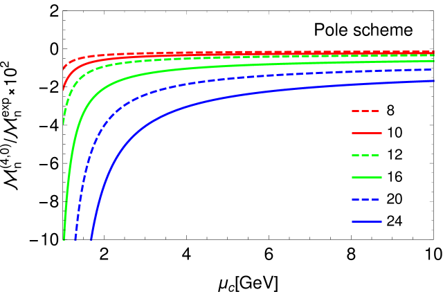
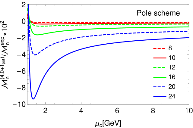
Figure 8: Dimension-four corrections to various non-relativistic moments relative to the experimental moments from [5]. The upper panel shows the leading order contribution and the lower panel the leading order contribution plus the potential corrections. The relative corrections have been rescaled by a factor of 100.

The scale dependence of the dimension-four contribution are shown in Figure 8. Results are given in the pole mass scheme using the same inputs as given above. We refrain from using the PS or other threshold mass schemes, because the perturbative expansion in these schemes becomes unstable in large regions of the scale $\mu_{c}$. This can be traced back to the appearance of large powers of $\lambda$ in the expression for the Green function (2), which are expanded in the PS mass scheme as

$$\lambda^{k}=\left(\frac{m_{b}^{\text{PS}}\alpha_{s}C_{F}}{2\sqrt{-m_{b}^{\text{PS}}E^{\text{PS}}}}\right)^{k}\left(1+\frac{k\,\delta m_{b}^{\text{PS},\,(1)}}{E^{\text{PS}}}+\dots\right),$$ (55)

where $E^{\text{PS}}=\sqrt{s}-2m_{b}^{\text{PS}}-2\delta m_{b}^{\text{PS},\,(0)}$ and $\delta m_{b}^{\text{PS},\,(i)}$ is the NⁱLO contribution to the PS-pole mass relation. This is reminiscent of the destabilization of the NLO correction to the gluon condensate contribution [46] to the relativistic moments in the $\overline{\text{MS}}$ scheme [47].

The top panel of Figure 8 shows the leading order result. Although the contribution is proportional to $R_{4}\propto\alpha_{s}^{-6}(\mu_{c})$, its absolute value decreases for larger scales $\mu_{c}$. Given that the condensate corrections to the $\Upsilon(1S)$ mass and leptonic decay rate become unstable for scales larger than about 2 GeV and 1.6 GeV, respectively, this behaviour must be caused by very pronounced cancellations between the contribution from the $\Upsilon(1S)$ resonance and the remaining resonances and the continuum (rest), which was pointed out in [5]. For the tenth, sixteenth and twenty-fourth moment, this cancellation is effective at the level of one part in 139, 52 and 20 at the scale $\mu_{c}=2$ GeV and at one part in 1530, 659 and 297 for $\mu_{c}=10$ GeV and the growth of the degree of the cancellation for higher scales dominates over the growth of the factor $\alpha_{s}^{-6}(\mu_{c})$. While this qualitative behaviour is expected due to the reduced infrared sensitivity of the moments compared to the properties of the $\Upsilon(1S)$ resonance, the extent of the cancellations and the resulting smallness of the corrections is rather surprising, especially for larger values of $n\gtrsim 16$ where power counting predicts a breakdown of the expansion in powers of $(n\Lambda_{\text{QCD}}/m_{b})$.

The results including the potential NLO corrections are shown in the lower panel of Figure 8. Above 3 GeV the corrections do not exceed the size of about $\pm$20% for the considered moments. This is due to even more pronounced cancellations within the potential corrections which are effective up to about one part in $10^{4}\,(n=10)$, $5\cdot 10^{4}\,(n=16)$ and $2\cdot 10^{3}\,(n=24)$ at $\mu_{c}=m_{b}$. The corrections mainly have the effect of stabilizing the scale dependence at lower scales $\mu_{c}\lesssim 2$ GeV, such that we find good behaviour of the dimension-four contribution at partial NLO over the considered range of scales between 1 and 10 GeV.

We can try to assess the convergence of the condensate expansion based only on the dimension-four results. Compared to the perturbative result, they are of the relative order $1/n\times(n\Lambda_{\text{QCD}}/m_{b})^{4}$, where the extra factor of $1/n$ accounts for the $v^{2}$-suppression from the two insertions of the dipole operator. Thus, we expect a breakdown of the condensate expansion in $n\Lambda_{\text{QCD}}/m_{b}$ when the dimension-four contribution is of the relative size $1/n$. From the lower plot in Figure 8 we deduce that this point is reached in the ballpark of $n\approx 20$, where the condensate contribution is of the size of -4% of the experimental moment at its peak, which is compatible with the expectation from the power counting argument.

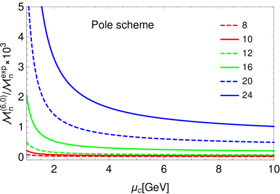
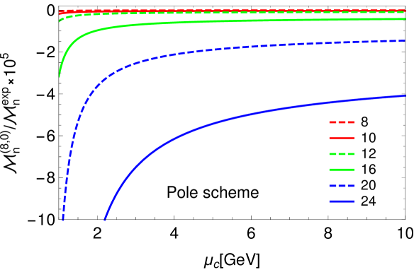
Figure 9: Relative corrections to the non-relativistic moments from the condensate contributions of dimension six (upper panel) and eight (lower panel). The relative corrections have been rescaled by factors of $10^{3}$ and $10^{5}$, respectively.

In Figure 9, the relative contributions of dimension six (upper panel) and eight (lower panel) are shown. Both are significantly smaller than our expectation based on the putative breakdown of the expansion around $n\approx 20$, which would imply that the dimension six and eight corrections are both of the order $1/n\approx 0.05$. This smallness is the result of cancellations between the contribution from the $\Upsilon(1S)$ resonance and the rest that are even stronger than at dimension four. Explicitly, they are at the level of about one part in $3\cdot 10^{5}\,(n=10)$, $5\cdot 10^{4}\,(n=16)$ and $10^{4}\,(n=24)$ at dimension six and about one part in $10^{8}\,(n=10)$, $10^{7}\,(n=16)$ and $2\cdot 10^{6}\,(n=24)$ at dimension eight. We believe that the reason for this behaviour is the off-shellness of the moments which are defined as derivatives of the vacuum polarization function at $q^{2}=0$, far away from the physical cut at $s\geq M_{\Upsilon(1S)}^{2}$. This off-shellness effectively acts as an IR cutoff and suppresses higher-dimensional corrections, which probe the IR regime. On the other hand, the properties of the Upsilon resonances, that we discussed above, are on-shell quantities and the higher-dimensional condensate contributions do not appear suppressed with respect to our expectations from power counting.

From the point of view of the convergence of the condensate expansion, it appears that the moments can be described reliably up to values of $n$ much larger than 20. However, as pointed out in [5], the validity of quark-hadron duality must be questioned when the moment is completely saturated by lowest state. This is the case for the higher values considered here, where the relative contribution of the $\Upsilon(1S)$ to the experimental moments amounts to 95% for $n=20$ and 97% for $n=24$ [5]. By the term ’violation of quark-hadron duality’ we refer to contributions which have a trivial Taylor expansion and are, therefore, not captured by the condensate expansion, like e.g. exponential terms of the form $\text{exp}(-m_{b}/(n\Lambda_{\text{QCD}}))$. Behaviour that is consistent with the presence of such contributions has been observed in the ’t Hooft model [48]. However, the size of these contributions in four-dimensional QCD is difficult to quantify and we do not attempt this here. We note, however, that the exponential terms originate from coherent soft fluctuations [49], e.g. from contributions where the off-shellness is distributed among many soft lines carrying momenta of the order $\Lambda_{\text{QCD}}$, which pushes the bottom pair close to its mass shell. It is conceivable that such an effect does not experience a similar suppression from the effective IR cutoff as the higher-dimensional condensate contributions.

In the range $n\Lambda_{\text{QCD}}\sim m_{b}$ the exponential $\text{exp}(-m_{b}/(n\Lambda_{\text{QCD}}))$ is of order one and we cannot exclude that duality violation effects are relevant at the high accuracy we require for reliable determinations of the bottom-quark mass. We conclude that, in practice, the range of moments is limited by our knowledge of the validity of quark-hadron duality and not by the convergence of the condensate expansion and advise that moments with $n\gtrsim 16$ are not used for determinations of the bottom-quark mass. On the other hand, for $n\approx 10$ duality-violating effects are exponentially suppressed and the condensate expansion provides a reliable determination of the non-perturbative effects. Our results given in Figure 8 and 9 show that the condensate contributions in this region are in the subpercent range and can safely be neglected compared to the perturbative uncertainties.

5 Conclusions

We have determined the leading order condensate corrections to the $\Upsilon(NS)$ masses, leptonic decay rates and sum rules up to and including dimension eight. In addition the potential NLO corrections to the dimension-four contribution have been computed, which allows us to assess the preferred scale choice in the condensate corrections. Our results suggest that the expansion is well behaved for the mass of the $\Upsilon(1S)$, but breaks down for the higher states. The former observation has been used to determine the bottom-quark mass with the results given in (44) and (45).

The leading order condensate corrections to $\Gamma(\Upsilon(1S)\to l^{+}l^{-})$ have a small window of convergence for $0.8\,\text{GeV}\lesssim\mu_{c}\lesssim 1.6\,\text{GeV}$, where they lead to good agreement with the experimental value, but the partial NLO corrections to the dimension-four contribution exceed the leading order correction and cause us to question the perturbative stability. Thus, a final verdict for the leptonic decay rate of the $\Upsilon(1S)$ is only possible once the missing ultrasoft correction has been calculated.

Last but not least, we have considered the non-relativistic moments (53). We find extremely good convergence of the higher-dimensional condensate contributions which clearly shows that non-perturbative contributions to moments with $n\approx 10$ are negligible. On the other hand, we cannot unambiguously exclude the possibility of relevant violations of of quark-hadron duality for $n\gtrsim 16$ despite the surprising smallness of the dimension six and eight corrections. Thus, the non-relativistic moments with $n\approx 10$ remain the theoretically cleanest approach for determinations of the bottom-quark mass from the $\Upsilon$ system.

Acknowledgements

I am grateful to M. Beneke, A. Maier and M. Stahlhofen for helpful discussions, to A. Maier for comments on the manuscript and to V. Mateu and P. Ortega for communication regarding [12]. I wish to thank the Erwin Schrödinger International Institute for Mathematics and Physics (ESI) in Vienna for hospitality during the programme Challenges and Concepts for Field Theory and Applications in the Era of LHC Run-2 where part of this work was done.

Appendix A Condensate corrections to the energy levels and wave functions

We give the results for the condensate corrections to the energy levels and the wave functions at the origin of the S-wave bottomonium states. The contributions are parametrized as

$$E_{N} = E_{N}^{(0)}\left(1+\sum\limits_{i=1}^{\infty}e_{N}^{(i)}+\sum\limits_{k=4,6,8,\dots}\sum\limits_{l=0}^{\infty}e_{N}^{(k,l)}\right),$$ (56)

$$|\psi_{N}(0)|^{2} = |\psi_{N}^{(0)}(0)|^{2}\left(1+\sum\limits_{i=1}^{\infty}f_{N}^{(i)}+\sum\limits_{k=4,6,8,\dots}\sum\limits_{l=0}^{\infty}f_{N}^{(k,l)}\right),$$ (57)

where the leading order expressions are given by

$$E_{n}^{(0)}=-\frac{m_{b}\alpha_{s}^{2}C_{F}^{2}}{4n^{2}},\hskip 42.67912pt|\psi_{n}^{(0)}(0)|^{2}=\frac{1}{\pi}\left(\frac{m_{b}\alpha_{s}C_{F}}{2n}\right)^{3},$$ (58)

the perturbative corrections of relative order $\alpha_{s}^{i}$ are $e_{N}^{(i)}$ and $f_{N}^{(i)}$, and $e_{N}^{(k,l)},f_{N}^{(k,l)}$ are the condensate corrections of relative order $(\Lambda_{\text{QCD}}/(m_{b}\alpha_{s}^{2}))^{k}\alpha_{s}^{l+2}$ to the $N$th energy level and wave function, respectively. At dimension four, we obtain

$$e_{N}^{(4,0)} = R_{4}\,\frac{32N^{6}\left(25515N^{6}-109935N^{4}+101216N^{2}-26624\right)}{6561N^{4}-25920N^{2}+16384},$$ (59)

$$f_{N}^{(4,0)} = -R_{4}\,\frac{32N^{6}}{9\left(6561N^{4}-25920N^{2}+16384\right)^{2}}$$ (60)

$$\times\Big{(}4519905705N^{10}-36791660430N^{8}+101725313184N^{6}$$

$$-112065638400N^{4}+50981371904N^{2}-7583301632\Big{)},$$

in agreement with the results from [24, 25]. For the dimension-six corrections to the energy levels and wave functions, we find

$$e_{N}^{(6,0)} = R_{6}\,\frac{4096N^{10}}{81\left(9N^{2}-64\right)\left(6561N^{4}-25920N^{2}+16384\right)^{3}}$$ (61)

$$\times\big{[}65241222927111N^{16}-1327743092409993N^{14}+10789755579716526N^{12}$$

$$-46158344158975776N^{10}+114216987240880128N^{8}$$

$$-168309372752363520N^{6}+145600287615221760N^{4}$$

$$-68153404341354496N^{2}+13295844358881280\big{]},$$

$$f_{N}^{(6,0)} = R_{6}\,\frac{4096N^{10}}{81(64-9N^{2})^{2}(1024-81N^{2})(6561N^{4}-25920N^{2}+16384)^{4}}$$ (62)

$$\times\big{[}1560233733912305862795N^{24}-68302865242974003997572N^{22}$$

$$+1257835587897041879681466N^{20}-12922847845013954087408448N^{18}$$

$$+82659284132080163141376000N^{16}-347414281805040198547931136N^{14}$$

$$+985563190675064665304727552N^{12}-1906052104684436293825855488N^{10}$$

$$+2504628423489707401549971456N^{8}-2195117868501221112538988544N^{6}$$

$$+1227049495579909701471567872N^{4}-395519535823226068598259712N^{2}$$

$$+55919902706900903797981184\big{]}.$$

The correction to the energy levels is identical to the result of [27]. Our result for the wave function correction however differs from the one in [27] in the coefficients in the square bracket that multiply powers of $N$, while the constant term is in agreement. Numerically the difference is tiny, dropping from 3 permille for $N=1$ to 1.8 permille for $N=10$. Our dimension-eight results read

$$e_{N}^{(8,0)} = R_{8}\,\frac{131072N^{14}}{6561(64-9N^{2})^{3}(1024-81N^{2})(16384-25920N^{2}+6561N^{4})^{5}}$$

$$\times\big{[}513297061199674600970728035N^{30}-28809695301605440114072286106N^{28}$$

$$+714217935339861807140929892403N^{26}-10391224399757404953006517310268N^{24}$$

$$+99331264481676577483010819164416N^{22}-661340018691822569991363819749376N^{20}$$

$$+3169778592264419379462212875714560N^{18}-11139087489514263003228295894401024N^{16}$$

$$+28931645127160026102581319759298560N^{14}-55513215835612849636269917466525696N^{12}$$

$$+78003482654565522219373939233128448N^{10}-78799349232622194122863330417704960N^{8}$$

$$+55418913930949175463048951864754176N^{6}-25648900900141403595678833574936576N^{4}$$

$$+6999998028019916122574328222973952N^{2}-851560509652109050320418236268544\big{]},$$

$$f_{N}^{(8,0)} = R_{8}\,\frac{-131072N^{14}\,(1600-81N^{2})^{-2}(256-9N^{2})^{-1}}{59049(64-9N^{2})^{4}(1024-81N^{2})^{3}(16384-25920N^{2}+6561N^{4})^{6}}$$ (64)

$$\times\big{[}739783191218801346196996467082948404493005N^{46}$$

$$-118424806386048034335763849263957780781041084N^{44}$$

$$+8614327589477425734307468706116579381193741895N^{42}$$

$$-378783092051612274031903244647052432202630343536N^{40}$$

$$+11297942118461809329963818184791182730335090044672N^{38}$$

$$-243143128750125652415373537739611048866722611757056N^{36}$$

$$+3920817963564181189981156819150310468833247662964736N^{34}$$

$$-48564520997046676673717761034578880399807666580357120N^{32}$$

$$+469935568662507411174423052932263135345073787276099584N^{30}$$

$$-3594124289377594431764429130697307804693677753786957824N^{28}$$

$$+21896983904235671174732114490714870006523720168378466304N^{26}$$

$$-106786420612452063591697653002182767135747603942793543680N^{24}$$

$$+417824025967497761694434177318848448549510813159365017600N^{22}$$

$$-1311624595310101793819336380085499993464121204574984863744N^{20}$$

$$+3295683076732204940723945262255632915195793616243217399808N^{18}$$

$$-6596089628312909075581437831841936847452213443718287458304N^{16}$$

$$+10433707912422547412099437180603984258749322917926072745984N^{14}$$

$$-12894168869874165524006895663064691969753810987628940492800N^{12}$$

$$+12244261212399551038854557341492532616026313680323426123776N^{10}$$

$$-8720306429636174559372052451043628307310497364671742345216N^{8}$$

$$+4489452005081410411327292504232625921839722110283767873536N^{6}$$

$$-1572764930888520531444116515121465620114569888243055067136N^{4}$$

$$+334662695930263285190103020209714815173408421809068441600N^{2}$$

$$-32577921122492492137783209690205922464480693174927360000\big{]}.$$

The NLO corrections to the dimension-four condensate contributions have the form

$$e_{N}^{(4,1)} = R_{4}\,\frac{\alpha_{s}}{4\pi}\left[\frac{C_{A}/2-C_{F}}{-C_{F}}\widetilde{e}_{N}^{\text{ DVD}}+\widetilde{e}_{N}^{\text{ DDV}}+\widetilde{e}_{N}^{\text{ us}}\right],$$ (65)

$$f_{N}^{(4,1)} = R_{4}\,\frac{\alpha_{s}}{4\pi}\left[\frac{C_{A}/2-C_{F}}{-C_{F}}\widetilde{f}_{N}^{\text{ DVD}}+\widetilde{f}_{N}^{\text{ DDV}}+\widetilde{f}_{N}^{\text{ us}}\right],$$ (66)

where the potential terms are

$$\widetilde{e},_{N}^{\text{ DVD}} = \frac{128N^{6}}{9\left(6561N^{4}-25920N^{2}+16384\right)^{2}}\Bigg{\{}2\left[a_{1}+2\beta_{0}\left(S_{1}+L_{N}\right)\right]\Big{(}167403915N^{10}$$ (67)

$$-1486558575N^{8}+4690934208N^{6}-6303780864N^{4}+3483631616N^{2}$$

$$-536870912\Big{)}+\beta_{0}(9N-8)\Big{(}94419351N^{9}+46727442N^{8}-800382951N^{7}$$

$$-381105162N^{6}+2367378684N^{5}+1061906784N^{4}-2883647232N^{3}$$

$$-1162401792N^{2}+1320550400N+405274624\Big{)}\Bigg{\}},$$

$$\widetilde{e},_{N}^{\text{ DDV}} = \left[a_{1}+2\beta_{0}\left(S_{1}+L_{N}\right)\right]\frac{-32N^{6}}{9\left(6561N^{4}-25920N^{2}+16384\right)^{2}}\Big{(}5859137025N^{10}$$ (68)

$$-48288205485N^{8}+136847786688N^{6}-159273676800N^{4}$$

$$+81059381248N^{2}-15166603264\Big{)}+$$

$$\beta_{0}\frac{32N^{6}}{3\left(6561N^{4}-25920N^{2}+16384\right)}\Big{(}451332N^{6}-161595N^{5}-1797839N^{4}$$

$$+646725N^{3}+1160272N^{2}-425280N+7168\Big{)},$$

$$\widetilde{f},_{N}^{\text{ DVD}} = \left(a_{1}+2\beta_{0}L_{N}\right)\frac{256N^{6}}{81\left(6561N^{4}-25920N^{2}+16384\right)^{3}}\Big{(}-29655101330505N^{14}$$ (69)

$$+370819521046350N^{12}-1836925493383872N^{10}+4598115283537920N^{8}$$

$$-6194386829574144N^{6}+4467901285269504N^{4}-1563638678683648N^{2}$$

$$+189115999977472\Big{)}+\beta_{0}\frac{128N^{5}}{81\left(6561N^{4}-25920N^{2}+16384\right)^{2}}\Bigg{\{}$$

$$\frac{1}{9\left(6561N^{4}-25920N^{2}+16384\right)^{2}}\Big{(}-8888937845922281277N^{19}$$

$$+2334805437953319660N^{18}+146679930871209367335N^{17}$$

$$-38038386654486402750N^{16}-1019696917323083770998N^{15}$$

$$+260020266583548188160N^{14}+3893749911649043582976N^{13}$$

$$-970389752080885235712N^{12}-8954749600639565709312N^{11}$$

$$+2161122845010608259072N^{10}+12847315095944310030336N^{9}$$

$$-2955869597186629042176N^{8}-11551005743863723720704N^{7}$$

$$+2436883078824792686592N^{6}+6290577008666263683072N^{5}$$

$$-1065043454471757103104N^{4}-1829313053453482721280N^{3}$$

$$+131764347572768997376N^{2}+182269121168985292800N$$

$$+36893488147419103232\Big{)}+\frac{36NS_{1}}{6561N^{4}-25920N^{2}+16384}$$

$$\times\Big{(}-3295011258945N^{14}+41202169005150N^{12}-204102832598208N^{10}$$

$$+510901698170880N^{8}-688295779762176N^{6}+498462848188416N^{4}$$

$$-178391466639360N^{2}+21990232555520\Big{)}-\frac{33554432N}{6561N^{4}-25920N^{2}+16384}$$

$$\times\Bigg{[}\left(-32805N^{6}+2177280N^{4}-4993024N^{2}+1048576\right)S_{1}\left(\frac{N}{8}\right)$$

$$+\left(-111537N^{6}+124416N^{4}-5386240N^{2}+7340032\right)S_{1}\left(\frac{9N}{8}\right)\Bigg{]}$$

$$-36N^{2}\left(S_{2}-\frac{\pi^{2}}{6}\right)\Big{(}-167403915N^{10}+1486558575N^{8}-4690934208N^{6}$$

$$+6303780864N^{4}-3483631616N^{2}+536870912\Big{)}\Bigg{\}},$$

$$\widetilde{f},_{N}^{\text{ DDV}} = \left(a_{1}+2\beta_{0}L_{N}\right)\frac{-64N^{6}}{81\left(6561N^{4}-25920N^{2}+16384\right)^{3}}\Big{(}-385516317296565N^{14}$$ (70)

$$+4654961778867030N^{12}-21965572921731408N^{10}+51360436390947840N^{8}$$

$$-63132424989769728N^{6}+41064256744980480N^{4}-13147993330941952N^{2}$$

$$+1582746988183552\Big{)}-\beta_{0}\frac{32N^{5}}{81\left(6561N^{4}-25920N^{2}+16384\right)^{2}}\Big{\{}$$

$$\frac{1}{9\left(6561N^{4}-25920N^{2}+16384\right)^{2}}\Big{(}61405383018172307058N^{19}$$

$$-22180651660556536770N^{18}-965837565458451500139N^{17}$$

$$+351080411169493108575N^{16}+6289521884171512783128N^{15}$$

$$-2307675798943664843520N^{14}-21902675740289714221056N^{13}$$

$$+8153996687233488691200N^{12}+44045654765398681780224N^{11}$$

$$-16799371281675894915072N^{10}-51685121285332515422208N^{9}$$

$$+20621242559717072437248N^{8}+33974735719419655225344N^{7}$$

$$-14944437608241652826112N^{6}-10679923278040006656000N^{5}$$

$$+6036677324559894970368N^{4}+609631074176867500032N^{3}$$

$$-1054643390588414590976N^{2}+220638101144321654784N$$

$$-18446744073709551616\Big{)}+\frac{4NS_{1}}{6561N^{4}-25920N^{2}+16384}$$

$$\times\Big{(}-652412229271110N^{14}+7881876138460500N^{12}-37221596700680304N^{10}$$

$$+87133432412759040N^{8}-107286357009825792N^{6}+69985956437950464N^{4}$$

$$-22538834096947200N^{2}+2696552267120640\Big{)}+\frac{16777216N}{6561N^{4}-25920N^{2}+16384}$$

$$\Big{(}\left(203391N^{6}-13405824N^{4}+24866816N^{2}+1048576\right)S_{1}\left(\frac{N}{8}\right)$$

$$+\left(-465831N^{6}+30824064N^{4}-64811008N^{2}+7340032\right)S_{1}\left(\frac{9N}{8}\right)\Big{)}$$

$$-18N^{2}\left(S_{2}-\frac{\pi^{2}}{6}\right)\Big{(}-5859137025N^{10}+48288205485N^{8}-136847786688N^{6}$$

$$+159273676800N^{4}-81050992640N^{2}+14629732352\Big{)}\Bigg{\}},$$

where $L_{N}=\ln(N\mu/(m\alpha_{s}C_{F}))$, $S_{1}(x)=\sum_{k=1}^{x}k^{-1}$ is the analytic continuation of the harmonic number to non-integer values and $S_{i}=\sum_{k=1}^{N}k^{-i}$ without an explicit argument is the $N$th harmonic number of rank $i$. The ultrasoft corrections $\widetilde{e}_{N}^{\text{ us}}$ and $\widetilde{f}_{N}^{\text{ us}}$ are currently unknown.

References

• [1] Y. Kiyo and Y. Sumino, Full Formula for Heavy Quarkonium Energy Levels at Next-to-next-to-next-to-leading Order, Nucl. Phys. B 889 (2014) 156 [arXiv:1408.5590 [hep-ph]].
• [2] Y. Kiyo and Y. Sumino, Perturbative heavy quarkonium spectrum at next-to-next-to-next-to-leading order, Phys. Lett. B 730 (2014) 76 [arXiv:1309.6571 [hep-ph]].
• [3] C. Peset, A. Pineda and M. Stahlhofen, Potential NRQCD for unequal masses and the Bc spectrum at N3LO, JHEP 1605 (2016) 017 [arXiv:1511.08210 [hep-ph]].
• [4] M. Beneke, Y. Kiyo, P. Marquard, A. Penin, J. Piclum, D. Seidel and M. Steinhauser, Leptonic decay of the $\Upsilon$(1$S$) meson at third order in QCD, Phys. Rev. Lett.  112 (2014) no.15, 151801 [arXiv:1401.3005 [hep-ph]].
• [5] M. Beneke, A. Maier, J. Piclum and T. Rauh, The bottom-quark mass from non-relativistic sum rules at NNNLO, Nucl. Phys. B 891 (2015) 42 [arXiv:1411.3132 [hep-ph]].
• [6] M. Beneke, A. Maier, J. Piclum and T. Rauh, NNNLO determination of the bottom-quark mass from non-relativistic sum rules, PoS RADCOR 2015 (2016) 035 [arXiv:1601.02949 [hep-ph]].
• [7] A. A. Penin and N. Zerf, Bottom Quark Mass from $\Upsilon$ Sum Rules to ${\cal O}(\alpha_{s}^{3})$, JHEP 1404 (2014) 120 [arXiv:1401.7035 [hep-ph]].
• [8] A. Hoang, P. Ruiz-Femenía and M. Stahlhofen, Renormalization Group Improved Bottom Mass from Upsilon Sum Rules at NNLL Order, JHEP 1210 (2012) 188 [arXiv:1209.0450 [hep-ph]].
• [9] C. Ayala, G. Cvetič and A. Pineda, The bottom quark mass from the $\bm{\Upsilon}(1S)$ system at NNNLO, JHEP 1409 (2014) 045 [arXiv:1407.2128 [hep-ph]].
• [10] C. Ayala, G. Cvetič and A. Pineda, Mass of the bottom quark from Upsilon(1S) at NNNLO: an update, J. Phys. Conf. Ser.  762 (2016) no.1, 012063 [arXiv:1606.01741 [hep-ph]].
• [11] Y. Kiyo, G. Mishima and Y. Sumino, Determination of mc and mb from quarkonium 1S energy levels in perturbative QCD, Phys. Lett. B 752 (2016) 122 Erratum: [Phys. Lett. B 772 (2017) 878] [arXiv:1510.07072 [hep-ph]].
• [12] V. Mateu and P. G. Ortega, Bottom and Charm Mass determinations from global fits to $Q\bar{Q}$ bound states at N3LO, arXiv:1711.05755 [hep-ph].
• [13] A. Pineda and J. Soto, Effective field theory for ultrasoft momenta in NRQCD and NRQED, Nucl. Phys. Proc. Suppl.  64 (1998) 428 [hep-ph/9707481].
• [14] M. Beneke, A. Signer and V. A. Smirnov, Top quark production near threshold and the top quark mass, Phys. Lett. B 454 (1999) 137 [hep-ph/9903260].
• [15] N. Brambilla, A. Pineda, J. Soto and A. Vairo, Potential NRQCD: An Effective theory for heavy quarkonium, Nucl. Phys. B 566 (2000) 275 [hep-ph/9907240].
• [16] M. Beneke, Y. Kiyo and K. Schuller, Third-order correction to top-quark pair production near threshold I. Effective theory set-up and matching coefficients, arXiv:1312.4791 [hep-ph].
• [17] M. Beneke, Perturbative heavy quark - anti-quark systems, PoS hf 8 (1999) 009 [hep-ph/9911490].
• [18] R. N. Lee, A. V. Smirnov, V. A. Smirnov and M. Steinhauser, Analytic three-loop static potential, Phys. Rev. D 94 (2016) no.5, 054029 [arXiv:1608.02603 [hep-ph]].
• [19] M. Beneke, Y. Kiyo, P. Marquard, A. Penin, J. Piclum and M. Steinhauser, Next-to-Next-to-Next-to-Leading Order QCD Prediction for the Top Antitop $S$-Wave Pair Production Cross Section Near Threshold in $e^{+}e^{-}$ Annihilation, Phys. Rev. Lett.  115 (2015) no.19, 192001 [arXiv:1506.06864 [hep-ph]].
• [20] M. Beneke, A. Maier, T. Rauh and P. Ruiz-Femenía, Non-resonant and electroweak NNLO correction to the $e^{+}e^{-}$ top anti-top threshold, JHEP 1802 (2018) 125 [arXiv:1711.10429 [hep-ph]].
• [21] I. I. Y. Bigi, Y. L. Dokshitzer, V. A. Khoze, J. H. Kühn and P. M. Zerwas, Production and Decay Properties of Ultraheavy Quarks, Phys. Lett. B 181 (1986) 157.
• [22] V. S. Fadin and V. A. Khoze, Threshold Behavior of Heavy Top Production in $e^{+}e^{-}$ Collisions, JETP Lett.  46 (1987) 525 [Pisma Zh. Eksp. Teor. Fiz.  46 (1987) 417].
• [23] M. B. Voloshin, On Dynamics of Heavy Quarks in Nonperturbative QCD Vacuum, Nucl. Phys. B 154 (1979) 365.
• [24] M. B. Voloshin, Precoulombic Asymptotics for Energy Levels of Heavy Quarkonium, Sov. J. Nucl. Phys.  36 (1982) 143 [Yad. Fiz.  36 (1982) 247].
• [25] H. Leutwyler, How to Use Heavy Quarks to Probe the QCD Vacuum, Phys. Lett.  98B (1981) 447.
• [26] M. B. Voloshin, Precision determination of $\alpha_{s}$ and $m_{b}$ from QCD sum rules for $b\bar{b}$, Int. J. Mod. Phys. A 10 (1995) 2865 [hep-ph/9502224].
• [27] A. Pineda, Next-to-leading nonperturbative calculation in heavy quarkonium, Nucl. Phys. B 494 (1997) 213 [hep-ph/9611388].
• [28] E. Wichmann and C. Woo, Integral Representation for the Nonrelativistic Coulomb Green’s Function, J. Math. Ph. 2 (1961) 178.
• [29] M. B. Voloshin, Nonperturbative Effects In Hadronic Annihilation Of Heavy Quarkonium, Sov. J. Nucl. Phys.  40 (1984) 662 [Yad. Fiz.  40 (1984) 1039].
• [30] M. Beneke, Y. Kiyo and K. Schuller, Third-order correction to top-quark pair production near threshold II. Potential contributions, in preparation.
• [31] M. Beneke, J. Piclum and T. Rauh, P-wave contribution to third-order top-quark pair production near threshold, Nucl. Phys. B 880 (2014) 414 [arXiv:1312.4792 [hep-ph]].
• [32] M. Beneke, P. Falgari and C. Schwinn, Threshold resummation for pair production of coloured heavy (s)particles at hadron colliders, Nucl. Phys. B 842 (2011) 414 [arXiv:1007.5414 [hep-ph]].
• [33] N. Brambilla, X. Garcia i Tormo, J. Soto and A. Vairo, The Logarithmic contribution to the QCD static energy at N4LO, Phys. Lett. B 647 (2007) 185 [hep-ph/0610143].
• [34] N. Brambilla, D. Gromes and A. Vairo, Poincare invariance constraints on NRQCD and potential NRQCD, Phys. Lett. B 576 (2003) 314 [hep-ph/0306107].
• [35] M. A. Shifman, A. I. Vainshtein and V. I. Zakharov, QCD and Resonance Physics: Applications, Nucl. Phys. B 147 (1979) 448.
• [36] G. S. Bali, C. Bauer and A. Pineda, Model-independent determination of the gluon condensate in four-dimensional SU(3) gauge theory, Phys. Rev. Lett.  113 (2014) 092001 [arXiv:1403.6477 [hep-ph]].
• [37] C. A. Dominguez, L. A. Hernandez and K. Schilcher, Determination of the gluon condensate from data in the charm-quark region, JHEP 1507 (2015) 110 [arXiv:1411.4500 [hep-ph]].
• [38] M. Beneke, Y. Kiyo, A. Maier and J. Piclum, Near-threshold production of heavy quarks with QQbar_threshold, Comput. Phys. Commun.  209 (2016) 96 [arXiv:1605.03010 [hep-ph]].
• [39] M. Beneke, A Quark mass definition adequate for threshold problems, Phys. Lett. B 434 (1998) 115 [hep-ph/9804241].
• [40] K. G. Chetyrkin, J. H. Kühn, A. Maier, P. Maierhofer, P. Marquard, M. Steinhauser and C. Sturm, Charm and Bottom Quark Masses: An Update, Phys. Rev. D 80 (2009) 074010 [arXiv:0907.2110 [hep-ph]].
• [41] K. G. Chetyrkin, J. H. Kühn, A. Maier, P. Maierhofer, P. Marquard, M. Steinhauser and C. Sturm, Addendum to ”Charm and Bottom Quark Masses: An Update”, Phys. Rev. D 96 (2017) 116007 [arXiv:1710.04249 [hep-ph]].
• [42] P. Marquard, A. V. Smirnov, V. A. Smirnov and M. Steinhauser, Quark Mass Relations to Four-Loop Order in Perturbative QCD, Phys. Rev. Lett.  114 (2015) no.14, 142002 [arXiv:1502.01030 [hep-ph]].
• [43] P. Marquard, A. V. Smirnov, V. A. Smirnov, M. Steinhauser and D. Wellmann, $\overline{\rm MS}$-on-shell quark mass relation up to four loops in QCD and a general SU$(N)$ gauge group, Phys. Rev. D 94 (2016) no.7, 074025 [arXiv:1606.06754 [hep-ph]].
• [44] A. Pineda, Determination of the bottom quark mass from the $\Upsilon(1S)$ system, JHEP 0106 (2001) 022 [hep-ph/0105008].
• [45] N. Brambilla, A. Pineda, J. Soto and A. Vairo, Effective field theories for heavy quarkonium, Rev. Mod. Phys.  77 (2005) 1423 [hep-ph/0410047].
• [46] D. J. Broadhurst, P. A. Baikov, V. A. Ilyin, J. Fleischer, O. V. Tarasov and V. A. Smirnov, Two loop gluon condensate contributions to heavy quark current correlators: Exact results and approximations, Phys. Lett. B 329 (1994) 103 [hep-ph/9403274].
• [47] K. Chetyrkin, J. H. Kühn, A. Maier, P. Maierhofer, P. Marquard, M. Steinhauser and C. Sturm, Precise Charm- and Bottom-Quark Masses: Theoretical and Experimental Uncertainties, Theor. Math. Phys.  170 (2012) 217 [arXiv:1010.6157 [hep-ph]].
• [48] I. I. Y. Bigi, M. A. Shifman, N. Uraltsev and A. I. Vainshtein, Heavy flavor decays, OPE and duality in two-dimensional ’t Hooft model, Phys. Rev. D 59 (1999) 054011 [hep-ph/9805241].
• [49] M. A. Shifman, Quark hadron duality, hep-ph/0009131.