Deep JVLA Imaging of GOODS-N at 20cm

Abstract

New wideband continuum observations in the $1-2$ GHz band of the GOODS-N field using NSF’s Karl G. Jansky Very Large Array (VLA) are presented. The best image with an effective frequency of 1525 MHz reaches an rms noise in the field center of $2.2\mu$Jy with $1.6$^′′ resolution. A catalog of 795 sources is presented covering a radius of nine arcminutes centered near the nominal center for the GOODS-N field, very near the nominal VLA pointing center for the observations. Optical/NIR identifications and redshift estimates both from ground-based and HST observations are discussed. Using these optical/NIR data, it is most likely that fewer than 2% of the sources without confusion problems do not have a correct identification. A large subset of the detected sources have radio sizes $>1$^′′. It is shown that the radio orientations for such sources correlate well with the HST source orientations especially for $z<1$. This suggests that a least a large subset of the 10kpc-scale disks of LIRG/ULIRG galaxies have strong star-formation, not just in the nucleus. For the half of the objects with $z>1$, the sample must be some mixture of very high star-formation rates, typically 300 M$\odot$/yr assuming pure star-formation, and an AGN or a mixed AGN/star-formation population.

1 Introduction

Deep radio continuum surveys combined with data from other wavelength bands can shed new light on the nature of galaxy evolution. Both AGN and star-forming galaxies produce synchrotron emission which can be detected at centimeter wavelengths. The radio results can be compared with deep surveys in other bands to determine which processes are most important for a given object. Furthermore the surface brightness distribution in the radio can shed light on the detailed physics. AGN activity is usually associated with jets, lobes, and/or extremely compact, usually self-absorbed emission. Star-formation always has brightness temperatures $<10^{5}K$ and can either be due to a relatively compact nuclear star-burst or much larger star-formation distributed within a galaxy’s disk [Condon, 1992]. Synchrotron emission more extended than an individual galaxy can also be associated with an ongoing galaxy-galaxy merger [e.g. Condon, Helou, & Jarrett, 2002, Chyzy & Beck, 2004]. Very extended emission can also be associated with galaxy winds, often along the minor axis of a galaxy, as in the local system M82 [Seaquist & Odegard, 1991, Adebhar et al., 2013]. Evidence for powerful galactic winds is known from optical line emission [e.g. Martin et al., 2012] and we might well expect to see low surface brightness analogs in the radio band. Finally, AGN are known to blow bubbles in local cooling cores, which are evidence of feedback which suppresses cooling [e.g. Owen, Eilek & Kassim, 2000, Pfrommer, 2013]. At higher redshifts, such core-halo radio emission or radio emission associated with other AGN tracers would be consistent with such phenomena and would be important to understanding the role of AGN feedback in galaxy evolution.

However, deep radio surveys with arcsecond scale resolution with current radio arrays are only just able to detect radio surface brightness which allows the detection of such extended structures Low S/N means that when we detect such structures very little detail will be revealed. Thus we need to survey regions of the sky which have been well studied at other wavelengths to give us clues as to what we are observing.

GOODS-N [Dickinson et al., 2003] is one of a few very well studied extragalactic survey regions in the sky. It contains the original Hubble deep field [Williams et al., 1996] and has been expanded to include the best or near-best ancillary data in every wavelength region. The field was originally observed at 1.4 GHz with the VLA in 1996 [Richards, 2000] and those data were combined with Merlin imaging to produce a higher resolution image of a smaller field [Muxlow et al., 2005]. The VLA survey was most recently improved by Morrison et al. [2010] who increased the total integration time to 165 hours. For VLA observations the GOODS-N high declination (62°) is ideal for deep imaging since it can be observed above 20° for 15 hours and the uv-tracks are almost circular producing very good imaging. However, some bright confusing radio sources well outside the GOODS-N field itself have limited previous images to noise levels worse than theoretical. The upgraded JVLA now allows much wider bandwidths to be observed simultaneously (1-2 GHz in the L-band) than the old VLA surveys which typically used a total bandwidth of 44 MHz at 1.4 GHz (20cm). Besides improving the sensitivity per unit time, the wider bandwidths produce more complete uv-coverage and thus a better synthesized beam. This better beam reduces the impact of the confusing sources on imaging and allows a deeper survey. Other systematics which affected the earlier imaging are also less of a problem, i.e. the image-plane smearing due to the integration time and the channel bandwidth. The overall effect of the new VLA hardware is to produce a superior image with fewer systematics and less drop-off in sensitivity with distance from the field center.

Several papers [Barger et al., 2012, Tan et al., 2013, Rudnick & Owen, 2014, Barger et al., 2014, Tan et al., 2014, To, Wang & Owen, 2014, Barger et al., 2015, 2017, Cowie et al., 2017, Lui et al., 2017] have made use of the data reported here and this paper provides the long promised documentation for the survey as well as the catalog of the sources with peak flux densities above $5\sigma$. The discussion is also intended to put the survey in perspective for future studies, as well as discussing some of the properties of the extended sources and their optical identifications.

2 Observations and Reductions

The GOODS-N field was observed in the A-configuration for a total of 39 hours including calibration and move time between August 9 and September 11, 2011. A single field was observed, centered at 12 $\!\!{}^{\mathrm{h}}$36 $\!\!{}^{\mathrm{m}}$49.4 $\!\!{}^{\mathrm{s}}$, 62°12^′58^′′ . Eight different scheduling blocks were observed, each of 5 hours, except for one which was 4 hours long. Roughly 33 hours of this time were spent on-source. The observations covered the bands from $1000-1512$ and $1520-2032$ MHz using 1 MHz channels. A phase, bandpass and instrumental polarization calibrator, J1313+6735, was observed every twenty minutes. 3C286 was observed to calibrate the flux density scale and the polarization position angles.

For each scheduling block, the data were edited and calibrated in AIPS in the standard way. The worst parts of the band, in particular between 1520 and 1648 MHz, were flagged at the beginning of this process. Also about 12% of the data were flagged due to subband edge effects in the JVLA WIDAR correlator. The rest of the dataset was edited using the RFLAG task, resulting in a few percent more of the total being removed. The data were generally well-behaved and required no unusual editing. A delay correction was calculated using the task FRING. The bandpass was then calculated without any calibration except for the delay correction. After total intensity calibration, the uv-data weights were calibrated using the AIPS task, REWAY. REWAY tends to produce lower weights in regions with more interference and near the edges of the 1000-2000 GHz band, where the system is less sensitive. Details of the polarization calibration and results are discussed in Rudnick & Owen [2014].

3 Imaging and Self-calibration

Narrow band images were first made with one five hour track. These images were used as a model for self-calibration of all the subbands. The flux density calibration for each subband was held fixed for each track/subband during self calibration. The task EDITA was further used to edit out uv-data which had large discrepant solutions. In practice $<1$% of the data were edited out as a result of this step. The whole process was repeated until all the solutions converged with small errors. The uv-data were then merged and optimally averaged for each subband/baseline to minimize the size of the dataset to be imaged without distorting the image, using the AIPS procedure, STUFFR. The uv-data were then ported to CASA.

The total intensity data were imaged in CASA using the clean task. In particular, wide-field, nterms=2, and Briggs weighting with robust=0.5 were used. For these parameters, the Multi-Scale-Multi-Frequency-Synthesis algorithm was used [Rau & Cornwell, 2011]. This imaging algorithm solves for the total intensity and spectral index image across the full bandwidth, in this case 1-2 GHz. The W-projection was also used which corrects for the three dimensional sky curvature. The scales used in the imaging were 0.35^′′$\times(0,3,10)$, where 0.35^′′ was the pixel size used in clean. For detailed testing of this algorithm and comparison to other imaging approaches see Rau, Bhatnagar & Owen [2016] and references therein. After imaging the CASA task widebandpbcor was used to correct for the primary beam attenuation. This combination of parameters produced an image with 1.6^′′ resolution and a rms noise of $2.2\mu$Jy, before the primary beam correction. The usually assumed parameters in the VLA Exposure Calculator for 33 hours on-source, robust weighting and 600MHz bandwidth yield an expected rms of $1.9\mu$Jy.

4 Analysis Region

The single pointing center for these VLA observations was 12 $\!\!{}^{\mathrm{h}}$36 $\!\!{}^{\mathrm{m}}$49.4 $\!\!{}^{\mathrm{s}}$, 62°12^′58^′′ (J2000.0), the same as used by Richards [2000] and Morrison et al. [2010]. As such the imaging covers a region almost 1° on each side and has useful results out to at least 20^′ from the pointing center. However, this paper is focused on the GOODS-N area and the analysis is only of a region of the image 9^′ in radius, centered on 12 $\!\!{}^{\mathrm{h}}$36 $\!\!{}^{\mathrm{m}}$55.10 $\!\!{}^{\mathrm{s}}$, 62°14^′15^′′ , which contains all the original GOODS-N HST fields. Thus the field chosen for analysis is about 1.5^′ from the pointing center and contains some sources just outside the GOODS-N region. Besides limiting the analysis to the regions studied most intensely at all wavelengths, the 9^′ radius, centered very close to the pointing center, limits the study to the most sensitive part of the VLA primary beam, where the smallest instrumental corrections are required. In figure 1, we show the 1.6^′′ resolution image and the 9^′ survey region for reference.

Figure 1: Grey Scale 1.6^′′  GOODS-N radio image. 1.6^′′$\times$1.6^′′ clean beam is shown as a very small blue dot in lower left corner of the image. The red circle is the 9^′ radius limit of the catalog. The grey scale wedge on the top of the image shows the range of intensities displayed from $-5\mu$Jy to $20\mu$Jy.

5 Results

5.1 The Catalog

5.1.1 Catalog Construction

The catalog was constructed using the AIPS image cataloging task, SAD. However, SAD, like other such cataloging tools, is best at finding and cataloging sources with sizes near the resolution of the image the task is given to analyze. If one wants to catalog sources with a wider range of sizes something more should be done.

Our final images were analyzed in several different ways in order to assemble the most complete list of sources. The main complication is the fact that a significant fraction of the sources are resolved. The most useful source cataloging algorithms involve fitting two dimensional Gaussians to the significant “islands” of emission in the image. That is a good technique as long as the sources are only slightly resolved. When the true angular size of a source is bigger than about one clean restoring beam in size, the assumption of a Gaussian for the shape of the source in the image becomes less than optimum. If a source is very much larger than the clean beam, many Gaussians may be necessary to describe the emission, which are not useful for cataloging and identifying individual sources. If a source is bigger than the clean beam, then peak brightness may fall below the noise cutoff and/or the fit may also not be optimum.

In order to deal with this situation, the final radio image was convolved to several different, lower resolutions. The fitting was done on each image and the results compared. Then the best fit for each source was picked usually based on the resulting signal-to-noise ratio (SNR). When a lower resolution image revealed a significantly higher total flux density that fit was picked. Also if the fit to a higher resolution image with a similar but slightly lower SNR more clearly showed that a source was significantly resolved, then that fit was chosen. Finally, for the sources which were very resolved in all the images, the AIPS task TVSTAT, was used to estimate the total flux density. In this case, the flux density errors were based on the total two dimensional size, and the total size was estimated by hand, i.e. by measuring X,Y positions of the source edges on the AIPS TV display.

The AIPS task SAD was used to create the first version of the source list at each resolution. Images with circular clean beams were calculated from the full resolution image with sizes of 1.6^′′, 2.0^′′, 3.0^′′, 6.0^′′, and 12.0^′′, using the task CONVL. For analysis of sources with peak flux densities $>40\mu$Jy, an extra, higher resolution image was made using robust=0 weighting in CASA clean. This produced an image with a clean beam of 1.02^′′$\times$0.82^′′ at PA=82.75. When this image produced the best fit, it is called “1.0” in the output table. For each of these images, an image of the local rms noise was calculated using the RMSD and these images were used as input to SAD. Each image was search down to peaks of $4.5\times$ the local rms, i.e. $4.5\sigma$. A collated source list from these fits was then fitted by hand using JMFIT, which uses the same Gaussian fitting algorithm as SAD.

For the final fits sources were considered to be resolved if the total fitted flux density exceeded the fitted peak by more than the estimated $1\sigma$ error in the total and the minimum deconvolved, fitted size of the major axis was $>0$. The best fit in peak $\sigma$’s was then chosen above $5\sigma$ for each source. If the source was resolved at one or more resolutions, the best fit from JMFIT or SAD which produced an estimate of the minimum source size $>0$ was chosen. Note that our approach to identifying a resolved source is different from the $2\sigma$ criterion described by Vernstrom et al. [2016], which seems too restrictive based on our results. Perhaps this is because the fits are to Gaussians in both our study and Vernstrom et al. [2016] and the sources are generally not well described as Gaussians if they have sizes in a cleaned image much larger than a clean beam. In any case, the radio-optical alignment results described later in this paper appear to confirm the validity of our method.

Table 1: GOODS-N Radio Source Catalog

Name	RA	err	Dec	err	Pk	err	Tot	err	S/N	$<$	Ma	Mi	PA	Res	za
	2000.0	s	2000.0	′′	$\mu$J/b		$\mu$Jy				′′	′′	°	′′
(1)	(2)	(3)	(4)	(5)	(6)	(7)	(8)	(9)	(10)	(11)	(12)	(13)	(14)	(15)	(16)
J123627.5+621026	12 36 27.53	0.02	62 10 26.1	0.1	17.4	2.6	17.4	2.7	6.7	$<$	1.2			1.6	0.761sB
J123627.5+621218	12 36 27.56	0.02	62 12 18.0	0.1	17.1	2.5	17.1	2.6	6.7	$<$	1.4			1.6	noz
J123627.7+621158	12 36 27.78	0.01	62 11 58.6	0.1	22.8	2.6	22.8	2.7	8.9	$<$	1.2			1.6	3.388sH
J123628.4+622052	12 36 28.44	0.02	62 20 52.9	0.2	15.4	3.1	15.4	3.1	5.0	$<$	0.8			1.6	1.307pQ
J123628.6+622139	12 36 28.67	0.01	62 21 39.7	0.1	37.3	3.2	37.3	3.4	11.5	$<$	1.2			1.6	1.871pQ
J123628.9+620615	12 36 28.97	0.01	62 06 15.9	0.1	45.2	2.9	57.5	6.1	15.5		1.5	0.5	90	2.0	1.264sB
J123629.0+621045	12 36 29.04	0.01	62 10 45.6	0.1	72.6	3.2	91.1	7.1	22.7		2.2	0.5	75	3.0	1.013sB
J123629.3+621613	12 36 29.36	0.08	62 16 13.9	0.5	41.6	6.2	59.3	13.9	9.0		5.0	2.6	98	6.0	0.848sB
J123629.3+621936	12 36 29.36	0.02	62 19 36.3	0.2	17.4	2.9	17.4	2.9	6.0	$<$	1.6			1.6	1.005sB
J123629.4+621513	12 36 29.45	0.02	62 15 13.2	0.2	14.2	2.5	14.2	2.5	5.6	$<$	1.8			1.6	3.652sB

In JMFIT and SAD the minimum and maximum values were obtained by deconvolving the source beam parameters with all 27 combinations of the AIPS adverb EFACTOR$\times(-1,0,1)\times$ the uncertainties in the major axis, minor axis, and position angle determined from the fit added to the nominal beam size. Then the maximum and minimum values of the deconvolved sizes and position angle were adopted as the fitted limits on the source size. In order to determine the best value of EFACTOR, 10,000 sources whose peak had a range of SNR from 4 to 50 and which were either points or one arcsecond FWHM Gaussians were convolved with the clean beam of the 1.6^′′ resolution image and added to random points near the center of that image of the 1.6^′′ resolution image. A range of values for EFACTOR were then tried for the fit to each source in order to minimize the number of falsely resolved sources and minimize the number of one arcsecond sources which were found to be resolved. EFACTOR$=1.3$ produced the best overall results. For example for S/N$=5.0$ with EFACTOR$=1.3$, 2.5% of source point sources were found to be resolved and 24% of the one arcsecond Gaussians were classified as resolved with essentially all of the remaining sources given upper size limits $>1$^′′.

5.1.2 Catalog Content

A total of 795 radio sources with a $S/N=5$ or greater in at least one of the images were cataloged using the procedures discussed above. In table 1, we show the first ten lines of the full online table listing the parameters of those sources. Column 1 contains the J2000 source name. In columns $2-5$ we give the J2000 RA, the J2000 Declination and the estimated errors. Columns 6 and 7 contain the peak flux density and the associated error. Columns 8 and 9 list the best estimate of the total flux density and its error. If the total fitted flux density is more than one sigma greater than the peak and the lower limit to the major axis size is greater than 0.0, the total fitted flux density is quoted. Otherwise, the source is assumed to be best represented by a point source and peak flux density and error are quoted here. A 3% scale error has been added in quadrature to account for errors in the flux density calibration and the primary beam correction. In column 10, we give the SNR of the peak detection. If the source is approximated as a point, there is a $<$ sign in column 11 and the associated upper limit is given in column 12. If the source is resolved then columns 12,13 and 14 give the best estimate of the true source size after correcting for the clean beam. Column 15 gives the clean beam size for the image used for the quoted fit. In column 16 we list the redshift. After the numeric redshift, the first letter indicates whether the redshift is spectroscopic (s) or photometric (p). The letters after that indicate the reference for the redshift, as detailed in the table footnotes.

Note that part of J123538.5+621643 is in the nine arcminute field of this survey but not the parent galaxy and thus this source is not included in the catalog (see fig 1).

5.2 Identifications

5.2.1 NIR Identifications

One way to understand the reliability of the catalog is to study the identifications at other bands. Of course, such studies also are necessary to understand the nature of the radio sources. For this purpose the largest number of identifications are found in deep NIR catalogs since deep optical catalogs produce fewer identifications and are more confused by background sources [e.g. Strazzullo et al., 2010, Pannella et al., 2015, Vernstrom et al., 2016]. This is likely because the optical bands are biased against dusty objects and/or the objects have $z\mathrel{\raise 1.50696pt\hbox{$\scriptstyle>$}\kern-6.00006pt\lower 1.72218pt\hbox{{$\scriptstyle\sim$}}}1$, since standard optical bands are redshifted below the 4000Å break. Also the SEDs of the old stellar population stars slowly rise as one follows them from the red rest-frame optical bands into the NIR. We have used the deep Ks catalog of Wang et al. [2010] as our primary reference for identifications, searching for NIR identifications within a reasonable distance of the radio source centroid in order to be considered an identification. The Wang Ks catalog was obtained with using data from the ground-based CFHT but also includes 3.6-8.0$\mu$ flux densities derived from the lower spatial resolution images made with the Spitzer space telescope.

Given the depth of both the radio and NIR data available in GOODS-N, the identification problem is to find the real IDs superimposed on a field of random NIR sources. In every search area for a radio ID there will be a random source if one can search to deep enough levels. The search areas tend to be small, mostly much less than 1^′′ in radius, so using data with typical ground-based seeing the real ID and any random IDs will produce a blend. With such very small search areas and NIR data generally deeper than is necessary for an ID, in the few cases where there is more than one object in the search box the brightest object is chosen, unlike Sutherland & Saunders [1992]. Furthermore, one needs to allow for the possibility that the radio emitting region will not be exactly centered on the NIR galaxy image, either due to a non-uniform distribution of emission or dust obscuration even in the NIR. The non-uniform sensitivity in the NIR image and the clustering of the NIR sources also need to be considered. Such a search must be a compromise since the size of the radio source should be taken into account, enlarging the search area. It thus seems necessary to search over a larger area for the more resolved sources. However, the deeper the Ks catalog, the higher will be the number of random identifications in the larger search area. Thus to get the most reliable results, it is necessary to limit the search parameters, even if some correct identifications are missed in the process. The Wang et al. [2010] catalog turns out to be deeper than is necessary for the vast majority of identifications, so it makes sense to cut off the search at some Ks flux density in order to reduce the number of false identifications. However, a small subset of the radio sources are either at very high redshifts and/or are very red, perhaps due to dust extinction. These sources, while sometimes detected at very faint levels in the Wang et al. [2010] Ks survey, often show up easily in the Spitzer IRAC bands.

To deal with these complications, we begin by performing a search for identifications in the Wang et al. [2010] catalog with a restricted set of search criteria. In order to be considered an identification, sources in Wang et al. [2010] were required to be within $radius$.

$$radius=(0.2^{2}+PE^{2}+SE^{2})^{0.5}{\rm arcseconds}$$ (1)

where $radius$ is distance of a Ks identification from the radio source centroid in arcseconds; $PE$ is twice the radio position error estimate from JMFIT (columns 3 and 5 of table 1 added in quadrature; $SE=0.3\times Bmaj$ and $Bmaj$ is the fitted major axis size or the upper limit to that size from column 12 of table 1. $SE$ is limited to a maximum of 1.0^′′. Before $radius$ was calculated the RA in Wang et al. [2010] was increased by 0.2^′′ to optimize the agreement between the two catalogs. This offset seems to come from an offset between the reference frame in Morrison et al. [2010] and the catalog reported here, since the Wang et al. [2010] coordinate system was referenced to Morrison et al. [2010] frame of reference (see section 5.3). The term $0.2^{2}$ in equation 1 is empirical, taking into account the range of offsets between the individually measured radio and NIR positions, and is not related to the mean catalog offsets.

Table 2: Sources without IDs based on equation 1.

Name	HST?	IDa	Offset	Limitb	Size	Blend	Confused	Notes
			′′	′′	′′
J123557.1+621725	no	Yang	1.05	0.73	1.7	no	yes	confused by star
J123557.7+640831	no	Yang	2.68	1.57	3.9	no	no
J123608.2+621553	yes	HSTz	1.69	0.40	$<0.8$	no	yes	in outer part of galaxy isophotes
J123608.3+620852	no	Wang	2.47	0.48	$<1.2$	no	yes	confused by nearby galaxy
J123609.1+621104	yes	HSTz	3.58	0.76	$<1.9$	no	no
J123617.4+621442	yes	HSTz	3.92	1.43	$<3.6$	no	no
J123627.7+621158	yes	HST1.6	0.10	0.48	$<1.2$	no	no
J123629.0+621045	yes	HSTz	0.87	0.73	2.2	no	no	aligned with dusty? disk galaxy
J123631.2+620957	yes	HSTz	0.56	0.34	$<0.4$	no	no
J123634.6+621421	yes	HST1.6	0.10	0.52	$<1.1$	no	no

The parameters of equation 1 have been tuned to limit the number of random identifications, although it may be possible to design an even better search strategy. The number of random identifications was estimated by doing searches offset from each radio source centroid. The sources which were not identified using the equation 1 procedure were then studied further, especially in the Spitzer bands using the catalog of Yang et al. [2014], to determine if it is likely that some of these sources have good identifications as well.

The important question is whether most of our identifications are believable. The answer is complicated by the variable sensitivity in the Wang catalog and the potential clustering of the NIR sources near the radio sources. In order to mitigate these issues and evaluate the identification process globally, we have chosen regions near each radio source (as described below), much larger than the search areas defined in equation 1 in order to evaluate the expected number of false identifications. We believe this is a better approach than estimating the probability of the correctness of each proposed ID from the NIR source density distribution over the entire NIR survey field [e.g. Sutherland & Saunders, 1992, Vernstrom et al., 2016].

In figure 2, we plot the number of sources with a $K_{S}$ identification within a given $K_{S}$ logarithmic flux density range. Red circles are identifications using the positions and $radius$ from the values in table 1. Blue circles are the expected random identifications estimated by searching within 3^′′ of the positions of each source shifted by 10^′′ N,S,E and W of the true source position. The random search areas where chosen to be near the individual radio sources, but not too near, and much larger than areas required by equation 1. In this way we tried to minimize the impact of the differences in sensitivity while obtaining a useful estimate of the random population contaminating the IDs. Since the random search covers a much larger area than the real source search they are scaled down by the ratio of the total area searched in the $795\times 4$ 3^′′ circles to the sum of the 795 search areas defined by equation 1.

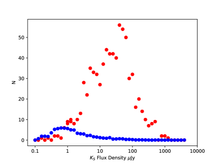
Figure 2: Number of $K_{S}$ sources from Wang et al. [2010] versus $K_{S}$ flux density per logarithmic flux density

bin. Red circles are real identifications. Blue circles are random identifications. The real identifications are plotted as integers. The random identifications have fractional values since the observed values have been scaled down from a much larger area searched as described in the text.

From figure 2 one can see that the plot of the real identifications contains a much larger number of objects than expected number of random sources and the real distribution is shifted to larger flux densities by $\sim 100$ relative to the randoms. Based on figure 2, we set the limiting flux density for IDs in the Wang catalog to $1\mu$Jy, although we will examine the sources with non-IDs based on this limit further using other data. $\sim$95% of the objects in the survey have a identification with a Ks source with a flux density $>1\mu$Jy, near where the random distribution peaks, and thus very few of the IDs can be dominated by a random ID. There are a total of 756 real identifications plotted in figure 2 with $>1\mu$Jy. The sum of the random IDs $>1\mu$Jy, including the statistical error in the mean, is $27\pm 2$ sources or 3.6% of the real sample. Since these should be distributed randomly among the real IDs and non-IDs, one would expect $\sim 1.4$ (5% of 27) of the real IDs with $>1\mu$Jy to be incorrect, random identifications. Furthermore, 95% of the random identifications $<1\mu$Jy must be confused with brighter real IDs.

Given that most of the real IDs are brighter than the typical random source in any error circle, we pick the brighter NIR candidate as the ID in the few cases where more than one object is in the error circle. The Wang catalog becomes incomplete below $1\mu$Jy, so there are more actual weak sources which are confused with a stronger real source inside our search radius. However, only a few of the IDs are mischaracterized by identification found in the Wang catalog. These faint random sources are mostly blended with the real ID, producing small centroid position errors and structure in the NIR images of the real ID. The high identification rate shown in figure 2 compared with the statistical random IDs confirms that the vast majority of the sources in our radio catalog are real.

5.2.2 Nominal non-IDs: further analysis

We then considered the 39/795 radio sources that do not have identifications based on the criteria in the previous section. The properties of these 39 sources are summarized in table 2. Did these objects fail to meet the criteria because there are no associated objects in the NIR surveys or is there some other reason ? In order to study this question we have examined these objects in more detail. All but three have an HST image in at least one band. Eight sources with HST imaging need to be excluded due to various imaging problems documented in table 2. Six are confused by bright sources on the best images, including four with HST images, and could have a faint ID. Two of the objects with HST imaging appear to be blends, based on the size and position angle of the radio source and the location of bright objects in the field. Two are either confused or the correct identification is slightly further from the radio centroid than equation 1 allows.

Taking into account that some of these objects have more than one of the problems listed above, this leaves 30 radio sources with HST imaging (and one without) to be considered. Of these 30, 21 have IDs in at least one of the HST images, closer than criterion given in equation 1, mostly much closer. Estimates were made of expected number of random sources at any detectable brightness using the same technique as for the Wang survey for the four different types of HST images listed in table 2, i.e. using 3^′′ radius circles E, W, N, and S of each source on each type of HST image to estimate the source density of random IDs for each image type. This procedure yielded a total of 0.9 random IDs expected for all 30 error circles combined. This leaves nine radio sources without any ID based on equation 1 and with HST imaging and one without HST imaging, or $\sim 1.3$% of the 787 radio sources without local problems on the images. However, given all the uncertainties discussed and the expectation of one or two random IDs, it seems most likely that less than 2% of individual radio sources do not have an ID at the limit of current optical/NIR data.

Figure 3: The ratio of total flux densities from Morrison et al. [2010] versus those reported in this paper. Only sources with $S/N<20$ in Morrison et al. [2010] are plotted.

5.3 Comparison with The Morrison catalog

Morrison et al. [2010] published a catalog of GOODS-N using images made from data from the old VLA, i.e. before the JVLA upgrades. The spatial resolutions used to analyze the Morrison catalog were similar to the catalog reported in this paper, i.e. $1.7\times 1.6$^′′, 3^′′, and 6^′′ in Morrison. With the best resolution, the rms noise before the primary beam correction was 3.9$\mu$Jy, as compared with 2.2$\mu$Jy for our results with the JVLA. Inside the 9^′ radius circle reported for our new results, there are 484 sources in the Morrison catalog, compared with our 795. In addition, the Morrison data were forced by the parameters of the old VLA correlator to use a much narrower total bandwidth, channel widths of 3.125 MHz and an averaging time of 3 seconds. The individual channels also were almost the same width but not exactly the same shape. These parameters created smearing of the image which increases as one goes away from the pointing/phase center. These effects were approximately taken into account in the Gaussian fitting process but made measurement of the sizes of the sources and thus the total flux densities more difficult. Furthermore, the total bandwidth used in the imaging was only 44 MHz. Besides reducing the sensitivity, the narrow bandwidth produces poorer uv-coverage and thus higher sidelobes for the dirty beam than the new JVLA data.

The Morrison survey did include A, B, C, and D configuration data. However, no very large sources were found. The VLA A-configuration has uv-coverage adequate for minor axis scales up to 36^′′ , so based on the sources found in the Morrison survey, the B, C, and D configurations were not included in this survey.

The median position difference in the sense JVLA-Morrison is about 0.2^′′ in RA and 0.0^′′ in Declination. Since the Wang K-band survey was referenced to the Morrison frame of reference, we have corrected the ID position delta for this difference. It is not clear where the RA difference arises.

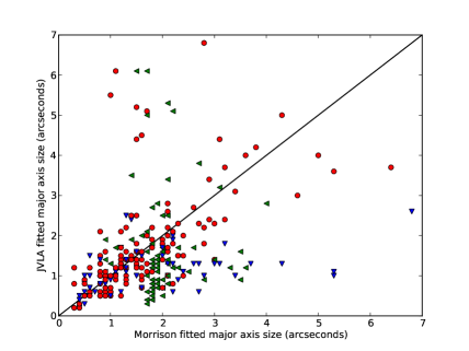
Figure 4: Gaussian major axis sizes from Morrison et al. [2010] versus those reported in this paper. Only sources with both major axis sizes $<7.0$^′′ and a non-upper limit size in one of the two catalogs are plotted. Sources for which both catalogs find the source is resolved are plotted as red dots. Those sources with upper limits in one catalog are plotted as a blue (Morrison catalog) or green triangles (new VLA catalog) with one point of the triangle in the direction of the limit.

In figure 3, we show the ratio of the Morrison et al. [2010] total flux densities to the total flux densities for each source in common between the two surveys with Morrison $S/N<20$. The scatter in the ratio clearly increases at low Morrison S/N. However the median ratio between the two catalogs is 1.06, which is very consistent with the slight difference in the effective frequency of the observations (1400 MHz for Morrison et al. [2010] and 1525 MHz for this survey reported here), given the internal errors, the counting statistics and a mean spectral index in the expected range of $-0.7$ to $-0.8$. Assuming the higher S/N data reported here are correct, it appears that in some cases at low S/N Morrison et al. [2010] finds sources that are spuriously resolved and in other cases misses extended structure. This is just what one might expect at the faint end or “bottom” of a catalog, i.e. near the $5\sigma$ limit and is consistent with the simulations described earlier.

In figure 4 the fitted major axis sizes for sources in both the catalogs are plotted. Only sources found to be resolved in one of the two catalogs are plotted. The plot shows a good underlying correlation between the sizes found, especially if one focuses on the points with measured values in both catalogs, i.e. the red points. As expected the new results find a few sources in the upper left of the plot which are much larger in the new catalog, presumably due to the lower noise and the more extensive search done for resolved sources, i.e. using six resolutions as described in sec. 5.1.1). However, there also is a much larger set of sources significantly below the equal size line. Some of these are upper limits in the Morrison catalog but a significant population is present for which Morrison et al. [2010] found a larger size. A lot of these differences are likely due to the tuning of EFACTOR as discussed above, which was not done for the Morrison et al. [2010] results. The other imaging artifacts, due to the old VLA correlator and the longer averaging times required for the earlier epoch data, must contribute to the differences.

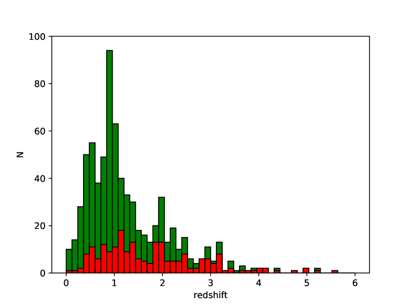
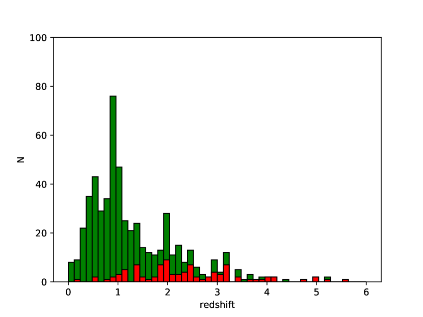
Figure 5: Redshift histograms for full radio survey (left plot) and radio survey with z-band HST imaging (right plot). Green indicates spectroscopic and red indicates photometric redshifts.

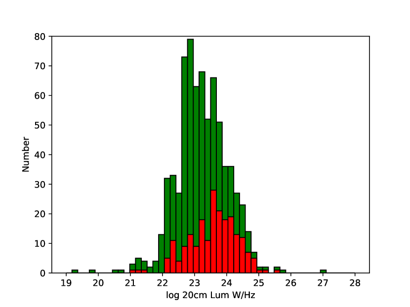
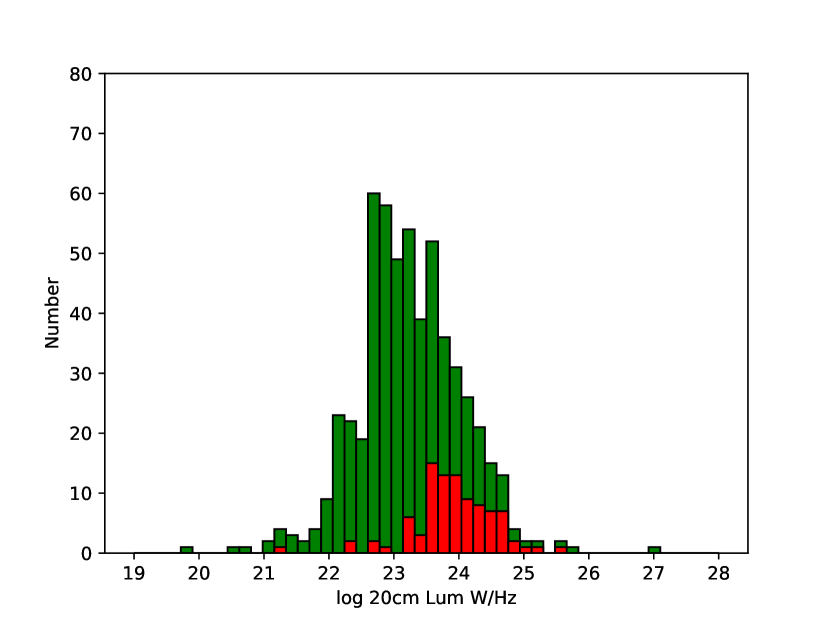
Figure 6: Radio luminosity histograms for full radio survey (left plot) and radio survey with z-band HST imaging (right plot). Green indicates spectroscopic and red indicates photometric redshifts.

At the “bottom” of a catalog, i.e. as one approaches $5\sigma$ detection limit, the ability to measure any information in a given image beyond the peak becomes limited. Unlike Morrison et al. [2010] in the new catalog reported here very few sources have size estimates near this limit as a result of our tuning of the fitting parameters (see fig 7 and section 5.5 below).

5.4 Redshifts, Luminosities

One of the principle reasons to study GOODS-N is the large number of redshifts available for this field. Especially in region of the original GOODS-N HST survey, the number of spectroscopic redshifts is very large. In table 1 the redshifts used and their origin are listed. In figure 5, we plot the histogram of measured redshifts for the full survey and for the subset with z-band HST imaging. The vast majority have spectroscopic redshifts, especially the HST z-band subset. Both redshift distributions peak at $z\sim 1$ with a long tail to higher redshifts.

The completeness level for spectroscopic redshifts, especially for the sample with HST z-band imaging, is very good. In the full survey, there are 520 sources with spectroscopic redshifts, 210 with photometric redshifts and 65 either without redshifts or with no ID. Of those sources with HSTz images, there are 465 with spectroscopic redshifts, 92 with photometric z’s and 26 with no redshifts including those with no ID. In both samples, a large fraction of the $z>2$ redshifts are still based on photometric redshifts.

The corresponding 20cm radio luminosities are plotted in figure 6, assuming $H_{0}=69.6$ $\Omega_{M}=0.286$, $\Omega_{vac}=0.714$. The photometric redshifts contribute a significant fraction of the HST sample at $z\>\hbox{\lower 2.5pt\hbox{$\buildrel>\over{\sim}$}}\>10^{24}$ W Hz^-1. Generally, comparison of the redshifts for radio sources with both photometric and spectroscopic redshifts show that the two estimates agree very well. Also see Yang et al. [2014] from which almost all of the photometric redshifts where taken for a general comparison. However, for the $z>2$ objects, we still have few spectroscopic results. This limits our ability to use spectral lines to help us distinguish between AGN and star-formation as the origin of the radio emission and makes us more dependent on the photometric results for z. The corresponding radio luminosities at which we start to rely on photometric redshifts are also where we might expect a large AGN contribution or perhaps evolution-driven large star-formation rates. So for the higher redshift part of the sample, interpretation becomes harder. For local galaxies, say $z<0.2$, 20cm radio emission is dominated by star-formation for $L_{20}\>\hbox{\lower 2.5pt\hbox{$\buildrel<\over{\sim}$}}\>10^{23}$ W Hz^-1 and by AGN for higher radio luminosities [Condon, Cotton & Broderick, 2002]. For star-formation $10^{23}$ W Hz^-1 corresponds roughly to a star-formation rate of 60 M$\odot$/yr [Yun, Reddy & Condon, 2001, Murphy et al., 2011], slightly below lower limit for ULIRGs ( $L_{FIR}=10^{12}L_{\odot}\sim 100$ M$\odot$/yr; $log(L_{20})\sim 23.25$). A local peak in the histograms shown in figure 6 can be seen, corresponding to $L_{20}\>\hbox{\lower 2.5pt\hbox{$\buildrel<\over{\sim}$}}\>10^{23}$ W Hz^-1 and star-formation rates mostly between 3 and 20 M$\odot$/yr, as is found for low redshift galaxies. Based on this calibration, the majority of the objects in figure 6 must correspond to AGN, or LIRGs ($\sim 10-100$ M$\odot$/yr) and ULIRGs with SFR$\gg 20$ M$\odot$/yr.

5.5 Radio Sizes

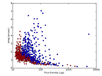
Figure 7: Radio Major Axis Size (bmaj) versus Radio Total Flux Density. Red downward arrows are sources with major axis upper limits. Blue circles are sources with significant measured major axis sizes.

In table 3 we give the list of the deconvolved, fitted Gaussian sizes for each source. In figure 7 we show a plot of these sizes versus total flux density. 346/795 sources, almost half of the total, are found to be resolved. 274 of these have deconvolved resolved sizes with major axes $>1$^′′ and 72 have resolved major axes $\leq 1$^′′. 174 have either upper limits $\leq 1$^′′ (72) or measured resolved sizes, not upper limits, $<1$^′′(102). Since only a minority of the sample have high enough S/N to produce a resolved fit $<1$^′′, we do not try to study these small sources in statistical detail. The remaining 347 sources have upper limits $>1$^′′, we also cannot study the sizes in detail at least at the 1^′′-level. Thus in the rest of this paper we focus mostly on the resolved sources with major axes $>1$^′′ .

The survey is also necessarily incomplete in total flux density due to the small size of the $1.6$^′′ clean beam most often used to set the size limits for weak source, especially at the bottom of the catalog where the S/N is low. Almost all the sources with total flux densities $<20\mu$Jy are not formally resolved (see figure 7), suggesting that some resolved sources in this lower flux density range could be missing and some of the listed sources likely have larger structure. The images were searched for sources at lower resolution but the convolved images have higher noise levels than the 1.6^′′ image. At higher flux densities, the plot shows sources with extended sizes up to $\sim 7$^′′, although the median size below $100\mu$Jy is $<1.5$^′′. The median source size for total flux densities between 10 and 40$\mu$Jy is an upper limit, $<1.7$^′′ . In the 40 to 160 $\mu$Jy range, the median size is 1.3^′′ .

5.6 Comparison of Radio and HST Sizes and Orientations

5.6.1 Radio versus HST Sizes

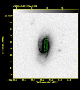
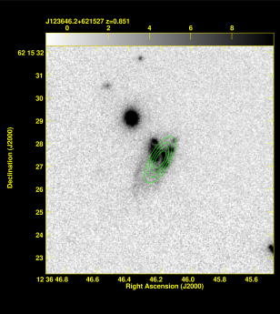
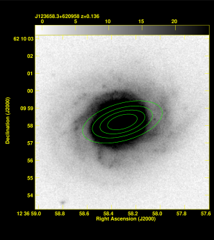
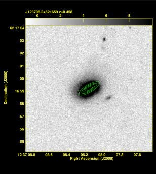
Figure 8: HSTz images with radio models overlaid from table 1 for Individual Galaxies identifications. Fractional contours of $(0.2,0.4,0.6,0.8)\times$ the model peak are plotted.

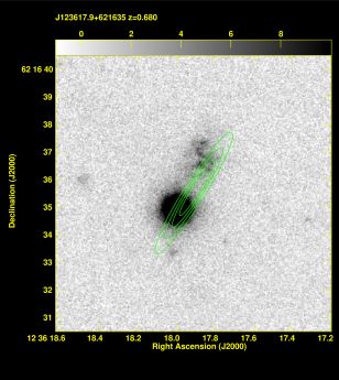
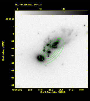
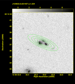
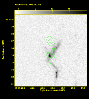
Figure 9: HSTz images with radio models overlayed as contours for Binary or Multiple Galaxy identifications (ID “B” in table 3). Fractional contours of $(0.2,0.4,0.6,0.8)\times$ the model peak are plotted.

For the resolved radio sources it is important to compare their properties with the HST optical imaging [Giavalisco et al., 2004, Koekemoer et al., 2011]. In figures 8 and 9, we display examples of the fitted radio models from table 1 overlaid on the HSTz images. The models, of course, have errors and are an approximation to the true structure so are not expected the line up perfectly. However, one can see the similarity to the optical structure.

For the binary systems, the sizes tend to be small, supposedly because the larger binaries would likely be measured as two separate identifications. For the multiple systems the measured size is the distance between the centers of the outer components of the system. The models are an approximation to the actual, often much more complicated brightness distribution. In figure 9, J123633.0+621437 is an example of a fit that suggests the brightness distribution extends beyond the three galaxies. On the other hand, the model for J123650.4+622035 is centered near the galaxy near the field center but is not aligned with that galaxy. Instead the alignment fits with the PA of more southern components of the multiple system. We have interpreted the extended source as due to the multiple system with some unknown more complex structure, instead of being an extended misaligned source associated with a single galaxy.

For sources with HSTz data sizes $>1$^′′ (169 sources), we have measured the largest isophotal size of the galaxy and multiple/binary galaxy IDs on the HSTz images, i.e. the isophote at which the galaxy brightness blends into the noise. This “lowest” isophote was used for consistency and because the lowest isophote gives the largest lever arm for measuring the orientation of the galaxy. In practice the vast majority of the galaxies had very similar position angles for the inner and outer structure.

In table 3 we list the measured radio and HSTz optical sizes and position angles for the 169 radio sources with deconvolved major axis sizes $>1$^′′. In figure 10 we plot the radio versus optical sizes for those 169 sources. In most cases the individual optical galaxies measured this way are larger than the radio sources by about $1.5\times$ in the median. For multiple/binary optical systems are slightly smaller than the radio major axes, $\sim 0.8\times$ in the median. Note that we are measuring very different quantities for the size, so we should not expect perfect agreement. The radio Gaussian size is a proxy for the 2nd moment. The optical isophotal size is a function of redshift due to the cosmological $(1+z)^{4}$ isophotal dimming and the redshifting of the z-band below the 4000Å break for $z\>\hbox{\lower 2.5pt\hbox{$\buildrel>\over{\sim}$}}\>1$. Most of the galaxies appear to be disks but not all, so the significance of the size measured from outer isophote will be different for the early-type systems.

Table 3: Radio and HSTz optical position angles for sources with radio major axes $>1$^′′

^a Name ID R PA Err Res O PA R Si O Si (1) (2) (3) (4) (5) (6) (7) (8) J123541.4+621217 G 133 16 1.6 125 3.2 4.2 J123546.7+621048 G 78 25 1.6 98 1.6 2.4 J123553.1+621073 G 146 15 1.6 6 1.4 2.1 J123553.1+620954 B 161 41 1.6 24 1.4 3.4 J123554.0+621043 G 150 17 1.6 146 1.1 6.2 J123558.1+621355 G 110 31 6.0 119 6.1 4.5 J123559.7+621549 G 44 8 1.6 39 1.6 6.6 J123600.4+621053 G 25 39 1.6 51 2.5 0.8 J123601.1+621058 G 13 15 1.6 172 1.9 3.0 J123605.4+621031 G 39 11 1.6 30 2.7 2.4

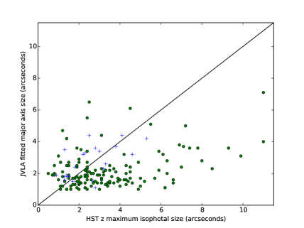
Figure 10: VLA deconvolved Gaussian major axis (FWHM) versus maximum isophotal HST z-band major axis for radio sources with sizes $>1\hbox{${}^{\prime\prime}$}$ identified with individual galaxies (green circles) and binary systems (blue pluses).

A small number of galaxies have smaller optical sizes than the radio sources. About two thirds of these have $z>1$ and are small, $<1.5$^′′, perhaps due to the redshift dependent effects discussed above. At $z>1$ the radio luminosities are also larger, $>10^{23}$ W Hz^-1, thus some may be AGN. One in particular, J123644.4+621133, is $43$^′′ in radio size and is clearly an FRI.

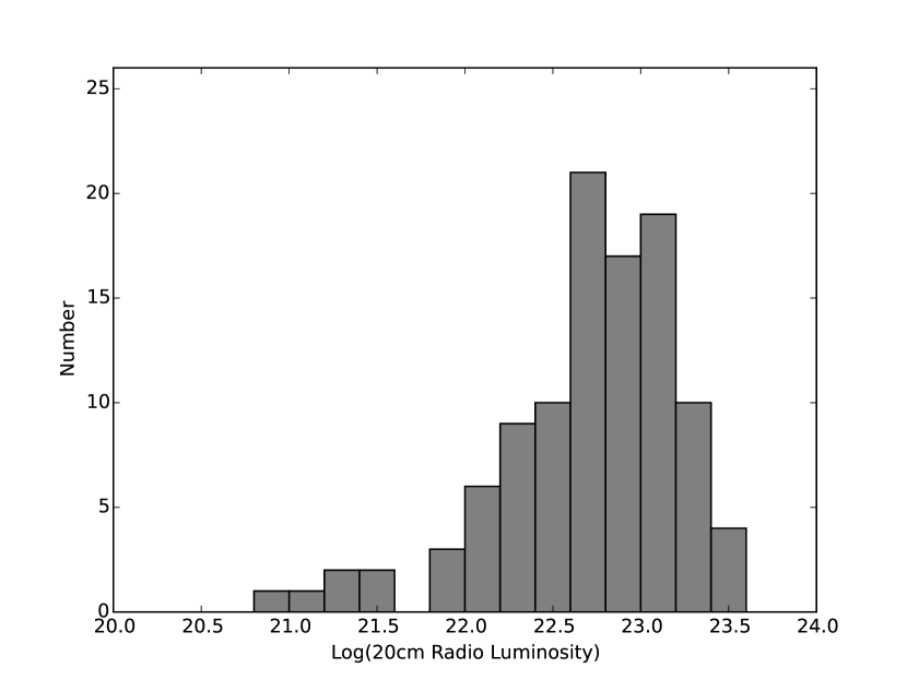
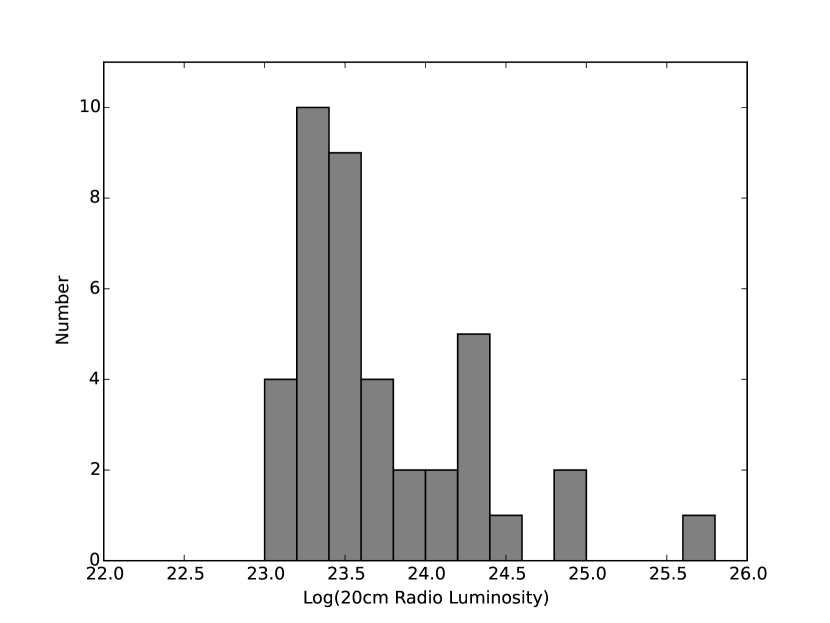
Figure 11: Radio Luminosities for sources with HST z imaging and radio sizes $>1\hbox{${}^{\prime\prime}$}$: left) $z<1$ (left plot), $z>1$ (right plot). Note the split between the two samples very near $L_{20}=10^{23}$ W Hz^-1. Locally $10^{23}$ W Hz^-1 is the dividing point between dominance by star-forming galaxies and dominance by AGN.

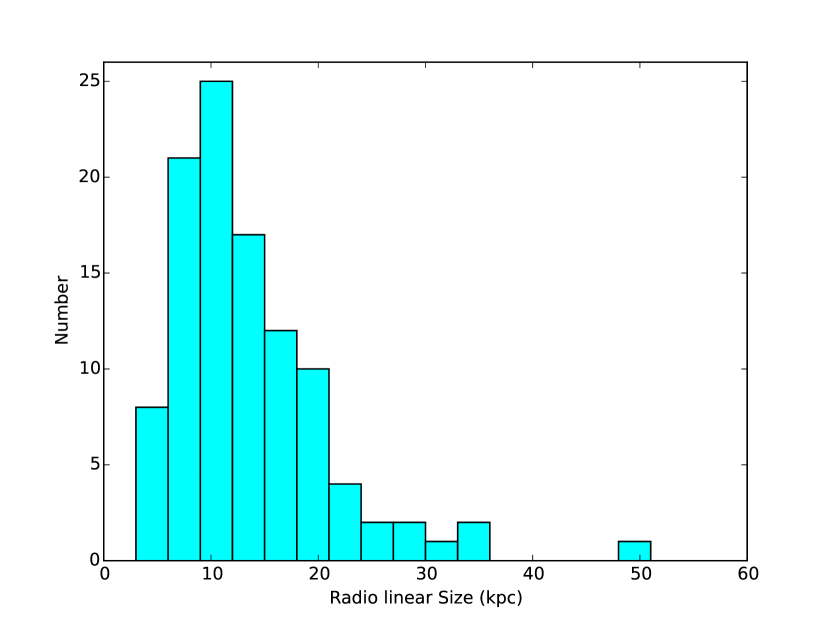
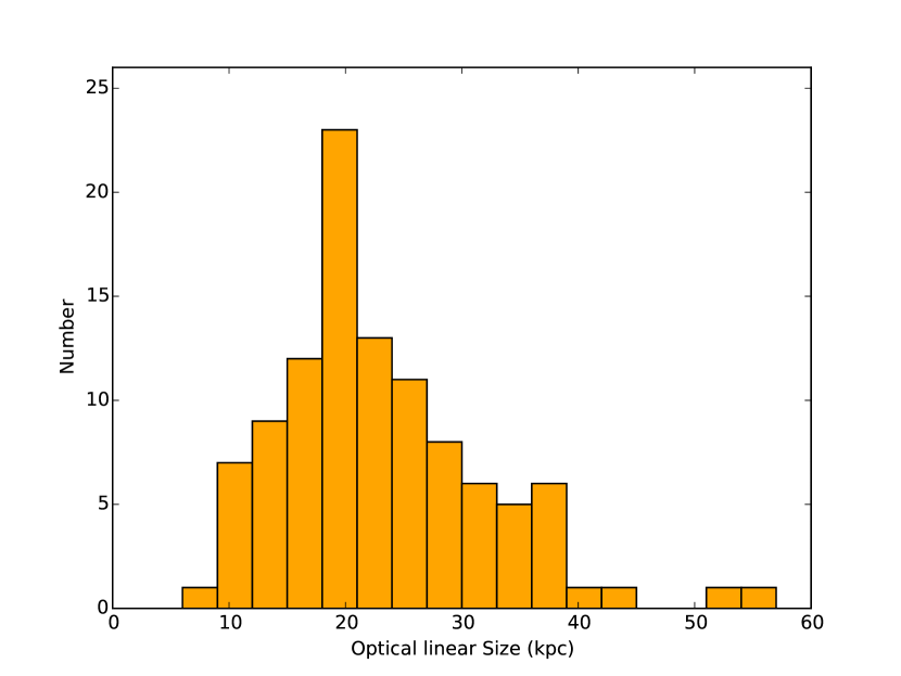
Figure 12: Radio Galaxies with HST z imaging, sizes $>1\hbox{${}^{\prime\prime}$}$ and $z<1$: radio Gaussian major axes (left plot), optical isophotal major axes (right plot). The optical sizes show that these galaxies are much larger than local ULIRGs, suggesting that that the radio size selection picks out such monolithic systems. The radio sources, while larger than the nuclear region, are systematically smaller than the optical isophotal size, showing they are contained inside their associated galaxies.

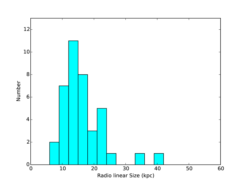
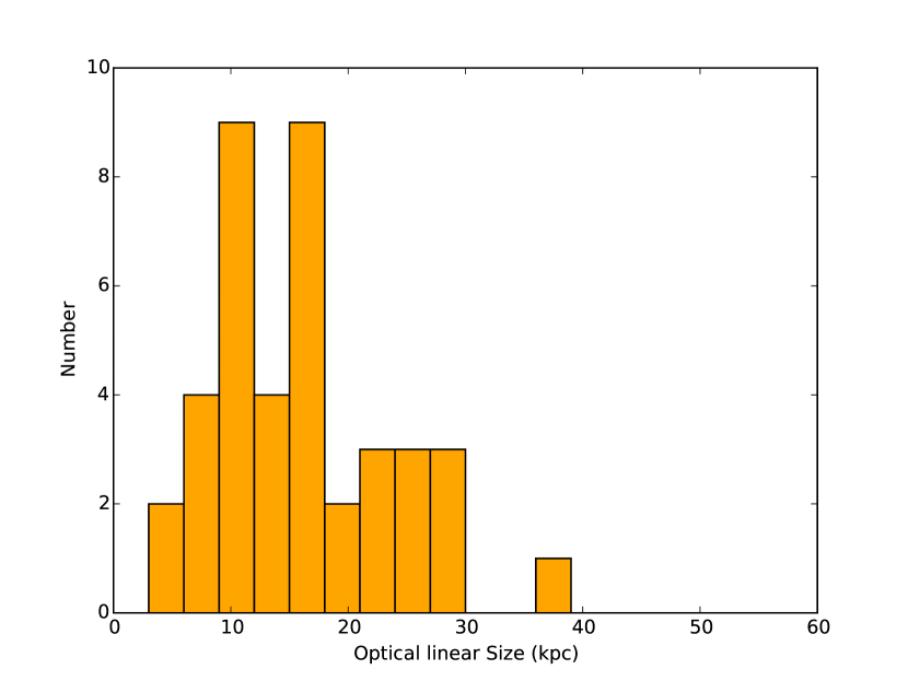
Figure 13: Radio Galaxies with HST z imaging, sizes $>1\hbox{${}^{\prime\prime}$}$ and $z>1$: radio Gaussian major axes (left plot) and optical isophotal major axes (right plot). For $z>1$ unlike $z<1$, the radio and optical sizes are similar, perhaps due to the cosmological effects on the optical isophotes.

In figure 11 histograms of the radio luminosity are plotted for galaxies with sizes $>1$^′′ splitting the population into $z<1$ and $z>1$. This divides the sample by luminosity very close to $log(L_{20})=23$, which locally is the dividing line between the vast majority of the radio sources being star-forming for lower luminosities and being AGN for higher luminosities [e.g. Condon, Cotton & Broderick, 2002].

For sources identified with individual galaxies with sizes $>1$^′′, 107/147 have $z<1$, where $z=1.01$ is the median redshift for the radio sources so far measured (the vast majority). Thus these resolved individual galaxies tend to be at the lower redshifts, corresponding to lower radio luminosities. The median redshift for the $z<1$ sample is 0.56 and the median $log(L_{20})=22.77$. Assuming star-formation is the origin of the radio emission, most of the objects are in the LIRG class and about 10% extend into the ULIRG class. Forty individual galaxies are found with $>1$^′′ and $z>1$. The redshifts are mostly $<1.5$ with a tail extending up to almost $z=4$. Assuming the local star-formation relation, radio luminosities are all in the ULIRG class.

In figure 12 we show histograms of the radio and optical sizes from table 4. For $z<1$ the radio sizes have a median of 11.6 kpc, while the median optical size is 21.5 kpc. Thus the radio emitting region extends well outside the galaxy nucleus but is typically less than than half our measured optical isophotal size. These galaxies, selected by picking radio sources $>1$^′′ , are large, grand-design spirals or disk galaxies with isophotal diameters up to 60kpc. They are unlike the local population of ULIRGs, which are much smaller, disturbed systems dominated by nuclear starbursts and the associated compact radio emission [e.g. Condon et al., 1991, Rujopakarn et al., 2011, Barcos-Muñoz et al., 2015]. While this is a subset of the $\sim 400$ sources with $z<1$, it is a large subset and shows that a significant fraction of sources have extended emitting regions outside the nucleus. Furthermore, typically the unresolved sources have upper limits to the radio size, $\sim 10$ kpc. Thus it is likely that more of the galaxies have extended emitting regions outside the nucleus than the subset we have identified. The vast majority of the identifications appear to be disk galaxies, thus it appears that many of the disks are emitting and that the star-formation is not limited to a nuclear star-burst for a significant fraction of the $z<1$ galaxies in the sample.

For 39 radio galaxies with $>1$^′′ and $z>1$, we display their radio and optical size in figure 13. One object, J123644.4+621133, is not plotted since it is too big to fit on the radio size plot and is clearly an AGN based on its radio morphology. The radio and optical sizes are similar with a median near 15 kpc. Of course, the optical sizes are affected by the isophotal dimming due to both cosmological effects and the redshifting of the z filter response. In the HSTz images for $z<1.2$ many of the IDs are clearly spiral or disk galaxies. This result is consistent with most of the galaxies in the sub-sample being due to star-formation. Beyond $z\sim 1.2$, as the z filter is redshifted further to the blue and beyond the 4000Å break , the galaxy morphologies become less clear. Mostly the objects appear to be an extension of the upper end of the $z<1$ sample up to $z\sim 1.2$ but the nature of the $z>1.2$ objects becomes less clear based on this analysis. However, Barger et al. [2015] shows that for this same, full sample, except for the the most luminous X-ray sources ($L_{X}>5\times 10^{43}$ ergs s^-1), the radio sources fit the radio-FIR relation. This result suggests that the typical radio source in our full radio sample, out to $z\sim 4$, is due to star-formation.

Twenty-two radio sources with sizes $>1$^′′ are classified as binaries (or multiple systems). These systems have similar radio and optical sizes with medians $\sim 20$kpc. Of course their definition is largely dependent on the survey resolution, since much smaller objects would be unresolved and much larger objects would be cataloged as individual galaxies. Their median redshift is near $z=1$ and their median $log(L_{20})=23.26$. Thus they appear unremarkable except that they contribute about 10% to the resolved radio source sample.

5.6.2 Radio versus HST Orientations

It is also important to compare the orientations of the radio emission and optical isophotes. For sources sizes $>1$^′′, we remeasured the position angle of the radio emission using JMFIT in order to obtain the best estimate of the position angle. Sometimes the smallest position angle error was obtained using an image with a slightly different resolution than was used in the main catalog. We also measured the optical position angles for the corresponding optical identifications for the outer visible isophotes on HST images. For the HST images, we used the z-band. The position angles and sizes were measured down to the faintest isophote easily visible above the noise. This scale tends to be larger than what one often picks as the extent of the disk but is well defined on the images and mostly aligns with any smaller scale disk. Typically we estimate that we measured the optical position angle to within 10 degrees. These results are summarized in table 3. For sources with JMFIT errors $<20$ degrees, we plot in figure 14 the position angle differences. 74% of the resulting sample are aligned within 30 degrees. In the majority these cases, the identification is clearly a disk galaxy. Thus these extended systems appear to have emission aligned with the disk, likely from star-formation along the disk.

The remaining 24%, apparently misaligned sources, show no outstanding common property and are likely due to a combination of effects. Three are very low S/N, $\leq 5.3$, and based on the simulations could be spurious resolved sources. Three more have S/N between 6.2 and 6.7. The median S/N is 9.1, with one as high as 75. Two appear to be associated with E-galaxies and thus are AGN candidates. One is aligned with an inner structure but not with outer spiral arms. Most appear to be disk galaxies, without obvious alignment with any features in the image.

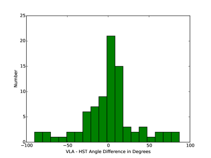
Figure 14: Difference in orientation angles for VLA radio sources with deconvolved sizes $>1\hbox{${}^{\prime\prime}$}$ identified with individual galaxies versus orientation of the identifications from HSTz images. Only radio sources with orientation errors less than 20 degrees are included.

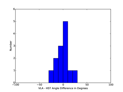
Figure 15: Difference in orientation angles for individual VLA sources identified with multiple galaxies (mostly binaries) and with radio sizes $>1\hbox{${}^{\prime\prime}$}$ in fitted size versus orientation of the identifications from HSTz images. Only radio sources with orientation errors less than 20 degrees are included.

In figure 15, we show a similar plot for radio sources identified with binary galaxies (or multiple systems, mostly binaries). Here the alignment is even better. In addition to these close binaries, there is a small sample of larger-scale blends discussed in the previous section. For other sources $>1$^′′, there is some reason which prevents us from making a radio-optical comparison. Either the optical identification is too small or the radio or optical object is too round to measure an orientation accurately. There is a tendency for the galaxies imaged with HST z-band in these multiple systems to be smaller than the IDs with single galaxies. The median isophotal size for the larger of the two optical galaxies in binaries is only $\sim 10$kpc. These smaller galaxies in binaries also appear usually to have dust obscuration in the nuclear region. 7/8 of the systems with its larger galaxy $>15$ kpc have $z<1$ and 6/8 have $\log(L_{20})<23$. For the 14 smaller systems 13/14 have $z>1$ and $\log(L_{20})>23$.

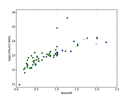
Figure 16: Luminosity versus redshift for VLA sources $>1\hbox{${}^{\prime\prime}$}$ identified with individual galaxies (green circles) and binary systems (blue circles). Filled circles have spectroscopic redshifts, open circles have photometric redshift. Only radio sources with orientation errors less than 20 degrees and absolute Radio-HST position angle difference less than 30 degrees are plotted. The LIRG/ULIRG boundary is $log(L_{20})\sim 23.25$.

In figure 16, the radio luminosity versus redshift is plotted for galaxies and binaries with which have radio position angle errors from AIPS JMFIT $<20$° and which are aligned to within better than 30°. As can be seen in the plot the aligned sample extends well beyond the LIRG luminosity cutoff into the ULIRG class and generally has typical luminosities near the LIRG/ULIRG luminosity boundary.

The conclusion is that, at least for $z\>\hbox{\lower 2.5pt\hbox{$\buildrel<\over{\sim}$}}\>1$, the radio sources in the survey with structure $>1$^′′ tend to be either large galaxies in the LIRG/ULIRG class with disk emission on scales outside their nuclear regions likely driven by star-formation, or multiple galaxy systems.

6 Discussion

The median redshift for sources with measured redshifts for the survey ($z=1.01$) marks a useful dividing point for understanding the properties of the sources. For $z<1$, 68% of the sources have $\log(L_{20})$ between 22 and 23. 8% have radio luminosities below this range and 24% above. For star-forming galaxies this range corresponds roughly to LIRGs. As discussed earlier, locally it is well known that at $\log(L_{20})<23$, the radio luminosity from galaxies is dominated by star-formation [e.g. Condon, Cotton & Broderick, 2002]. Thus 76% of the lower redshift half of the survey have luminosities in the range locally dominated by star-formation and most of those are in the range occupied by strongly star-forming galaxies but not objects in the ULIRG class. Examination of the HST images reveals many, perhaps most, of these objects appear to be dusty disk galaxies, very consistent with strong star formation. For those that have high enough S/N so that a size and position angle can be measured, the radio emission is statistically aligned with the optical major axis (figure 14). Figure 7 suggests that at the bottom of the catalog, we are likely underestimating the flux densities of such galaxies and missing a significant number of them since we are resolving them and cannot measure a statistically significant size. However, the ones we can analyze suggest that much of the disk is emitting star-formation-driven radio emission. Figure 16 shows that most of the radio-optical aligned galaxies we have found have $z\>\hbox{\lower 2.5pt\hbox{$\buildrel<\over{\sim}$}}\>1$.

Above $z=1$, only about 6% of the sources have $\log(L_{20})<23$. The median redshift is 1.7. The median $\log(L_{20})$ is 23.72, corresponding to $\sim 300$ M$\odot$/yr. 32% have $\log(L_{20})>24$ suggesting either SFR $>500$ M$\odot$/yr, AGN-related emission, a combination of AGN/star-formation or perhaps some other physics is involved. A few very large, luminous sources are clearly AGN, based on their radio structure, but the rest need other information to understand them, e.g. Barger et al. [2015]. Furthermore Barger et al. [2017] find that for $z>0.8$, $\sim 40$% of the radio sources in our GOODS-N sample with $\log(L_{20})>24$ are consistent with star-formation, based on comparison of the radio and submillimeter flux densities. The rest show some evidence of an AGN contribution. Especially for $\log(L_{20})>24.5$, all the sources appear to be AGN suggesting a cutoff in the maximum SFR at $\sim 500$ M$\odot$/yr.

Besides the “standard” radio population there clearly are some other origins of sources in the table. Small subsets are either binary galaxies with both members emitting or blends of emission from two or more apparently unrelated galaxies. There also is a small population of sources without identifications. Objects so faint seem likely to be very high z and/or very dusty galaxies. If AGN-driven bubble sources or star-forming radio galaxies dominated by wind-related emission were important, we would have expected a significant number of diffuse sources not aligned with the optical galaxy axis and often larger than the optical galaxy image. We do not find such populations. It remains possible that they remain hidden due to the star-formation-driven or AGN-driven emission dominating the regions imaged. At the sensitivity level of this survey, star-formation and some AGN activity, especially at higher redshifts, seem to dominate the observed radio emission.

The most surprising result is the statistical alignment of the sources $>1$^′′ in size with the extended optical disks, especially with $z<1$. This implies that there is a significant population of galaxies in the LIRG/ULIRG class which are not dominated by nuclear star-formation but have most of their star-forming radio emission extended along the galaxy disk, typically $\sim 10$kpc. What fraction of all the radio galaxies in the survey have this extended star-forming emission is hard to pin down because for the weaker cataloged sources the S/N, even given the convolved searches, would not be adequate to measure the extensions at significant levels. Deeper surveys are needed to study this problem.

This division into two redshift ranges does not suggest necessarily that there is a fundamental change in the radio source populations at $z=1$, only that the survey selection effects produce such a division. This survey is not deep enough to study the LIRG population much beyond $z=1$. The resolution and surface brightness sensitivity is just high enough to to resolve a significant fraction of the sources. Since locally such sources show extended winds which emit in the radio with steep radio spectral indices, higher rest-frame frequencies may miss that part of the story, especially for higher redshifts. Combined with the limited surface brightness sensitivity even at 1.5GHz we may be missing a lot at the higher rest frequencies especially for $z>1$. Deep surveys at lower frequencies would be a useful check.

7 Conclusions

A new radio catalog based on a deep, 1525 MHz VLA radio image ($2.2\mu$Jy rms near the field center of the 1.6^′′ image) is reported, along with its properties, including optical/NIR identifications. 795 sources were detected within 9^′ of the nominal GOODS-N center position. With modern ground-based NIR imaging depths and with HST optical imaging, the vast majority of radio sources with at our radio limits have been identified reliably with $<2$% of the sources remaining unidentified or misidentified. Especially for $z<1$, a large subset of the survey has radio sizes $>1$^′′ . The size and alignment of the radio emission for those sources with the HST images of disk galaxies suggests that there is a large population of LIRG/ULIRGs, with most of their star-formation not isolated in the galaxy nucleus, but with strong star-formation extending along the 10kpc-scale disk. This survey naturally divides at the median redshift near $z=1$, into 1) a $z<1$ population mostly very consistent with strongly star-forming disk galaxies and many with resolved star-forming regions and 2) a $z>1$ sample typically with much higher SFRs and/or AGN emission.

8 Acknowledgments

This research has made use of the VizieR catalogue access tool, CDS, Strasbourg, France. The original description of the VizieR service was published in A&AS 143, 23.

The HST GOODS-N cutout images presented in this paper were obtained from the Mikulski Archive for Space Telescopes (MAST). STScI is operated by the Association of Universities for Research in Astronomy, Inc., under NASA contract NAS5-26555. Support for MAST for non-HST data is provided by the NASA Office of Space Science via grant NNX09AF08G and by other grants and contracts.

The author thanks Bill Cotton, Emanuele Daddi, Jean Eilek and Ken Kellermann for comments on the text.

References

- Adebhar et al. [2013] Adebahr, B., Krause, M., Klein, U. et al. 2013, A&A, 555, a23.
- Barcos-Muñoz et al. [2015] Barcos-Muñoz, L., Leroy, A. K., Evans, A. S. et al. 2015,ApJ, 799, 10.
- Barger et al. [2003] Barger, A.J., Cowie, L. L., Capak, P. et al 2003, AJ, 126, 632.
- Barger, Cowie & Wang [2008] Barger, A. J., Cowie, L. L. & Wang, W.-H. 2008, ApJ, 689, 687.
- Barger et al. [2012] Barger, A. J., Wang, W-H., Cowie, L. L., et al 2012, ApJ, 761, 89.
- Barger et al. [2014] Barger, A. J., Cowie, L.L., Chen, C. C. et al. 2014, ApJ, 784, 9.
- Barger et al. [2015] Barger, A. J., Cowie, L. L., Owen, F. N. et al 2015, ApJ, 801, 87.
- Barger et al. [2017] Barger, A.J., Cowie, L. L., Owen, F. N. et al. 2017, 835, 95.
- Chyzy & Beck [2004] Chyzy, K. T. & Beck, R. 2004, A&A, 417, 541.
- Chapman et al. [2005] Chapman, S. C., Blain, A. W., Smail, I. & Ivison, R. J. 2005, ApJ, 622, 772.
- Condon [1992] Condon, J. J. 1992, ARA&A, 30, 575.
- Condon et al. [1991] Condon, J. J., Huang, Z.-P., Yin, Q. F., & Thuan, T. X. 1991, ApJ, 378, 65.
- Condon, Cotton & Broderick [2002] Condon, J. J., Cotton, W. D. & Broderick, J. J. 2002, AJ, 124, 675.
- Condon, Helou, & Jarrett [2002] Condon, J.J., Helou, G. & Jarrett, T.H. 2002,AJ, 123, 1881.
- Cowie et al. [2004] Cowie, L. L., Barger, A. J., Hu, E. M., Capak, P. & Songaila, A. 2004, AJ, 3137.
- Cowie et al. [2017] Cowie, L. L., Barger, A. J., Hsu, L.-Y. et al. 2017, ApJ, 837, 139.
- Dickinson et al. [2003] Dickinson, M., Papovich, C., Ferguson, H. C. & Budavári, T. 2003, ApJ, 587, 25.
- Giavalisco et al. [2004] Giavalisco, M., Ferguson, H. C., Koekemoer, A. M. et al. 2004, ApJ, 600, L93.
- Lui et al. [2017] Lui, D., Daddi, E., Dickinson, M. et al. 2017, arXiv170305281L
- Koekemoer et al. [2011] Koekemoer, A. M., Faber, S. M., Ferguson, H. C. et al. 2011 ApJS, 197, 36.
- Martin et al. [2012] Martin, C. L., Shapley, A. E., Coil, A. L., et al. 2012, ApJ, 760, 127.
- Momcheva et al. [2016] Momcheva, I. G, Brammer, G. B., van Dokkum, P. G. et al. 2016 ApJS, 225, 27.
- Morrison et al. [2010] Morrison, G. E., Owen, F. N., Dickinson, M., Ivison, R. J. & Ibar, E. 2010, ApJS, 188, 187.
- Murphy et al. [2011] Murphy, E. J., Condon, J. J., Schinnerer, E. et al. 2011, ApJ, 737, 67.
- Muxlow et al. [2005] Muxlow, T. W. B., Richards, A. M. S., Garrington, S. T. et al. 2005, MNRAS, 358, 1159.
- Owen, Eilek & Kassim [2000] Owen, F. N., Eilek, J. A. & Kassim, N. E. 2000, ApJ, 543, 611.
- Pannella et al. [2015] Pannella, M., Elbaz, D., Daddi, E. et al. 2015, ApJ, 807, 141.
- Pfrommer [2013] Pfrommer, C. 2013, ApJ, 779, 10.
- Rau & Cornwell [2011] Rau, U. & Cornwell, T. J. 2011, A&A, 532, A71.
- Rau, Bhatnagar & Owen [2016] Rau, U., Bhatnagar, S & Owen, F. N. 2016, AJ, 152, 164.
- Reddy et al. [2006] Reddy, N. A., Steodel, C. C., Erb, D. K., Shapley, A. E. & Pettini. M. 2006, ApJ, 653, 1004.
- Richards [2000] Richards, R. E. 2000, ApJ, 533, 611.
- Rujopakarn et al. [2011] Rujopakarn, W., Rieke, G. H., Eisenstein, D. J. & Juneau, S. 2011, ApJ, 726, 93.
- Rudnick & Owen [2014] Rudnick, L. & Owen, F. N. 2014, ApJ, 785, 45.
- Seaquist & Odegard [1991] Seaquist, E. R. & Odegard, N. 1991, ApJ, 369, 320.
- Skelton et al. [2014] Skelton, R. E., Whitaker, K. E., Momcheva, I. G., Brammer, G. B., Dokkum, P. G. et al. 2014, ApJS, 214, 24.
- Strazzullo et al. [2010] Strazzullo, V., Pannella, M., Owen, F. N. et al. 2010, ApJ, 714, 1305.
- Sutherland & Saunders [1992] Sutherland, W. & Saunders, W. 1992, MNRAS, 259,413.
- Tan et al. [2013] Tan, Q., Daddi, E., Sargent M. et al 2013, ApJ, 776, 24.
- Tan et al. [2014] Tan, Q., Daddi, E., Magdis, G. et al 2013, å, 569, 98.
- To, Wang & Owen [2014] To, C-H., Wang, W-H. & Owen, F. N. 2014, ApJ, 792, 139.
- Vernstrom et al. [2016] Vernstrom, T., Scott, D., Wall, J. V. et al. 2016, MNRAS, 462, 2934.
- Walter et al. [2012] Walter, F. DeCarli, R., Carilli, C. et al. 2012, Nature, 486, 233.
- Wang et al. [2010] Wang, W.-H., Cowie, L. L., Barger, A. J., Keenen, R. C., & Ting H.-C. 2010, ApJS, 187, 251.
- Williams et al. [1996] Williams, R. E. et al. 1996, AJ, 112, 1335.
- Wirth et al. [2015] Wirth, G. D., Trump, J. R., Barrow, G. et al. 2015, AJ, 150, 153.
- Yang et al. [2014] Yang, G., Xue, Y. Q., Luo, B. et al. 2014, ApJS, 215, 27.
- Yun, Reddy & Condon [2001] Yun, M. S., Reddy, N. A. & Condon, J. J. 2001, ApJ, 554, 801.