Detection of HOCO⁺ in the protostar IRAS 16293-2422

Abstract

The protonated form of CO₂, HOCO⁺, is assumed to be an indirect tracer of CO₂ in the millimeter/submillimeter regime since CO₂ lacks a permanent dipole moment. Here, we report the detection of two rotational emission lines (4_0,4–3_0,3 and 5_0,5–4_0,4) of HOCO⁺ in IRAS 16293-2422. For our observations, we have used EMIR heterodyne 3 mm receiver of the IRAM 30m telescope. The observed abundance of HOCO⁺ is compared with the simulations using the 3-phase NAUTILUS chemical model. Implications of the measured abundances of HOCO⁺ to study the chemistry of CO₂ ices using JWST-MIRI and NIRSpec are discussed as well.

1 Introduction

Dust grains in the interstellar medium (ISM) are coated mostly with H₂O, CO, CO₂ ices along with other minor ice constituents formed in particular by surface chemistry. In star forming regions, these ices account for up to 60 and 80 percent of the volatile oxygen and carbon budget (Öberg et al., 2011). CO₂ is an important constituent of these ices. CO₂ ice has been observed in dense clouds (Whittet et al. (1998); Bergin et al. (2005); Knez et al. (2005); Whittet et al. (2009); Noble et al. (2013)), protostellar envelopes (Noble et al. (2013); Boogert et al. (2004); Pontoppidan et al. (2008); Shimonishi et al. (2010); Aikawa et al. (2012)) and in comets (Ootsubo et al., 2012), the remnants of the proto-Solar Nebula. Irrespective of the different astrophysical sources, its abundance with respect to H₂O is constant around 20-30%, which is one of the biggest puzzle for the astronomers (see below).

In the literature, many plausible scenarios have been proposed to explain the formation of CO₂ ice in the ISM (Pontoppidan et al., 2008). D’Hendecourt et al. (1985) have suggested that strong UV irradiation is needed to produce the observed CO₂ ice since the reaction CO + O$\rightarrow$CO₂ on the surface has a large activation barrier. Later, D’Hendecourt et al. (1986) confirmed from laboratory experiment that CO₂ is formed from the ice mixtures of H₂O and CO under strong UV photolysis. The detection of CO₂ ice around UV-luminous massive young stars has confirmed this laboratory experiment (Pontoppidan et al. (2008) and reference therein). But the detection of CO₂ ice in dark clouds with similar abundances (Bergin et al. (2005); Knez et al. (2005)) has questioned the UV irradiation route to CO₂ since these sources are far away from any ionizing source. Later, with the help of a laboratory experiment, Roser et al. (2001) claimed that the barrier for the oxygenation of CO is much lower than previously assumed. Theoretical calculations and laboratory experiments are still a very active topic to understand the formation of CO₂ ice in the ISM (Cooke et al., 2016).

Through chemical models, CO₂ is also predicted to be one of the more abundant carbon and oxygen bearing molecules in the gas phase (Herbst & Leung (1989); Millar et al. (1991)). In the solid phase, the observed abundance for CO₂ is of the order of $10^{-5}$ to $10^{-6}$ relative to H₂ (Gerakines et al., 1999), e.g. a factor of 10 to 100 higher than in the gas phase (van Dishoeck et al. (1996); Boonman et al. (2003)). The large amount of CO₂ in the gas phase could be produced by the evaporation or destruction of the icy grain mantles (van Dishoeck et al., 1996). Comparing the observed gas and ice phase CO₂ abundance ratio with those of other species (e.g. H₂O; CO) known to be abundant in icy mantles, will allow us to understand the formation mechanisms of CO₂.

Carbon dioxide cannot be observed in the gas phase through rotational transitions in the far-infrared or submillimeter range due to its lack of permanent dipole moment. It has to be observed through its vibrational transitions at near- and mid-infrared wavelengths. The protonated form of CO₂, HOCO⁺ , is an interesting alternative to track the gas phase CO₂ in the millimeter/submillimeter regime. According to Herbst et al. (1977), the abundance of gas phase CO₂ relative to CO might be constrained by comparing the abundance of HOCO⁺ with that of HCO⁺. HOCO⁺ was first detected in Galactic centre cloud SgrB2 (Thaddeus et al., 1981) and later towards SgrA (Minh et al., 1991). HOCO⁺ was also detected in low-mass Class 0 protostar IRAS 04368+2557 in L1527 (Sakai et al., 2008); in the prototypical protostellar bow shock of L1157-B1 (Podio et al., 2014); recently in L1544 prestellar core (Vastel et al., 2016).

In this paper, we report the first detection of HOCO⁺ in the low mass protostar IRAS 16293-2422 (hereafter IRAS 16293) and discuss its astrochemical implications as an indirect tracer of gas phase CO₂.

2 Observations and data reduction

2.1 Observations

The observations were performed at the IRAM-30m towards the midway point between sources A and B of IRAS 16293 at $\alpha_{2000}=16^{h}32^{m}22.75^{s},\delta_{2000}=-24\degr 28\arcmin 34.2\arcsec$. We preformed our observations during the period of August 18 to August 23, 2015 under average summer conditions (a median value of 4-6 mm water vapour). For our observations, we have used the EMIR heterodyne 3 mm receiver tuned to a frequency of 89.98 GHz in the Lower Inner sideband, connected to the FTS spectrometer in its 195 kHz resolution mode. Our observed spectra was composed of two regions: one from 84.4 GHz to 92.3 GHz and another one from 101.6 GHz to 107.9 GHz.

Figure 1: The red lines show the observed lines attributed to HOCO⁺. The black lines show the distribution of modelled spectra following the posterior distribution of parameters shown in Fig. 2. The thick line denotes the median of the distribution. The dark and light grey regions show the 68% and 95% confidence intervals. The dotted lines are 1$\sigma$, 3$\sigma$ and 5$\sigma$ noise levels. 1$\sigma$ level is 2.7 mK.

2.2 Results

Table 1: Observed lines and spectroscopic parameters^‡ for HOCO⁺

Transitions	Frequency	Aij	Eup	VLSR	FWHM	Integrated flux
	(MHz)	(s-1)	(K)	(km s-1)	(km s-1)	(K km s-1)
40,4–30,3	85531.497	2.36$\times$10-5	10.3	4.06 $\pm$ 0.11	0.69 $\pm$ 0.03	0.015 $\pm$ 0.004
50,5–40,4	106913.545	4.71$\times$10-5	15.4	4.16 $\pm$ 0.09	0.94 $\pm$ 0.04	0.020 $\pm$ 0.004

^‡Spectroscopic data have been taken from Bizzocchi et al. (2017)

2.2.1 HOCO⁺ line properties

We have used the CLASS software from the GILDAS package for our data reduction and analysis. We did Gaussian fits to the detected lines after subtracting a local low (0 or 1) order polynomial baseline subtraction. In Table 1, we have shown the result of these fits for the two detected lines of HOCO⁺. Both these detected lines are single-component features with mean LSR velocity of $\sim$ 4.1 km/s and a mean FWHM of $\sim$ 0.81 km/s. In the past, Caux et al. (2011) has defined four types of kinematical behaviours of IRAS 16293 for various species based on their FWHM and V_LSR distributions. Here, we find that HOCO⁺ belongs to the type I (i.e. FWHM$\leq$2.5 km/s, VLSR$\sim$ 4 km/s, Eup$\sim$ 0-50 K) and this corresponds to species abundant in the cold envelope.

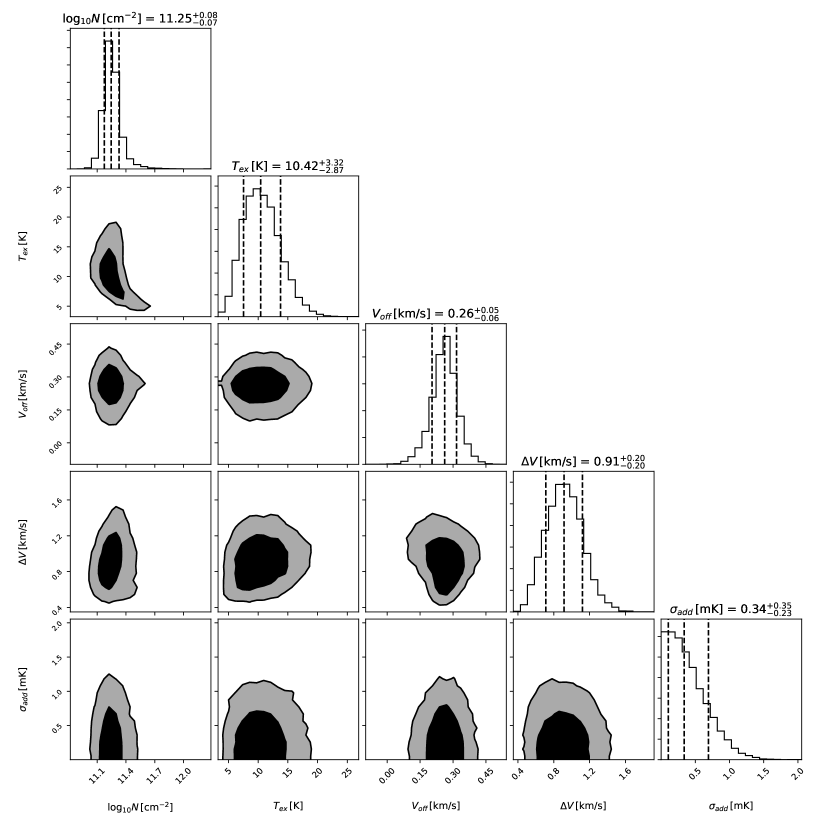
Figure 2: 1D and 2D histograms of the posterior distribution of parameters for HOCO⁺. Contours contain 68 and 95 % of samples, respectively. Uncertainty quoted here are statistical only, without 10% calibration error. $V_{off}$ is the difference between the observed line position and the reference $V_{lsr}$ position for IRAS 16293 of 3.6 km/s ($V_{line}$ = $V_{lsr}$ + $V_{off}$ with $V_{lsr}$=3.8 km/s).

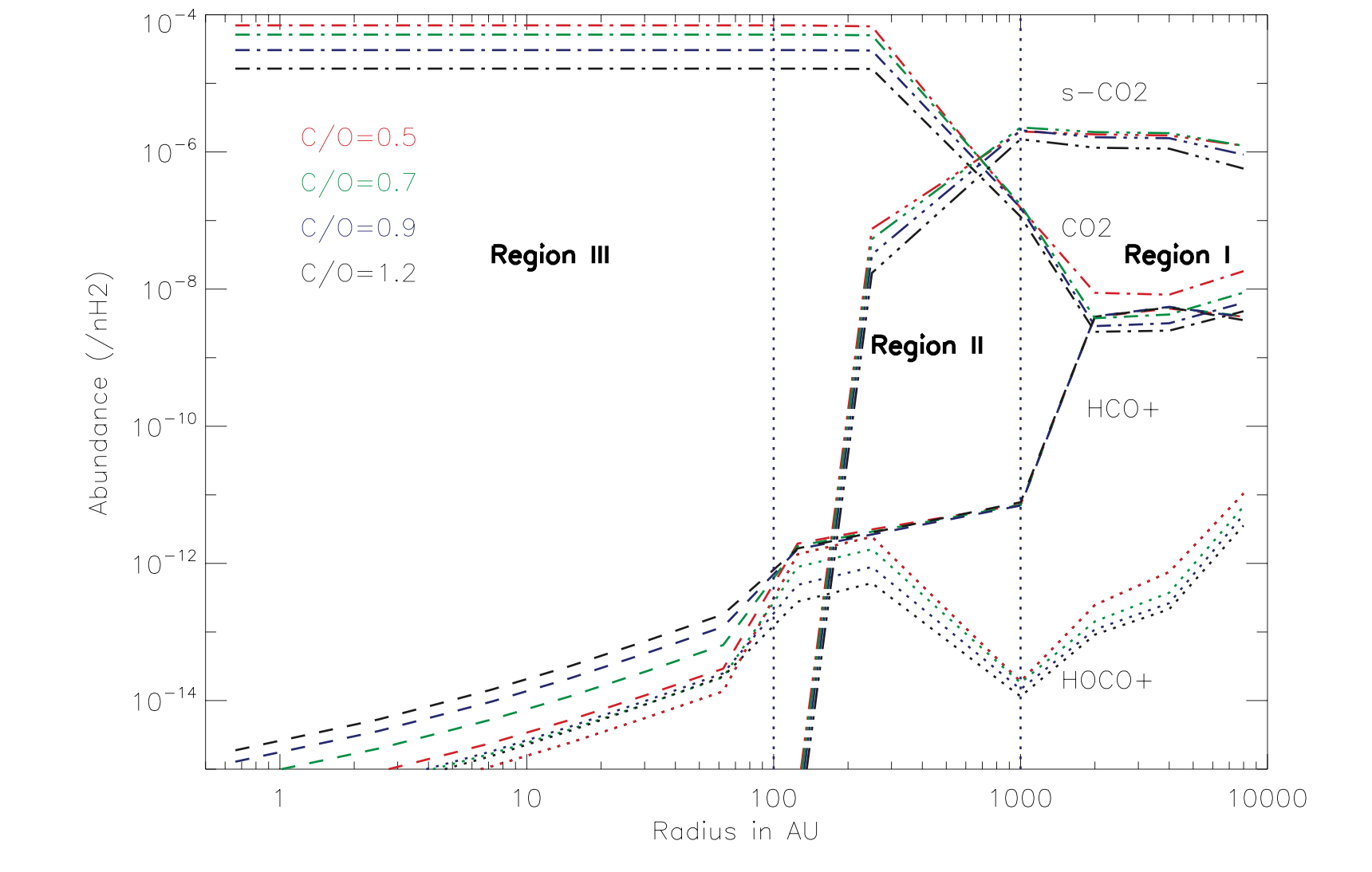
Figure 3: Abundance with respect to H₂ for HOCO⁺, HCO⁺, CO₂ predicted by our model as a function of radius. s-CO₂ represents the CO₂ on the surface of grains.

2.2.2 LTE modelling of HOCO⁺

We have used the bayesian model similar to the one used in Majumdar et al. (2017). They used this model to recover the distribution of parameters which best agree with the observed line intensities of c-C₃H₂ and c-C₃HD in the same source.

In order to model the emission of HOCO⁺, we have used an LTE radiative transfer code based on the equations described in Maret et al. (2011). The model needs the species column density, the line width, the excitation temperature, the source size and an accurate molecular spectroscopic catalog which contains energy levels with associated quantum numbers, statistical weights and transition frequencies as well as integrated intensities at 300 K. For HOCO⁺, we have used the spectroscopic data from Bizzocchi et al. (2017) retrieved from the CDMS database (Müller et al., 2005). All the detected frequencies along with their Einstein coefficients, upper level energies and the associated quantum numbers are listed in Table 1.

Since we have only two detected lines, we have considered a fixed source size of 25 arcsec ($\sim$ 3000 AU, a typical size of the protostellar envelope; Caux et al. (2011)). In our model, the likelihood function assumes that the errors are distributed with a noise term. This noise term is defined as the sum in quadrature of the observed per channel uncertainty and an additional noise term (noted as $\sigma_{add}$ in Figure 2) left as a free parameter in the model. By following Majumdar et al. (2017), here also we have assumed similar distribution of the priors. We carried out sampling of the posterior distribution using the Hamilonian Monte Carlo NUTS sampler implemented in the Stan package and the PyStan wrapper . The sampling was run for 2000 iterations using 6 independent chains, with the 1000 first iterations discarded for warmup. Convergence was checked by computing the split $\hat{R}$ estimator (Gelman & Rubin, 1992) for all parameters, all of which were found to be less than 1.01.

Figure 1 shows the comparison of the observed and modelled spectra for HOCO⁺. In Figure 2, we have shown the 1D and 2D histograms of the posterior probability distribution function for HOCO⁺. From Figure 2, it is very clear that excitation temperature, systematic velocity and line width are well defined. In Table 2, we have summarised the one point statistics for the marginalised posterior distributions of parameters with 1$\sigma$ symmetric error bars in the parentheses. We have used the H₂ column density of 1.6$\times$ 10²⁴ cm^-2 derived by Schöier et al. (2002) in the cold envelope to derive the HOCO⁺ abundance. We have also listed modelled abundance of HOCO⁺ at 3000 AU discussed in the Section 3.

Table 2: Point estimates of the posterior distribution function corresponding to the median and one sigma uncertainty.

Parameter	Value
$\mathrm{\log N(HOCO^{+})}$ ($\mathrm{\,cm^{-2}}$)	$11.25\pm 0.08$
$\mathrm{T_{ex}}$ ($\mathrm{\,K}$)	$10\pm 3$
$\mathrm{\Delta V}$ ($\mathrm{\,km\,s^{-1}}$)	$0.9\pm 0.2$
$\mathrm{\log[HOCO^{+}]^{observation}}$	$-12.95\pm 0.08$
$\mathrm{\log[HOCO^{+}]^{model(C/O=0.5)}}$	-12.32
$\mathrm{\log[HOCO^{+}]^{model(C/O=0.7)}}$	-12.61
$\mathrm{\log[HOCO^{+}]^{model(C/O=0.9)}}$	-12.76
$\mathrm{\log[HOCO^{+}]^{model(C/O=1.2)}}$	-12.85

3 Chemistry of HOCO⁺ in the proto-stellar envelope

3.1 The NAUTILUS chemical model

We have investigated the chemistry of HOCO⁺ in IRAS 16293 by using the state-of-the-art NAUTILUS three phase chemical model (Ruaud et al., 2016). NAUTILUS computes the chemical composition as a function of time in the gas-phase, and at the surface of interstellar grains. All the physicochemical processes included in the model along with their corresponding equations are described in detail in Ruaud et al. (2016). Our gas phase chemistry is based on the public chemical network kida.uva.2014 (Wakelam et al., 2015). The surface network is based on the one of Garrod et al. (2007) with several additional processes from Ruaud et al. (2015). By following Hincelin et al. (2011), we adopt the similar initial elemental abundances with an additional elemental abundance of $6.68\times 10^{-9}$ for fluorine (Neufeld et al. (2005)) and different C/O elemental ratios of 0.5, 0.7, 0.9, 1.2.

3.2 1D physical model

The physical model for IRAS 16293 follows the one detailed in our previous papers (Majumdar et al. (2016); Majumdar et al. (2017)). It was based on the radiation hydrodynamical (RHD) simulations from Masunaga & Inutsuka (2000). This physical dynamical model starts from a dense molecular cloud with a central density $n$(H₂) $\sim 3\times 10^{4}$ cm^-3 and the core extends up to $r=4\times 10^{4}$ AU with a total mass of 3.852 $M_{\odot}$, which exceeds the critical mass for gravitational instability. The initial temperature for the core is around 7 K at the center and around 8 K at the outer edge. In order to set up the initial molecular conditions for the collapse stage, the core stays at its hydrostatic structure for 10⁶ year.

After 10⁶ year, the contraction starts for the core and it is almost isothermal as long as the cooling is efficient. When compressional heating overwhelms the cooling, it causes a rise of the temperature in the central region. Eventually, the first hydrostatic core forms when contraction decelerates due to the increase of the gas pressure. This is also known as ‘first core’ at the center.

A second collapse happens when the core center becomes unstable due to a very high density of 10⁷ cm^-3 and a high temperature of 2000 K which causes H₂ dissociation. Within a short period of time, the dissociation degree approaches unity at the center due to the rapid increase of central density. Then the second collapse ceases, and the second hydrostatic core, i.e., the protostar, is formed and the infalling envelope around this protostar is known as ‘protostellar core’. It takes a $2.5\times 10^{5}$ yr for the initial pre-stellar core to evolve into the protostellar core.

When the protostar is formed, the model again follows the evolution for a $9.3\times 10^{4}$ yr, during which the protostar grows by mass accretion from the envelope.

3.3 Results and discussions

Figure 3 shows the computed abundance of HOCO⁺ in the gas phase in the protostellar envelope as a function of radius to the central protostar, at the end of the simulations (i.e. at the protostellar age of $9.3\times 10^{4}$ yr) for different C/O elemental ratios of 0.5, 0.7, 0.9, 1.2. The “age" that we considered for the protostar is set by the physical dynamical model. As discussed in Wakelam et al. (2014), the physical structure obtained with the radiation hydrodynamical model at that time is similar to the one constrained by multi-wavelength dust and molecular observations (from Crimier et al. (2010)). We have also shown the abundance profile of HCO⁺ and CO₂ as they are the major precursors for the formation of HOCO⁺.

Hincelin et al. (2011) have already performed a detailed sensitivity analysis to the different oxygen elemental abundances. They have concluded that gas phase abundances calculated with the NAUTILUS gas-grain chemical model are less sensitive to the elemental C/O ratio than those computed with a pure gas phase chemical model (Wakelam et al., 2010). This is consistent with our current results shown in Figure 3. The grain surface chemistry plays the role of a buffer absorbing most of the extra carbon. This is fortunate because the C depletion problem is still poorly understood from observations. This reduced sensitivity of the chemistry to the C/O ratio makes this conclusion more robust.

For our discussion, we divide our model into three different regions: (i) a first region (radii larger than 1000 AU and temperatures below 30 K), (ii) a second region (radius in between 1000 and 200 AU and temperature in between 30 and 60 K) (iii) and a third region (radii lower than 200 AU and temperatures higher than 60 K; $\sim$ 70-250 K in between 150 to 10 AU).

In the first region, HOCO⁺ is mainly formed from the OH + HCO⁺ and CO₂ + H₃⁺ reactions. The contribution of OH + HCO⁺$\rightarrow$ H + HOCO⁺ reaction is $\sim$85% towards the HOCO⁺ formation. The contribution of the second reaction is much less since CO₂ is frozen on the grains. In this region, HCO⁺ is the main precursor for HOCO⁺ formation. The HCO⁺ is mainly formed from the CO + H${}_{3}^{+}$ reaction whereas OH radical originates mostly from the dissociative recombination reactions of H₃O⁺. Formation of H₃⁺ and hence HCO⁺ are governed by the reaction with cosmic rays. Thus, in the outer part of the envelope, the HOCO⁺ abundance is controlled by the cosmic rays.

In the second region, HOCO⁺ is mainly formed from the CO₂ + H${}_{3}^{+}$ reaction. The contribution of this reaction is $\sim$85% towards the HOCO⁺ formation. In this region, CO₂ is the major precursor for HOCO⁺ formation since the abundance of gas phase CO₂ starts increasing due to thermal desorption in the inner part of the envelope. A small fraction of HOCO⁺ is also produced from the CO₂ + N₂H⁺ reaction and the efficiency of the OH + HCO⁺ reaction is almost negligible due to the rapid fall in HCO⁺ abundance. Here, HOCO⁺ is destroyed by CO + HOCO⁺$\rightarrow$CO₂ + HCO⁺ and CH₄ + HOCO⁺$\rightarrow$CO₂ + CH₅⁺ reactions. The second HOCO⁺ peak around 200 AU is due to the effect of thermal desorption of the CO₂ ice.

Recently, Vastel et al. (2016) have observed HOCO⁺ in the L1544 prestellar core. The observed abundance was ($5\pm 2)\times 10^{-11}$ with respect to molecular hydrogen. They also performed modeling of HOCO⁺ in this source using a gas phase chemical code. In their model, they used a C/O ratio of 0.5, cosmic ray ionization rate of $3\times 10^{-17}$ s^-1, n(H) equal to $2\times 10^{4}$ cm^-3, a temperature of 10 K and A_v=10 magnitude. Finally, they compared the steady-state abundance of HOCO⁺ which is equal to $4\times 10^{-11}$ with respect to molecular hydrogen with the observed abundance. The main conclusion from their model is that the chemistry of HOCO⁺ depends on the reaction HCO⁺ + OH$\rightarrow$HOCO⁺ + H when CO₂ is frozen on the grains. HOCO⁺ abundance depends on the CO₂ + H${}_{3}^{+}$$\rightarrow$HOCO⁺ + H₂ reaction when gaseous CO₂ abundance is increased due to desorption processes. The major reactions that contributed to forming HOCO⁺ in Vastel et al. (2016) are consistent with our findings. The only exception is cosmic-ray induced UV photo-desorption (Caselli et al., 2012) is likely for CO₂ ice in L1544 as compared to thermal desorption (Vastel et al., 2016).

The HOCO⁺ and CO₂ abundance profile in the gas phase are correlated till 200 AU. In the third region (radii lower than 200 AU), HOCO⁺ and HCO⁺ abundances decrease rapidly due to very efficient destruction channels via H₂O + HOCO⁺$\rightarrow$ CO₂ + H₃O⁺ ($\sim$ 77%), CO + HOCO⁺$\rightarrow$ CO₂ + HCO⁺ ($\sim$ 15%), H₂O + HCO⁺$\rightarrow$ CO + H₃O⁺ ($\sim$ 67%) and HCN + HCO⁺$\rightarrow$ CO + HCNH⁺ ($\sim$ 18%) reactions. Due to close interplay of these four reactions, the abundance of HOCO⁺ is correlated with that of HCO⁺ in the inner part of the envelope.

The abundances of HOCO⁺ predicted by our model at 3000 AU (approximate size of the envelope) are $4.7\times 10^{-13}$, $2.4\times 10^{-13}$, $1.7\times 10^{-13}$ and $1.4\times 10^{-13}$ with respect to molecular hydrogen for C/O ratios of 0.5, 0.7, 0.9 and 1.2 respectively. Looking at the small differences between these chemical models with different C/O ratios, we think HOCO⁺ is not a good tracer to constrain the elemental C/O ratios in IRAS 16293. The observed abundance of HOCO⁺ is ($1.12\pm 0.3)\times 10^{-13}$ with respect to molecular hydrogen (See Table 2). We have used the H₂ column density of 1.6$\times$ 10²⁴ cm^-2 from Schöier et al. (2002) which corresponds to the full line of sight including the hot corino whereas HOCO⁺ was assumed to be coming from the envelope. Therefore the derived observed abundance is most probably a lower limit to the abundance in the outer envelope. Schöier et al. (2002) have also derived the abundance of HCO⁺ in the cold envelope by assuming the same H₂ column density of 1.6$\times$ 10²⁴ cm^-2 and the derived value was $1.4\times 10^{-09}$ with respect to molecular hydrogen. We compare the abundance ratios of [HOCO⁺] to [HCO⁺] which yield a value of 8$\times$ 10^-5 from the observation. This value is reasonably close to the ratio 5$\times$$10^{-5}$ from our model (by considering [HOCO⁺]$\sim$ $2.4\times 10^{-13}$ and [HCO⁺]$\sim$ $4.8\times 10^{-09}$ for a standard C/O ratio of 0.7 (Hincelin et al., 2011) used generally in our models). Vastel et al. (2016) have derived [HOCO⁺] to [HCO⁺] ratio in L1544 by assuming the bulk of the emission arrises from the outer layer. The derived value was 6.2$\times$$10^{-3}$ by considering an H₂ column density of 5$\times$ 10²¹ cm^-2. Comparative studies with higher spatial resolution using ALMA/NOEMA interferometers may help us to understand the underlying physics and chemistry better.

At 3000 AU, the abundance of CO₂ in the ice phase is $2\times 10^{-6}$ with respect to molecular hydrogen. Higher abundance of CO₂ ice in the protostellar envelope shows that the JWST-MIRI and NIRSpec will be able to give a wealth of information on the chemistry of CO₂ formation on molecular ices. With James Webb Space Telescope (JWST), scheduled to be launched in 2019, the spectroscopy of molecular ices could be done in the 0.6 to 28.5 micron wavelength range. It is approximately 100 times more powerful than Hubble and Spitzer space telescopes. It has greater sensitivity, higher spatial resolution in the infrared and significantly higher spectral resolution in the mid infrared. CO₂ ice has two strong vibrational modes; the asymmetric stretching mode centered on 4.27 micron, and the bending mode at 15.2 micron, accessible via JWST NIRSpec (0.6-5 micron with single slit spectroscopy mode) and MIRI (11.9-18 micron with IFU mode). These infrared vibrational features are sensitive to the astrophysical environments and band profiles can guide astronomers whether CO₂ molecules are embedded in H₂O, CO ices or other CO₂ isotopes (Bosman et al., 2017). Detection of HOCO⁺ in the solar type protostar IRAS 16293 will motivate future observation of CO₂ (which is one of the important constituent of planetary atmospheres) in similar type of environments using JWST.

References

- Aikawa et al. (2012) Aikawa Y., et al., 2012, A&A, 538, A57
- Bergin et al. (2005) Bergin E. A., Melnick G. J., Gerakines P. A., Neufeld D. A., Whittet D. C. B., 2005, ApJ, 627, L33
- Bizzocchi et al. (2017) Bizzocchi L., et al., 2017, A&A, 602, A34
- Boogert et al. (2004) Boogert A. C. A., et al., 2004, ApJS, 154, 359
- Boonman et al. (2003) Boonman A. M. S., van Dishoeck E. F., Lahuis F., Doty S. D., 2003, A&A, 399, 1063
- Bosman et al. (2017) Bosman A. D., Bruderer S., van Dishoeck E. F., 2017, A&A, 601, A36
- Caselli et al. (2012) Caselli P., et al., 2012, ApJ, 759, L37
- Caux et al. (2011) Caux E., et al., 2011, A&A, 532, A23
- Cooke et al. (2016) Cooke I. R., Fayolle E. C., Öberg K. I., 2016, ApJ, 832, 5
- Crimier et al. (2010) Crimier N., Ceccarelli C., Maret S., Bottinelli S., Caux E., Kahane C., Lis D. C., Olofsson J., 2010, A&A, 519, A65
- D’Hendecourt et al. (1985) D’Hendecourt L. B., Allamandola L. J., Greenberg J. M., 1985, A&A, 152, 130
- D’Hendecourt et al. (1986) D’Hendecourt L. B., Allamandola L. J., Grim R. J. A., Greenberg J. M., 1986, A&A, 158, 119
- Garrod et al. (2007) Garrod R. T., Wakelam V., Herbst E., 2007, A&A, 467, 1103
- Gelman & Rubin (1992) Gelman A., Rubin D., 1992, Statistical Science, 7, 457
- Gerakines et al. (1999) Gerakines P. A., et al., 1999, ApJ, 522, 357
- Herbst & Leung (1989) Herbst E., Leung C. M., 1989, ApJS, 69, 271
- Herbst et al. (1977) Herbst E., Green S., Thaddeus P., Klemperer W., 1977, ApJ, 215, 503
- Hincelin et al. (2011) Hincelin U., Wakelam V., Hersant F., Guilloteau S., Loison J. C., Honvault P., Troe J., 2011, A&A, 530, A61
- Jiménez-Serra et al. (2016) Jiménez-Serra I., et al., 2016, ApJ, 830, L6
- Knez et al. (2005) Knez C., et al., 2005, ApJ, 635, L145
- Majumdar et al. (2016) Majumdar L., Gratier P., Vidal T., Wakelam V., Loison J.-C., Hickson K. M., Caux E., 2016, MNRAS, 458, 1859
- Majumdar et al. (2017) Majumdar L., Gratier P., Andron I., Wakelam V., Caux E., 2017, MNRAS, 467, 3525
- Majumdar et al. (2018) Majumdar L., Loison J.-C., Ruaud M., Gratier P., Wakelam V., Coutens A., 2018, MNRAS, 473, L59
- Maret et al. (2011) Maret S., Hily-Blant P., Pety J., Bardeau S., Reynier E., 2011, A&A, 526, A47
- Masunaga & Inutsuka (2000) Masunaga H., Inutsuka S.-i., 2000, ApJ, 531, 350
- Millar et al. (1991) Millar T. J., Bennett A., Rawlings J. M. C., Brown P. D., Charnley S. B., 1991, A&AS, 87, 585
- Minh et al. (1991) Minh Y. C., Brewer M. K., Irvine W. M., Friberg P., Johansson L. E. B., 1991, A&A, 244, 470
- Müller et al. (2005) Müller H. S. P., Schlöder F., Stutzki J., Winnewisser G., 2005, Journal of Molecular Structure, 742, 215
- Neufeld et al. (2005) Neufeld D. A., Wolfire M. G., Schilke P., 2005, ApJ, 628, 260
- Noble et al. (2013) Noble J. A., Fraser H. J., Aikawa Y., Pontoppidan K. M., Sakon I., 2013, ApJ, 775, 85
- Öberg et al. (2011) Öberg K. I., Boogert A. C. A., Pontoppidan K. M., van den Broek S., van Dishoeck E. F., Bottinelli S., Blake G. A., Evans II N. J., 2011, ApJ, 740, 109
- Ootsubo et al. (2012) Ootsubo T., et al., 2012, ApJ, 752, 15
- Podio et al. (2014) Podio L., Lefloch B., Ceccarelli C., Codella C., Bachiller R., 2014, A&A, 565, A64
- Pontoppidan et al. (2008) Pontoppidan K. M., et al., 2008, ApJ, 678, 1005
- Roser et al. (2001) Roser J. E., Vidali G., Manicò G., Pirronello V., 2001, ApJ, 555, L61
- Ruaud et al. (2015) Ruaud M., Loison J. C., Hickson K. M., Gratier P., Hersant F., Wakelam V., 2015, MNRAS, 447, 4004
- Ruaud et al. (2016) Ruaud M., Wakelam V., Hersant F., 2016, MNRAS, 459, 3756
- Sakai et al. (2008) Sakai N., Sakai T., Aikawa Y., Yamamoto S., 2008, ApJ, 675, L89
- Schöier et al. (2002) Schöier F. L., Jørgensen J. K., van Dishoeck E. F., Blake G. A., 2002, A&A, 390, 1001
- Shimonishi et al. (2010) Shimonishi T., Onaka T., Kato D., Sakon I., Ita Y., Kawamura A., Kaneda H., 2010, A&A, 514, A12
- Thaddeus et al. (1981) Thaddeus P., Guelin M., Linke R. A., 1981, ApJ, 246, L41
- Vastel et al. (2016) Vastel C., Ceccarelli C., Lefloch B., Bachiller R., 2016, A&A, 591, L2
- Vasyunin et al. (2017) Vasyunin A. I., Caselli P., Dulieu F., Jiménez-Serra I., 2017, ApJ, 842, 33
- Wakelam et al. (2010) Wakelam V., Herbst E., Le Bourlot J., Hersant F., Selsis F., Guilloteau S., 2010, A&A, 517, A21
- Wakelam et al. (2014) Wakelam V., Vastel C., Aikawa Y., Coutens A., Bottinelli S., Caux E., 2014, MNRAS, 445, 2854
- Wakelam et al. (2015) Wakelam V., et al., 2015, ApJS, 217, 20
- Whittet et al. (1998) Whittet D. C. B., et al., 1998, ApJ, 498, L159
- Whittet et al. (2009) Whittet D. C. B., Cook A. M., Chiar J. E., Pendleton Y. J., Shenoy S. S., Gerakines P. A., 2009, ApJ, 695, 94
- van Dishoeck et al. (1996) van Dishoeck E. F., et al., 1996, A&A, 315, L349