Current-induced forces for nonadiabatic molecular dynamics

Abstract

We present general first principles derivation of expression for current-induced forces. The expression is applicable in non-equilibrium molecular systems with arbitrary intra-molecular interactions and for any electron-nuclei coupling. It provides a controlled consistent way to account for quantum effects of nuclear motion, accounts for electronic non-Markov character of the friction tensor, and opens way to treatments beyond strictly adiabatic approximation. We show connection of the expression with previous studies, and discuss effective ways to evaluate the friction tensor.

Introduction. Nonadiabatic molecular dynamics (NAMD) is a fundamental problem related to breakdown of the usual timescale separation (the Born-Oppenheimer approximation) between electron and nuclear dynamics. The NAMD plays an important role in many processes, ranging from chemistry Jiang et al. (2016); Ouyang et al. (2015) and photochemistry Lei et al. (2016) to spectroscopy Bennett et al. (2016); Petit and Subotnik (2015); Petit and Subotnik (2014a, b) and nonradiative electronic relaxation Long et al. (2016), and from electron and proton transfer Wang et al. (2015); Xu et al. (2016); Liu et al. (2016) to coherent control Tiwari and Henriksen (2016) and photo-induced energy transfer Lee et al. (2016); Krüger et al. (2015). Significance of the problem stems from both complexity of it fundamental theoretical description, and applicational importance for development of optoelectronic Ohmura et al. (2016); Nelson et al. (2014) and optomechanical Nikiforov et al. (2016) molecular devices.

A crucial part of formulating nuclear dynamics is definition of nuclear forces induced by electronic subsystem. A number of recent studies has discussed ways to account for “electronic friction” in the dynamics Bode et al. (2011, 2012); Shenvi and Tully (2012); Falk et al. (2014); Dou et al. (2015); Askerka et al. (2016); Maurer et al. (2016); Dou and Subotnik (2016); Dou et al. (2017); Dou and Subotnik (2017). Majority of the studies employ intuitive reasoning in the formulations Shenvi and Tully (2012); Falk et al. (2014); Dou et al. (2015); Askerka et al. (2016); Maurer et al. (2016); Dou and Subotnik (2016); Dou et al. (2017); Dou and Subotnik (2017). Also, some of the works are confined only to non-interacting and/or equilibrium electronic systems Shenvi and Tully (2012); Falk et al. (2014); Dou et al. (2015); Askerka et al. (2016); Maurer et al. (2016); Dou and Subotnik (2016, 2017). A consistent derivation of nuclear forces was presented within path integral formulation employing the Feynman-Vernon influence functional Brandbyge et al. (1995); Lü et al. (2012, 2015). The derivation lead to Langevin equation driven by a set of forces: friction, non-conservative, renormalization, and Berry phase. However, the studies are restricted to non-interacting electronic systems and to linear coupling between nuclear and electronic degrees of freedom Lü et al. (2012, 2015). Finally, all the aforementioned works consider only extremely slow (Ehrenfest) nuclear dynamics.

Here we discuss a derivation of nuclear forces for nonadiabatic nuclear dynamics, which accounts for nonequilibrium character of a molecular system, intra-molecular interactions, and general coupling between electronic and nuclear degrees of freedom. Moreover, the consideration goes beyond extremely slow (Ehrenfest) limit of nuclear motion; so that resulting expressions are valid also in the intermediate regime and are applicable in surface hopping considerations. Structure of the paper is as follows: first weintroduce a model and present the general derivation. After that, we show relation to previous studies indicating corresponding approximations, establish connection with the Zubarev’s method of nonequilibrium statistical operator, and discuss efficient ways to simulate the forces in nonequilibrium interacting molecular systems. Finally, we summarize our findings and indicate directions of further research.

General derivation. We consider dynamics of a molecule $M$ adsorbed on a surface(s) $K$. Hamiltonian of the system is separated into nuclear kinetic and potential energies, and electron Hamiltonian which depends on nuclear coordinates $\hat{q}$

$$\hat{H}=\sum_{\alpha}\frac{\hat{p}_{\alpha}^{2}}{2}+\hat{V}(\hat{q})+\hat{H}_{e}(\hat{q})$$ (1)

$\hat{H}_{e}(\hat{q})$ consists of molecular $\hat{H}_{M}(\hat{q})$ and contacts $\hat{H}_{K}$ parts, and coupling $\hat{V}_{K}(\hat{q})$ between them. $\hat{H}_{M}(\hat{q})$ can include any intra-molecular interactions and is represented in the basis of many-body electronic states $\{\lvert S\rangle\}$. Explicit expressions are

$$\hat{H}_{M}=\sum_{S_{1},S_{2}}\lvert S_{1}\rangle H^{e}_{S_{1}S_{2}}(\hat{q})\langle S_{2}\rvert;\quad\hat{H}_{K}=\sum_{k\in K}\varepsilon_{k}\,\hat{c}_{k}^{\dagger}\hat{c}_{k};$$ (2)

$$\hat{V}_{K}=\sum_{k\in K}\sum_{(S_{1},S_{2})}\bigg{(}V_{k\,(S_{1},S_{2})}(\hat{q})\,\hat{c}_{k}^{\dagger}\,\lvert S_{1}\rangle\langle S_{2}\rvert+H.c.\bigg{)}$$

Here $\hat{c}_{k}^{\dagger}$ ($\hat{c}_{k}$) creates (annihilates) electron in state $k$ of contact $K$, $S_{1}$ and $S_{2}$ indicate a pair of molecular many-body states which belong to the same charging block ($N_{S_{1}}=N_{S_{2}}$) in $\hat{H}_{M}$ and to charging blocks different by one electron ($N_{S_{1}}+1=N_{S_{2}}$) in $\hat{V}_{K}$ ($N_{S}$ is number of electrons in state $\lvert S\rangle$). Note that although $\hat{H}_{M}$ is written in the diabatic basis, derivation below is not restricted to this particular choice.

Effective evolution for the nuclear density matrix is obtained by tracing density matrix of the whole system over electron degrees of freedom $\hat{\rho}_{vib}\equiv\mbox{Tr}_{e}\{\hat{\rho}\}$. Assuming initial density matrix being direct product of nuclear and electron density matrices, $\hat{\rho}^{(0)}=\hat{\rho}_{vib}^{(0)}\otimes\hat{\rho}_{el}^{(0)}$, nuclear effective evolution can be represented in terms of the Feynman-Vernon functional $F$ Feynman and Vernon (1963)

$$\rho_{vib}(2)=\int d1\,\mathcal{K}(2;1)\,\rho_{vib}(1)$$ (3)

$$\mathcal{K}(2;1)=\int_{1}^{2}D(x,y)\,e^{i\big{(}S_{vib}(x)-S_{vib}(y)\big{)}}\,F(x,y)$$ (4)

$$S_{vib}(q)=\int dt\,L(q,\dot{q})\equiv\int dt\bigg{(}\sum_{\alpha}\frac{\dot{q}_{\alpha}^{2}}{2}-V(q)\bigg{)}$$ (5)

$$F(x,y)=\bigg{\langle}T_{c}\,e^{-i\int_{c}d\tau\,\hat{H}_{e}\big{(}q(\tau)\big{)}}\bigg{\rangle}\equiv e^{{}\,i\,S_{eff}(x,y)}$$ (6)

Here $i\equiv(x,y)$ ($i=1,2$) represent pair of nuclear coordinates on time-ordered, $x$, and anti-time-ordered, $y$, branches of the Keldysh contour, $\mathcal{K}(2,1)$ is the nuclear propagation kernel from time $t_{1}$ to $t_{2}$, $S_{vib}(q)$ ($q=x,y$) is the action of free nuclear evolution, $T_{c}$ is the contour ordering operator, and $\langle\ldots\rangle$ is quantum mechanical and statistical average over only electronic degrees of freedom.

Now we want to derive expression for the effective action $S_{eff}$, Eq. (6). To do so we separate classical, $Q_{\alpha}$, and quantum, $\xi_{\alpha}$, nuclear dynamics by transferring to the Wigner coordinates

$$Q_{\alpha}=\frac{x_{\alpha}+y_{\alpha}}{2}\qquad\xi_{\alpha}=x_{\alpha}-y_{\alpha}$$ (7)

and rewrite the Hamiltonian in the form of zero-order classical nuclear evolution plus quantum perturbation

$$\hat{H}_{e}\big{(}q(\tau)\big{)}=\hat{H}_{e}\big{(}Q(\tau)\big{)}+\hat{V}_{e}\big{(}q(\tau)\big{)}$$ (8)

where $\hat{V}_{e}\big{(}q(\tau)\big{)}\equiv\hat{H}_{e}\big{(}q(\tau)\big{)}-\hat{H}_{e}\big{(}Q(\tau)\big{)}$. Following Ref. Brandbyge et al., 1995 we replace $\hat{V}_{e}\big{(}q(\tau)\big{)}$ by $\lambda\hat{V}_{e}\big{(}q(\tau)\big{)}$, and employ the linked cluster theorem. This leads to

$$S_{eff}(x,y)=-\int_{0}^{1}d\lambda\int_{c}d\tau\big{\langle}\hat{V}_{e}^{H}\big{(}q(\tau)\big{)}\big{\rangle}_{c}$$ (9)

Here superscript $H$ shows that the operator is in the Heisenberg picture, and subscript $c$ indicates that one has to consider only connected diagrams.

So far consideration is exact. Now we perform expansion of (9) in $\lambda\hat{V}_{e}\big{(}q(\tau)\big{)}$. We justify the expansion in ‘quantumness’ of the nuclei by noting that for purely classical nuclei, $x=y$, the functional (6) is unity Kamenev (2011) and that for relatively slow nuclear motion deviation from classical trajectory is small. Expanding (9) up to first order in $\lambda\hat{V}_{e}\big{(}q(\tau)\big{)}$ and evaluating integrals in $\lambda$ yields

$$S_{eff}(x,y)\approx -\bigg{\langle}\int_{c}d\tau\,\hat{V}_{e}^{I}\big{(}q(\tau)\big{)}\bigg{\rangle}_{c}$$ (10)

$$+ \frac{i}{2}\bigg{\langle}T_{c}\,\int_{c}d\tau_{1}\int_{c}d\tau_{2}\,\hat{V}_{e}^{I}\big{(}q(\tau_{1})\big{)}\,\hat{V}_{e}^{I}\big{(}q(\tau_{2})\big{)}\bigg{\rangle}_{c}$$

where superscript $I$ shows that the operator is in the interaction picture, i.e. its evolution is defined by Hamiltonian $\hat{H}_{e}\big{(}Q(\tau)\big{)}$. Here, first row corresponds to first order and second - to second order of the cumulant expansion. Employing the Langreth rules Haug and Jauho (2008) to project (10) onto real time axis and expanding $\hat{V}_{e}\big{(}q(\tau)\big{)}$ up to second order in the quantum coordinates $\xi_{\alpha}$ leads to

$$S_{eff}(x,y) \approx-\sum_{\alpha}\int dt\;\xi_{\alpha}(t)\,\big{\langle}\partial_{\alpha}\hat{H}_{e}^{I}\big{(}Q(t)\big{)}\big{\rangle}_{c}$$ (11)

$$+\frac{i}{2}\sum_{\alpha,\beta}\int dt_{1}\int dt_{2}\,\xi_{\alpha}(t_{1})\,\Pi_{\alpha\beta}(t_{1},t_{2})\,\xi_{\beta}(t_{2})$$

where

$$\big{\langle}\partial_{\alpha}\hat{H}_{e}^{I}\big{(}Q(t)\big{)}\big{\rangle}_{c}\equiv\mbox{Tr}_{e}\big{\{}\partial_{\alpha}\hat{H}_{e}\big{(}Q(t)\big{)}\,\hat{\rho}_{el}(t)\big{\}}_{c}$$ (12)

$$\Pi_{\alpha\beta}(t_{1},t_{2})=\frac{1}{2}\bigg{\langle}\bigg{\{}\partial_{\alpha}\hat{H}_{e}^{I}\big{(}Q(t_{1})\big{)};\partial_{\beta}\hat{H}_{e}^{I}\big{(}Q(t_{2})\big{)}\bigg{\}}\bigg{\rangle}_{c}$$ (13)

Here $\{\ldots;\ldots\}$ is anti-commutator and $\hat{H}_{e}\big{(}Q(t)\big{)}$ is the electronic Hamiltonian in the Schrödinger picture build for nuclear frame $Q(t)$.

Using (11) in (4) yields

$$\mathcal{K}(2;1)=\int D(Q,\xi)\exp\bigg{[}i\xi_{2}\dot{Q}_{2}-i\xi_{1}\dot{Q}_{1}\bigg{]}\times$$ (14)

$$\exp\bigg{[}i\sum_{\alpha}\int dt\,\xi_{\alpha}(t)\bigg{(}L_{\alpha}(t)+i\sum_{\beta}\int dt^{\prime}\,\Pi_{\alpha\beta}(t,t^{\prime})\frac{\xi_{\beta}(t^{\prime})}{2}\bigg{)}\bigg{]}$$

where

$$L_{\alpha}(t)=-\ddot{Q}_{\alpha}(t)-\partial_{\alpha}V\big{(}Q(t)\big{)}-\big{\langle}\partial_{\alpha}\hat{H}_{e}^{I}\big{(}Q(t)\big{)}\big{\rangle}$$ (15)

is the Lagrangian. Finally, employing the Hubbard-Stratonovich transformation and integrating out the quantum coordinates leads to

$$\ddot{Q}_{\alpha}(t)=-\partial_{\alpha}V\big{(}Q(t)\big{)}-\big{\langle}\partial_{\alpha}\hat{H}_{e}^{I}\big{(}Q(t)\big{)}\big{\rangle}+f_{\alpha}(t)$$ (16)

where $f_{\alpha}(t)$ is stochastic force which satisfies

$$\big{\langle}f_{\alpha}(t_{1})\,f_{\beta}(t_{2})\big{\rangle}=\Pi_{\alpha\beta}(t_{1},t_{2})$$ (17)

Eq. (16) is the stochastic Langevin equation for classical nuclear dynamics driven by quantum electronic bath. The latter is characterized by Eqs. (12), (13), and (17).

Friction tensor. Eq. (16) is starting point of current-induced nuclear forces consideration in Ref. Bode et al., 2012. The consideration was restricted to non-interacting electron systems.

To compare with other results presented in the literature recently, we utilize assumption of fast electron dynamics on the timescale of nuclear motion, which allows to transfer to the reduced description of the nonequilibrium electronic system. In particular, employing Zubarev’s method of the nonequilibrium statistical operator, electronic density operator $\hat{\rho}_{el}(t)$ is expressed in terms of the relevant distribution $\hat{\rho}_{rel}(t)$ as Zubarev et al. (1996)

$$\hat{\rho}_{el}(t)= \hat{\rho}_{rel}(t)-\int_{-\infty}^{t}dt^{\prime}\,e^{-\delta(t-t^{\prime})}\hat{U}(t,t^{\prime})$$ (18)

$$\times \big{\{}\partial_{t^{\prime}}\hat{\rho}_{rel}(t^{\prime})+i\big{[}\hat{H}_{e}\big{(}Q(t^{\prime})\big{)};\hat{\rho}_{rel}(t^{\prime})\big{]}\big{\}}\hat{U}^{\dagger}(t,t^{\prime})$$

where $\hat{U}(t_{1},t_{2})=T\exp\bigg{[}-i\int_{t_{1}}^{t_{2}}dt\,\hat{H}_{e}\big{(}Q(t)\big{)}\bigg{]}$ is the electronic evolution operator under classical nuclear driving, $T$ is time-ordering operator and $\delta\to+0$.

In the limit of extremely slow nuclear driving, when the relevant distribution becomes identical with steady-state electron distribution, $\hat{\rho}_{rel}(t^{\prime})\approx\hat{\rho}_{ss}^{t^{\prime}}$ ($\rho_{ss}^{t^{\prime}}$ is steady-state electronic distribution for nuclear frame $Q(t^{\prime})$) Morozov and Röpke (1998), so that $\big{[}\hat{H}_{e}\big{(}Q(t^{\prime})\big{)};\hat{\rho}_{rel}(t^{\prime})\big{]}\approx 0$ and $\partial_{t^{\prime}}\hat{\rho}_{rel}(t^{\prime})\approx\sum_{\beta}\partial_{\beta}\hat{\rho}_{ss}^{t^{\prime}}\,\dot{Q}_{\beta}(t^{\prime})$, using (18) in (12) yields the Langevin equation (16) in the form

$$\ddot{Q}_{\alpha}(t)= -\partial_{\alpha}V_{eff}\big{(}Q(t)\big{)}$$ (19)

$$-\sum_{\beta}\int dt^{\prime}\,\gamma_{\alpha\beta}(t,t^{\prime})\,\dot{Q}_{\beta}(t^{\prime})+f_{\alpha}(t)$$

Here

$$\partial_{\alpha}V_{eff}\big{(}Q(t)\big{)}\equiv\partial_{\alpha}V\big{(}Q(t)\big{)}+\mbox{Tr}_{e}\big{\{}\partial_{\alpha}\hat{H}_{e}\big{(}Q(t)\big{)}\,\hat{\rho}_{ss}^{t}\big{\}}$$ (20)

$$\gamma_{\alpha\beta}(t_{1},t_{2})\equiv-\theta(t_{1}-t_{2})\,e^{-\delta(t_{1}-t_{2})}$$ (21)

$$\qquad\times\mbox{Tr}_{e}\big{\{}\partial_{\alpha}\hat{H}_{e}\big{(}Q(t_{1})\big{)}\,\hat{U}(t_{1},t_{2})\,\partial_{\beta}\hat{\rho}_{ss}^{t_{2}}\,\hat{U}^{\dagger}(t_{1},t_{2})\big{\}}_{c}$$

are the effective (renormalized) nuclear force and the friction tensor, respectively. Note that Markov version of equation (19) was considered in Refs. Dou et al., 2017; Dou and Subotnik, 2017.

Fluctuation-dissipation theorem. At equilibrium, when nuclei do not move at the timescale of electron correlation, $\hat{\rho}_{ss}\to\hat{\rho}_{eq}=e^{-\beta\hat{H}_{e}(Q)}/Z$, where $\beta=1/k_{B}T$ and $Z=\mbox{Tr}_{e}\big{\{}e^{-\beta\hat{H}_{e}(Q)}\big{\}}$. Employing the Sneddon’s formula Puri (2001), Eq.(21) becomes

$$\gamma_{\alpha\beta}(t_{1}-t_{2})$$ (22)

$$=\beta\,\theta(t_{1}-t_{2})\int_{0}^{1}dx\,\big{\langle}\partial_{\alpha}\hat{H}_{e}^{I}(t_{1})\;\partial_{\beta}\hat{H}_{e}^{I}(t_{2}+i\beta\hbar x)\big{\rangle}_{c}$$

$$=\beta\,\theta(t_{1}-t_{2})\int_{0}^{1}dx\,\big{\langle}\partial_{\beta}\hat{H}_{e}^{I}(t_{2}-i\beta\hbar x)\;\partial_{\alpha}\hat{H}_{e}^{I}(t_{1})\big{\rangle}_{c}$$

This form of $\gamma_{\alpha\beta}$ satisfies the fluctuation-dissipation theorem Zubarev et al. (1996) (see SM Chen et al. (2018) for derivation)

$$\Pi_{\alpha\beta}(E)=E\,\mbox{Re}\,\gamma_{\alpha\beta}(E)\,\coth\frac{\beta E}{2},$$ (23)

which at high temperatures reduces to its classical version $\Pi_{\alpha\beta}(E)=\frac{2}{\beta}\,\mbox{Re}\,\gamma_{\alpha\beta}(E)$. Here $\Pi_{\alpha\beta}(E)$ is the Fourier transform of (13).

Additive electronic Hamiltonian. A number of studies Brandbyge et al. (1995); Bode et al. (2011, 2012); Lü et al. (2012) considered electronic Hamiltonian (2) consisting of zero-order coordinate-independent part and electron-nuclear coupling depending on nuclear coordinates

$$\hat{H}_{e}(\hat{q})=\hat{H}_{e}^{(0)}+\hat{H}_{e}^{(1)}(\hat{q})$$ (24)

In this case, we can expand evolution operator $\hat{U}$ up to linear order in $\hat{H}_{e}^{(1)}$ as $\hat{U}(t_{1},t_{2})\approx\hat{U}_{0}(t_{1},t_{2})-i\int_{t_{2}}^{t_{1}}dt^{\prime}\,\hat{U}_{0}(t_{1},t^{\prime})\,\hat{H}_{e}^{(1)}\big{(}Q(t^{\prime})\big{)}\,\hat{U}_{0}(t^{\prime},t_{2})$, where $\hat{U}_{0}(t_{1},t_{2})=\exp\big{[}-i\,\hat{H}_{e}^{(0)}(t_{1}-t_{2})\big{]}$. Substituting the expansion into (12) and keeping only terms up to second order in $\hat{H}_{e}^{(1)}$ leads to

$$\big{\langle}\partial_{\alpha}\hat{H}_{e}^{I}\big{(}Q(t)\big{)}\big{\rangle}_{c}\approx\big{\langle}\partial_{\alpha}\hat{H}_{e}^{(1)I}\big{(}Q(t)\big{)}\big{\rangle}+\int dt^{\prime}\,\Pi^{r}_{\alpha}(t,t^{\prime})$$ (25)

$$\Pi^{r}_{\alpha}(t,t^{\prime})\equiv-i\,\theta(t-t^{\prime})\big{\langle}\big{[}\partial_{\alpha}\hat{H}_{e}^{(1)I}\big{(}Q(t)\big{)};\hat{H}_{e}^{(1)I}\big{(}Q(t^{\prime})\big{)}\big{]}\big{\rangle}_{c}$$ (26)

Here superscript $I$ indicates interaction picture with respect to Hamiltonian $\hat{H}_{e}^{(0)}$. As previously, first term on the right in (25) renormalizes nuclear potential, while second term accounts for electronic friction. Utilizing second order expansion in $H_{e}^{(1)}$ also in (13) (i.e. using $\hat{U}_{0}$ in place of $\hat{U}$ in the expression) generalizes non-interacting considerations of Refs. Brandbyge et al., 1995; Bode et al., 2011, 2012; Lü et al., 2012 to the case of interacting non-equilibrium systems. As an example in SM Chen et al. (2018) we use (13) and (26) to derive results of Ref. Lü et al. (2012).

Previously introduced in the literature standard friction, nonconservative, renormalization and Berry phase forces are related to our electronic friction as follows. Expressions for the friction, Eqs. (12), (21), or (26), have generic form $F(t,t^{\prime})=\theta(t-t^{\prime})f(t,t^{\prime})$. At steady state, when $f(t,t^{\prime})=f(t-t^{\prime})$, Fourier transform of $F(t,t^{\prime})$ is

$$F(E)=-i\,PP\int\frac{d\omega}{2\pi}\frac{f(\omega)}{E-\omega}+\pi f(E)$$ (27)

where $PP$ is the principle part. The standard friction is identified with $\pi\,\mbox{Im}\,f(E)$, the nonconservative force is given by $\pi\,\mbox{Re}\,f(E)$, the renormalization contribution comes from $PP\int\frac{d\omega}{2\pi}\frac{\mbox{Im}\,f(\omega)}{E-\omega}$, and the Berry phase force is associated with $PP\int\frac{d\omega}{2\pi}\frac{\mbox{Re}\,f(\omega)}{E-\omega}$ (see Ref. Lü et al., 2012 for details).

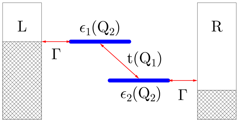
Figure 1: Two-sites two-modes non-interacting junction model of Ref. Lü et al. (2012).

Effective evaluation of the friction tensor. We now discuss effective ways to evaluate current-induced forces in interacting molecular junctions. As discussed in our previous publications White et al. (2014); Galperin and Nitzan (2015); Galperin (2017), methods of the non-equilibrium atomic limit (formulated in the basis of many-body states of the molecule) may be a convenient alternative to standard (orbital based) treatment of electronic degrees of freedom. In particular, recently introduced by us non-equilibrium diagrammatic technique for the Hubbard Green functions Chen et al. (2017); Miwa et al. (2017) may be beneficial also for evaluation of the friction tensor.

Deferring study of non-adiabatic effects on the timescale of electronic correlations to future research, we focus on the additive electronic Hamiltonian (24) with nuclear coordinate dependence confined only to molecular Hamiltonian $\hat{H}_{M}$. In this case the dissipation term, Eq. (26), is

$$\Pi^{r}_{\alpha}(t_{1},t_{2})= \sum_{S_{1},S_{2},S_{3},S_{4}}\partial_{\alpha}H^{e}_{S_{1}S_{2}}(Q)\;H^{e}_{S_{4}S_{3}}(Q)\,$$ (28)

$$\qquad\qquad\times\mathcal{D}^{r}_{S_{1}S_{2},S_{3}S_{4}}(t_{1},t_{2})$$

where $\mathcal{D}^{r}$ is the retarded projection of the single-particle Hubbard Green function

$$\mathcal{D}_{S_{1}S_{2},S_{3}S_{4}}(\tau_{1},\tau_{2})=-i\big{\langle}T_{c}\,\hat{X}_{S_{1}S_{2}}(\tau_{1})\,\hat{X}_{S_{3}S_{4}}^{\dagger}(\tau_{2})\big{\rangle}_{e}$$ (29)

Here $\hat{X}_{S_{1}S_{2}}(\tau)$ ($\hat{X}_{S_{1}S_{2}}\equiv\lvert S_{1}\rangle\langle S_{2}\rvert$) is the Hubbard (projection) operator, $\tau_{1,2}$ are the contour variables. Green function (29) can be evaluated utilizing non-equilibrium diagrammatic technique of Ref. Chen et al., 2017. Note that while friction is expressed in terms of single-particle Hubbard Green function, similar orbital based treatment inevitably leads to appearance of a two-particle Green function. Note also that Hubbard GF treats formally exactly all electron correlations within the molecule (and accounts approximately correlations between molecule and contacts), while orbital based consideration of intra-molecular interactions is a complicated numerical task.

Numerical example. As an illustration we consider two-sites two-vibrational modes non-interacting junction model of Ref. Lü et al. (2012) (see Fig. 1). Hamiltonian (24) takes the form $H_{e}^{(0)}=\sum_{m=1,2}\epsilon_{m}\hat{d}_{m}^{\dagger}\hat{d}_{m}-t(\hat{d}_{1}^{\dagger}\hat{d}_{2}+H.c.)+\sum_{k\in L,R}\varepsilon_{k}\hat{c}_{k}^{\dagger}\hat{c}_{k}+\sum_{\ell\int L}(V_{\ell 1}\hat{c}_{\ell}^{\dagger}\hat{d}_{1}+H.c.)+\sum_{r\in R}(V_{r2}\hat{c}_{r}^{\dagger}\hat{d}_{2}+H.c.)$ and $H_{e}^{(1)}(Q)=m_{1}(\hat{d}_{1}^{\dagger}\hat{d}_{2}+H.c.)Q_{1}+m_{2}(\hat{d}_{1}^{\dagger}\hat{d}_{1}-\hat{d}_{2}^{\dagger}\hat{d}_{2})Q_{2}$. Here $\hat{d}^{\dagger}_{m}$ ($\hat{d}_{m}$) creates (annihilates) electron in orbital $m$ ($m=1,2$). For this form of the Hamiltonian (26) yields friction tensor $\Pi^{r}_{\alpha\beta}(t,t^{\prime})=-i\theta(t-t^{\prime})\big{\langle}\big{[}\partial_{\alpha}\hat{H}_{e}^{(1)I}\big{(}Q\big{)};\partial_{\beta}\hat{H}_{e}^{(1)I}\big{(}Q\big{)}\big{]}\big{\rangle}_{c}$. To make comparison with Ref. Lü et al., 2012 easier, we simulate $\Lambda(E)$ function, which is related to the friction tensor as $\Pi^{r}_{\alpha\beta}(t,t^{\prime})=\theta(t-t^{\prime})\,2\pi i\,\Lambda_{\alpha\beta}(t,t^{\prime})$.

We compare NEGF results for current-induced forces (exact for the model) with the Hubbard NEGF simulations. Green function (29) was simulated within second order diagrammatic perturbation theory (see Ref. Chen et al. (2017) for details). Parameters of the simulation are $T=300$ K, $\epsilon_{1}=-\epsilon_{2}\equiv\epsilon_{0}=0.1$ eV, $t=0.2$ eV, $\Gamma=1$ eV, and $m_{1}=m_{2}=0.01$ eV/AMU^1/2 Å. Fermi energy is taken as origin, $E_{F}=0$. Simulations are performed for bias $V=1$ V; $\mu_{L,R}=\pm|e|V/2$.

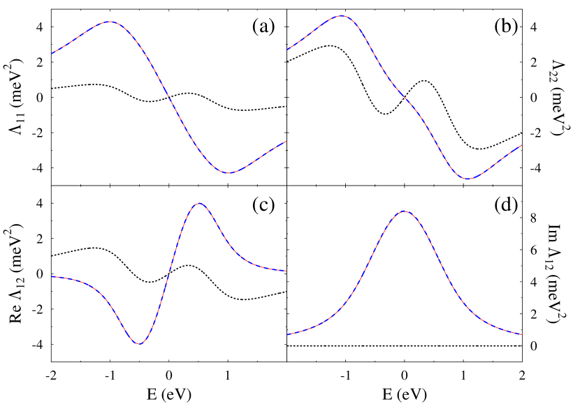
Figure 2: Friction tensor $\Lambda(E)$ for the noninteracting junction model (Fig. 1). Results of the NEGF calculation Lü et al. (2012) (solid line, red) are compared with the Hubbard NEGF (dashed line, blue) and non-equilibrium generalization of the Head-Gordon and Tully electronic friction Head-Gordon and Tully (1995) (dotted line, black). See text for parameters.

Figure 2 shows elements of $\Lambda_{\alpha\beta}(E)$ as obtained from the NEGF and Hubbard NEGF simulations. It is interesting to note that although system-bath coupling $\Gamma$ is not small and while the Hubbard NEGF is perturbative in system-bath coupling strength expansion, Hubbard simulations follow exact (for the model) NEGF results very closely. Similar accuracy in a wide range of parameters was noted in our recent publication Miwa et al., 2017. We attributed the effect to similarity of diagrammatic techniques for the two Green functions.

We also compare the results with a generalized version of the Head-Gordon and Tully friction tensor Head-Gordon and Tully (1995). In our model this generalization is given by $D^{r}_{ab,ba}$ and $D^{r}_{ba,ba}$ contributions in Eq. (28). Here $a$ and $b$ are molecular many-body states with one electron being in one of eigenstates of the Hamiltonian $H^{0}$. As expected, at non-negligible system-bath coupling this form of the tensor fails to reproduce correct behavior (see Fig. 2). Naturally, with decrease in the system-bath coupling $\Gamma$ the Head-Gordon and Tully result becomes more accurate (especially at the energies corresponding to transitions between molecular eigenstates; see Fig. S1 in SM Chen et al. (2018)).

Figure 3 demonstrates relative importance of the Berry phase force. Also here, the Hubbard NEGF calculations closely follow exact (for the model) NEGF results. As was first indicated in Ref. Lü et al., 2012, Berry force is pronounced at energies corresponding to transitions between molecular many-body states. Its significance decreases with separation between transition energy and chemical potential.

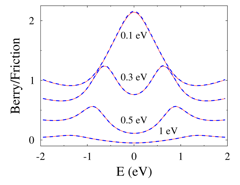
Figure 3: The Berry phase force relative to the average friction. Results of the NEGF calculation Lü et al. (2012) (solid line, red) are compared with the Hubbard NEGF (dashed line, blue). Numbers indicate position of the level $\epsilon_{0}$. Parameters are as in Fig. 2.

Finally, short discussion of non-Condon effects in current-induced forces is given in SM Chen et al. (2018). We postpone detailed study to future publication.

Conclusion. We presented general derivation of current-induced forces for non-adiabatic nuclear dynamics and compared it to previous works. Our derivation goes beyond the usually assumed extremely slow (Ehrenfest) nuclear dynamics. Thus, resulting expressions for the forces are applicable also in intermediate regime (for example, in combination with surface-hopping schemes). The derivation is completely general in a sense that it is applicable in equilibrium and non-equilibrium molecular systems which may be open or closed, with or without intra-molecular interactions (e.g., electron-electron repulsion) taken into account, and for any electron-nuclear coupling. The derivation is based on a standard cumulant expansion, i.e. it is a first principles consideration, which allows for consistent extension of the treatment into higher (than the utilized second) orders. Results of previous works follow from our derivation as particular limiting cases. We established connection with the Zubarev’s method of nonlinear statistical operator. This opens a practical way for considerations beyond strictly adiabatic limit. We also discussed effective ways of evaluating friction tensor in interacting nonequilibrium systems. In particular, we show that recently introduced by us nonequilibrium diagrammatic technique for the Hubbard Green functions Chen et al. (2017) may be a convenient tool for evaluation of the friction tensor. For example, usual expressions for the tensor in interacting systems require consideration of two-particle Green function; the same consideration requires evaluation of only single-particle Hubbard Green function. Main goal of this study is to demonstrate a consistent general derivation. Application of the methodology to actual calculations and elucidation of the role of non-adiabatic driving are goals of future research.