Exotic Gravitational Wave Signatures from Simultaneous Phase Transitions

Abstract

We demonstrate that the relic gravitational wave background from a multi-step phase transition may deviate from the simple sum of the single spectra, for phase transitions with similar nucleation temperatures $T_{N}$. We demonstrate that the temperature range $\Delta T$ between the volume fractions $f(T)=0.1$ and $f(T)=0.9$ occupied by the vacuum bubbles can span $\sim 20$ GeV. This allows for a situation in which phase transitions overlap, such that the later bubbles may nucleate both in high temperature and intermediate temperature phases. Such scenarios may lead to more exotic gravitational wave spectra, which cannot be fitted that of a consecutive PTs. We demonstrate this explicitly in the singlet extension of the Standard Model. Finally, we comment on potential additional effects due to the more exotic dynamics of overlapping phase transitions.

1 Introduction

The detection of gravitational waves (GW) Abbott:2016blz established an important probe of New Physics. Deviations in the waveform of resolvable events could point to interacting dark matter Ellis:2017jgp ; Croon:2017zcu , exotic compact objects Giudice:2016zpa ; Palenzuela:2017kcg ; Croon:2018ftb or the fracturing of condensates Kusenko:2008zm ; Kusenko:2009cv . The observation also implies that the detection of a stochastic GW background will be within reach of current and future detectors. This may be a rare probe of the Cosmic Dark Ages and the first observational window onto cosmic phase transitions (PTs). Such a cosmic phase transition leaves behind a striking relic gravitational wave spectrum that depends on the strength of the transition, the speed of the transition, the bubble wall velocity and the temperature of the transition. The electroweak phase transition in particular is of interest since a strongly first order electroweak phase transition can catalyze electroweak baryogenesis White:2016nbo ; Morrissey:2012db ; Trodden:1998ym ; Dev:2016feu providing an explanation for matter anti-matter asymmetry observed today deVries:2017ncy ; Balazs:2016yvi ; Akula:2017yfr ; Balazs:2013cia ; Balazs:2004ae ; Lee:2004we ; Morrissey:2012db ; Trodden:1998ym . The phenomenology of such PTs have been studied abundantly Balazs:2016tbi ; Jinno:2017ixd ; Matsui:2017ggm ; Huang:2017kzu ; Baldes:2017ygu ; Demidov:2017lzf ; Chala:2018ari ; Hashino:2018zsi ; Kobakhidze:2016mch ; Arunasalam:2017ajm and the GW production has recently been advanced theoretically Hindmarsh:2016lnk and through lattice simulations Hindmarsh:2017gnf ; Cutting:2018tjt .

Recently there has been much interest in multi-step phase transitions Patel:2013zla ; Inoue:2015pza ; Akula:2017yfr ; Vieu:2018zze ; Ramsey-Musolf:2017tgh ; Kang:2017mkl ; Patel:2012pi ; Blinov:2015sna . The electroweak phase transition can occur at a higher scale, if the symmetry breaks through a two step transition Inoue:2015pza . Baryogenesis can occur through exotic high temperature color breaking transitions Ramsey-Musolf:2017tgh and if a singlet acquires a vev before the electroweak phase transition, it can catalyze a strongly first order electroweak phase transition Profumo:2014opa as well as affecting the amount of baryon asymmetry produced in the NMSSM Akula:2017yfr . Here we will consider the GW signal from multi-step phase transitions, and argue that the phenomenology may be altered if the transitions overlap. To show this, here we will compare the different situations,

• Isolated phase transitions; phase transitions which are separated in temperature from other PT. For sequential isolated PTs, the GW signal is expected to be the sum of both spectra.

• Simultaneous phase transitions; the phase transitions overlap and bubbles of both vaccua coexist for some range $\Delta T$. As we will argue here, the GW signal is expected to deviate from the sum of single spectra, as the evolution of the bubbles may be altered.

As an example, we will study a common multi-step PT in a singlet scalar boson extension of the Standard Model. Such new bosons are ubiquitous in extensions to the Standard Model Chang:2017ynj ; Chang:2012ta ; Ng:2015eia ; Ellwanger:2010oug ; Athron:2009bs ; Balazs:2013cia ; Akula:2017yfr ; Ivanov:2017dad ; Fink:2018mcz ; Vieu:2018nfq ; Croon:2015naa ; Aydemir:2015nfa ; Aydemir:2016xtj ; Croon:2015wba . New scalar particles can be a dark matter candidate, the inflaton Croon:2013ana , a portal to the dark sector Chang:2016pya ; Chang:2014lxa ; Cabral-Rosetti:2017mai ; Garg:2017iva ; McKay:2017iur ; Athron:2017kgt ; Burgess:2000yq ; McDonald:1993ex ; Cline:2013gha , as well as a catalyzing a strongly first order electroweak phase transition Profumo:2014opa ; Profumo:2007wc ; White:2016nbo ; Kozaczuk:2014kva and improving the stability of the vacuum EliasMiro:2012ay ; Gonderinger:2009jp ; Gonderinger:2012rd ; Khan:2014kba ; Balazs:2016tbi . GW detection provides a complimentary probe to this model to current and future colliders Chang:2018pjp ; Contino:2016spe .

This paper is organized as follows. In the next section, we will give a brief review of the parameters that influence the evolution of the nucleation rate and growth of vacuum bubbles. In section 3, we will describe the different nucleation cases, and show the effects in a toy model example. In section 4, we will provide a more realistic application of the coexisting PT, in a singlet extension of the Standard Model. We will finish with a summary and an outlook to the experimental prospects of these effects.

2 Thermal parameters for a cosmic phase transition

2.1 Review of important parameters

For a system with multiple scalar fields evolving with temperature during a cosmic phase transition, many thermal properties are controlled by the euclidean action

$$S_{\rm E}=4\pi\int r^{2}dr\left[\sum_{i}\frac{1}{2}\left(\frac{\partial\phi_{i}}{\partial r}\right)^{2}+V(\phi_{i},T)\right]$$ (1)

where we have assumed spherical symmetry for the system. The extremum of the euclidean action that describes the formation of a bubble of a new phase forming in a vacuum of high temperature phase is called the bounce Coleman:1977py ; Callan:1977pt ; Linde:1980tt . The bounce is a solution to the classical equations of motion

$$\frac{\partial^{2}\phi_{i}}{\partial r^{2}}+\frac{2}{r}\frac{\partial\phi_{i}}{\partial r}=\frac{\partial V}{\partial\phi_{i}}$$ (2)

with boundary conditions $\phi_{i}(0)\sim\phi_{i}(v_{i})$, $\phi_{i}^{\prime}=0$ and $\phi_{i}(\infty)=(v_{i}^{0})$ where $v_{i}$ and $v_{i}^{0}$ are the true and false vacua respectively. The transition temperature $T_{N}$ is defined as the temperature when at least one critical bubble forms within a Hubble volume and is approximately given by

$$\frac{S_{E}}{T_{N}}\sim 177-4\ln\frac{T_{N}}{\rm GeV}-2\ln g_{*}$$ (3)

with some uncertainty in the initial numeric factor on the right hand side. The characteristic rate of bubble nucleation $\beta$ is given by

$$\frac{\beta}{H}=T\frac{\partial}{\partial T}\left(\frac{S_{E}}{T}\right)\ .$$ (4)

A quantity related to the latent heat of the system, $\Upsilon$, is also relevant to the relic gravitational wave background and is defined as

$$\Upsilon=\frac{\rho}{\rho^{*}}$$ (5)

where $\rho^{*}$ is the energy density for a radiation dominated universe, and $\rho$ the difference in energy density in the vacuua on either sides of the bubble wall,

$$\rho^{*} = \frac{g_{*}\pi^{2}T^{4}}{30}$$ (6)

$$\rho = \left.\left[V-\frac{\partial V}{\partial T}T\right]\right|_{v_{i}^{0}}-\left.\left[V-\frac{\partial V}{\partial T}T\right]\right|_{v_{i}}\ .$$ (7)

The wall velocity can also be calculated from the finite temperature effective potential $V(T,\phi^{i})$ White:2016nbo . In the slow and fast wall regimes, the wall velocity can be calculated semi-analytically. However, for the case of Standard Model plus singlet the usual approximations for calculating the wall velocity White:2016nbo can break down, making the calculation of the wall velocity a formidable task Kozaczuk:2015owa . We refer the reader to Kozaczuk:2015owa for an explicit numerical computation. Here we note that a typical wall velocity is $0.2\leq v_{w}\leq 0.6$ for the electroweak transition, but may vary from $v_{w}\sim 0.01$ and $v_{w}\rightarrow 1$ depending on the medium in which the bubble expands. Specifically, the wall velocity is controlled by “friction terms” provided by the particles which change rest mass in the PT. The amount of friction depends on the magnitude of the mass change, and the distribution of such particles in the plasma. In particular, the wall velocity may reach ultra-relavistic values for a PT in a vacuum Kosowsky:1991ua .

The final thing we will need is the growth of the volume fraction as a function of time. First, the transition rate is Linde:1980tt

$$\Gamma=T^{4}\left(\frac{S_{E}}{2\pi T}\right)^{3/2}e^{-S_{E}/T}\ .$$ (8)

From this we can calculate the number of bubbles in a Hubble volume Anderson:1991zb ; Caprini:2011uz

$$N(T)=\int_{T}^{T_{C}}\frac{dT}{T}\frac{\Gamma}{H(T)^{4}}$$ (9)

with the Hubble parameter in equilibrium,

$$H(T)=\left[\frac{8\pi g_{*}T^{4}}{90m_{\rm pl}^{2}}\right]^{1/2}$$ (10)

Then, we can write the new phase volume fraction as

$$f(T) = N(T)\times\frac{4\pi}{3}\frac{\left(R_{c}+v_{w}t\right)^{3}}{H(T)^{-3}}$$ (11)

$$= N(T)\times\frac{4\pi}{3}\left(R_{c}+v_{w}\left[\frac{1}{T^{2}}-\frac{1}{T_{N}^{2}}\right]\sqrt{\frac{45}{16\pi^{3}}}\frac{m_{\rm pl}}{g_{*}}\right)^{3}H(T)^{3}$$ (12)

Note that in the above we have $R_{c}=\delta(T)v_{s}(T)/\Lambda^{2}(T)$ in the notation for the singlet PT (in section 4). We show an example of the evolution of $f(T)$ in Fig. 1. The PT finishes at $T_{f}$, which is defined by

$$f(T_{f})=1$$ (13)

The duration of the PT is then given by $\Delta T=T_{f}-T_{N}$, and can be up to $\mathcal{O}(10\,\text{GeV})$, as is seen from Fig.1. As is obvious, simultaneous PT are more likely for relatively large $\Delta T$.

Figure 1: Benchmark example for the volume fraction (11) as a function of temperature. For this benchmark, $T_{c}=196\text{ GeV}$ and $v(T_{c})=225\text{ GeV}$.

Finally, we will comment on the duration of the PT with respect to reheating and the Hubble parameter. For a radiation dominated Universe, the temperature and time are related by

$$T^{2}t=\sqrt{\frac{45}{16\pi^{3}}}\frac{M_{p}}{g_{*}}\ .$$ (14)

In a more general scenario the relationship between temperature and time is more involved, as the production of bubbles releases latent heat which reheats the vanilla vacuum. The amount of reheating decreases with $x=g_{l}/g_{*}$ where $g_{l}$ is the number of degrees of freedom that don’t acquire a mass through the phase transition Megevand:2007sv . However, in the case of the singlet phase transition $g_{l}\sim g_{*}$, and the reheating is therefore small. Furthermore, since the bubble wall velocities are assumed to be relatively fast for our analysis, we do not expect the latent heat to diffuse throughout the vanilla vacuum. Therefore we will assume that the relevant temperature range in the vanilla vacuum will not be affected by reheating, for the majority of the volume. We note that for $\Delta T=10$ GeV, the duration of the PT is $\sim 10^{-10}$ s. Since this is much shorter than the Hubble scale at the time of the PT, $H_{*}^{-1}$, we ignore Hubble expansion in the following. For an analysis where this assumption is relaxed see Kobakhidze:2017mru

2.2 Coexisting bubbles: $T_{N}^{(1)}>T_{N}^{(2)}>T_{f}^{(1)}$

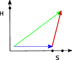
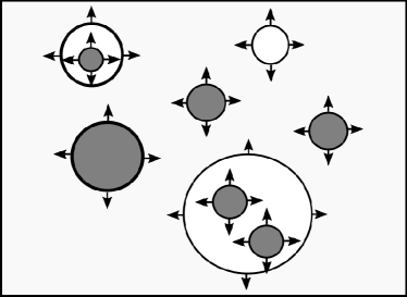
Figure 2: Left: the possible phase transitions for the case where the Standard Model is extended by a singlet. If the phase transitions are separated then only either bubbles for the blue and red transitions form. If the phase transitions are overlapping the green can form too. Right: Example of the nucleation of different bubble species when an overlapping two step phase transition occurs. The background is the vanilla vacuum and different coloured bubbles represent the vacua A and B, corresponding to minima which are deeper than the vanilla vacuum.

Now we will consider the case where the Standard Model is extended by a singlet scalar field. The vacuum transitions that can occur in a two step transition are shown in the left panel of Fig. 2. In the case where $T_{N}^{(1)}>T_{N}^{(2)}>T_{f}^{(1)}$, bubbles for the first transition may form in the vanilla vacuum, and bubbles of the true vacuum may form in both the singlet and vanilla phases as shown in the right panel of Fig. 2. This scenario can occur when there is a zero temperature barrier between the true and false vacuum in the singlet sector. In this case, $S_{E}/T$ decreases until there is a minimum, followed by a period in which then $S_{E}/T$ increases as the universe cools. Examples of this are shown in Fig. 6. In these cases, where $S_{E}/T$ only drops slightly below the critical value (defining the nucleation temperature), the difference between $T_{N}$ and $T_{f}$ can be tens of GeV, as shown for an explicit example in Fig. 1. Here, the $\Delta T$ taken for the volume fraction of the new phase to grow from $0.1$ to $1$ is $\sim 20$ GeV.

Eventually the temperature is low enough so that the second species of bubble forms. If the second bubble forms within the first bubble, it will have a different transition temperature, latent heat, transition speed and wall velocity compared to the case where it forms in the vanilla vacuum. In the following, we will denote the latter as $\{\Upsilon_{2},\beta_{2}/H,T_{N}^{(2)},v_{w}^{(2)}\}$ and the former as $\{\Upsilon_{3},\beta_{3}/H,T_{N}^{(3)},v_{w}^{(3)}\}$. Particularly, we expect the friction within another bubble to be typically less than in the vanilla vacuum, as the fractional change in masses is smaller. There is also a smaller $\Upsilon$ as there is typically a smaller difference between the potentials of the bubbles than between the second bubble and the vanilla vacuum. It is more involved to see the difference in the transition rates, as these depend on the size of the barrier between the transitions. For our benchmarks we find that all transitions are strongly first order. Lastly, we also expect a change in transition temperature between scenarios 2) and 3).

Finally, we want to comment on the collision of bubbles of different vacuum. Such bubbles will not merge, but the bubble corresponding to the deeper vacuum can consume the other. The process can be understood as follows. Near the two bubble walls the field must continuously evolve, in both field space and space-time. It will then be energetically favourable for the bubble wall of the deeper vacuum to advance forward. However, even without collision, the consumption of a bubble may lead a forth contribution to the relic gravitational waves, since the plasma shells of the two different species of bubbles could interact, potentially creating another sound wave contribution. Understanding the potential production of gravitational waves from such a process would require a precise numerical simulation, so we will leave this for future work.

3 Gravitational waves from multi-step phase transitions

3.1 Gravitational wave spectrum

First order cosmological phase transitions proceed via bubble nucleation. Upon collisions of such bubbles, the latent heat will be converted to bulk flow of the plasma, as well as to kinetic energy of the scalar fields. The contributions to the GW spectrum of the latter are well captured by the envelope approximation Huber:2008hg , but the contributions from the plasma flow are much harder to capture in a model. Moreover, recent studies indicate Hindmarsh:2017gnf that the plasma flow contributions dominate over the scalar field contributions, since the plasma flow continues to source GWs long after the collisions of the bubbles.

Progress in this area has been largely dominated by large-scale hydrodynamic simulations. Nevertheless, well-motivated simplified models have been developed recently, such as the recent bulk flow model Jinno:2017fby and sound shell model Hindmarsh:2016lnk . Such models may describe the physics in regimes in where simulations have limitations Konstandin:2017sat .

The gravitational wave spectrum produced by a cosmic phase transition can be written in terms of a sum of three contributions - a collision term describing the collision of bubbles, a sound wave term describing the interaction of plasma shells after a collision and finally a turbulence term. Here, we will adopt a parametrization from Weir:2017wfa to capture the essential features of the spectrum as follows:

$$\Omega_{\rm GW}=\Omega_{\rm env}+\Omega_{\rm sw}+\Omega_{\rm turb}$$ (15)

However, our analysis can straightforwardly adapted when future models become available. Following Weir:2017wfa , the collision term is given by

$$h^{2}\Omega_{\rm col}=1.67\times 19^{-5}\left(\frac{0.48v_{w}^{3}}{1+5.3v_{w}^{2}+5v_{w}^{4}}\right)\left(\frac{\beta}{H}\right)^{-2}\kappa_{\rm col}^{2}\left(\frac{\Upsilon}{1+\Upsilon}\right)^{2}\left(\frac{100}{g_{*}}\right)^{1/3}S_{\rm col}(f)$$ (16)

The efficiency parameter $\kappa_{\phi}$ is typically vanishingly small, making this contribution sub-dominant. For $v_{w}$ close to unity one has for the frequency spectrum,

$$S_{\rm col}=\left[c_{l}\left(\frac{f}{f_{\rm col}}\right)^{-3}+(1-c_{l}-c_{h})\left(\frac{f}{f_{\rm col}}\right)^{-1}+c_{h}\left(\frac{f}{f_{\rm col}}\right)^{-1}\right]\ .$$ (17)

Fitting yields $c_{l}=0.064$ and $c_{h}=0.48$ Weir:2017wfa , as well as

$$f_{\rm col}=1.65\times 10^{-7}{\rm Hz}\left(\frac{0.35}{1+0.069v_{w}+0.69v_{w}^{4}}\right)\left(\frac{\beta}{H}\right)\left(\frac{T_{N}}{\rm GeV}\right)\left(\frac{g_{*}}{100}\right)^{1/6}\ .$$ (18)

The sound wave contribution is typically larger. Its power spectrum is

$$h^{2}\Omega_{\rm sw}=8.5\times 10^{-6}\left(\frac{100}{g_{*}}\right)^{-1/3}\Gamma^{2}\bar{U}_{f}^{4}\left(\frac{\beta}{H}\right)^{-1}v_{w}S_{\rm col}(f)$$ (19)

where $\Gamma\sim 4/3$ is the adiabatic index, and $\bar{U}_{f}^{2}\sim(3/4)\kappa_{f}\alpha_{T}$ is the rms fluid velocity. The efficiency parameter is in this case given by

$$\kappa_{f}\sim\frac{\Upsilon}{0.73+0.083\sqrt{\Upsilon}+\Upsilon}$$ (20)

and the spectral shape is given by

$$S_{\rm sw}=\left(\frac{f}{f_{\rm sw}}\right)^{3}\left(\frac{7}{4+3\left(\frac{f}{f_{\rm sw}}\right)^{2}}\right)^{7/2}$$ (21)

with

$$f_{\rm sw}=8.9\times 10^{-7}{\rm Hz}\frac{1}{v_{w}}\left(\frac{\beta}{H}\right)\left(\frac{T_{N}}{{\rm Gev}}\right)\left(\frac{g_{*}}{100}\right)^{1/6}\ .$$ (22)

Finally, for the turbulence contribution we have

$$h^{2}\Omega_{\rm turb}(f)=3.35\times 10^{-4}\left(\frac{\beta}{H}\right)^{-1}\kappa_{\rm turb}^{3/2}\left(\frac{\Upsilon}{1+\Upsilon}\right)^{3/2}\left(\frac{100}{g_{*}}\right)^{1/3}v_{w}S_{\rm turb}(f)$$ (23)

where we may take $\kappa_{\rm turb}\sim 10^{-4}$, making this contribution also sub-dominant. The spectrum is

$$S_{\rm turb}=\frac{(f/f_{\rm turb})^{3}}{\left[1+(f/f_{\rm turb})\right]^{11/3}(1+8\pi f/h*)}$$ (24)

with

$$h_{*} = 1.65\times 10^{-7}{\rm Hz}\left(\frac{T_{N}}{{\rm GeV}}\right)\left(\frac{g_{*}}{100}\right)^{1/6}$$ (25)

$$f_{\rm turb} = 27\times 10^{-7}{\rm Hz}\frac{1}{v_{w}}\left(\frac{\beta}{H}\right)\left(\frac{T_{N}}{\rm GeV}\right)\left(\frac{g_{*}}{100}\right)^{1/6}$$ (26)

The above contributions were estimated in the case of a single phase transition, which completes quickly, so the thermal parameters at the nucleation temperature are to model the gravitational wave spectrum. In our case the thermal parameters vary considerably during the phase transition as can be seen by Fig. 6. This is due to the first phase transition completing over $\Delta T\sim 20$ GeV. As such we expect there to be a large numerical uncertainty in applying these fits to our scenario. This source of uncertainty we leave to future simulations. We will, however estimate the effects of overlapping transitions in the next subsection, based on the spectra of single PTs above.

3.2 Overlapping phase transitions

In the case of overlapping phase transitions there are different thermal parameters, corresponding to different situations which we cover in this subsection. We will make the simplifying assumption that the thermal parameters are determined by the nucleation scenario of the bubbles. In reality, the thermal parameters may evolve, which may be modeled in a future numerical analysis. Throughout this paper we model the peak amplitude, frequency and spectrum produced by these situations as a weighted sum of the different nucleation situations as follows,

$$\Omega_{GW}=\sum_{i}w_{i}\,\Omega_{GW}^{(i)}\left(\Omega_{0}^{(i)},f^{(i)},\Upsilon_{i},v_{w}^{(i)},\frac{\beta^{(i)}}{H},T_{N}^{(i)}\right)\ .$$ (27)

Here the index $i$ characterizes the nucleation scenario. For example, for the simultaneous PTs to vacua A and B, one may have (conf. Fig. 2),

1. Vacuum A $(v_{A},0)$ in the vanilla vacuum $(i=1)$;

2. Vacuum B $(v_{A},v_{B})$ in the vanilla vacuum $(i=2)$;

3. Vacuum B $(v_{A},v_{B})$ in vacuum A $(i=3)$.

Each of these situations will in principle be described by different parameters $(v_{w}^{(i)},\Upsilon_{i},\beta^{(i)})$. Then, $w_{i}(t)$ characterizes the relative importance of the nucleation scenarios, which we will estimate in the following way. First, we note that if there are different nucleation scenarios of the same vacuum, the definition of $T_{f}$ (Eq. (13)) should change, to reflect that the PT finishes when the vacuum has filled all of space-time,

$$\mathop{{\sum}}\limits_{j\in\text{vacuum$(i)$}}f_{j}\left(\tilde{T}_{f}^{(i)}\right)=1\,\,\,\,\,\,\,\,\,\,\,\,\text{PT completes}$$ (28)

where $f_{i}(T)$ is evaluated at $v_{w}^{(i)},\Upsilon_{i},\beta^{(i)}$, corresponding to the nucleation scenario. Explicitly, in the above example, this means that transitions 2. and 3. both finish at $\tilde{T}^{(2)}_{f}=\tilde{T}^{(3)}_{f}$, when

$$f_{2}\left(\tilde{T}^{(2)}_{f}\right)+f_{3}\left(\tilde{T}^{(2)}_{f}\right)=1.$$

For a schematic representations, see Fig. 3.

It is important to note that for simultaneous transitions, the earlier PT may not reach completion, as the consecutive PT takes over before $f_{i}(T)=1$ is reached. In the above example, this applies to the first transition. In such cases Eq. (13) also breaks down. Instead, we may estimate the final temperature $\tilde{T}_{f}$ by

$$\mathop{{\sum}}\limits_{j\in\text{vacuum$(i)$}}f_{j}\left(\tilde{T}_{f}^{(i)}\right)+\mathop{{\sum}}\limits_{k\not\in\text{vacuum$(i)$}}f_{k}\left(\tilde{T}_{f}^{(i)}\right)=1\,\,\,\,\,\,\,\,\,\,\,\,\text{PT does not complete}$$ (29)

such that the earlier PT is cut-off when the later PT has caught up.

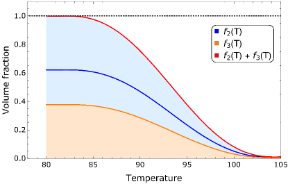
Figure 3: Example of relative weight factors for two nucleation scenarios of the same vacuum.

Thus, summarizing (28) and (29), the final temperatures of simultaneous PTs can be estimated by,

$$\mathop{{\sum}}\limits_{j\in\text{vacuum$(i)$}}f_{j}\left(\tilde{T}_{f}^{(i)}\right)=\begin{cases}1&\text{PT completes}\\ 1-\mathop{{\sum}}\limits_{k\not\in\text{vacuum$(i)$}}f_{k}\left(\tilde{T}_{f}^{(i)}\right)&\text{PT does not complete}\end{cases}$$ (30)

Then, the weight factor can be approximated by,

$$w_{i}=\frac{\mathop{{\int}}^{\tilde{T}^{(i)}_{f}}_{T^{(i)}_{N}}f_{i}(T)dT}{\mathop{{\int}}_{\tilde{T}^{(i)}_{N}}^{\tilde{T}^{(i)}_{f}}\left[\mathop{{\sum}}\limits_{j\in\text{vacuum$(i)$}}f_{j}(T)\right]dT}\,\,\,\,\,\,\,\,\,\text{PT completes}$$ (31)

for PT which complete. It is seen that for consecutive phase transitions, which are separated in time, there is only a single nucleation scenario for each vacuum, such that (31) gives $w_{i}=1,\,\,\forall i$ as expected. The spectrum (27) is in this case a simple sum of the individual spectra. In the case that there are different nucleation scenarios of a vacuum, the $w_{i}$ sum to one. In the above example, we would have $w_{2}+w_{3}=1$. It is seen that any deviations in the spectrum will feature most strongly for $w_{i}\approx w_{j},\,\,j\in\text{vacuum}(i)$.

However, if a PT does not complete, because the following PT takes over, the GW spectrum resulting from this PT will only be a fraction of the spectrum which would have resulted, if the PT had been allowed to finish. Therefore, the $w_{i}$ corresponding to such a vacuum can not sum to one. Here we will estimate it by,

$$w_{i}=\frac{\mathop{{\int}}^{\tilde{T}^{(i)}_{f}}_{T^{(i)}_{N}}f_{i}(T)dT}{\mathop{{\int}}_{T^{(i)}_{N}}^{T^{(i)}_{f}}f_{i}(T)dT}\,\,\,\,\,\,\,\,\,\text{PT does not complete}$$ (32)

where $T_{f}$ corresponds to the end of the vanilla transitions (13) and $\tilde{T}_{f}$ Eq. (30) This insight is an important result of this analysis. It implies that the GW spectrum from simultaneous PT can not be calculated as the sum of consecutive PT.

We note here that we have not taken into account that bubbles of the same vacuum, from different nucleation scenarios, may collide, such that $f^{(i)}(T)$ may overlap. Also, (29) gives an upper bound of the final temperature of a PT which does not complete. As a consequence, the above Eq. (30) may overestimate the final temperature $T_{f}$. Eq. (31) may therefore be considered a conservative estimate of the effect of the simultaneous PT.

3.3 Effects in a toy model

Here we will demonstrate the effects described in the previous section in a toy model. Our toy model will be a hypothetical scenario with two singlet PTs, and is described by the example of the previous sections, and Fig. 2.

The first and most prominent effect of overlapping transitions, is that the first transition may not complete. Therefore, the weight parameter $w_{1}<1$, and the overall spectrum is expected to be weaker. This effect may also cause the double peak of the spectrum to disappear, as shown in the lower left panel of Fig. 4. However, as is shown in the lower right panel of Fig. 4, this spectrum can still not be mimicked by the spectrum from a single PT.

Whether the spectrum has a double peak or a “shoulder”, depends primarily on the difference in nucleation temperature $T_{N}$ between the different scenarios. It is expected that $T_{N}^{(2)}>T_{N}^{(3)}$, i.e., the nucleation temperature inside a bubble of vacuum A is larger than in the vanilla vacuum. Therefore, the double peak is expected to appear for $T_{N}^{(3)}\ll T_{N}^{(1)}$ and $w_{3}\rightarrow 1$, which coincides with the limit of consecutive PT. This is shown in the lower panels of Fig. 4.

One may wonder whether whether the spectrum can be fitted to two consecutive PT. This depends on the relative importance of the weight factors $w_{2}$ and $w_{3}$. For $w_{2}\sim w_{3}$, it is generically not possible to mimic the effect of simultaneous PTs by two consecutive PT, as demonstrated in Fig.5. We note here that the figure shows an idealized situation with an exaggerated difference in nucleation temperatures, to visualize the effect. We will turn to a more realistic model in the following section.

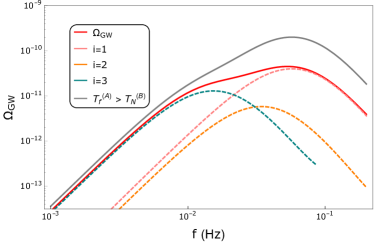
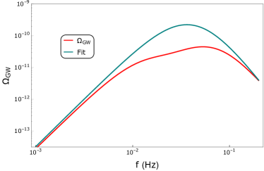
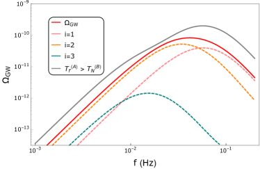
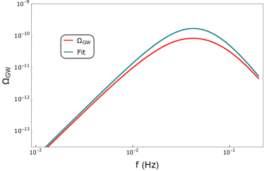
Figure 4: Left panels: the spectrum due to two simultaneous PTs, given by the red line, leads to a different spectrum than consecutive transitions. This can be seen by comparison with the gray line, which is predicted by the same thermal parameters, and $w_{1}=w_{3}=1$, $w_{2}=0$. In the upper example we chose $w_{2}=0.1=1-w_{3}$. In the lower example we chose $w_{2}=0.9=1-w_{3}$. In both examples, $w_{1}=0.2$. Right panels: the spectrum from simultaneous PTs can not be fitted to the spectrum than from a single PT. Shown are fits to $\Omega_{GW}$ in Eq. (15) with $\Upsilon=0.22$, $v_{w}=0.65$, $\beta/H=124$, $T_{N}=134$ GeV (upper panel), and $\Upsilon=0.21$, $v_{w}=0.65$, $\beta/H=142$, $T_{N}=136$ GeV (lower panel).

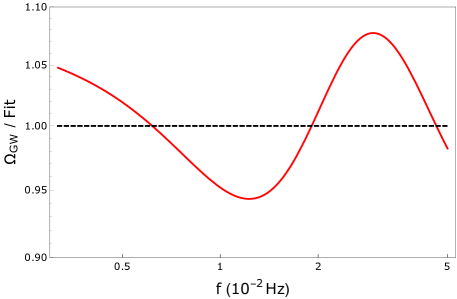
Figure 5: For $w_{2}=w_{3}=0.5$, the spectrum from simultaneous PTs can not be fitted to the spectrum of two single PTs. The comparison is to a fit of $\Omega_{GW}=\Omega_{GW}^{(A)}+\Omega_{GW}^{(B)}$ with the parameters $\Upsilon=0.094$, $v_{w}=0.65$, $\beta/H=77.3$, $T_{N}=115$ GeV (transition A), and $\Upsilon=0.16$, $v_{w}=0.65$, $\beta/H=179$, $T_{N}=133$ GeV (transition B). The frequency band fitted and shown has been chosen such that $\Omega_{GW}>10^{-12}$.

4 Standard Model plus singlet example

The Singlet extension to the Standard Model is not the ideal scenario to demonstrate the effect of an overlapping phase transition visible at LISA as the nucleation temperature tends to be a little low rendering the signal at the edge of what LISA can detect. Nonetheless it is useful as an example to demonstrate how this effect can occur in the simplest extension to the Standard Model as well as a scenario that is desirable for electroweak baryogenesis Profumo:2014opa . The effective potential can be broken up as follows

$${\cal V}=V_{\rm SM}+V_{\rm portal}+V_{\rm singlet}$$ (33)

where

$$V_{\rm SM} = \mu^{2}H^{2}+\frac{\lambda}{4}H^{4}$$ (34)

$$V_{\rm portal} = \frac{\kappa_{1}}{2}SH^{2}+\frac{\kappa_{2}}{2}S^{2}H^{2}$$ (35)

$$V_{\rm Singlet} = M^{2}S^{2}+\kappa S^{3}+\lambda_{s}S^{4}\ .$$ (36)

In our particular choice of the Lagrangian there are terms that explicitly break any $Z_{2}$ symmetry which avoids the problem of cosmologically catastrophic domain walls (see Mazumdar:2015dwd for a discussion of various solutions to domain wall problems). The two parameters in the Standard Model potential are fixed by the mass of the Higgs and the W boson (which determines the Standard Model VEV) respectively. In the Standard Model one has at the electroweak scale $O(100)$ GeV, $\mu^{2}\sim 3848$ GeV and $\lambda\sim 0.25$. When the singlet acquires a vacuum expectation value, one needs to correct the values of the Higgs sector parameters such that the mass of the Higgs and W boson coincide with their measured values. For the mass range we are interested in $|\sin\theta|\lesssim 0.2$ Chalons:2016jeu ; Ilnicka:2018def although future colliders are expected to improved this bound Chang:2018pjp ; Kotwal:2016tex . In principle, a lower bound on the mixing angle can be found from BBN, since long lived particles may interfere with light element production Fradette:2017sdd . However, for the parameter space we consider here, the portal couplings have no effect on BBN, but are instead probed by colliders. The range of portal couplings needed to catalyse a strongly first order electroweak phase transition typically requires $|\kappa 1|$ to be negative with the approximate range $-500\lesssim\kappa 1\lesssim-100$ and $\kappa_{2}\sim O(1)$. Further more ref. Profumo:2014opa found that the portal couplings are anti-correlated for phenomelogically viable parameter sets that result in a strongly first order electroweak phase transition. This anti-correlation suppresses the off diagonal elements in the mass matrix causing the mixing angle to be small.

Finally for the singlet part of the potential it is convenient to reparametrize the potential such that the inputs of the potential are the scale of the potential, the local minimum and a parameter which controls the size of the barrier between the origin and the singlet minimum. Such a parametrization was given in ref. Akula:2016gpl

$$V_{\rm Singlet}=\Lambda^{4}\left[\frac{3-4\alpha}{2}\left(\frac{s^{2}}{v_{s}^{2}}\right)-\left(\frac{s^{3}}{v_{s}^{3}}\right)+\alpha\left(\frac{s^{4}}{v_{s}^{4}}\right)\right]\ .$$ (37)

Where scale of the potential is given by $\Lambda$, the singlet vev is denoted $v_{s}$ and $\alpha\in[0.5,0.75]$ parametrizes the size and location of the tree level barrier between the true ($v_{s}$) and false vacuum ($0$). Here $\alpha=0.5$ corresponds to degenerate minima and $\alpha=0.75$ corresponds to the case where there is no barrier. The critical temperature and the mass of the singlet are both approximately the scale of the potential. That is $\Lambda\sim M_{s}\sim T_{N}$ up to an order one factor. Since we want the transition to overlap with the electroweak phase transition we require $\Lambda\sim m_{H}$.

The nucleation temperature, $T_{N}$, is lower than the critical temperature by an amount

$$T_{N}=(1-\epsilon)T_{C}$$ (38)

where a large epsilon corresponds to the case where there is a lot of supercooling. The amount of supercooling is largest for smaller $\alpha$ and larger $v_{S}$. To ensure the two phase transitions are close together we require $v_{S}\sim v_{\rm SM}$. Finally the strength of the phase transition is parametrized by the order parameter $\phi_{C}/T_{C}$ and is controlled by $\alpha$ and $v_{S}$ where a larger $v_{S}$ and a smaller $\alpha$ correspond to a stronger phase transition.

	$\Upsilon_{i}$	$v_{w}$	$T_{N}^{i}$	$\beta/H$
$i=1$	$0.22$	$0.69$	$120$	$29.0$
$i=2$	$0.20$		$72.0$	$13.8$
$i=3$	$0.076$		$61.3$	$161.5$
$i=1$	$0.14$	$0.84$	$116$	$33.2$
$i=2$	$0.10$		$70.0$	$40.8$
$i=3$	$0.075$		$65.0$	$128$
$i=1$	$0.29$	$0.58$	$106$	$42.7$
$i=2$	$0.10$		$70.0$	$4.10$
$i=3$	$0.077$		$57.0$	$183$

Table 1: Inputs to relic gravitational wave spectrums for all four SM + singlet benchmarks

$\kappa_{1}$	$\kappa_{2}$	$\Lambda$	$\alpha$	$v_{S}$	$\sin\theta$
$-295$	$0.850$	$120$	$0.61$	$299$	$0.18$
$-300$	$0.900$	$109$	$0.62$	$300$	$0.11$
$-390$	$1.35$	$120$	$0.59$	$249$	$0.074$

Table 2: Lagrangian parameters for the four benchmarks for SM+S as well as the mixing angle $\sin\theta$. Higgs sector parameters are determined by fixing the mass of the Higgs and W boson. All dimensionful parameters are given in GeV.

4.1 High temperature corrections

For simplicity we assume that the mixing is sufficiently small (for our benchmarks $\sin\theta<0.1$) and that we can use the high temperature expansion in the Landau gauge such that the temperature corrections to the effective potential can be approximated in the high temperature expansion and the limit of no mixing as

$$V_{\rm SM} \to (\mu^{2}+c_{h}T^{2})h^{2}-E_{h}Th^{3}+\frac{\lambda}{4}H^{4}$$ (39)

$$V_{\rm portal} \to \kappa_{1}SH^{2}+\frac{\kappa_{2}}{2}S^{2}H^{2}$$ (40)

$$V_{\rm Singlet} \to \Lambda^{4}\left[\left(\frac{3-4\alpha}{2}+c_{s}\frac{T^{2}v_{s}^{2}}{\Lambda^{4}}\right)\left(\frac{s^{2}}{v_{s}^{2}}\right)-\left(1+\frac{E_{s}Tv_{s}^{3}}{\Lambda^{4}}\right)\left(\frac{s^{3}}{v_{s}^{3}}\right)+\alpha\left(\frac{s^{4}}{v_{s}^{4}}\right)\right]\ .$$ (41)

In he above we have replaced the quantum fields with the classical fields and defined

$$c_{h} = \frac{1}{32}\left(g_{1}^{2}+3g_{2}^{2}+4y_{t}^{2}+4\lambda\right)$$ (42)

$$E_{h} = \frac{3}{96\pi}\left(2g_{2}^{3}+(g_{1}^{2}+g_{2}^{2})^{3/2}\right)$$ (43)

$$c_{s} = \frac{\alpha}{2}\frac{\Lambda^{4}}{v^{4}_{s}}$$ (44)

$$E_{s} = \frac{2\sqrt{3}}{\pi}\frac{\Lambda^{6}}{v_{s}^{6}}\alpha^{3/2}\ .$$ (45)

In this case the system can be solved semi-analytically, as we demonstrate in the next subsection. Since this work is a proof of principle we leave precise calculations of these phase transitions to future work and we expect our benchmark to approximate the parameters which describe our scenario.

4.2 Semi-analytic treatment of transitions

There are three possible transitions that we are interested in for the case where the singlet has the higher nucleation temperature. They are

$$(0,0) \to (0,v_{s})$$

$$(0,0) \to (v_{h},v_{s}^{\prime})$$

$$(0,v_{s}) \to (v_{h},v_{s}^{\prime})\ .$$ (46)

The first transition is straightforward to deal with analytically. The change in the scale of the potential, $\Lambda$, the minima $v_{s}$ and the parameter $\alpha$ can be determined by simultaneously solving

$$\frac{\Lambda^{4}}{v_{s}^{2}}\left(\frac{3-4\alpha}{2}+\frac{c_{s}T^{2}v_{s}^{2}}{\Lambda^{4}}\right) = \frac{\Lambda^{4}(T)}{v_{s}^{2}(T)}\left(\frac{3-4\alpha(T)}{2}\right)$$ (47)

$$\frac{\Lambda^{4}}{v_{s}^{3}}\left(1+\frac{E_{s}Tv_{s}^{3}}{\Lambda^{4}}\right) = \frac{\Lambda^{4}(T)}{v_{s}^{3}(T)}$$ (48)

$$\frac{\alpha\Lambda^{4}}{v_{s}^{4}} = \frac{\alpha(T)\Lambda^{4}(T)}{v_{s}^{4}(T)}$$ (49)

where the right hand side contain the temperature dependent versions of the parameters on the left hand side. Note the critical temperature is defined as $\alpha(T_{C})=0.5$. Under these definitions the singlet potential becomes

$$V_{\rm Singlet}(T)=\Lambda(T)^{4}\left[\frac{3-4\alpha(T)}{2}\left(\frac{s^{2}}{v_{s}^{2}(T)}\right)-\left(\frac{s^{3}}{v_{s}^{3}(T)}\right)+\alpha(T)\left(\frac{s^{4}}{v_{s}^{4}(T)}\right)\right]\ .$$ (50)

To a reasonable approximation one can calculate the bounce as straightline transition in field space from the true to the false vacuum. In this case the bounce profile can be calculated to within a fraction of a percent to be

$$s(r,T) = \frac{s_{0}[\alpha(T)]}{2}\left\{1-\tanh\left[\frac{r\Lambda^{2}(T)/v_{s}(T)-\delta[\alpha(T)]}{L_{w}[\alpha(T)]}\right]\right\}$$ (51)

$$- \frac{1}{2}\left|\frac{s_{0}[\alpha(T)]}{L_{w}[\alpha(T)]}{\rm Sech}^{2}\left\{\frac{\delta[\alpha(T)]}{L_{w}[\alpha[T]}\right\}\right|e^{-r\Lambda^{2}(T)/v_{s}(T)}$$

note that $L_{w}$ and $\delta$ are dimensionless in the above equation. Curve fitting for the above gives

$$s_{0}[\alpha(T)] = a\left(1-{\rm Tanh}\left[\frac{\alpha(T)-b}{c}\right]\right)+d$$ (52)

$$L_{w}[\alpha(T)] = a+b\frac{|\alpha(T)-0.5|^{c}}{|\alpha(T)-0.75|^{d}}$$ (53)

$$\delta[\alpha(T)] = \sum_{i}\frac{a_{i}}{|\alpha(T)-b_{i}|^{c_{i}}}$$ (54)

The effective action is then given by

$$\frac{S_{E}}{T}=\frac{v_{s}(T)}{T}\frac{v_{s}^{2}(T)}{\Lambda^{2}(T)}10^{g[\alpha(T)]}$$ (55)

$s_{0}$	$\delta$	$L_{w}$	g
$a=1.50$	$a_{i}=\{0.301,2.67,0.711\}$	$a=1.97$	$a=-71.06$
$b=0.718$	$b_{i}=\{0.749,1.53,1.69\}$	$b=6.70$	$b=71.62$
$c=0.0854$	$c_{i}=\{0.558,-77.9,-15.7\}$	$c=2.10$	$c=0.008805$
$d=-0.479$		$d=0.58$	$d=0.009263$

Table 3: List of parameters involved in curve fitting the bounce solution (need to fix sig figs later)

where

$$g[\alpha(T)] = a+b\frac{|\alpha(T)-0.75|^{c}}{|\alpha(T)-0.5|^{d}}$$ (56)

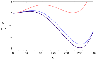
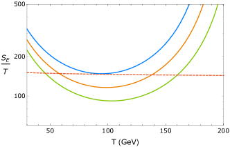
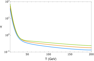
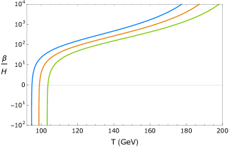
Figure 6: Top left: Evolution of the singlet potential with temperature (top left). The pink curve denotes the potential at the critical temperature, dark blue at the nucleation temperature and light blue at zero temperature. Top right: the evolution of the effective action, bottom left: $\Upsilon$, bottom right: the speed of the phase transition. All with temperature for $v_{s}=260,\alpha=0.6$ and $\Lambda=\{115,125,135\}$ for the green, orange and blue lines respectively.

The nucleation temperature is of course given when equation (3) is satisfied. Let us now turn our attention to the second phase transition where the vanilla vacuum breaks electroweak symmetry and the singlet acquires a vacuum expectation value simultaneously. In this case we can perform the following rotation

$$h = \frac{v_{h}(T)\phi+v_{s}(T)\theta}{\sqrt{v_{s}^{2}(T)+v_{h}^{2}(T)}}$$ (57)

$$s = \frac{-v_{h}(T)\phi+v_{s}(T)\theta}{\sqrt{v_{s}^{2}(T)+v_{h}^{2}(T)}}$$ (58)

where $(v_{h}(T),v_{s}(T))$ is the true vacuum at temperature $T$. Setting $\phi=0$ the potential then looks like

$$\tilde{V} = M_{\theta}(T)\theta^{2}+\kappa_{\theta}\theta^{3}+\lambda_{\theta}\theta^{4}$$ (59)

$$= \Lambda_{\theta}(T)^{4}\left[\frac{3-4\alpha_{\theta}(T)}{2}\left(\frac{\theta^{2}}{v_{\theta}^{2}(T)}\right)-\left(\frac{\theta^{3}}{v_{\theta}^{3}(T)}\right)+\alpha_{\theta}(T)\left(\frac{\theta^{4}}{v_{\theta}^{4}(T)}\right)\right]\ .$$ (60)

We can then use the same semi-analytic techniques to calculate how $S_{E}/T$ evolves with temperature. Finally let us turn our attention to the last transition where a singlet bubble tunnels to a bubble where the singlet has a new minimum and electroweak symmetry is broken simultaneously. Note that this transition may be second order even if the other two are first order. For all of our benchmarks we find it to also be first order. We can treat this transition by making the shift $s^{\prime}=s+v_{s}(T)$ after which we perform similar rotations to before

$$h = \frac{v_{h}(T)\phi^{\prime}+v_{s}^{\prime}(T)\theta^{\prime}}{\sqrt{[v_{s}^{\prime}]^{2}(T)+v_{h}^{2}(T)}}$$ (61)

$$s^{\prime} = \frac{-v_{h}(T)\phi^{\prime}+v_{s}^{\prime}(T)\theta^{\prime}}{\sqrt{[v_{s}^{\prime}]^{2}(T)+v_{h}^{2}(T)}}$$ (62)

where $(v_{h}(T),v_{s}^{\prime}(T))$ is the true vacuum at temperature $T$. Setting $\phi^{\prime}=0$ and dropping primes to avoid clutter we once again have

$$\hat{V} = M_{\theta}(T)\theta^{2}+\kappa_{\theta}\theta^{3}+\lambda_{\theta}\theta^{4}$$ (63)

$$= \Lambda_{\theta}(T)^{4}\left[\frac{3-4\alpha_{\theta}(T)}{2}\left(\frac{\theta^{2}}{v_{\theta}^{2}(T)}\right)-\left(\frac{\theta^{3}}{v_{\theta}^{3}(T)}\right)+\alpha_{\theta}(T)\left(\frac{\theta^{4}}{v_{\theta}^{4}(T)}\right)\right]\ .$$ (64)

4.3 Gravitational wave spectrum

For the Standard Model and singlet scenario, the evolution of the effective potential is shown in Fig. 6 (top left). The evolution of the effective action for the singlet transition is given in the top right panel of Fig. 6. Note that there is a minimum in the effective action. To allow for bubble nucleation, the effective action needs to evolve below the critical value (dotted red line), to allow for bubble nucleation. The PT lasts a long interval $\Delta T$ for a more shallow curve, which only dips a small amount below the critical value. Our benchmarks in Table 1 correspond to such scenarios.

The other panels of Fig. 6 show the evolution of $\Upsilon$ and $\beta/H$ with temperature. Note in particular that $\beta/H$ and $\Upsilon$ change quite quickly during the phase transition. This suggests that there may be some theoretical uncertainty in the gravitational wave spectrum that will be produced, a question which we leave for future numerical simulations. Moreover, $\beta/H$ is fairly small - as you would expect for a phase transition that last a large interval $\Delta T$.

The first benchmark corresponds to the same singlet parameters as the volume fraction of the singlet bubbles we have shown in Fig. 1. In this case, the electroweak phase transition occurs fairly quickly when the singlet bubbles occupy a volume fraction of $\sim 0.5$. The other benchmarks correspond to similar scenarios.

Finally, the gravitational wave spectrum for the third benchmark is given in the left panel of Fig. 7. It seen that the overlapping transition differs from the consecutive case, as before. In the right panel of 7, we demonstrate once more that the spectrum can not be fitted to that of a single PT. It is seen that in particular, it is not possible to fit both the peak and the tails.

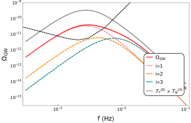
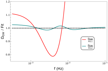
Figure 7: Left panel: the spectrum due to simultaneous singlet and EW PT, given by the red line, leads to a different spectrum than consecutive transitions (gray line). Here we have chosen the second benchmark of Table 1, with $w_{1}=0.1$ and $w_{2}=1-w_{3}=0.15$, and $v^{(2,3)}_{w}=(0.6,0.99)$. The dotted line is the projected sensitivity from LISA AmaroSeoane:2012km . Right panel: comparison of a fit to a single and separated phase transition. It is seen that it is not possible to fit to a single peak spectrum. The fit to a doubly peaked spectrum is better, but still cannot mimic the features in the simultaneous bubble case.

5 Conclusion and Discussion

In this work we have considered the gravitational wave signatures from multi-step phase transitions. We have shown that the phase transition can last an extended interval $\Delta T$, and in such cases bubbles of different vacuum phase can coexist. For such scenarios, the resulting gravitational wave signature is expected to be different from multi-step scenarios which are separated in temperature and can be considered consecutively.

We demonstrated this explicitly by modeling the relative importance of the different nucleation scenarios with weight factors $w_{i}$. We described a toy model involving two scalar fields (weakly coupled to the Standard Model), and a benchmark scenario of a singlet extension to the Standard Model. While the latter is well motivated by a variety of considerations, especially concerning EW baryogenesis, its detection prospects at future gravitational wave experiments such as LISA are modest. The effects described in this paper may be more relevant for multi-step baryogenesis scenarios with multiple singlets, such as described in Ramsey-Musolf:2017tgh ; Inoue:2015pza .

Throughout this work we have mainly considered the sound wave contribution to the gravitational waves (through efficiency parameters $\kappa_{\phi},\kappa_{\text{turb}}\ll 1$), as this contribution is expected to dominate Hindmarsh:2017gnf . In this work it was assumed that the curve fitting to numerical simulations holds in our case where the phase transition proceeds very slowly. Furthermore, we have assumed that the thermal parameters are determined by the nucleation scenario; a more sophisticated analysis will allow these to evolve. We have also not considered the potentially exotic source of gravitational waves, through the interaction between the plasma shells of bubbles of different species. We leave these effects to future studies.

- (1) Virgo, LIGO Scientific collaboration, B. P. Abbott et al., Observation of Gravitational Waves from a Binary Black Hole Merger, Phys. Rev. Lett. 116 (2016) 061102, [1602.03837].
- (2) J. Ellis, A. Hektor, G. Hütsi, K. Kannike, L. Marzola, M. Raidal et al., Search for Dark Matter Effects on Gravitational Signals from Neutron Star Mergers, 1710.05540.
- (3) D. Croon, A. E. Nelson, C. Sun, D. G. E. Walker and Z.-Z. Xianyu, Hidden-Sector Spectroscopy with Gravitational Waves from Binary Neutron Stars, 1711.02096.
- (4) G. F. Giudice, M. McCullough and A. Urbano, Hunting for Dark Particles with Gravitational Waves, JCAP 1610 (2016) 001, [1605.01209].
- (5) C. Palenzuela, P. Pani, M. Bezares, V. Cardoso, L. Lehner and S. Liebling, Gravitational Wave Signatures of Highly Compact Boson Star Binaries, Phys. Rev. D96 (2017) 104058, [1710.09432].
- (6) D. Croon, M. Gleiser, S. Mohapatra and C. Sun, Gravitational Radiation Background from Boson Star Binaries, 1802.08259.
- (7) A. Kusenko and A. Mazumdar, Gravitational waves from fragmentation of a primordial scalar condensate into Q-balls, Phys. Rev. Lett. 101 (2008) 211301, [0807.4554].
- (8) A. Kusenko, A. Mazumdar and T. Multamaki, Gravitational waves from the fragmentation of a supersymmetric condensate, Phys. Rev. D79 (2009) 124034, [0902.2197].
- (9) G. A. White, A Pedagogical Introduction to Electroweak Baryogenesis. IOP Concise Physics. Morgan and Claypool, 2016, 10.1088/978-1-6817-4457-5.
- (10) D. E. Morrissey and M. J. Ramsey-Musolf, Electroweak baryogenesis, New J. Phys. 14 (2012) 125003, [1206.2942].
- (11) M. Trodden, Electroweak baryogenesis, Rev. Mod. Phys. 71 (1999) 1463–1500, [hep-ph/9803479].
- (12) P. S. B. Dev and A. Mazumdar, Probing the Scale of New Physics by Advanced LIGO/VIRGO, Phys. Rev. D93 (2016) 104001, [1602.04203].
- (13) J. de Vries, M. Postma, J. van de Vis and G. White, Electroweak Baryogenesis and the Standard Model Effective Field Theory, JHEP 01 (2018) 089, [1710.04061].
- (14) C. Balazs, G. White and J. Yue, Effective field theory, electric dipole moments and electroweak baryogenesis, JHEP 03 (2017) 030, [1612.01270].
- (15) S. Akula, C. Balázs, L. Dunn and G. White, Electroweak baryogenesis in the -invariant NMSSM, JHEP 11 (2017) 051, [1706.09898].
- (16) C. Balázs, A. Mazumdar, E. Pukartas and G. White, Baryogenesis, dark matter and inflation in the Next-to-Minimal Supersymmetric Standard Model, JHEP 01 (2014) 073, [1309.5091].
- (17) C. Balazs, M. Carena, A. Menon, D. E. Morrissey and C. E. M. Wagner, The Supersymmetric origin of matter, Phys. Rev. D71 (2005) 075002, [hep-ph/0412264].
- (18) C. Lee, V. Cirigliano and M. J. Ramsey-Musolf, Resonant relaxation in electroweak baryogenesis, Phys. Rev. D71 (2005) 075010, [hep-ph/0412354].
- (19) C. Balazs, A. Fowlie, A. Mazumdar and G. White, Gravitational waves at aLIGO and vacuum stability with a scalar singlet extension of the Standard Model, Phys. Rev. D95 (2017) 043505, [1611.01617].
- (20) R. Jinno, S. Lee, H. Seong and M. Takimoto, Gravitational waves from first-order phase transitions: Towards model separation by bubble nucleation rate, JCAP 1711 (2017) 050, [1708.01253].
- (21) T. Matsui, Gravitational waves from the first order electroweak phase transition in the symmetric singlet scalar model, EPJ Web Conf. 168 (2018) 05001, [1709.05900].
- (22) F. P. Huang and C. S. Li, Probing the baryogenesis and dark matter relaxed in phase transition by gravitational waves and colliders, Phys. Rev. D96 (2017) 095028, [1709.09691].
- (23) I. Baldes, Generation of Asymmetric Dark Matter and Gravitational Waves, in 29th Rencontres de Blois on Particle Physics and Cosmology Blois, France, May 28-June 2, 2017, 2017. 1711.08251.
- (24) S. V. Demidov, D. S. Gorbunov and D. V. Kirpichnikov, Gravitational waves from phase transition in split NMSSM, Phys. Lett. B779 (2018) 191–194, [1712.00087].
- (25) M. Chala, C. Krause and G. Nardini, Signals of the electroweak phase transition at colliders and gravitational wave observatories, 1802.02168.
- (26) K. Hashino, M. Kakizaki, S. Kanemura, P. Ko and T. Matsui, Gravitational waves from first order electroweak phase transition in models with the gauge symmetry, 1802.02947.
- (27) A. Kobakhidze, A. Manning and J. Yue, Gravitational waves from the phase transition of a nonlinearly realized electroweak gauge symmetry, Int. J. Mod. Phys. D26 (2017) 1750114, [1607.00883].
- (28) S. Arunasalam, A. Kobakhidze, C. Lagger, S. Liang and A. Zhou, Low temperature electroweak phase transition in the Standard Model with hidden scale invariance, Phys. Lett. B776 (2018) 48–53, [1709.10322].
- (29) M. Hindmarsh, Sound shell model for acoustic gravitational wave production at a first-order phase transition in the early Universe, Phys. Rev. Lett. 120 (2018) 071301, [1608.04735].
- (30) M. Hindmarsh, S. J. Huber, K. Rummukainen and D. J. Weir, Shape of the acoustic gravitational wave power spectrum from a first order phase transition, Phys. Rev. D96 (2017) 103520, [1704.05871].
- (31) D. Cutting, M. Hindmarsh and D. J. Weir, Gravitational waves from vacuum first-order phase transitions: from the envelope to the lattice, 1802.05712.
- (32) H. H. Patel, M. J. Ramsey-Musolf and M. B. Wise, Color Breaking in the Early Universe, Phys. Rev. D88 (2013) 015003, [1303.1140].
- (33) S. Inoue, G. Ovanesyan and M. J. Ramsey-Musolf, Two-Step Electroweak Baryogenesis, Phys. Rev. D93 (2016) 015013, [1508.05404].
- (34) T. Vieu, A. P. Morais and R. Pasechnik, Multi-peaked signatures of primordial gravitational waves from multi-step electroweak phase transition, 1802.10109.
- (35) M. J. Ramsey-Musolf, G. White and P. Winslow, Color Breaking Baryogenesis, 1708.07511.
- (36) Z. Kang, P. Ko and T. Matsui, Strong first order EWPT & strong gravitational waves in Z3-symmetric singlet scalar extension, JHEP 02 (2018) 115, [1706.09721].
- (37) H. H. Patel and M. J. Ramsey-Musolf, Stepping Into Electroweak Symmetry Breaking: Phase Transitions and Higgs Phenomenology, Phys. Rev. D88 (2013) 035013, [1212.5652].
- (38) N. Blinov, J. Kozaczuk, D. E. Morrissey and C. Tamarit, Electroweak Baryogenesis from Exotic Electroweak Symmetry Breaking, Phys. Rev. D92 (2015) 035012, [1504.05195].
- (39) S. Profumo, M. J. Ramsey-Musolf, C. L. Wainwright and P. Winslow, Singlet-catalyzed electroweak phase transitions and precision Higgs boson studies, Phys. Rev. D91 (2015) 035018, [1407.5342].
- (40) W.-F. Chang, T. Modak and J. N. Ng, Signal for a light singlet scalar at the LHC, 1711.05722.
- (41) W.-F. Chang, J. N. Ng and J. M. S. Wu, Constraints on New Scalars from the LHC 125 GeV Higgs Signal, Phys. Rev. D86 (2012) 033003, [1206.5047].
- (42) J. N. Ng and A. de la Puente, Electroweak Vacuum Stability and the Seesaw Mechanism Revisited, Eur. Phys. J. C76 (2016) 122, [1510.00742].
- (43) U. Ellwanger, The Next-to-Minimal Supersymmetric Standard Model, in Proceedings, 45th Rencontres de Moriond on Electroweak Interactions and Unified Theories: La Thuile, Italy, March 6-13, 2010, (Paris, France), pp. 89–96, Moriond, Moriond, 2010.
- (44) P. Athron, S. F. King, D. J. Miller, S. Moretti and R. Nevzorov, The Constrained Exceptional Supersymmetric Standard Model, Phys. Rev. D80 (2009) 035009, [0904.2169].
- (45) I. P. Ivanov, Building and testing models with extended Higgs sectors, Prog. Part. Nucl. Phys. 95 (2017) 160–208, [1702.03776].
- (46) M. Fink and H. Neufeld, Neutrino masses in a conformal multi-Higgs-doublet model, 1801.10104.
- (47) T. Vieu, A. P. Morais and R. Pasechnik, Electroweak phase transitions in multi-Higgs models: the case of Trinification-inspired THDSM, 1801.02670.
- (48) D. Croon, V. Sanz and E. R. M. Tarrant, Reheating with a composite Higgs boson, Phys. Rev. D94 (2016) 045010, [1507.04653].
- (49) U. Aydemir, D. Minic, C. Sun and T. Takeuchi, Pati–Salam unification from noncommutative geometry and the TeV-scale boson, Int. J. Mod. Phys. A31 (2016) 1550223, [1509.01606].
- (50) U. Aydemir, D. Minic, C. Sun and T. Takeuchi, The 750 GeV diphoton excess in unified models from noncommutative geometry, Mod. Phys. Lett. A31 (2016) 1650101, [1603.01756].
- (51) D. Croon, B. M. Dillon, S. J. Huber and V. Sanz, Exploring holographic Composite Higgs models, JHEP 07 (2016) 072, [1510.08482].
- (52) D. Croon, J. Ellis and N. E. Mavromatos, Wess-Zumino Inflation in Light of Planck, Phys. Lett. B724 (2013) 165–169, [1303.6253].
- (53) W.-F. Chang and J. N. Ng, Renormalization Group Study of the Minimal Majoronic Dark Radiation and Dark Matter Model, JCAP 1607 (2016) 027, [1604.02017].
- (54) W.-F. Chang and J. N. Ng, Minimal model of Majoronic dark radiation and dark matter, Phys. Rev. D90 (2014) 065034, [1406.4601].
- (55) L. G. Cabral-Rosetti, R. Gaitán, J. H. Montes de Oca, R. Osorio Galicia and E. A. Garcés, Scalar dark matter in inert doublet model with scalar singlet, J. Phys. Conf. Ser. 912 (2017) 012047.
- (56) I. Garg, S. Goswami, V. K. N. and N. Khan, Electroweak vacuum stability in presence of singlet scalar dark matter in TeV scale seesaw models, Phys. Rev. D96 (2017) 055020, [1706.08851].
- (57) GAMBIT collaboration, J. McKay, Global fits of the scalar singlet model using GAMBIT, in 2017 European Physical Society Conference on High Energy Physics (EPS-HEP 2017) Venice, Italy, July 5-12, 2017, 2017. 1710.02467.
- (58) GAMBIT collaboration, P. Athron et al., Status of the scalar singlet dark matter model, Eur. Phys. J. C77 (2017) 568, [1705.07931].
- (59) C. P. Burgess, M. Pospelov and T. ter Veldhuis, The Minimal model of nonbaryonic dark matter: A Singlet scalar, Nucl. Phys. B619 (2001) 709–728, [hep-ph/0011335].
- (60) J. McDonald, Gauge singlet scalars as cold dark matter, Phys. Rev. D50 (1994) 3637–3649, [hep-ph/0702143].
- (61) J. M. Cline, K. Kainulainen, P. Scott and C. Weniger, Update on scalar singlet dark matter, Phys. Rev. D88 (2013) 055025, [1306.4710].
- (62) S. Profumo, M. J. Ramsey-Musolf and G. Shaughnessy, Singlet Higgs phenomenology and the electroweak phase transition, JHEP 08 (2007) 010, [0705.2425].
- (63) J. Kozaczuk, S. Profumo, L. S. Haskins and C. L. Wainwright, Cosmological Phase Transitions and their Properties in the NMSSM, JHEP 01 (2015) 144, [1407.4134].
- (64) J. Elias-Miro, J. R. Espinosa, G. F. Giudice, H. M. Lee and A. Strumia, Stabilization of the Electroweak Vacuum by a Scalar Threshold Effect, JHEP 06 (2012) 031, [1203.0237].
- (65) M. Gonderinger, Y. Li, H. Patel and M. J. Ramsey-Musolf, Vacuum Stability, Perturbativity, and Scalar Singlet Dark Matter, JHEP 01 (2010) 053, [0910.3167].
- (66) M. Gonderinger, H. Lim and M. J. Ramsey-Musolf, Complex Scalar Singlet Dark Matter: Vacuum Stability and Phenomenology, Phys. Rev. D86 (2012) 043511, [1202.1316].
- (67) N. Khan and S. Rakshit, Study of electroweak vacuum metastability with a singlet scalar dark matter, Phys. Rev. D90 (2014) 113008, [1407.6015].
- (68) W.-F. Chang, J. N. Ng and G. White, Prospects for Detecting light bosons at the FCC-ee and CEPC, 1803.00148.
- (69) R. Contino et al., Physics at a 100 TeV pp collider: Higgs and EW symmetry breaking studies, CERN Yellow Report (2017) 255–440, [1606.09408].
- (70) S. R. Coleman, The Fate of the False Vacuum. 1. Semiclassical Theory, Phys. Rev. D15 (1977) 2929–2936.
- (71) C. G. Callan, Jr. and S. R. Coleman, The Fate of the False Vacuum. 2. First Quantum Corrections, Phys. Rev. D16 (1977) 1762–1768.
- (72) A. D. Linde, Fate of the False Vacuum at Finite Temperature: Theory and Applications, Phys. Lett. 100B (1981) 37–40.
- (73) J. Kozaczuk, Bubble Expansion and the Viability of Singlet-Driven Electroweak Baryogenesis, JHEP 10 (2015) 135, [1506.04741].
- (74) A. Kosowsky, M. S. Turner and R. Watkins, Gravitational radiation from colliding vacuum bubbles, Phys. Rev. D45 (1992) 4514–4535.
- (75) G. W. Anderson and L. J. Hall, The Electroweak phase transition and baryogenesis, Phys. Rev. D45 (1992) 2685–2698.
- (76) C. Caprini and J. M. No, Supersonic Electroweak Baryogenesis: Achieving Baryogenesis for Fast Bubble Walls, JCAP 1201 (2012) 031, [1111.1726].
- (77) A. Megevand and A. D. Sanchez, Supercooling and phase coexistence in cosmological phase transitions, Phys. Rev. D77 (2008) 063519, [0712.1031].
- (78) A. Kobakhidze, C. Lagger, A. Manning and J. Yue, Gravitational waves from a supercooled electroweak phase transition and their detection with pulsar timing arrays, Eur. Phys. J. C77 (2017) 570, [1703.06552].
- (79) S. J. Huber and T. Konstandin, Gravitational Wave Production by Collisions: More Bubbles, JCAP 0809 (2008) 022, [0806.1828].
- (80) R. Jinno and M. Takimoto, Gravitational waves from bubble dynamics: Beyond the Envelope, 1707.03111.
- (81) T. Konstandin, Gravitational radiation from a bulk flow model, 1712.06869.
- (82) D. J. Weir, Gravitational waves from a first order electroweak phase transition: a brief review, Phil. Trans. Roy. Soc. Lond. A376 (2018) 20170126, [1705.01783].
- (83) A. Mazumdar, K. Saikawa, M. Yamaguchi and J. Yokoyama, Possible resolution of the domain wall problem in the NMSSM, Phys. Rev. D93 (2016) 025002, [1511.01905].
- (84) G. Chalons, D. Lopez-Val, T. Robens and T. Stefaniak, The Higgs singlet extension at LHC Run 2, PoS ICHEP2016 (2016) 1180, [1611.03007].
- (85) A. Ilnicka, T. Robens and T. Stefaniak, Constraining Extended Scalar Sectors at the LHC and beyond, 1803.03594.
- (86) A. V. Kotwal, M. J. Ramsey-Musolf, J. M. No and P. Winslow, Singlet-catalyzed electroweak phase transitions in the 100 TeV frontier, Phys. Rev. D94 (2016) 035022, [1605.06123].
- (87) A. Fradette and M. Pospelov, BBN for the LHC: constraints on lifetimes of the Higgs portal scalars, Phys. Rev. D96 (2017) 075033, [1706.01920].
- (88) S. Akula, C. Balázs and G. A. White, Semi-analytic techniques for calculating bubble wall profiles, Eur. Phys. J. C76 (2016) 681, [1608.00008].
- (89) H. H. Patel and M. J. Ramsey-Musolf, Baryon Washout, Electroweak Phase Transition, and Perturbation Theory, JHEP 07 (2011) 029, [1101.4665].
- (90) P. Amaro-Seoane et al., eLISA/NGO: Astrophysics and cosmology in the gravitational-wave millihertz regime, GW Notes 6 (2013) 4–110, [1201.3621].