Coupling the Yoccoz-Birkeland population model with price dynamics: chaotic livestock commodities market cycles

Abstract.

We propose a new model for the time evolution of livestock commodities prices which exhibits endogenous deterministic stochastic behaviour. The model is based on the Yoccoz-Birkeland integral equation, a model first developed for studying the time-evolution of single species with high average fertility, a relatively short mating season and density-dependent reproduction rates. This equation is then coupled with a differential equation describing the price of a livestock commodity driven by the unbalance between its demand and supply. At its birth the cattle population is split into two parts: reproducing females and cattle for butchery. The relative amount of the two is determined by the spot price of the meat. We prove the existence of an attractor and we investigate numerically its properties: the strange attractor existing for the original Yoccoz-Birkeland model is persistent but its chaotic behaviour depends also on the time evolution of the price in an essential way.

1. Introduction

Twenty years ago a new model of population dynamics which exhibits endogenous chaotic behaviour has been proposed by J.-C. Yoccoz and H. Birkeland [YB98], (we refer to [AMMY18] for a historical perspective on this work). The model was prompted from the evidence of aperiodic large oscillations (2-3 orders of magnitude on a 3-5 years time span) in the time evolution of the population of a species of rodents, Microtus Epiroticus (sibling vole) on Svalbard Islands. This species has a high fertility rate which has a strong dependence on seasonal factors (due to harsh weather conditions in winter) and on the population density. Indeed, few good reproduction spots are available and their quality decreases as the population increases. Despite the absence of any significant predator and the relative abundance of food, one observes high oscillations of population.

The Yoccoz-Birkeland model was studied through a mathematical analysis and some simulation experiments in [Arl04, NPV12]. In short, it has been showed that such a deterministic model can produce complex dynamics with a high sensitivity to initial conditions, only by the combination of density-dependent fertility, the lag due to the maturation age and a periodic seasonality. A detailed account of these results is provided in Section 2.

In this paper, we introduce a new model coupling the population dynamics in the Yoccoz-Birkeland model with an equation modelling the price dynamics of a livestock commodity market inspired by [BM89]. A cattle population is split at the birth into reproducing females and cattle for butchery. The relative amount of the two is determined by the spot price of the meat whereas the logarithmic derivative of the price is determined by the unbalance between the demand and supply of the meat. On the population side, seasons (or artificial synchronization of births) and maturation lags are also taken explicitely into account.

The importance of the livestock commodities market in economics is related to the fact that it provides some of the oldest and best documented examples of business cycles. Approximately periodic fluctuations of supply and prices were first observed at the beginning of last century in hog markets [Han28], [Eze38] and since then they have been the object of many studies. Beef cattle stocks “are among the most periodic time series in economics” [RMS94], a fact also related to the double role played by cattle as capital as well as consumption goods.

In many respects, the continuing presence of any price cycle is disturbing: if a predictable price cycle exists, then producers responding in a countercyclical fashion could earn larger than “normal” profits over time [HS87]. Such profits could occur even with lags in the production process (substantial gestation and maturation times stretch it over lengthy intervals of time) because predictable price movements would still influence production decisions. Eventually, countercyclical production response would smooth out price fluctuations at the market level, causing the cycle to disappear.

An alternative explanation for the existence of a business cycle is that the cycle itself is not perfectly predictable: the law of motion may be a deterministic nonlinear relationship that generates unpredictable patterns [GM86]). Cobweb models show that complicated price dynamics may indeed occur due to nonlinearities [Chi88, Hom94] and that simple expectation rules in a nonlinear environment may lead to chaotic price fluctuations [Hom13].

Our model shows how, under quite natural assumptions, simply connecting the percentage of reproducing females with the price equation gives rise to a chaotic time evolution of price. This is characterized by a series of “cycles” of booms and busts (i.e. rapid increase or decrease). Another important feature of the model is that it takes into account some specific characteristics of the production of livestock commodities often neglected in the literature: for example the existence of time-lags between the producer decision on the reproduction strategy and the butchery of the calves, the synchronization of births and their seasonality. We point out that some reproductive constraints included in Yoccoz-Birkeland model are realized also in the production of livestock commodities, besides synchronization of births and seasonality. For example, the development of breeding facilities requires time and limits the reproductive capacity.

Here follows the plan of our paper. In Section 2 we review the model proposed by Yoccoz and Birkeland and the relative results that were shown in [Arl04, NPV12].

Our model is derived in Section 3 by coupling in a suitable way the Yoccoz-Birkeland model with a differential equation for the logarithmic derivative of the price which is inspired by [BM89].

In Section 4 our model is rigorously analyzed. Global existence and uniqueness for initial value problems are obtained along with some useful estimates on the solutions. In particular we show that global boundedness and persistence follows under suitable assumptions involving some relevant biological parameters. Finally we prove the existence of a global attractor containing at least a non-trivial periodic solution.

In Section 5 numerical experiments show this new model can produce complex dynamics in the population size and the price. The main setting of the parameters is chosen having in mind the attractor detected in [Arl04] for Yoccoz-Birkeland model, on the one hand, and the hog market, on the other. The attractor we found has both sensitive dependence on initial conditions and noninteger dimension. The relevance of the presence of the market dynamics, based on the unbalance of demand and supply, is outlined in a second numerical experiment in which the population dynamics is suitably decoupled from the price evolution and gives rise to a behavior which looks like by no means chaotic, but asymptotically periodic, in fact. Bifurcation diagrams shows that complex dynamics persists for realistic values of the maximal fertility and also for weaker levels of dependence of the fertility rate on the total population. Technical details of the numerics are given in the Appendix.

2. The Yoccoz-Birkeland model

This section recalls the model proposed in [YB98] and gives a brief summary of results obtained in [Arl04, NPV12].

The Yoccoz-Birkeland model aims at modelling the population of mature females of a single species with density-dependent reproduction rate and whose reproduction strategy may be influenced by seasons or other external factors.

More precisely, the model proposed by Yoccoz and Birkeland goes as follows:

• $t$ is the time measured in years;

• $A_{0}$ is the age (in years) at which females reach sexual maturity;

• $A_{1}$ is the maximum age (in years) for females;

• $N(t)$ is the number of sexually mature females at time $t$;

• $m(N)$ is the density-dependent female reproduction rate and measures the average number of female cubs that a single female can give birth to in a year in optimal weather conditions when the total number of mature females is $N$; it is reasonably a decreasing function of $N$;

• $m_{\rho}(t)$ is the seasonal factor and gives the fraction of females actually reproducing at time $t$; typically it is $1$-periodic;

• $\mathbb{S}(a)$ is the fraction of newborn females still alive at age $a$ (in years);

then the number of females with age ranging in $[a,a+da]$ is given by

$$N(t-a)m\bigl{(}N(t-a)\bigr{)}m_{\rho}(t-a)\mathbb{S}(a)da\enspace.$$

Therefore, $N$ satisfies the following integral equation

(2.1) $$N(t)=\int_{A_{0}}^{A_{1}}N(t-a)m\bigl{(}N(t-a)\bigr{)}m_{\rho}(t-a)\mathbb{S}(a)da\enspace,$$

which allows to uniquely determine $N(t)$ for $t\in[t_{0},t_{0}+A_{0}]$ (and for every other $t>t_{0}$ by recursion) if $N(t)$ is known for $t\in[t_{0}-A_{1},t_{0}]$.

This model have been proposed to explain the behaviour of the population of Microtus Epiroticus in Svalbard Isles which has high average fertility, while its numbers show large fluctuations so that sometimes the species looks to be even close to extinction in spite of the absence of any significant predation [YI99]. In the case of this species of small rodents the biological explanation of the observed behavior relies on the following remarks. First, the adverseness of the environment in which the population lives causes a shortage of good reproduction spots and, as a consequence, the larger is the number of sexually active females (above some threshold) the smaller becomes the average individual fertility because the spots become overcrowded. Secondly, the shortness of the reproduction season (summer) induces a decrease of the age at which females reach sexual maturity. In this way, the females that are born at the beginning of summer are able to give birth to their first cubs before the end of the same summer. These facts translate into a density-dependent reproduction rate that decreases as the population increases and into a sexual maturation age that is less than the average length of summer.

In [Arl04] the following choices were made:

$$\mathbb{S}(a) =1-\frac{a}{A_{1}}\,,\quad\text{for }a\in[0,A_{1}]$$

(2.2) $$m_{\rho}(t) =\begin{cases}0&\text{if }0\leq t<\rho\text{ (mod 1)}\\ 1&\text{if }\rho\leq t<1\text{ (mod 1)}\end{cases}$$

(2.3) $$m(N) =\begin{cases}m_{0}&\text{if }N\leq 1\\ m_{0}N^{-\gamma}&\text{if }N>1\end{cases}$$

where $\rho\in(0,1)$ stands for the average length of winter, $m_{0}$ is the average yearly female fertility in optimal weather and environmental conditions and $\gamma\geq 1$.

Equation (2.1) gives rise to a continuous semi-group as follows. For each $t_{0}\in\mathbb{R}/\mathbb{Z}$ set

$$Y_{t_{0}}=\left\{N\in C\bigl{(}[-A_{1},0]\bigr{)}:N(0)=\int_{A_{0}}^{A_{1}}N(-a)m\bigl{(}N(-a)\bigr{)}m_{\rho}(t_{0}-a)\mathbb{S}(a)da\right\}$$

and consider the phase space

$$Y^{\sharp}=\{(t,N):t\in\mathbb{R}/\mathbb{Z},N\in Y_{t}\}$$

which is a complete metric space with respect to the distance $d((s,M),(t,N))=|s-t|_{\mathbb{R}/\mathbb{Z}}+\|M-N\|_{\infty}$. Then the semi-group $(T^{s})_{s\geq 0}$ generated by (2.1) is given by $T^{s}(t,N)=(t+s(\operatorname{mod}1),N_{t}^{s})$ where:

$$N_{t}^{s}(-a)=\begin{cases}N(s-a)&\text{if }0\leq s\leq a\leq A_{1}\\ \displaystyle\int_{A_{0}}^{A_{1}}\!\!\!N(s-a-b)m\bigl{(}N(s-a-b)\bigr{)}m_{\rho}(t+s-a-b)\mathbb{S}(b)db&\text{otherwise.}\end{cases}$$

The following result holds.

Theorem 2.1 ([Arl04]).

Assume that $N\mapsto Nm(N)$ is uniformly continuous on $[0,+\infty)$ and that

1. $m_{0}/2\leq m(N)\leq m_{0}$ if $N\leq 1$ and $\min\{1/2,N^{-\gamma}\}m_{0}\leq m(N)\leq m_{0}N^{-\gamma}$ if $N\geq 1$, $\gamma\geq 1$;

2. $0\leq m_{\rho}(t)\leq 1$ for all $t$ and $m_{\rho}(t)=1$ on an interval of length $1-\rho>0$, $\rho>0$;

3. $A_{1}\geq\max\{2A_{0},A_{0}+1\}$ and $c_{0}m_{0}>2$ where $c_{0}=\int_{A_{0}+\rho}^{A_{0}+1}\mathbb{S}(a)da$.

Moreover, let

$$N_{\max}=m_{0}\frac{A_{1}}{2}\left(1-\frac{A_{0}}{A_{1}}\right)\quad\text{and}\quad L=m_{0}\left(3-\frac{A_{0}}{A_{1}}\right)$$

and consider the set

$$\mathcal{K}=\left\{(t_{0},N)\in Y^{\sharp}:\vphantom{\int}\right. \frac{c_{0}m_{0}}{2}N_{\max}^{1-\gamma}\leq N(s)\leq N_{\max}\ \forall s\in[-A_{1},0]\text{ and }$$

$$\left.\vphantom{\int}\bigl{\lvert}N(s_{1})-N(s_{2})\bigr{\rvert}\leq L\lvert s_{1}-s_{2}\rvert\ \forall s_{1},s_{2}\in[-A_{1},0]\right\}.$$

Then

1. $\mathcal{K}$ is compact and $T^{s}(t_{0},N)\in\mathcal{K}$ for all $s\geq 0$ and all $(t_{0},N)\in\mathcal{K}$;

2. for each $(t_{0},N)\in Y^{\sharp}$ there exists $s_{0}\geq 0$ such that $T^{s}(t_{0},N)\in\mathcal{K}$ for all $s\geq s_{0}$;

3. the compact set $\Lambda=\bigcap_{n\geq 0}T^{n}(\mathcal{K})$ is invariant: $T^{s}(\Lambda)=\Lambda$ for all $s\geq 0$;

4. for each neighbourhood $U$ of $\Lambda$ and each $(t_{0},N)\in Y^{\sharp}$ there exists $s_{0}\geq 0$ such that $T^{s}(t_{0},N)\in U$ for all $s\geq s_{0}$;

5. $\Lambda$ is a global attractor of $\left((T^{s})_{s\geq 0},Y^{\sharp}\right)$.

Simulations were also performed in [Arl04] on a discretization of (2.1) with a smoothed version of (2.2) and (2.3) for $m_{\rho}(t)$ and $m(N)$, and the choices $m_{0}=50$ and $A_{1}=2$. The parameter space was explored with respect to $\gamma\in[2,16]$, $\rho\in[0,0.5]$, $A_{0}\in[0,0.4]$. The computations showed the existence of periodic points, of possible Hopf bifurcations, the coexistence of different attractors and the presence of complex dynamics. In particular, a complex attractor is outlined in the cases $\rho=0.30$, $\gamma=8.25$ and $A_{0}=0.15$ or $A_{0}=0.18$; a detailed study of its dynamical features is done for $A_{0}=0.15$. In any case, the analysis and the simulations in [Arl04] show that the Yoccoz-Birkeland model recovers to some extent the general behavior and the biological characteristics of Microtus Epiroticus outlined above. Numerical solutions of (2.1) have large oscillations, with minima close to extinction, thanks to the interaction of the density-dependent fertility, the relatively quick sexual maturation of females and the average duration of winter.

Recently, the Yoccoz-Birkeland model has been the subject of the paper [NPV12]. There the analogue of Theorem 2.1 and the existence of periodic points have been proved for the discrete version of the model and numerical simulations have been done with special emphasis to the case with $A_{0}=0.18$.

3. A model coupling market and population dynamics

This section presents the new model proposed in this paper for cattle population and price dynamics. The idea is to couple a population dynamics model similar to the Yoccoz-Birkeland with a market dynamics model. The (cattle) population is split into two parts: on the one hand, females for reproduction; on the other hand, cattle for butchery (all the males plus some of the females).

The mechanism is the following:

• At the birth of some babies, part of the newborn females are put in the reproduction line, and the remaining newborn females are put in the butchery line together with all newborn males. The fraction $R$ of newborn females that will reproduce (chosen by the breeder) is only determined by the price of meat at birth time.

• In the reproducing line, females have children between ages $A_{0}$ and $A_{1}$. Their fertility can be affected by seasons, or because births are synchronized by the breeder (through a function $m_{\rho}(t)$). Reproducing females older than $A_{1}$ (hence, non fertile) are not taken into account anywhere in the model.

• In the butchery line, cattle can be butchered between ages $\Omega_{0}$ and $\Omega_{1}$. So, only the (alive) butchery population between ages $\Omega_{0}$ and $\Omega_{1}$ can count as a “supply” for the market.

• The price evolution is a simple function of the supply (which comes from the butchery line population dynamics) and the demand (which depends only on the price).

Note that contrary to the Yoccoz-Birkeland model, we assume no mortality before ages $A_{1}$ (resp. $\Omega_{1}$).

3.1. Notation and parameters

• $t$ is the time measured in years.

• $N_{r}(t)$ is the total population of mature females that are in the reproducing line and can give birth to pups at time $t$.

• $N_{b}(t)$ is the total population of cattle that is suitable for butchery at time $t$ (both males and non-reproducing females, old enough and in the butchery line).

• $R(P)$ is the fraction of newborn females that are put in the reproducing line when the price of meat is $P$ when they are born.

• $A_{0}$ is the age from which females can have children (i.e., age of sexual maturity + length of the first gestation).

• $A_{1}$ is the maximal age at which females can give birth to children (i.e., age of sexual unfertility + length of the last gestation).

• $\Omega_{0}$ is the minimal age at which the cattle (male or female) can be butchered.

• $\Omega_{1}$ is the maximal age at which the cattle (male or female) can be butchered. Note that $\Omega_{1}$ could possibly be enlarged (compared to its biological value) if the meat can be frozen after butchering.

• $m(N)$ is the average annual female (resp. male) fertility of each mature female when the total population is $N$, i.e., the average number of female (resp. male) babies per year for a single mature female. Typically it is a decreasing function as in (2.3). We assume the sex ratio is $1/2$, i.e., the average number of male babies is equal to the average number of female babies (hence, $m(N)$ is half of the average annual fertility).

• $m_{\rho}(t)$ is the 1-periodic step function (with $\int_{0}^{1}m_{\rho}(t)dt=1$) that accounts for a possible modulation of fertility during each year (births synchronization or seasonal effects).

• $P(t)$ is the market price of meat at time $t$.

• $D(P)$ is the demand of the market (per time unit) when the price of meat is $P$ (typically a decreasing function of $P$).

• $S(t)$ is the supply to the market (per time unit) at time $t$ (typically proportional to $N_{b}(t)$).

• $\lambda$ is a “temperature” parameter of the meat market: higher values of $\lambda$ correspond to bigger price variations in response to the same demand/supply imbalance.

• $F(D,S)$ is the function of demand and supply that rules the meat price dynamics.

3.2. Population dynamics

The population dynamics model is strongly inspired from the Yoccoz-Birkeland model (2.1). In order to derive the equations satisfied by $N_{r}$ and $N_{b}$, let us define the following additional notation:

• $B_{f}(t)$ is the density of newborn female cattle at time $t$ (i.e., $B_{f}(t)dt$ females are born between $t$ and $t+dt$).

• $B_{m}(t)$ is the density of newborn male cattle at time $t$.

• $B_{r}(t)$ is the density of newborn (female) cattle that are put in the reproducing line at time $t$.

• $B_{b}(t)$ is the density of newborn cattle that are put in the butchery line at time $t$.

First, the male and female birth densities at time $t$ are given by:

(3.1) $$B_{f}(t)=B_{m}(t)=m_{\rho}(t)m\bigl{(}N_{r}(t)\bigr{)}N_{r}(t)\enspace.$$

The breeder decides at birth time $t$ which fraction $R(P(t))$ of the newborn females is going into the reproducing line, which gives:

(3.2) $$B_{r}(t) =B_{f}(t)R\bigl{(}P(t)\bigr{)}=m_{\rho}(t)m\bigl{(}N_{r}(t)\bigr{)}N_{r}(t)R\bigl{(}P(t)\bigr{)}$$

$$\mbox{and}\qquad B_{b}(t) =B_{m}(t)+B_{f}(t)\bigl{[}1-R\bigl{(}P(t)\bigr{)}\bigr{]}$$

(3.3) $$=m_{\rho}(t)m\bigl{(}N_{r}(t)\bigr{)}N_{r}(t)\bigl{[}2-R\bigl{(}P(t)\bigr{)}\bigr{]}\enspace.$$

We assume no mortality at all between birth and the end of reproduction time for females, so the number of mature females is given by

(3.4) $$N_{r}(t)=\int_{A_{0}}^{A_{1}}B_{r}(t-a)da=\int_{A_{0}}^{A_{1}}m_{\rho}(t-a)m\bigl{(}N_{r}(t-a)\bigr{)}N_{r}(t-a)R\bigl{(}P(t-a)\bigr{)}da\enspace.$$

Similarly, we assume no mortality at all between birth and butchering time for males and females in the butchery line, so the size of the cattle population suitable for butchery is (without any butchering before age $\Omega_{1}$)

(3.5) $$N_{b}(t)=\int_{\Omega_{0}}^{\Omega_{1}}\!B_{b}(t-a)da=\int_{\Omega_{0}}^{\Omega_{1}}\!m_{\rho}(t-a)m\bigl{(}N_{r}(t-a)\bigr{)}N_{r}(t-a)\bigl{[}2-R\bigl{(}P(t-a)\bigr{)}\bigr{]}da\enspace.$$

3.3. Market dynamics

Inspired by [BM89] (see also [Mac89]), we consider the following differential equation satisfied by the price as a function of the demand $D(P)$ and the supply $S(t)$:

(3.6) $$\frac{P^{\prime}(t)}{P(t)}=\lambda F\Bigl{(}D\bigl{(}P(t)\bigr{)},S(t)\Bigr{)}\quad\mbox{where}\quad F(D,S)=\frac{D-S}{D+S}\enspace.$$

Other functions $F$ could be considered such as $F(D,S)=(D-S)/S$. The parameter $\lambda>0$ measures the “temperature” of the market, i.e., how fast can the price goes up or down.

The function $P\to D(P)$ is a decreasing function of the price $P$.

In order to define the supply function $S$, we assume that all the cattle in the butchery line is butchered exactly at age $\Omega_{1}$ (and never before), while the market takes into account all the population $N_{b}(t)$ for determining the price in equation (3.6). This leads to choosing

(3.7) $$S(t)=\frac{N_{b}(t)}{\Delta\Omega}=\frac{1}{\Delta\Omega}\int_{\Omega_{0}}^{\Omega_{1}}m_{\rho}(t-a)m\bigl{(}N_{r}(t-a)\bigr{)}N_{r}(t-a)\bigl{[}2-R\bigl{(}P(t-a)\bigr{)}\bigr{]}da\enspace,$$

for $\Delta\Omega=\Omega_{1}-\Omega_{0}$.

3.4. The population/market model

Our model then consists in coupling equations (3.4), (3.6) and (3.7):

(3.8a) $$N_{r}(t) =\int_{A_{0}}^{A_{1}}m_{\rho}(t-a)m\bigl{(}N_{r}(t-a)\bigr{)}N_{r}(t-a)R\bigl{(}P(t-a)\bigr{)}da$$

(3.8b) $$\frac{P^{\prime}(t)}{P(t)} =\lambda F\Bigl{(}D\bigl{(}P(t)\bigr{)},S(t)\Bigr{)}$$

(3.8c) $$S(t) =\frac{1}{\Delta\Omega}\int_{\Omega_{0}}^{\Omega_{1}}m_{\rho}(t-a)m\bigl{(}N_{r}(t-a)\bigr{)}N_{r}(t-a)\bigl{[}2-R\bigl{(}P(t-a)\bigr{)}\bigr{]}da$$

where $F(D,S)=(D-S)/(D+S)$, and $m:[0,+\infty)\to[0,+\infty)$, $m_{\rho}:\mathbb{R}\to[0,+\infty)$, $R:[0,+\infty)\to[0,1]$, $D:[0,+\infty)\to[0,+\infty)$, $A_{1}>A_{0}>0$, $\Omega_{1}>\Omega_{0}>0$, $\Delta\Omega=\Omega_{1}-\Omega_{0}$ and $\lambda>0$ have to be chosen. Possible choices for all these parameters are discussed in Section 5.1.

4. Analysis of the model

The section analyses mathematically the model defined by equations (3.8a)–(3.8c), under the following assumptions:

• $m_{\rho}:\mathbb{R}\to\mathbb{R}$ is a non-negative, bounded, $1$-periodic function such that $\int_{0}^{1}m_{\rho}=1$ and we let $m_{\rho}(t)\leq\mu_{\max}$ and

  (4.1) $$0<c_{0}\leq\int_{A_{0}}^{A_{1}}m_{\rho}(t-a)da\leq c_{1}\qquad\forall t;$$

• $m:\left[0,+\infty\right)\to\mathbb{R}$ is a continuous function that satisfies

  $$\frac{m_{0}}{2}\min\{1,N^{-\gamma}\}\leq m(N)\leq m_{0}\min\{1,N^{-\gamma}\}\qquad\forall N>0$$

  with $m_{0}>0$ and $\gamma\geq 1$;

• $R:\left[0,+\infty\right)\to\mathbb{R}$ is a continuous function such that $R_{0}\leq R(P)\leq R_{1}$ for all $P\geq 0$ and some constants $R_{1},R_{0}>0$ with $R_{1}\leq 1$;

• $D:\left[0,+\infty\right)\to\mathbb{R}$ is a strictly decreasing and locally Lipschitz continuous function such that $D(+\infty)=0$ and we set $D_{0}=D(0)$.

We begin by setting up a phase space and a notion of solution suitable for our model. Let $T_{0}=\min\{A_{0},\Omega_{0}\}$, $T_{1}=\max\{A_{1},\Omega_{1}\}$ and $\mathcal{X}=L^{\infty}([-T_{1},0];\left[0,+\infty\right))\times C^{0}([-T_{1},0];\left[0,+\infty\right))$ which is a complete metric space with respect to the distance induced by the norm

$$\bigl{\lVert}(N,P)\bigr{\rVert}_{\mathcal{X}}:=\lVert N\rVert_{\infty}+\lVert P\rVert_{\infty}:=\operatornamewithlimits{ess\,sup}_{s\in[-T_{1},0]}\bigl{\lvert}N(s)\bigr{\rvert}+\sup_{s\in[-T_{1},0]}\bigl{\lvert}P(s)\bigr{\rvert}\enspace.$$

In particular, when we consider $N\in L^{\infty}([-T_{1},0];\left[0,+\infty\right))$, we actually mean that $\operatornamewithlimits{ess\,inf}N\geq 0$.

Definition 4.1.

Let $(N_{0},P_{0})\in\mathcal{X}$, and $t_{0},T\in\mathbb{R}$ with $t_{0}<T$. A solution of (3.8a)–(3.8c) with initial data $(N_{0},P_{0})$ is a couple $(N_{r},P):\left[t_{0}-T_{1},T\right)\to\mathbb{R}^{2}$ such that $N_{r}|_{\left[t_{0},T\right)}$ is continuous, $P|_{\left[t_{0},T\right)}$ is differentiable, $N_{r},P$ satisfy (3.8a)–(3.8c) for $t\in\left[t_{0},T\right)$, while $N_{r}(t_{0}+a)=N_{0}(a)$ and $P(t_{0}+a)=P_{0}(a)$ for $a\in\left[-T_{1},0\right)$.

Our first result shows that a unique solution exists, is globally defined and satisfies some estimates: $N_{r}$ and $S$ are globally bounded and the component $N_{r}$ turns out to be Lipschitz continuous on $\left[t_{0},+\infty\right)$. In particular all the obtained estimates are uniform with respect to the initial condition.

Proposition 4.2.

Let $(N_{0},P_{0})\in\mathcal{X}$ and $t_{0}\in\mathbb{R}$ be given. Then there exists a unique solution pair $(N_{r},P):\left[-T_{1}+t_{0},+\infty\right)\to\mathbb{R}^{2}$ of (3.8a)–(3.8c) with initial data $(N_{0},P_{0})$. Moreover, $N_{r},P$ are non-negative and

$$N_{r}(t)\leq N_{\max}\quad\forall t\geq t_{0}$$

$$\bigl{\lvert}N_{r}(t)-N_{r}(s)\bigr{\rvert}\leq L_{1}|t-s|\quad\forall t,s\geq t_{0}$$

$$0\leq S(t)\leq S_{\max}\quad\forall t\geq t_{0},$$

where:

(4.2) $$N_{\max}:=m_{0}R_{1}c_{1},\qquad L_{1}:=2m_{0}R_{1}\mu_{\max}$$

$$S_{\max}:=m_{0}\frac{2-R_{0}}{\Delta\Omega}\sup_{s\in[0,1]}\int_{\Omega_{0}}^{\Omega_{1}}m_{\rho}(s-a)da.$$

Proof.

We set $N_{r}(t)=N_{0}(t-t_{0})$ and $P(t)=P_{0}(t-t_{0})$ for $t\in\left[t_{0}-T_{1},t_{0}\right)$ and remark that the equations (3.8a)–(3.8c) allow to extend $N_{r}$ and $S$ on $\left[t_{0}-T_{1},t_{0}+T_{0}\right)$ in a unique and continuous way. In particular we have that $N_{r},S\geq 0$ and $N_{r}(t)\leq m_{0}c_{1}R_{1}$ for $t\in\left[t_{0},t_{0}+T_{0}\right)$ and $S(t)\leq S_{\max}$ for $t\in\left[t_{0},t_{0}+T_{0}\right)$ since $Nm(N)\leq m_{0}$ for all $N$. Then (3.8b) can be uniquely solved in $\left[t_{0},t_{0}+T_{0}\right)$ with respect to $P$ with $S$ and $P(t_{0})$ given. Indeed, no blow-up can occur at or before $t_{0}+T_{0}$ since $F(D,S)\leq 1$ for all $D>0$ and $S\geq 0$. An inductive argument shows that the same properties hold true on the interval $\left[t_{0}+(k-1)T_{0},t_{0}+kT_{0}\right)$ for all $k\in\mathbb{N}$.

Now, let us fix any $s,t\geq t_{0}$ such that $s\leq t$ and compute

$$\bigl{\lvert}N_{r}(t)-N_{r}(s)\bigr{\rvert}= \left|\int_{t-A_{1}}^{t-A_{0}}N_{r}(\alpha)m\bigl{(}N_{r}(\alpha)\bigr{)}m_{\rho}(\alpha)R\bigl{(}P(\alpha)\bigr{)}d\alpha\right.$$

$$\left.-\int_{s-A_{1}}^{s-A_{0}}N_{r}(\alpha)m\bigl{(}N_{r}(\alpha)\bigr{)}m_{\rho}(\alpha)R\bigl{(}P(\alpha)\bigr{)}d\alpha\right|$$

$$= \left|\int_{s-A_{0}}^{t-A_{0}}N_{r}(\alpha)m\bigl{(}N_{r}(\alpha)\bigr{)}m_{\rho}(\alpha)R\bigl{(}P(\alpha)\bigr{)}d\alpha\right.$$

$$\left.-\int_{s-A_{1}}^{t-A_{1}}N_{r}(\alpha)m\bigl{(}N_{r}(\alpha)\bigr{)}m_{\rho}(\alpha)R\bigl{(}P(\alpha)\bigr{)}d\alpha\right|$$

$$\leq m_{0}R_{1}\left(\int_{s-A_{1}}^{t-A_{1}}m_{\rho}(\alpha)d\alpha+\int_{s-A_{0}}^{t-A_{0}}m_{\rho}(\alpha)d\alpha\right)$$

$$\leq 2m_{0}R_{1}\mu_{\max}|t-s|.\qed$$

Remark 4.3.

In fact, equation (3.8a) prescribes the value $N_{r}(t_{0})$ which may be different from $N_{0}(t_{0}^{-})$. Hence the solution component $N_{r}$ may have a jump discontinuity at $t_{0}$ even if $N_{0}$ is continuous. However, $N_{r}$ is bounded and Lipschitz continuous on $\left[t_{0},+\infty\right)$ with constants that do not depend on initial data. On the other hand, it is clear from the proof of Proposition 4.2 that $P(t)>0$ for all $t>t_{0}$ if and only if $P(t_{0})>0$. In particular, if $P_{0}$ is not identically zero but satisfies $P_{0}(t_{0})=0$, then we have $P(t)=0$ for all $t\geq t_{0}$, no matter what is $N_{0}$.

The next results show that, under suitable assumptions, all the components of the solution eventually are uniformly bounded away from zero. In particular, the conditions in statements $(2)$ and $(3)$ of Proposition 4.4 require that the breeding strategy has to be suitably tuned to the maximal fertility rate. Moreover, the obtained estimates will allow to define a compact invariant set which absorbs in finite time all the relevant solutions.

Proposition 4.4.

Let $(N_{r},P)$ be the solution of (3.8a)–(3.8c) with initial data $(N_{0},P_{0})\in\mathcal{X}$ at time $t_{0}$.

1. If $N_{r}(t)\leq N_{\max}$ for a.a. $t\in[\hat{t}-A_{1},\hat{t}]$ for some $\hat{t}\geq t_{0}$, then

   $$N_{r}(t)\geq\frac{m_{0}R_{0}c_{0}}{2}\min\left\{\operatornamewithlimits{ess\,inf}_{[\hat{t}-A_{1},\hat{t}]}N_{r},N_{\max}^{1-\gamma}\right\}\quad\forall t\in\bigl{[}\hat{t},\hat{t}+A_{0}\bigr{]}\enspace,$$

   In particular this inequality holds for all $t\geq t_{0}+A_{1}$ by Proposition 4.2.

2. If $m_{0}R_{0}c_{0}>2$ and $\inf_{[\hat{t}-A_{1},\hat{t}]}N_{r}\geq N_{\max}^{1-\gamma}$ for some $\hat{t}\geq t_{0}+A_{1}$, then

   $$N_{r}(t)\geq N_{\min}\quad\text{and}\quad S(t)\geq S_{\min}\qquad\forall t\geq\hat{t},$$

   where:

   (4.3) $$N_{\min}:=\frac{m_{0}R_{0}c_{0}}{2}N_{\max}^{1-\gamma}\quad\text{and}\quad S_{\min}:=m_{0}\frac{2-R_{1}}{2\Delta\Omega}N_{\max}^{1-\gamma}\inf_{s\in[0,1]}\int_{\Omega_{0}}^{\Omega_{1}}m_{\rho}(s-a)da.$$

3. If $m_{0}R_{0}c_{0}>2$ and $N_{0}(a)>0$ for almost all $a\in[-A_{1},0]$, then there exists $t^{*}\geq t_{0}$ such that $N_{r}(t)\geq N_{\min}$ and $S(t)\geq S_{\min}$ for all $t\geq t^{*}$.

Proof.

(1) If $N_{r}(t)\leq N_{\max}$ for a.a. $t\in[\hat{t}-A_{1},\hat{t}]$ then

(4.4) $$N_{r}(t)m(N_{r}(t))\geq\frac{m_{0}}{2}\min\left\{\operatornamewithlimits{ess\,inf}_{[\hat{t}-T_{1},\hat{t}]}N_{r},N_{\max}^{1-\gamma}\right\}\qquad\text{for a.a. }t\in[\hat{t}-A_{1},\hat{t}]$$

by our assumption on $m$, and Statement 1 follows immediately from (3.8a).

(2) If, moreover, $m_{0}R_{0}c_{0}>2$ and $\inf_{[\hat{t}-A_{1},\hat{t}]}N_{r}\geq N_{\max}^{1-\gamma}$ for some $\hat{t}\geq t_{0}+A_{1}$, then by Statement 1 we deduce that

$$N_{r}(t)\geq\frac{m_{0}R_{0}c_{0}}{2}N_{\max}^{1-\gamma}=N_{\min}\geq N_{\max}^{1-\gamma}\qquad\forall t\in[\hat{t},\hat{t}+A_{0}]$$

and, by induction, we obtain that $N_{r}(t)\geq N_{\min}$ for all $t\geq\hat{t}$. The inequality for $S$ just follows from (3.8c), (4.4) and the inequality just proved for $N_{r}$ and Statement 2 is proved.

(3) First note that, even if $\operatornamewithlimits{ess\,inf}N_{0}=0$, we have that $N_{r}(t)>0$ for all $t\in[t_{0},t_{0}+A_{0}]$ by (4.1) and (3.8a). An iteration of this argument shows that $N_{r}(t)>0$ for all $t\geq t_{0}$.

By Statement 2, if some $\widetilde{t}\geq t_{0}+A_{1}$ exists such that $\inf_{[\widetilde{t}-A_{1},\widetilde{t}]}N_{r}\geq N_{\max}^{1-\gamma}$, then Statement 3 holds true with $t^{*}=\widetilde{t}$. Let us assume this does not happen and show this implies a contradiction, which will end the proof of Statement 3. In other words, we now assume that

(4.5) $$\forall t\geq t_{0}+A_{1}\,,\qquad 0<\inf_{[t-A_{1},t]}N_{r}<N_{\max}^{1-\gamma}\enspace.$$

In particular, by Statement 1 with $\hat{t}=t_{0}+A_{1}$,

$$\forall t\in[t_{0}+A_{1},t_{0}+A_{1}+A_{0}]\,,\quad N_{r}(t)\geq\frac{m_{0}R_{0}c_{0}}{2}\inf_{[t_{0},t_{0}+A_{1}]}N_{r}>\inf_{[t_{0},t_{0}+A_{1}]}N_{r}$$

and applying the same reasoning $k\geq 1$ times (since equation (4.5) is assumed to hold for every $t\geq t_{1}$), we get that

$$\forall t\in[t_{0}+A_{1}+kA_{0},t_{0}+A_{1}+(k+1)A_{0}]\,,\quad N_{r}(t)\geq\frac{m_{0}R_{0}c_{0}}{2}\inf_{[t_{0},t_{0}+A_{1}]}N_{r}\enspace.$$

Taking $k\geq A_{1}/A_{0}$ we get

$$\inf_{[t_{0}+A_{1},t_{0}+2A_{1}]}N_{r}\geq\frac{m_{0}R_{0}c_{0}}{2}\inf_{[t_{0},t_{0}+A_{1}]}N_{r}\enspace.$$

Since equation (4.5) is assumed to hold for every $t\geq t_{0}+A_{1}$, we can continue applying similar estimates and show that for every $\ell\geq 1$,

$$\inf_{[t_{0}+\ell A_{1},t_{0}+(\ell+1)A_{1}]}N_{r}\geq\left(\left.\frac{m_{0}R_{0}c_{0}}{2}\right.\right)^{\ell}\inf_{[t_{0},t_{0}+A_{1}]}N_{r}\enspace,$$

which implies that the left-hand side tends to infinity as $\ell$ tends to infinity since $\frac{m_{0}R_{0}c_{0}}{2}>1$ and $\inf_{[t_{0},t_{0}+A_{1}]}N_{r}>0\,$. This is in contradiction with the boundedness of $N_{r}$ (see Proposition 4.2). ∎

Proposition 4.5.

Let $(N_{r},P)$ be a solution of (3.8a)–(3.8c) and assume that some $t^{*}\geq t_{0}$ exists such that $0<S_{\min}\leq S(t)\leq S_{\max}$ for all $t\geq t^{*}$, where we recall that $S_{\min}$ is defined in Proposition 4.4 and $S_{\max}$ is defined in Proposition 4.2.

1. Let $P^{*}\geq 0$ be such that $D(P^{*})<S_{\min}$. If $P(\hat{t})>P^{*}$ for some $\hat{t}\geq t^{*}$, then we have

   $$P(t)<P^{*}\qquad\forall t>\hat{t}+\dfrac{P(\hat{t})-P^{*}}{\lambda P^{*}}\cdot\dfrac{D_{0}+S_{\max}}{S_{\min}-D(P^{*})}\,.$$

2. Let $P_{*}\geq 0$ be such that $D(P_{*})>S_{\max}$. If $0<P(\hat{t})<P_{*}$ for some $\hat{t}\geq t^{*}$, then we have

   $$P(t)>P_{*}\qquad\forall t>\hat{t}+\dfrac{P_{*}-P(\hat{t})}{\lambda P(\hat{t})}\cdot\dfrac{D_{0}+S_{\max}}{D(P_{*})-S_{\max}}\,.$$

Proof.

(1) As long as $P(t)\geq P^{*}$, $D(P)\leq D(P^{*})<S_{\min}$ so that by equation (3.8b) $P$ decreases,

$$P^{\prime}(t)\leq\lambda P^{*}\frac{D(P^{*})-S_{\min}}{D_{0}+S_{\max}}$$

and, thus,

$$P(t)\leq-\lambda P^{*}\frac{S_{\min}-D(P^{*})}{D_{0}+S_{\max}}(t-\hat{t})+P(\hat{t})\enspace.$$

Therefore, $P(t)$ reaches the level $P^{*}$ before the time

$$\hat{t}+\dfrac{P(\hat{t})-P^{*}}{\lambda P^{*}}\cdot\dfrac{D_{0}+S_{\max}}{S_{\min}-D(P^{*})}\,,$$

afterwards $P(t)$ remains below $P^{*}$ since $P(t)=P^{*}$ implies $P^{\prime}(t)\leq 0$ by equation (3.8b), which proves Statement 1.

(2) Statement 2 follows in a similar way once we observe that, as long as $P(t)\leq P_{*}$, $S_{\max}>D(P_{*})\geq D(P)$ so that by equation (3.8b) $P$ increases and

$$P^{\prime}(t)\geq\lambda P(\hat{t})\frac{D(P_{*})-S_{\max}}{D_{0}+S_{\max}}\enspace.\qed$$

Corollary 4.6.

Assume that $m_{0}R_{0}c_{0}>2$, $D_{0}>S_{\max}$ and $S_{\min}>0$ and let $C>1$ and $P_{\min},P_{\max}$ be such that $[P_{\min},P_{\max}]=D^{-1}([S_{\min},S_{\max}])$.

1. If $S(t)\geq S_{\min}$ for all $t\geq t^{*}$ and $P(\hat{t})\in[P_{\min}/C,CP_{\max}])$ for some $\hat{t}\geq t^{*}$, then $P(t)\in[P_{\min}/C,CP_{\max}])$ for all $t\geq\hat{t}$.

2. In any case, for every non trivial solution $(N_{r},P)$ of (3.8a)–(3.8c) there exists $\hat{t}$ such that $P(t)\in[P_{\min}/C,CP_{\max}])$ for all $t\geq\hat{t}$.

3. Moreover, as long as $P(t)$ stays in $[P_{\min}/C,CP_{\max}])$, we have that $|P^{\prime}(t)|\leq C\lambda P_{\max}$.

Proof.

Remark that the assumption $S_{\min}>0$, which is equivalent to requiring that

$$R_{1}<2\quad\mbox{and}\quad\inf_{t\in[0,1]}\int_{\Omega_{0}}^{\Omega_{1}}m_{\rho}(t-a)da>0,$$

ensures that $D^{-1}([S_{\min},S_{\max}])$ is a compact interval.

(1) The first statement directly follows from equation (3.8b) since $F(D(P),S)<0$ for all $S\in[S_{\min},S_{\max}]$ and $P>P_{\max}$, and $F(D(P),S)>0$ for all $S\in[S_{\min},S_{\max}]$ and $P<P_{\min}$ (recall that $S(t)\leq S_{\max}$ for all $t\geq t_{0}$ by Proposition 4.2).

(2) The second statement is a straightforward consequence of Proposition 4.2, Statement 3 of Proposition 4.4, Proposition 4.5 with $(P_{*},P^{*})=(P_{\min}/C,CP_{\max})$ and the first statement.

(3) The third statement follows from equation (3.8b) since $\left\lvert F(D,S)\right\rvert\leq 1$ for all $D,S$. ∎

As is usual in delayed equations, we study the dynamical system produced on the space $\mathcal{X}$ of initial conditions by the solutions of (3.8a)–(3.8c). In particular, due to the natural periodicity of the seasonality function $m_{\rho}$, we consider how the initial condition is transformed after $1$ year. Namely, let $\Pi:\mathcal{X}\to\mathcal{X}$ be defined by $\Pi(N_{0},P_{0})=(N_{1},P_{1})$ with $N_{1}(s)=N_{r}(1+s)$ and $P_{1}(s)=P(1+s)$ for $s\in[-T_{1},0]$, where $(N_{r},P)$ is the unique solution of (3.8a)–(3.8c) with initial data $(N_{0},P_{0})$ at $t_{0}=0$.

Proposition 4.7.

$\Pi$ is continuous.

Proof.

Let $(N_{r},P),(M_{r},Q)$ be the solution couples of (3.8a)–(3.8c) with initial data $(N_{0},P_{0}),(M_{0},Q_{0})\in\mathcal{X}$, respectively, at time $t_{0}=0$ and let $S_{(N_{0},P_{0})},S_{(M_{0},Q_{0})}$ be the corresponding supply functions given by (3.8c). Thanks to the continuity of $m$ and $R$ it is straightforward to show that $|N_{r}(t)-M_{r}(t)|$ and $|S_{(N_{0},P_{0})}(t)-S_{(M_{0},Q_{0})}(t)|$ can be made arbitrarily and uniformly small on $[0,T_{0}]$ provided that $\|(N_{0}-M_{0},P_{0}-Q_{0})\|_{\mathcal{X}}$ is small enough. The same holds also for $|P(t)-Q(t)|$ on $[0,T_{0}]$ by standard results on the theory of ordinary differential equations (see [Har64, Theorem II.3.2, p. 14]). It is sufficient to iterate this procedure a finite number $k$ of times such that $kT_{0}\geq 1$ to complete the proof. ∎

Now we look for an attractor for $\Pi$. The first step is to identify a compact invariant set that absorbs (almost) all orbits of the dynamical system. Its definition is suggested by the propositions we proved and goes as follows.

Definition 4.8.

Let $\mathcal{K}$ be the set of couples $(N_{0},P_{0})\in\mathcal{X}$ such that they are Lipschitz continuous with constants $2m_{0}R_{1}\mu_{\max}$ and $2\lambda P_{\max}$, respectively (see Proposition 4.2 and Corollary 4.6), they satisfy $N_{\min}\leq N_{0}(s)\leq N_{\max}$ and $P_{\min}/2\leq P_{0}(s)\leq 2P_{\max}$ for almost all $s\in[-T_{1},0]$ and, moreover,

(4.6) $$N_{0}(0)=\int_{A_{0}}^{A_{1}}N_{0}(-a)m\bigl{(}N_{0}(-a)\bigr{)}m_{\rho}(-a)D\bigl{(}P_{0}(-a)\bigr{)}da\enspace.$$

We cannot expect the basin of attraction of $\mathcal{K}$ to be the whole $\mathcal{X}$, since the equations (3.8a)–(3.8c) admit semi-trivial solutions $(N_{r},0)$ and $(0,P)$ besides the trivial one. Moreover, even if we provide initial data $(N_{0},P_{0})\in\mathcal{X}$ such that $N_{0}>0$ and $P_{0}\not\equiv 0$, we have that $P(t)=0$ for all $t\geq 0$ if $P_{0}(0)=0$. Therefore we consider the following subset of $\mathcal{X}$:

$$\mathcal{X}^{*}=\bigl{\{}(N_{0},P_{0})\in\mathcal{X}:N_{0}(a)>0\text{ a.e. in }[-A_{1},0]\text{ and }P_{0}(0)>0\bigr{\}}\enspace.$$

We obtain the next result as an immediate consequence of Ascoli-Arzelà’s Theorem, Propositions 4.2 and 4.4, Corollary 4.6 and the $1$-periodicity of $m_{\rho}$.

Proposition 4.9.

Assume that $m_{0}R_{0}c_{0}>2$, $D_{0}>S_{\max}$ and $S_{\min}>0$. Then $\mathcal{K}$ is a compact subset of $\mathcal{X}$, $\Pi(\mathcal{K})\subseteq\mathcal{K}$ and for all $(N_{0},P_{0})\in\mathcal{X}^{*}$ there exists $k\in\mathbb{N}$ such that $\Pi^{k}(N_{0},P_{0})\in\mathcal{K}$.

Using the absorbing compact set $\mathcal{K}$, we can now prove the existence of an attractor for all initial conditions of $\mathcal{X}^{*}$.

Theorem 4.10.

Assume that

(4.7) $$m_{0}R_{0}c_{0}>2$$

(4.8) $$D_{0}>S_{\max}$$

(4.9) $$S_{\min}>0$$

with $S_{\max}$ and $S_{\min}$ given respectively in (4.2) and (4.3), and let

$$\Lambda=\bigcap_{k\in\mathbb{N}}\Pi^{k}(\mathcal{K})\enspace.$$

Then:

1. $\Lambda$ is a non-empty compact subset of $\mathcal{X}$;

2. $\Pi^{k}(\Lambda)=\Lambda$ for all $k\in\mathbb{N}$;

3. for each neighbourhood $U$ of $\Lambda$ and every $(N_{0},P_{0})\in\mathcal{X}^{*}$ there exists $k^{*}\in\mathbb{N}$ such that $\Pi^{k}(N_{0},P_{0})\in U$ for all $k\geq k^{*}$;

4. $\Lambda$ is an attractor of the dynamical system generated by the iterates of $\Pi$ and its basin of attraction contains $\mathcal{X}^{*}$.

Proof.

Statements 1 and 2 follow from the continuity of $\Pi$, the compactness of $\mathcal{K}$ and its $\Pi$-invariance.

Let $(N_{0},P_{0})\in\mathcal{X}^{*}$. There exists $k_{*}$ such that $\Pi^{k}(N_{0},P_{0})\in\mathcal{K}$ for all $k\geq k_{*}$ by Proposition 4.9. Therefore, the sequence $\{\Pi^{k}(N_{0},P_{0})\}$ is relatively compact, all its limit points lie in $\Lambda$ and Statement 3 follows.

Let $V=(\Pi^{k_{1}})^{-1}(U)$ where $k_{1}>T_{1}$ is a fixed integer and

$$U:=\left\{(N_{0},P_{0})\in\mathcal{X}:\vphantom{\int}\right. \operatornamewithlimits{ess\,inf}_{[-T_{1},0]}N_{0}>N_{\max}^{1-\gamma}\quad\text{ and }$$

$$\left.\frac{P_{\min}}{3}<P_{0}(s)<3P_{\max}\text{ for all }s\in[-T_{1},0]\right\}.$$

$V$ is an open subset of $\mathcal{X}$, since $U$ is open and $\Pi$ is continuous, and contains $\mathcal{K}$ since $\Pi^{k_{1}}(\mathcal{K})\subseteq\mathcal{K}\subset U$. Thus, $V$ is an open neighborhood of $\Lambda$. We claim that there exists an integer $k_{2}\geq k_{1}$ such that $\Pi^{k_{2}}(V)\subseteq\mathcal{K}$. Let us fix $(N_{0},P_{0})\in V$ and call $(N_{r},P)$ the unique solution of (3.8a)–(3.8c) with initial data $(N_{0},P_{0})$ at time $t_{0}=0$. Moreover we define $N_{k}(s)=N_{r}(k-s)$ and $P_{k}(s)=P(k-s)$ for $s\in[-T_{1},0]$, which means that $\Pi^{k}(N_{0},P_{0})=(N_{k},P_{k})$. By construction $(N_{k_{1}},P_{k_{1}})\in U$ and, therefore $\inf_{[k_{1}-T_{1},k_{1}]}N_{r}=\inf_{[-T_{1},0]}N_{k_{1}}>N_{\max}^{1-\gamma}$ and, by Statement 2 of Proposition 4.4, $N_{r}(t)\geq N_{\min}$ and $S(t)\geq S_{\min}$ for all $t\geq k_{1}$. In particular $\inf_{[-T_{1},0]}N_{k}\geq N_{\min}$ for all $k\geq 2k_{1}$. Next we observe that $P(t)\in(P_{\min}/3,3P_{\max})$ for all $t\geq k_{1}$ by Corollary 4.6 with $C=3$. The estimates of Proposition 4.5 grants that, if $P(k_{1})\not\in[P_{\min}/2,2P_{\max}]$, then $P(t)$ enters (and thereafter remains in) the interval $[P_{\min}/2,2P_{\max}]$ at a time which is bounded above by

$$t_{2}=k_{1}+\max\left\{\dfrac{D_{0}+S_{\max}}{2\lambda[S_{\min}-D(2P_{\max})]},\dfrac{D_{0}+S_{\max}}{2\lambda[D(P_{\min}/2)-S_{\max}]}\right\},$$

a number that is independent of $(N_{0},P_{0})\in V$. The claim follows by the choice $k_{2}\geq\max\{2k_{1},t_{2}+T_{1}\}$.

Therefore, we have that $\Pi^{k_{2}}(V)\subseteq\mathcal{K}\subset V$, $\bigcap_{k\in\mathbb{N}}\Pi^{k}(V)=\Lambda$ and $\Lambda$ is an attractor for the dynamical system generated by $\Pi$. ∎

Since the coefficient $m_{\rho}$ is a $1$-periodic function, we argue now about the existence of $k$-periodic solutions of (3.8a)–(3.8c), i.e. fixed points of $\Pi^{k}$, $k\in\mathbb{N}$. The analysis carried on till now allows to prove it as a straightforward application of Schauder fixed point theorem at least for $k\geq T_{1}$. If we consider the set $\mathcal{D}\subset\mathcal{X}$ made of the couples $(N_{0},P_{0})$ such that they satisfy the same conditions that define $\mathcal{K}$ with the only exception of (4.6), we observe that $\mathcal{D}$ is a compact and convex subset of $\mathcal{X}$ (convexity is the reason why in the definition of $\mathcal{D}$ we have removed condition (4.6)). Moreover, using the same notation introduced in the proof of Theorem 4.10, $N_{k}$ is a translation of the restriction of $N_{r}$ to the interval $[k-T_{1},k]$ and, hence, it is still continuous since $k-T_{1}\geq 0$ (see Remark 4.3). Thus, $\mathcal{D}$ is $\Pi^{k}$-invariant by Propositions 4.2 and 4.4 and Corollary 4.6 and Schauder fixed point theorem applies to $\Pi^{k}:\mathcal{D}\to\mathcal{D}$.

On the other hand, if $k<T_{1}$, this argument fails: indeed, $N_{k}$ may now have a jump discontinuity at time $-k$, since (4.6) is no more guaranteed, and $\mathcal{D}$ is no more $\Pi^{k}$-invariant. However, the points of discontinuity may only appear at negative integer times and may only be of jump type, while between two successive integer times the component $N_{k}$ remains Lipschitz continuous with the same known constant. This remark suggests in which way the definition of the set $\mathcal{D}$ should be modified in order to preserve its $\Pi^{k}$-invariance when $k<T_{1}$. We detail the argument in the following result when $k=1<T_{1}$ and we remark that we did not pursue the question of finding the minimal period of $k$-periodic solutions: the fixed point of $\Pi^{k}$ obtained above might actually be a fixed point of $\Pi$.

Theorem 4.11.

Assume that (4.7)–(4.9) hold true. Then equations (3.8a)–(3.8c) have a non-trivial $1$-periodic solution.

Proof.

We will consider only the case $T_{1}>1$ since we already explained how to deal with the case $T_{1}\leq 1$. Let $i_{0}\geq 1$ be the largest integer such that $i_{0}<T_{1}$ and let $J_{i}=(-i,-i+1)$, for $i=1,\dots,i_{0}$, while we let $J_{i_{0}+1}=(-T_{1},-i_{0})$. Moreover, let $\mathcal{D}$ be made by the couples $(N_{0},P_{0})\in\mathcal{X}$ such that:

• $N_{0}$ is Lipschitz continuous on each open interval $J_{i}$, for $i=1,\dots,i_{0}+1$, with constant $2m_{0}R_{1}\mu_{\max}$;

• $P_{0}$ is Lipschitz continuous with constant $2\lambda P_{\max}$;

• $N_{0}(s)\in[N_{\min},N_{\max}]$ and $P_{0}(s)\in[P_{\min}/2,2P_{\max}]$ for all $s\in[-T_{1},0]$.

We note that the assumptions on $N_{0}$ ensure that the one sided limits $N_{0}(-i^{+})$ and $N_{0}(-i^{-})$ exist and are finite for all $i=1,\dots,i_{0}$.

The set $\mathcal{D}$ is clearly convex and let us consider a sequence $\{(N_{0,n},P_{0,n})\}_{n\in\mathbb{N}}\subset\mathcal{D}$ in order to prove that $\mathcal{D}$ is compact in $\mathcal{X}$. By Ascoli-Arzelà’s Theorem it is possible to extract a subsequence, that we still call $\{(N_{0,n},P_{0,n})\}_{n\in\mathbb{N}}$, such that $P_{0,n}$ and $N_{0,n}|_{J_{i}}$ converge uniformly for $i=1,\dots,i_{0}+1$. It is easy to show that the convergence is with respect to the norm of $\mathcal{X}$ and that the limit belongs to $\mathcal{D}$, which, thus, is compact.

Now, by the very definition of $\Pi$, we have that, if $(N_{r},P)$ is the solution of (3.8a)–(3.8c) with initial data $(N_{0},P_{0})\in\mathcal{D}$ at time $t_{0}=0$ and $(N_{1},P_{1}):=\Pi(N_{0},P_{0})$, then $N_{1}(s)=N_{0}(s+1)$ for $s\in\left[-T_{1},-1\right)$, while $N_{1}(s)=N_{r}(s+1)$ for $s\in[-1,0]$. Therefore, $N_{1}$ may have jump discontinuities only at $i=-i_{0},\dots,-1$. Propositions 4.2 and 4.4 and Corollary 4.6 (with $C=2$) grant that $\Pi(N_{0},P_{0})\in\mathcal{D}$ and Schauder fixed point theorem concludes the proof. ∎

5. Results of simulation experiments

This section shows numerical experiments for the model described in Section 3.

5.1. Parameters of the model

We discuss here in which way one could choose some of the model’s parameters in order to take into consideration real-world cattle, mainly hog. However, we recall that in our numerical experiments our choice will be to remain close to the values used in [Arl04] for Microtus Epiroticus (see Subsection 5.1.5), since our primary goal here is to check the effects that the interaction with the market equation has on the dynamics of Yoccoz-Birkeland equation (and viceversa).

5.1.1. Biological parameters

For the common pork the following choices are supported from the literature [Sor79] as well as from discussion with farmers [Zan09].

In our experiments, similarly to [Arl04], we take the fertility function defined by

$$m(N)=m_{0}\bigl{(}\max\{N,1\}\bigr{)}^{-\gamma}\enspace,$$

where $\gamma$ and $m_{0}$ remain to be chosen. The parameter $m_{0}$ should count the largest number of female pups (approximately one half of the total number of pups) a fertile female can give birth to in a year. For common pork it may reasonably range in the interval $[10,13]$ [KH13]. On the other hand, when one considers races of pork, like Cinta Senese in Italy, which are bred in a semi-wild environment, a lower choice of $m_{0}$ should be chosen. Assuming a maximum of two litters per year [Cam09] and the data provided for instance in [FP07], the value of $m_{0}$ for Cinta Senese should range in the interval $[5,10]$.

The following table is taken from [Sor79] and could be used to choose values for $A_{0}$ depending on the species one is considering:

Species	age at puberty (months)	length of gestation (days)
sow	$[5,8]$	$113$
cow	$[7,18]$	$283$
sheep	$[6,9]$	$147$
mare	$[10,24]$	$336$

It is more difficult to suggest a choice for $A_{1}$ since the maximal age of reproducing cattle is a quantity that depends heavily on the breeding strategies of the breeder. In our setting, $A_{0}$ and $A_{1}$ are taken as in [Arl04].

5.1.2. Seasonality

We assume that the births are synchronized [Zan09] and we consider the following $1$-periodic piecewise-constant seasonal factor:

$$m_{\rho}(t)=\frac{1}{1-\rho}\mathbf{1}_{t-\lfloor t\rfloor\in[0,1-\rho)}\enspace.$$

5.1.3. Demand function

In the numerical experiments we perform in this section, we choose the following demand function

(5.1) $$D(P)=D_{\exp}(P):=D_{0}e^{-\alpha_{D}P}$$

for some parameters $D_{0},\alpha_{D}>0$. For simplicity we took the parameters $\Omega_{0}$ and $\Omega_{1}$ in the supply function to be equal to $A_{0}$ and $A_{1}$, respectively. As we have already noted the normalization of the supply is $\Delta\Omega=\Omega_{1}-\Omega_{0}$.

5.1.4. Breeder strategy

The function $R$ defines how the breeder takes into account the current meat price for deciding how to split newborn females among the reproduction line (for a long-term increase of the supply) and the butchery line (for a short-term increase of the supply, but still delayed). A short term strategy would be to take $R$ close to 0 when the price is high. A long term strategy is to take $R$ close to 1 when the price is high. In the numerical experiments we choose

(5.2) $$R(P)=R_{\mathrm{logistic}}(P):=R_{0}+(R_{1}-R_{0})f_{d}(P/P_{0})$$

where

$$f_{d}(x)=\begin{cases}\frac{x^{d}}{2}&\qquad\mbox{if }x\in[0,1)\\ \frac{1}{1+\exp\left(\left.-2d(x-1)\right.\right)}&\qquad\mbox{otherwise}\end{cases}$$

and $R_{0},R_{1}\in[0,1]$ and $P_{0},d>0$ have to be chosen.

5.1.5. Parameter setting

The default set of parameters (called SP, because it is close to realistic values for pork, see Section 5.1.1) and functions is the following:

• population dynamics: $A_{0}=0.18$, $A_{1}=2$, $m$ defined by (2.3) with $m_{0}=5$ and $\gamma=8.25$, and the seasonality function is

  $$m_{\rho}(t)=\frac{1}{1-\rho}\mathbf{1}_{t-\lfloor t\rfloor\in[0,1-\rho)}$$

  with $\rho=0.79$.

• market dynamics: $\lambda=1$ and the demand function is $D=D_{\exp}$ is defined by equation (5.1) with $D_{0}=5$ and $\alpha_{D}=1$.

• interaction between population and market: $\Omega_{0}=0.18$, $\Omega_{1}=2$, and $R=R_{\mathrm{logistic}}$ is defined by equation (5.2) with $R_{0}=0$ (minimal value), $R_{1}=1$ (maximal value), $P_{0}=1$ (price threshold) and $d=4$ (“degree of $R(P)$ for small $P$”).

The setting SP was chosen close to the main setting studied in [Arl04] (up to the changes in the model), with $m_{0}$ one order of magnitude smaller (i.e., 5 instead of 50, which is more realistic, and necessary to obtain a reasonable behaviour because of the change in the survival function) and $\rho$ modified (the latter choice resulted from a rough exploration of the main parameters of the model). We remark that the choice of parameters in SP is not far from realistic ones for livestock production.

In our numerical experiments, only a couple of parameters will be varying: $m_{0}$ and $\gamma$, which are the ones that mostly influence the population dynamics. In particular, figures 8 and 9 show that the model has a chaotic behavior also for values of $\gamma$ close to $2$, i.e. a much weaker dependence of fertility on over-population.

5.2. Study of one parameter set (setting SP)

In this section, we focus on the setting SP, for which some interesting behaviour can be observed.

5.2.1. Continuous time dynamics

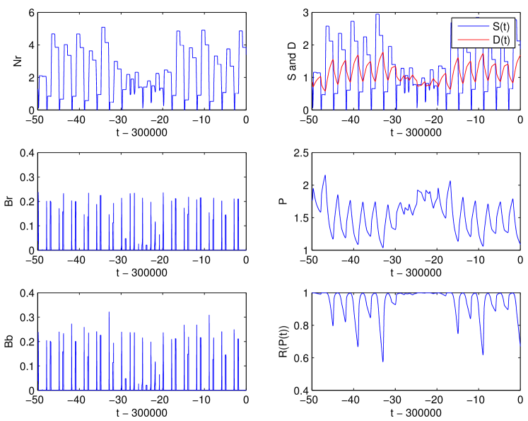
Figure 1. Continuous time dynamics for setting SP over 50 years: $N_{r}$ (top left), $S$ and $D$ (top right), $B_{r}$ (middle left), $P$ (middle right), $B_{b}$ (bottom left) and $R(P)$ (bottom right).

The continuous time dynamics of setting SP can be visualized on Figure 1 over 50 years. Note that on Figure 1 the mature reproducing population $N_{r}(t)$ goes through very small values, of order $10^{-3}$, which might seem unrealistic. This phenomenon can be interpreted as follows. There is no mortality, except for animals reaching the maximal ages $A_{1}$ and $\Omega_{1}$. So, if most of the mature reproducing population $N_{r}$ was born during a short period of time, $N_{r}(t)$ will drop down to (almost) zero $A_{1}$ years later. Here, we observe such drops, which do not endanger the whole population because it holds during the reproducing season and it doesn’t occur too fast (the reproducing females were not all born during a too short time period). Therefore, once the drop has started, as soon as $N_{r}$ goes below 1, a large number of birth will happen, leading to mature reproducing females after a time delay $A_{0}$. So, even if $N_{r}$ was going exactly to zero during this delay period, it would increase again as soon as the newborn females become mature.

A good way to visualize this phenomenon is given by Figure 2 where $N_{r}(t)$ is plotted (left) together with the totale female population in the reproducing line (right): the latter quantity never goes below $0.4$.

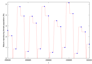
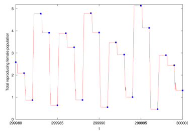
Figure 2. Setting SP, continuous time dynamics of reproducing female population over 20 years: mature ($N_{r}$, left) and total population (right).

A similar phenomenon holds with the butchery line (see Figure 3), where the “mature” butchery population (proportional to the supply $S(t)$) goes close to zero (left) but not the total butchery population (right).

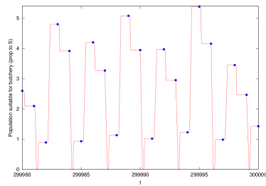
Figure 3. Setting SP, continuous time dynamics of butchery population over 20 years: “mature” ($\propto S$, left) and total population (right).

5.2.2. Yearly dynamics

A natural way to display the behavior of the dynamical system we are studying is to only look at the values it takes for $t\in\mathbb{N}$, that is, at the very beginning of the birth period. We recall that the continuous time dynamics takes place in an infinite-dimensional space $\mathcal{X}$ corresponding to couples of functions $(N(t),P(t))$, where $t$ varies in some interval. Our discretization (see Appendix A) leads to a discrete dynamical system in a phase space of dimension $2\times 201$. Then, we can visualize the dynamics by plotting in $\mathbb{R}^{3}$ the set $\left\{\left.(N_{r}(t),N_{r}(t+1),N_{r}(t+2))\,,\,t\in\mathbb{N}\right.\right\}$, as shown by Figure 4, or the set $\left\{\left.(P(t),P(t+1),P(t+2))\,,\,t\in\mathbb{N}\right.\right\}$, as shown by Figure 5. Both figures are the projection of the same attractor on two different subspaces. We estimate the fractal dimension of the first set to $1.52$ and of the second one to $1.84$. It seems reasonable to conjecture the existence of a strange attractor of dimension $d\in(1,2)$. See Section A.4, Figure 12 and Figure 13, for details on how we estimate the fractal dimension. Note that Figure 4 shows an attractor similar to the one of the Yoccoz-Birkeland model with $\rho=0.30$, $\gamma=8.25$, $A_{0}=0.18$ and $m_{0}=50$ [Arl04, Figure 12]; only the center of the attractor here seems more complex. On the other hand, the interaction between the population and the price equation is crucial, as shown by Section 5.2.3 below.

Figure 4. 3d plot of $(N_{r}(t),N_{r}(t+1),N_{r}(t+2))$ with $t\in\mathbb{N}$, $280\,000\leq t\leq 300\,000$ for setting SP.

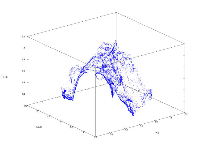
Figure 5. 3d plot of $(P(t),P(t+1),P(t+2))$, with $t\in\mathbb{N}$, $280\,000\leq t\leq 300\,000$ for setting SP.

5.2.3. Comparison with setting SP₁: SP with $R$ constant

Let us call SP₁ the setting SP with the value of the fraction of reproducing females in (3.8a) freezed: $R(P)=R_{\mathrm{cst}}\approx 0.955$ for all $P>0$. The constant value taken for $R$ is equal to the empirical average of $R(P(t))$ in setting SP for $t\in[290\,000,300\,000]$. So, comparing results obtained with SP₁ and SP shows the effect of the coupling between price and population. Note also that setting SP₁ then is an instance of the Yoccoz-Birkeland model with $A_{0}=0.18$, $A_{1}=2$, $\gamma=8.25$ and $m_{0}\approx 4.78$ (with slightly different functions $m$ and $m_{\rho}$, compared to [Arl04]).

The yearly dynamics of setting SP₁ can be visualized on Figure 6 for $95\,000\leq t\leq 100\,000$: it exihibits only a low-complexity seemingly nonchaotic orbit, very close to being periodic and totally different also from the original Yoccoz-Birkeland attractor.

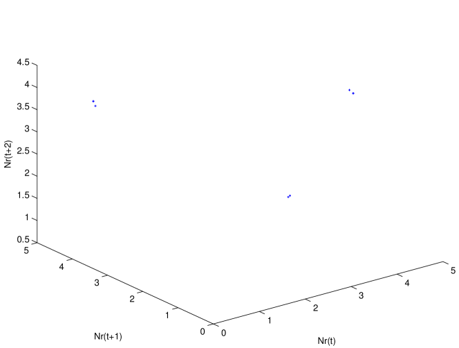
Figure 6. 3d plot of $(N_{r}(t),N_{r}(t+1),N_{r}(t+2))$, with $t\in\mathbb{N}$, $95\,000\leq t\leq 100\,000$ for setting SP₁.

5.2.4. Analysis of chaos

In order to analyze the chaoticity of the dynamics of the price $P$, we followed a time series approach as in [KS03]: we computed the autocorrelation function and determined its first zero $\tau^{*}$. Then we sampled the price time series at time steps multiple of $\tau^{*}$ and we computed the combinatorial entropy for the binary sequence obtained by looking at the sign of price returns (see Figure 7).

Given a times series $(Y(t))_{t\geq 0}$, its autocorrelation function is defined by

$$\forall\tau>0\,,\quad R_{Y}(\tau):=\frac{\Bigl{\langle}\bigl{(}Y-\left\langle Y\right\rangle\bigr{)}\Bigl{(}Y(\cdot+\tau)-\bigl{\langle}Y(\cdot+\tau)\bigr{\rangle}\Bigr{)}\Bigr{\rangle}}{\sqrt{\Bigl{\langle}\bigl{(}Y-\left\langle Y\right\rangle\bigr{)}^{2}\Bigr{\rangle}\left\langle\Bigl{(}Y(\cdot+\tau)-\bigl{\langle}Y(\cdot+\tau)\bigr{\rangle}\Bigr{)}^{2}\right\rangle}}\enspace,$$

where $\left\langle\cdot\right\rangle$ means an average over time. In other words, the autocorrelation $R_{Y}(\tau)$ is the correlation between $Y(t)$ and $Y(t+\tau)$ for a random $t$ chosen uniformly in $[0,T]$, for some large time window $T>0$. So, roughly speaking, $R_{Y}(\tau)$ close to 0 means that $Y(t)$ does not provide information for predicting $Y(t+\tau)$.

The autocorrelation function of $(P(t))_{t\geq 0}$ is plotted on the top left of Figure 7. Its absolute value tends to be smaller for larger values of $\tau$, and it crosses zero several times, first for $\tau=\tau^{\star}\approx 1.37$. Therefore, the discrete dynamical system $(P(k\tau^{\star}))_{k\in\mathbb{N}}$ is a good candidate for being unpredictable. So, we consider the corresponding “returns”

$$r_{k}:=\log_{10}P\bigl{(}(k+1)\tau^{\star}\bigr{)}-\log_{10}P(k\tau^{\star})$$

(which are plotted on the top middle graph of Figure 7), and evaluate the combinatorial entropy $H_{K}$ of the binary sequence $((\operatorname{sign}(r_{i}))_{k-K+1\leq i\leq k})_{k\in\mathbb{N}}$ for various values of $K$ .

The top right plot of Figure 7 shows $H_{K}$ as a function of $K$: there is a clear linear trend, with a positive slope $0.611$ (correlation coefficient $0.995$), which suggests a positive entropy.

We also tried the same analysis for the discrete dynamical system $(P(k))_{k\in\mathbb{N}}$, that is, the time series at integer times, for which the autocorrelation function is not estimated to be (almost) zero. The results are given on the bottom part of Figure 7, with the corresponding returns (middle) and entropy $H_{K}$ as a function of $K$ (right): linear regression still suggests a linear trend with a positive slope $0.647$ (correlation coefficient $0.983$), even if the returns seem less unpredictable as with $\tau^{\star}$ time steps.

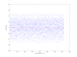
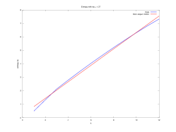
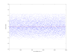
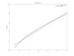
Figure 7. Analysis of chaos for $P$ in setting SP. Top left: autocorrelation function. Its first (approximate) zero is at $\tau^{\star}=1.37$. Middle: sequence of the returns $r_{k}(\tau)=\log_{10}P((k+1)\tau)-\log_{10}P(k\tau)$ for $\tau=\tau^{\star}$ (top) and $\tau=1$ (bottom). Right: estimated entropy $H_{K}$ as a function of $K$, with $\tau=\tau^{\star}$ (top; slope $0.611$ and correlation coefficient $0.995$) and $\tau=1$ (bottom; slope $0.647$ and correlation coefficient $0.983$). See Section 5.2.4 and Appendix A.3 for details.

5.3. Exploration of the parameter space

Starting from setting SP, we changed the parameters one by one between $\gamma$ and $m_{0}$. The resulting bifurcation diagrams are shown on Figures 8 and 10, for $N_{r}$ and Figures 9 and 11, for $P$. Appendix A.5 provides details about how the bifurcation diagrams have been obtained.

5.3.1. Setting SP with $\gamma$ varying

A bifurcation diagram is plot on Figure 8, showing $\left\{\left.N_{r}(t),t\in\mathbb{N}\right.\right\}$ as a function of $\gamma\in[2,10]$. A corresponding bifurcation diagram for the price $P$ is shown on Figure 9. The dynamics look like complex for the largest part of the interval, with only few and very small windows of periodicity. In particular, chaotic behavior seems to arise also for small values of $\gamma$ (i.e. when the fertility rate $m(N)$ depends in a weaker way on the population $N$) which are probably more reasonable in a human-controlled breeding facility.

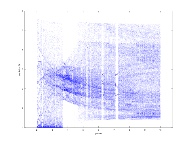
Figure 8. Bifurcation diagram for $N_{r}(t)$ w.r.t. $\gamma\in[2,10]$ around setting SP.

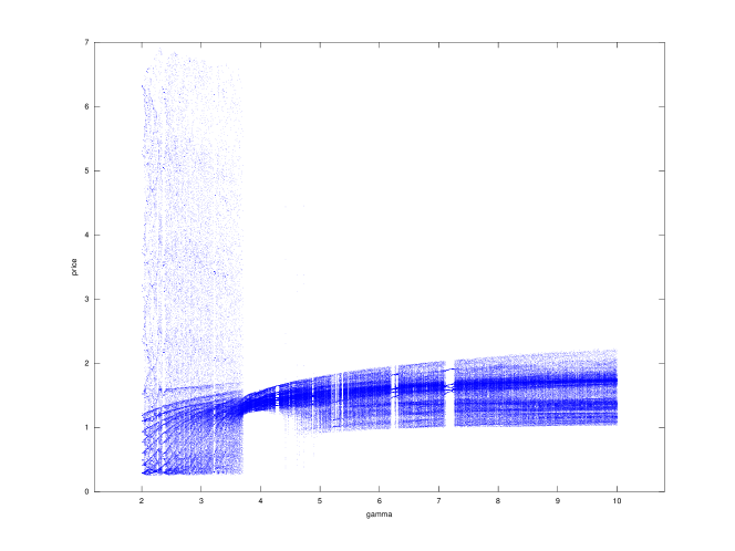
Figure 9. Bifurcation diagram for $P(t)$ w.r.t. $\gamma\in[2,10]$ around setting SP.

5.3.2. Setting SP with $m_{0}$ varying

A bifurcation diagram is plot on Figure 10, showing $\left\{\left.N_{r}(t),t\in\mathbb{N}\right.\right\}$ as a function of $m_{0}\in[2,8]$. The corresponding bifurcation diagram for the price $P$ is shown on Figure 11. Here period doubling cascades seem to arise in the windows of periodicity. Moreover, at a closer inspection of Figures 10 and 11, a relatively small amplitude Hopf bifurcation seems to happen near $m_{0}\approx 5.4$.

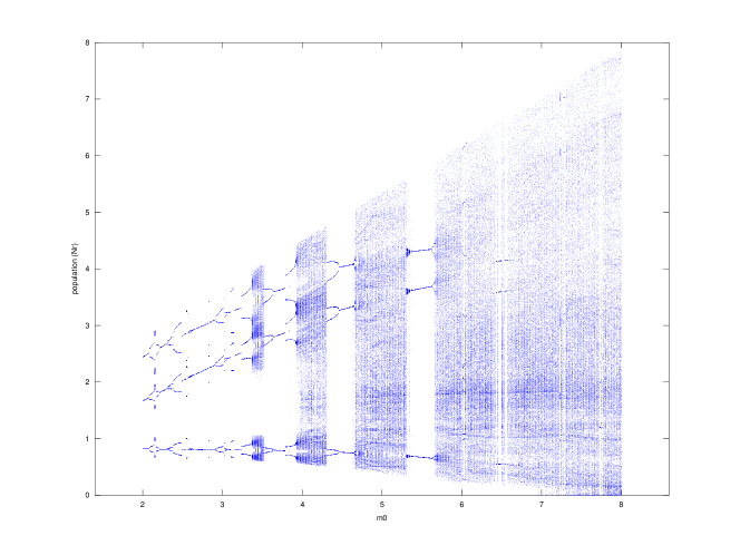
Figure 10. Bifurcation diagram for $N_{r}(t)$ w.r.t. $m_{0}\in[2,8]$ around setting SP.

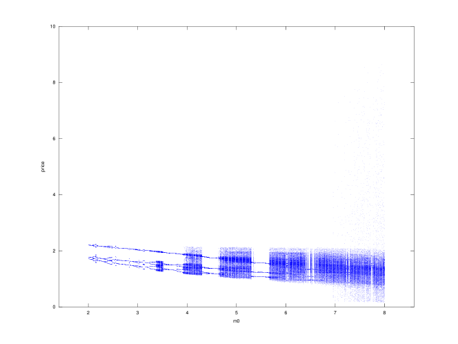
Figure 11. Bifurcation diagram for $P(t)$ w.r.t. $m_{0}\in[2,8]$ around setting SP.

Appendix A Technical details about the simulations

This section provides all technical details necessary to reproduce our numerical experiments.

A.1. Discretization of the model

Throughout the paper, we consider the following discretization with $q=100$ steps per year. This will lead to a deterministic dynamical system in a phase space of dimension $2\times 201$.

A.1.1. Notation and parameters

We replace the continous time parameter $t\in[0,+\infty)$ by indices $i\in\mathbb{N}\backslash\left\{\left.0\right.\right\}$.
Roughly, $i\geq 1$ replaces the interval $\left(\frac{i-1}{q},\frac{i}{q}\right]$ where $q\geq 1$ is an integer (number of steps per year).

• $q\in\mathbb{N}\backslash\left\{\left.0\right.\right\}$ is the number of steps per year

• $N_{r,i}$ approximates the average of $N_{r}(t)$ over $t\in\left(\frac{i-1}{q},\frac{i}{q}\right]$:

  $$N_{r,i}\approx q\int_{\frac{i-1}{q}}^{\frac{i}{q}}N_{r}(t)dt$$

• Similarly, $N_{b,i}$, $m_{\rho,i}$, $S_{i}$ and $P_{i}$ are respectively defined from $N_{b}(t)$, $m_{\rho}(t)$, $S(t)$ and $P(t)$.

• $B_{r,i}$ approximates the number of newborn females put in the reproducing line in the interval $t\in\left(\frac{i-1}{q},\frac{i}{q}\right]$:

  $$B_{r,i}\approx\int_{\frac{i-1}{q}}^{\frac{i}{q}}B_{r}(t)dt$$

  Note the difference with $N_{r}$ coming from the fact $B_{r}(t)$ is a density (number per unit of time) contrary to $N_{r}(t)$ that is a number of individuals.
  Similarly, $B_{b,i}$, $B_{f,i}$, $B_{m,i}$ are defined respectively from $B_{b}(t)$, $B_{f}(t)$, $B_{m}(t)$.

We also need to discretize some of the model parameters (with a few technical modifications in order to avoid some troubles):

• $k_{A_{0}}=\max\left\{\left.1,\left[\left.qA_{0}\right.\right]\right.\right\}$ where $\left[\left.x\right.\right]$ is the closest integer to $x$. We want $k_{A_{0}}>0$ so that $N_{r,k}$ only depends on the past of $B_{r}$ in (A.1), otherwise we would have a circular definition.

• $k_{A_{1}}=\max\left\{\left.k_{A_{0}},\left[\left.qA_{1}\right.\right]-1\right.\right\}$. We want $k_{A_{1}}\geq k_{A_{0}}$ in order to make the sum (A.1) non-empty when $A_{0}=A_{1}$. We take $\left[\left.qA_{1}\right.\right]-1$ instead of $\left[\left.qA_{1}\right.\right]$ because animals are supposed to die exactly at age $A_{1}$, so individual of age $A_{1}$ at time $k/q$ (counted in $B_{r,k-\left[\left.qA_{1}\right.\right]}$) do not count in $N_{r,k}$.

• $k_{\Omega_{0}}=\max\left\{\left.1,\left[\left.q\Omega_{0}\right.\right]\right.\right\}$ (similarly to $k_{A_{0}}$)

• $k_{\Omega_{1}}=\max\left\{\left.k_{\Omega_{0}},\left[\left.q\Omega_{1}\right.\right]-1\right.\right\}$ (similarly to $k_{A_{1}}$)

A.1.2. Discretized model

At any time step $k\geq 1$, we compute

$$Z_{k}:=(N_{r,k}\,;\,N_{b,k}\,;\,S_{k}\,;\,P_{k}\,;\,B_{r,k}\,;\,B_{b,k})$$

from its past values

$$\left(\left.Z_{i}\right.\right)_{k-\max\{k_{A_{1}},k_{\Omega_{1}}\}\leq i\leq k-1}\enspace,$$

in the following order:

(A.1) $$N_{r,k} =\sum_{j=k_{A_{0}}}^{k_{A_{1}}}B_{r,k-j}$$

(A.2) $$N_{b,k} =\sum_{j=k_{\Omega_{0}}}^{k_{\Omega_{1}}}B_{b,k-j}$$

(A.3) $$S_{k} =\frac{qN_{b,k}}{k_{\Omega_{1}}-k_{\Omega_{0}}+1}$$

(A.4) $$P_{k} =\max\left\{\left.0,P_{k-1}+\frac{\lambda P_{k-1}F\bigl{(}D(P_{k-1}),S_{k}\bigr{)}}{q}\right.\right\}$$

(A.5) $$B_{r,k} =\frac{m_{0}}{q}m_{\rho,k}m(N_{r,k})R(P_{k})$$

(A.6) $$B_{b,k} =\frac{m_{0}}{q}m_{\rho,k}m(N_{r,k})\bigl{(}2-R(P_{k})\bigr{)}$$

A.2. Initial condition

The initial condition is given by the values of the number of newborns ($B_{r,i}$ and $B_{b,i}$) for time steps $i=1,\ldots,k_{A_{1}}$ before the start of the simulation, since the discretized model above (Eq. (A.1)–(A.6)) only needs the past values of $B_{r}$ and $B_{b}$ to compute the future dynamics of the model.

For each parameter set, we choose an initial condition randomly (but with a known random seed, so we can use repeatedly the same initial condition to obtain our bifurcation diagrams, for instance) as follows: $B_{r,1},\ldots,B_{r,k_{A_{1}}},B_{b,1},\ldots,B_{b,k_{A_{1}}}$ are chosen independent with common distribution $\mathcal{U}\left(\left.\left[\left.0,\frac{2}{k_{A_{1}}-k_{A_{0}}+1}\right.\right]\right.\right)$. The reason for this choice is that $k_{A_{1}}-k_{A_{0}}+1$ is the number of time steps corresponding to reproducing ages of females. So, for instance, by Eq. (A.1), the reproducing female population at time $k_{A_{1}}+1$ is the average of random variables uniform over $[0,2]$, so it should be close to 1, the threshold value for density-dependence to apply.

A.3. Chaos analysis

In each setting and for each time series $Y\in\left\{\left.N_{r},P\right.\right\}$, we start from the “continuous” time series of $Y(t)$ for $t>T_{\max}-10\,000$, where $T_{\max}$ is the total length of the simulation experiment (i.e., $T_{\max}=300\,000$ for setting SP, and $T_{\max}=100\,000$ for other settings). Then, we compute the empirical autocorrelation function of $Y$ with lags $\tau\in[0,100]$ ($\tau$ is expressed in years). We get its first “zero” $\tau^{\star}$ as the first point where the empirical autocorrelation crosses zero, and we then check that the value of the empirical autocorrelation at $\tau=\tau^{\star}$ is smaller than an arbitrary threshold (here, $10^{-2}$); this holds true in all the settings where we did such an analysis.

Then, we consider the sequence $Y(t)$ only at times $t$ equal to an integer multiple of $\tau^{\star}$, and compute the returns $\log_{10}(Y((i+1)\tau^{\star})/Y(i\tau^{\star}))$ and their respective signs $\varepsilon_{i}\in\left\{\left.-1,1\right.\right\}$. From this (finite) sequence of signs, we compute for $K=1,\ldots,12$ the combinatorial entropy $H_{K}(\tau^{\star})$ of $((\varepsilon_{i})_{k-K+1\leq i\leq k})_{k\in\mathbb{N}}$:

$$H_{K}(\tau^{\star}):=-\sum_{x\in\left\{\left.-1,1\right.\right\}^{K}}p_{x}\log_{2}(p_{x})\qquad\mbox{where}\quad p_{x}=\mathbb{P}\bigl{(}(\varepsilon_{i})_{k-K+1\leq i\leq k}=x\bigr{)}$$

the latter probability being with respect to $k$.

Finally, we plot $H_{K}(\tau^{\star})$ as a function of $K$ and perform a standard robust linear regression in order to estimate its slope.

We also do the same analysis when considering $Y(t)$ at integer times, leading to a plot of $H_{K}(1)$ as a function of $K$, on which we estimate its slope by performing a standard robust linear regression.

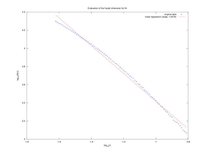
Figure 12. Estimation of the fractal dimension of the attractor of Figure 4 (setting SP, $N_{r}$).

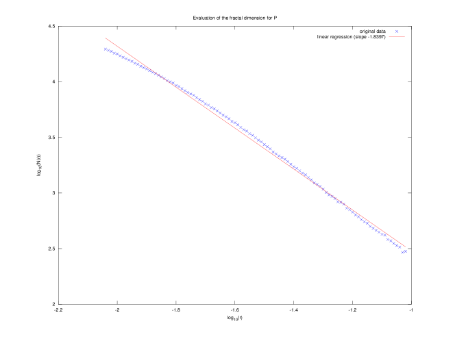
Figure 13. Estimation of the fractal dimension of the attractor of Figure 5 (setting SP, $P$).

A.4. Fractal dimension

For computing the fractal dimension of the attractors for setting SP, we started from their 3-dimensional visualization over $200\,000$ years, that is, for $N_{r}$ for instance:

$$\mathcal{K}=\Bigl{\{}\bigl{(}N_{r}(t),N_{r}(t+1),N_{r}(t+2)\bigr{)}\,,\,100\,000\leq t\leq 300\,000\Bigr{\}}\enspace.$$

Then, for various values of $\epsilon>0$, we compute the number $\widetilde{\mathcal{N}}_{\epsilon}(\mathcal{K})$ of cubes $\mathcal{C}_{i,j,k}=[i\epsilon;(i+1)\epsilon]\times[j\epsilon;(j+1)\epsilon]\times[k\epsilon;(k+1)\epsilon]$ that contain at least one point of $\mathcal{K}$. Figure 12 thus represents $\log_{10}\widetilde{\mathcal{N}}_{\epsilon}(\mathcal{K})$ as a function of $\log_{10}\epsilon$.

Theoretically, the fractal dimension is the opposite of the slope of this graph at infinity. Here, since $\mathcal{K}$ is finite, $\widetilde{\mathcal{N}}_{\epsilon}(\mathcal{K})$ is constant equal to $\operatorname{Card}(\mathcal{K})$ for small $\epsilon$. So, we estimated the slope of the graph only for a limited set of values of $\epsilon$. One can check on Figure 12 that the linear fit seems reasonably close to the original curve.

Because of the numerous approximations made during this estimation, the precise value of the fractal dimension should not be taken into account too seriously, but its order of magnitude should be correct. Figure 13 shows the corresponding estimation with $P$ instead of $N_{r}$.

A.5. Bifurcation diagrams

We took the same initial condition for all settings in all diagrams (by choosing a fixed arbitrary seed to the random number generator). Then, for each value of the parameter we plot the sequence of values of $N_{r}(t)$ (resp. $P(t)$) for $t\in\left\{\left.1\,500,\ldots,2\,000\right.\right\}$. In all diagrams, the parameters are varying by step of $0.01$.

References

- [AMMY18] Sylvain Arlot, Stefano Marmi, Carlos Matheus, and Nigel Gilles Yoccoz. Dynamique de populations de petits mammifères, saisonnalité et attracteur de Hénon – comment une question d’écologie a pu intéresser Jean-Christophe. Gazette des mathématiciens, Numéro spécial Jean-Christophe Yoccoz, 6–14, April 2018.
- [Arl04] Sylvain Arlot. Étude d’un modèle de dynamique des populations. Technical Report 2004-38, University Paris-Sud 11 Orsay, September 2004. arXiv:1204.0799 Master thesis. Advisor: Jean-Christophe Yoccoz.
- [BM89] Jacques Bélair and Michael C. Mackey. Consumer memory and price fluctuations in commodity markets: an integrodifferential model. J. Dynam. Differential Equations, 1(3):299–325, 1989.
- [Cam09] Gustavo Campodoni. I sistemi di allevamento. Il bosco e l’allevamento della razza Cinta Senese, ARSIA:121–166, 2009.
- [Chi88] C. Chiarella. The cobweb model: its instability and the onset of chaos. Economic Modelling, 5(4):377–384, 1988.
- [Eze38] Mordecai Ezekiel. The cobweb theorem. The Quarterly Journal of Economics, 52(2):255–280, 1938.
- [FP07] Oreste Franci and Caterina Pugliese. Italian autochthonous pigs: progress report and research perspectives. Ital. J. Anim. Sci., 6:663–671, 2007.
- [GM86] J.-M. Grandmont and P. Malgrange. Nonlinear economics dynamics: Introduction. Journal of Economic Theory, 40(1):3–12, 1986.
- [Han28] Arthur Hanau. Die Prognose der Schweinepreise. PhD dissertation, In: Vierteljahreshefte zur Konjunkturforschung, Verlag Reimar Hobbing, Berlin., 1928.
- [Har64] Philip Hartman. Ordinary Differential Equations. John Wiley and Sons, Inc., 1964.
- [Hom94] C. Hommes. Dynamics of the cobweb model with adaptive expectations and nonlinear suppy and demand. Journal of Economic Behavior and Organization, 24:315–335, 1994.
- [Hom13] Cars Hommes. Behavioral Rationality and Heterogeneous Expectations in Complex Economic Systems. Cambridge University Press, 2013.
- [HS87] Dermot J. Hayes and Andrew Schmitz. Hog cycles and countercyclical production response. American Journal of Agricultural Economics, 69(4):762–770, 1987.
- [KH13] Mark T. Knauer and Chris E. Hostetler. Us swine industry productivity analysis, 2005 to 2010. J. Swine Health Prod., 21:248–252, 2013.
- [KS03] Holger Kantz and Thomas Schreider. Nonlinear Time Series Analysis. Cambridge University Press, 2003.
- [Mac89] Michael C. Mackey. Commodity price fluctuations: price dependent delays and nonlinearities as explanatory factors. J. Econom. Theory, 48(2):497–509, 1989.
- [NPV12] Juan José Nieto, Maria José Pacifico, and José Ladislau Vieitez. Long-Term and Short-Term Dynamics of Microtus epiroticus: A Yoccoz–Birkeland Model. SIAM J. Appl. Dyn. Syst., 11(4): 1499–1532, 2012.
- [RMS94] S. Rosen, K.M. Murphy, and J.A. Scheinkman. Cattle cycles. The Journal of Political Economy, 102(3):468–492, 1994.
- [Sor79] Anton Marinus Sorensen. Animal Reproduction, Principles and Practices. McGraw-Hill, 1979.
- [YB98] Jean-Christophe Yoccoz and H. Birkeland. Informal commentaries on the numerical investigation of the toy model. September 1998.
- [YI99] Nigel G. Yoccoz and Rolf A. Ims. Demography of small mammals in cold regions: the importance of environmental variability. Ecological Bulletins, 47:133–144, 1999.
- [Zan09] Nicola Zanda. Personal communication, 2009.