Redundancy Techniques for Straggler Mitigation in Distributed Optimization and Learning

Abstract

Performance of distributed optimization and learning systems is bottlenecked by “straggler” nodes and slow communication links, which significantly delay computation. We propose a distributed optimization framework where the dataset is “encoded” to have an over-complete representation with built-in redundancy, and the straggling nodes in the system are dynamically left out of the computation at every iteration, whose loss is compensated by the embedded redundancy. We show that oblivious application of several popular optimization algorithms on encoded data, including gradient descent, L-BFGS, proximal gradient under data parallelism, and coordinate descent under model parallelism, converge to either approximate or exact solutions of the original problem when stragglers are treated as erasures. These convergence results are deterministic, i.e., they establish sample path convergence for arbitrary sequences of delay patterns or distributions on the nodes, and are independent of the tail behavior of the delay distribution. We demonstrate that equiangular tight frames have desirable properties as encoding matrices, and propose efficient mechanisms for encoding large-scale data. We implement the proposed technique on Amazon EC2 clusters, and demonstrate its performance over several learning problems, including matrix factorization, LASSO, ridge regression and logistic regression, and compare the proposed method with uncoded, asynchronous, and data replication strategies.

Keywords: Distributed optimization, straggler mitigation, proximal gradient, coordinate descent, restricted isometry property

1 Introduction

Solving learning and optimization problems at present scale often requires parallel and distributed implementations to deal with otherwise infeasible computational and memory requirements. However, such distributed implementations often suffer from system-level issues such as slow communication and unbalanced computational nodes. The runtime of many distributed implementations are therefore throttled by that of a few slow nodes, called stragglers, or a few slow communication links, whose delays significantly encumber the overall learning task. In this paper, we propose a distributed optimization framework based on proceeding with each iteration without waiting for the stragglers, and encoding the dataset across nodes to add redundancy in the system in order to mitigate the resulting potential performance degradation due to lost updates.

We consider the master-worker architecture, where the dataset is distributed across a set of worker nodes, which directly communicate to a master node to optimize a global objective. The encoding framework consists of an efficient linear transformation (coding) of the dataset that results in an overcomplete representation, which is then partitioned and distributed across the worker nodes. The distributed optimization algorithm is then performed directly on the encoded data, with all worker nodes oblivious to the encoding scheme, i.e., no explicit decoding of the data is performed, and nodes simply solve the effective optimization problem after encoding. In order to mitigate the effect of stragglers, in each iteration, the master node only waits for the first $k$ updates to arrive from the $m$ worker nodes (where $k\leq m$ is a design parameter) before moving on; the remaining $m-k$ node results are effectively erasures, whose loss is compensated by the data encoding.

The framework is applicable to both the data parallelism and model parallelism paradigms of distributed learning, and can be applied to distributed implementations of several popular optimization algorithms, including gradient descent, limited-memory-BFGS, proximal gradient, and block coordinate descent. We show that if the linear transformation is designed to satisfy a spectral condition resembling the restricted isometry property, the iterates resulting from the encoded version of these algorithms deterministically converge to an exact solution for the case of model paralellism, and an approximate one under data parallelism, where the approximation quality only depends on the properties of encoding and the parameter $k$. These convergence guarantees are deterministic in the sense that they hold for any pattern of node delays, i.e., even if an adversary chooses which nodes to delay at every iteration. In addition, the convergence behavior is independent of the tail behavior of the node delay distribution. Such a worst-case guarantee is not possible for the asynchronous versions of these algorithms, whose convergence rates deteriorate with increasing node delays. We point out that our approach is particularly suited to computing networks with a high degree of variability and unpredictability, where a large number of nodes can delay their computations for arbitrarily long periods of time.

Our contributions are as follows: (i) We propose the encoded distributed optimization framework, and prove deterministic convergence guarantees under this framework for gradient descent, L-BFGS, proximal gradient and block coordinate descent algorithms; (ii) we provide three classes of encoding matrices, and discuss their properties, and describe how to efficiently encode with such matrices on large-scale data; (iii) we implement the proposed technique on Amazon EC2 clusters and compare their performance to uncoded, replication, and asynchronous strategies for problems such as ridge regression, collaborative filtering, logistic regression, and LASSO. In these tasks we show that in the presence of stragglers, the technique can result in significant speed-ups (specific amounts depend on the underlying system, and examples are provided in Section 5) compared to the uncoded case when all workers are waited for in each iteration, to achieve the same test error.

Related work.

The approaches to mitigating the effect of stragglers can be broadly classified into three categories: replication-based techniques, asynchronous optimization, and coding-based techniques.

Replication-based techniques consist of either re-launching a certain task if it is delayed, or pre-emptively assigning each task to multiple nodes and moving on with the copy that completes first. Such techniques have been proposed and analyzed in Gardner et al. (2015); Ananthanarayanan et al. (2013); Shah et al. (2016); Wang et al. (2015); Yadwadkar et al. (2016), among others. Our framework does not preclude the use of such system-level strategies, which can still be built on top of our encoded framework to add another layer of robustness against stragglers. However, it is not possible to achieve the worst-case guarantees provided by encoding with such schemes, since it is still possible for both replicas to be delayed.

Perhaps the most popular approach in distributed learning to address the straggler problem is asynchronous optimization, where each worker node asynchronously pushes updates to and fetches iterates from a parameter server independently of other workers, hence the stragglers do not hold up the entire computation. This approach was studied in Recht et al. (2011); Agarwal and Duchi (2011); Dean et al. (2012); Li et al. (2014) (among many others) for the case of data parallelism, and Liu et al. (2015); You et al. (2016); Peng et al. (2016); Sun et al. (2017) for coordinate descent methods (model parallelism). Although this approach has been largely successful, all asynchronous convergence results depend on either a hard bound on the allowable delays on the updates, or a bound on the moments of the delay distribution, and the resulting convergence rates explicitly depend on such bounds. In contrast, our framework allows for completely unbounded delays. Further, as in the case of replication, one can still consider asynchronous strategies on top of the encoding, although we do not focus on such techniques within the scope of this paper.

A more recent line of work that address the straggler problem is based on coding-theory-inspired techniques Tandon et al. (2017); Lee et al. (2016); Dutta et al. (2016); Karakus et al. (2017a, b); Yang et al. (2017); Halbawi et al. (2017); Reisizadeh et al. (2017). Some of these works focus exclusively on coding for distributed linear operations, which are considerably simpler to handle. The works in Tandon et al. (2017); Halbawi et al. (2017) propose coding techniques for distributed gradient descent that can be applied more generally. However, the approach proposed in these works require a redundancy factor of $r+1$ in the code, to mitigate $r$ stragglers. Our approach relaxes the exact gradient recovery requirement of these works, consequently reducing the amount of redundancy required by the code.

The proposed technique, especially under data parallelism, is also closely related to randomized linear algebra and sketching techniques in Mahoney et al. (2011); Drineas et al. (2011); Pilanci and Wainwright (2015), used for dimensionality reduction of large convex optimization problems. The main difference between this literature and the proposed coding technique is that the former focuses on reducing the problem dimensions to lighten the computational load, whereas encoding increases the dimensionality of the problem to provide robustness. As a result of the increased dimensions, coding can provide a much closer approximation to the original solution compared to sketching techniques. In addition, unlike these works, our model allows for an arbitrary convex regularizer in addition to the encoded loss term.

2 Encoded Distributed Optimization

We will use the notation $[j]=\left\{i\in\mathbb{Z}:1\leq i\leq j\right\}$. All vector norms refer to 2-norm, and all matrix norms refer to spectral norm, unless otherwise noted. The superscript ^c will refer to complement of a subset, i.e., for $A\subseteq[m]$, $A^{c}=[m]\backslash A$. For a sequence of matrices $\left\{M_{i}\right\}$ and a set $A$ of indices, we will denote $\left[M_{i}\right]_{i\in A}$ to mean the matrix formed by stacking the matrices $M_{i}$ vertically. The main notation used throughout the paper is provided in Table 1.

We consider a distributed computing network where the dataset $\left\{\left(x_{i},y_{i}\right)\right\}_{i=1}^{n}$ is stored across a set of $m$ worker nodes, which directly communicate with a single master node. In practice the master node can be implemented using a fully-connected set of nodes, but this can still be abstracted as a single master node.

It is useful to distinguish between two paradigms of distributed learning and optimization; namely, data parallelism, where the dataset is partitioned across data samples, and model parallelism, where it is partitioned across features (see Figures 2 and 4). We will describe these two models in detail next.

Notation	Explanation
$[j]$	The set $\left\{i\in\mathbb{Z}:1\leq i\leq j\right\}$
$m$	Number of worker nodes
$n,p$	The dimensions of the data matrix $X\in\mathbb{R}^{n\times p}$, vector $y\in\mathbb{R}^{n\times 1}$
$k_{t}$	Number of updates the master node waits for in iteration $t$, before moving on
$\eta_{t}$	Fraction of nodes waited for in iteration, i.e., $\eta_{t}=\frac{k_{t}}{m}$
$A_{t}$	The subset of nodes $[m]$ which send the fastest $k_{t}$ updates at iteration $t$
$f(w),\widetilde{f}(w)$	The original and encoded objectives, respectively, under data parallelism
$g(w)=\phi(Xw)$	The original objective under model parallelism
$\widetilde{g}(v)=\phi(XS^{\top}v)$	The encoded objective under model parallelism
$h(w)$	Regularization function (potentially non-smooth)
$\nu$	Strong convexity parameter
$L$	Smoothness parameter for $h(w)$ (if smooth), and $g(w)$
$\lambda$	Regularization parameter
$\Psi_{t}$	Mapping from gradient updates to step $\left\{\nabla f_{i}(t)\right\}_{i\in A_{t}}\mapsto d_{t}$
$d_{t}$	Descent direction chosen by the algorithm
$\alpha_{t}$, $\alpha$	Step size
$M,\mu$	Largest and smallest eigenvalues of $X^{\top}X$, respectively
$\beta$	Redundancy factor ($\beta\geq 1$)
$S$	Encoding matrix with dimensions $\beta n\times n$
$S_{i}$	$i$th row-block of $S$, corresponding to worker $i$
$S_{A}$	Submatrix of $S$ formed by $\left\{S_{i}\right\}_{i\in A\subseteq[m]}$ stacked vertically

Table 1: Notation used in the paper.

Figure 1: Uncoded distributed optimization with data parallelism, where $X$ and $y$ are partitioned as $X=\left[X_{i}\right]_{i\in[m]}$ and $y=\left[y_{i}\right]_{i\in[m]}$.

Figure 2: Encoded setup with data parallelism, where node $i$ stores $\left(S_{i}X,S_{i}y\right)$, instead of $\left(X_{i},y_{i}\right)$. The uncoded case corresponds to $S=I$.

2.1 Data parallelism

We focus on objectives of the form

$$f(w)=\frac{1}{2n}\|Xw-y\|^{2}+\lambda h(w),$$ (1)

where $X$ and $y$ are the data matrix and data vector, respectively. We assume each row of $X$ corresponds to a data sample, and the data samples and response variables can be horizontally partitioned as $X=\left[X_{1}^{\top}\;X_{2}^{\top}\;\cdots\;X_{m}^{\top}\right]^{\top}$ and $y=\left[y_{1}^{\top}\;y_{2}^{\top}\;\cdots\;y_{m}^{\top}\right]^{\top}$. In the uncoded setting, machine $i$ stores the row-block $X_{i}$ (Figure 2). We denote the largest and smallest eigenvalues of $X^{\top}X$ with $M>0$, and $\mu\geq 0$, respectively. We assume $\lambda\geq 0$, and $h(w)\geq 0$ is a convex, extended real-valued function of $w$ that does not depend on data. Since $h(w)$ can take the value $h(w)=\infty$, this model covers arbitrary convex constraints on the optimization.

The encoding consists of solving the proxy problem

$$\widetilde{f}(w)=\frac{1}{2n}\|S\left(Xw-y\right)\|^{2}+\lambda h(w)=\frac{1}{2n}\sum_{i=1}^{m}\underbrace{\|S_{i}\left(Xw-y\right)\|^{2}}_{f_{i}(w)}+\lambda h(w),$$ (2)

instead, where $S\in\mathbb{R}^{\beta n\times n}$ is a designed encoding matrix with redundancy factor $\beta\geq 1$, partitioned as $S=\left[S_{1}^{\top}\;S_{2}^{\top}\;\cdots\;S_{m}^{\top}\right]^{\top}$ across $m$ machines. Based on this partition, worker node $i$ stores $\left(S_{i}X,S_{i}y\right)$, and operates to solve the problem (2) in place of (1) (Figure 2). We will denote $\hat{w}\in\operatorname*{arg\,min}\widetilde{f}(w)$, and $w^{*}\in\operatorname*{arg\,min}f(w)$.

In general, the regularizer $h(w)$ can be non-smooth. We will say that $h(w)$ is $L$-smooth if $\nabla h(w)$ exists everywhere and satisfies

$$h(w^{\prime})\leq h(w)+\langle\nabla h(w),w^{\prime}-w\rangle+\frac{L}{2}\|w^{\prime}-w\|^{2}$$

for some $L>0$, for all $w,w^{\prime}$. The objective $f$ is $\nu$-strongly convex if, for all $x,y$,

$$f(y)\geq f(x)+\left\langle\nabla f(x),y-x\right\rangle+\frac{\nu}{2}\|x-y\|^{2}.$$

Once the encoding is done and appropriate data is stored in the nodes, the optimization process works in iterations. At iteration $t$, the master node broadcasts the current iterate $w_{t}$ to the worker nodes, and wait for $k_{t}$ gradient updates $\nabla f_{i}(w)$ to arrive, corresponding to that iteration, and then chooses a step direction $d_{t}$ and a step size $\alpha_{t}$ (based on algorithm $\Psi_{t}$ that maps the set of gradients updates to a step) to update the parameters. We will denote $\eta_{t}=\frac{k_{t}}{m}$. We will also drop the time dependence of $k$ and $\eta$ whenever it is kept constant.

The set of fastest $k_{t}$ nodes to send gradients for iteration $t$ will be denoted as $A_{t}$. Once $k_{t}$ updates have been collected, the remaining nodes, denoted $A_{t}^{c}$, are interrupted by the master node. Algorithms 1 and 2 describe the generic mechanism of the proposed distributed optimization scheme at the master node and a generic worker node, respectively.

The intuition behind the encoding idea is that waiting for only $k_{t}<m$ workers prevents the stragglers from holding up the computation, while the redundancy provided by using a tall matrix $S$ compensates for the information lost by proceeding without the updates from stragglers (the nodes in the subset $A_{t}^{c}$).

We next describe the three specific algorithms that we consider under data parallelism, to compute $d_{t}$.

Gradient descent.

In this case, we assume that $h(w)$ is $L$-smooth. Then we simply set the descent direction

$$d_{t}=-\left(\frac{1}{2n\eta}\sum_{i\in A_{t}}\nabla f_{i}(w_{t})+\lambda\nabla h(w_{t})\right).$$

We keep $k_{t}=k$ constant, chosen based on the number of stragglers in the network, or based on the desired operating regime.

Limited-memory-BFGS.

We assume that $h(w)=\|w\|^{2}$, and assume $\mu+\lambda>0$. Although L-BFGS is traditionally a batch method, requiring updates from all nodes, its stochastic variants have also been proposed by Mokhtari and Ribeiro (2015); Berahas et al. (2016). The key modification to ensure convergence in this case is that the Hessian estimate must be computed via gradient components that are common in two consecutive iterations, i.e., from the nodes in $A_{t}\cap A_{t-1}$. We adapt this technique to our scenario. For $t>0$, define $u_{t}:=w_{t}-w_{t-1}$, and

$$r_{t} :=\frac{m}{2n\left|A_{t}\cap A_{t-1}\right|}\sum_{i\in A_{t}\cap A_{t-1}}\left(\nabla f_{i}(w_{t})-\nabla f_{i}(w_{t-1})\right).$$

Then once the gradient terms $\left\{\nabla f_{i}(w_{t})\right\}_{i\in A_{t}}$ are collected, the descent direction is computed by $d_{t}=-B_{t}\widetilde{g}_{t}$, where $\widetilde{g}_{t}=\frac{1}{2\eta n}\sum_{i\in A_{t}}\nabla f_{i}(w_{t})$, and $B_{t}$ is the inverse Hessian estimate for iteration $t$, which is computed by

$$B_{t}^{(\ell+1)}=V_{j_{\ell,t}}^{\top}B_{t}^{(\ell)}V_{j_{\ell,t}}+\rho_{j_{\ell,t}}u_{j_{\ell,t}}u_{j_{\ell,t}}^{\top},\;\;\;\rho_{j}=\frac{1}{r_{j}^{\top}u_{j}},\;\;\;V_{j}=I-\rho_{j}r_{j}u_{j}^{\top}$$

with $j_{\ell,t}=t-\widetilde{\sigma}+\ell$, $B_{t}^{(0)}=\frac{r_{t}^{\top}r_{t}}{r_{t}^{\top}u_{t}}I$, and $B_{t}:=B_{t}^{(\widetilde{\sigma})}$ with $\widetilde{\sigma}:=\min\left\{t,\sigma\right\}$, where $\sigma$ is the L-BFGS memory length. Once the descent direction $d_{t}$ is computed, the step size is determined through exact line search. To do this, each worker node computes $S_{i}Xd_{t}$, and sends it to the master node. Once again, the master node only waits for the fastest $k_{t}$ nodes, denoted by $D_{t}\subseteq[m]$ (where in general $D_{t}\neq A_{t}$), to compute the step size that minimizes the function along $d_{t}$, given by

$$\alpha_{t}=-\rho\frac{d_{t}^{\top}\widetilde{g}_{t}}{d_{t}^{\top}\widetilde{X}^{\top}_{D}\widetilde{X}_{D}d_{t}},$$ (3)

where $\widetilde{X}_{D}=\left[S_{i}X\right]_{i\in D_{t}}$, and $0<\rho<1$ is a back-off factor of choice.

Proximal gradient.

Here, we consider the general case of non-smooth $h(w)\geq 0,\lambda\geq 0$. The descent direction $d_{t}$ is given by

$$d_{t}=\operatorname*{arg\,min}_{w}\widetilde{F}_{t}(w)-w_{t},$$

where

$$\widetilde{F}_{t}(w) :=\frac{1}{2\eta n}\sum_{i\in A_{t}}f_{i}(w_{t})+\left\langle\frac{1}{2\eta n}\sum_{i\in A_{t}}\nabla f_{i}(w_{t}),w-w_{t}\right\rangle+\lambda h(w)+\frac{1}{2\alpha}\|w-w_{t}\|^{2}.$$

We keep the step size $\alpha_{t}=\alpha$ and $k_{t}=k$ constant.

1: Given: $\Psi_{t}$, a sequence of functions that map gradients $\left\{\nabla f_{i}(w_{t})\right\}_{i\in A_{t}}$ to a descent direction $d_{t}$

2: Initialize $w_{0}$, $\alpha_{0}$

3: for $t=1,\dots,T$ do

4:    broadcast $w_{t}$ to all worker nodes

5:    wait to receive $k_{t}$ gradient updates $\left\{\nabla f_{i}(w_{t})\right\}_{i\in A_{t}}$

6:    send interrupt signal the nodes in $A_{t}^{c}$

7:    compute the descent direction $d_{t}=\Psi_{t}\left(\left\{\nabla f_{i}\left(w_{t}\right)\right\}_{i\in A_{t}}\right)$

8:    determine step size $\alpha_{t}$

9:    take the step $w_{t+1}=w_{t}+\alpha_{t}d_{t}$

10: end for

Algorithm 1 Generic encoded distributed optimization procedure under data parallelism, at the master node.

1: Given: $f_{i}(w)=\|S_{i}(Xw-y)\|^{2}$

2: for $t=1,\dots,T$ do

3:    wait to receive $w_{t}$

4:    while not interrupted by master do

5:       compute $\nabla f_{i}(w_{t})$

6:    end while

7:    if computation was interrupted then

8:       continue

9:    else

10:       send $\nabla f_{i}(w_{t})$

11:    end if

12: end for

Algorithm 2 Generic encoded distributed optimization procedure under data parallelism, at worker node $i$.

2.2 Model parallelism

Under the model parallelism paradigm, we focus on objectives of the form

$$\min g(w):=\min_{w}\phi\left(Xw\right)=\min_{w}\phi\left(\sum_{i=1}^{m}X_{i}w_{i}\right),$$ (4)

where the data matrix is partitioned as $X=\left[X_{1}\;X_{2}\;\cdots\;X_{m}\right]$, the parameter vector is partitioned as $w=\left[w_{1}^{\top}\;w_{2}^{\top}\;\cdots\;w_{m}^{\top}\right]^{\top}$, $\phi$ is convex, and $g(w)$ is $L$-smooth. Note that the data matrix $X$ is partitioned horizontally, meaning that the dataset is split across features, instead of data samples (see Figure 4). Common machine learning models, such as any regression problem with generalized linear models, support vector machine, and many other convex problems fit within this model.

We encode the problem (4) by setting $w=S^{\top}v$, and solving the problem

$$\min_{v}\widetilde{g}(v):=\phi\left(XS^{\top}v\right)=\min_{v}\phi\left(\sum_{i=1}^{m}XS^{\top}_{i}v_{i}\right),$$ (5)

where $w\in\mathbb{R}^{p}$ and $S^{\top}=\left[S_{1}^{\top}\;S_{2}^{\top}\;\cdots\;S_{m}^{\top}\right]\in\mathbb{R}^{p\times\beta p}$ (see Figure 4). As a result, worker $i$ stores the column-block $XS_{i}^{\top}$, as well as the iterate partition $v_{i}$. Note that we increase the dimensions of the parameter vector by multiplying the dataset $X$ with a wide encoding matrix $S^{\top}$ from the right, and as a result we have redundant coordinates in the system. As in the case of data parallelism, such redundant coordinates provide robustness against erasures arising due to stragglers. Such increase in coordinates means that the problem is simply lifted onto a larger dimensional space, while preserving the original geometry of the problem. We will denote $u_{i,t}=XS^{\top}_{i}v_{i,t}$, where $v_{i,t}$ is the parameter iterates of worker $i$ at iteration $t$. In order to compute updates to its parameters $v_{i}$, worker $i$ needs the up-to-date value of $\widetilde{z}_{i}:=\sum_{j\neq i}u_{j}$, which is provided by the master node at every iteration.

Figure 3: Uncoded distributed optimization with model parallelism, where $i$th node stores the $i$th partition of the model $w_{i}$. For $i=1,\dots,m$, $z_{i}=\sum_{j\neq i}X_{j}w_{j}$.

Figure 4: Encoded setup with model parallelism, where $i$th node stores the partition $v_{i}$ of the model in the “lifted” space. For $i=1,\dots,m$, $\widetilde{z}_{i}=\sum_{j\neq i}u_{j}=\sum_{j\neq i}XS^{\top}_{j}v_{j}$.

Let $\mathcal{S}=\operatorname*{arg\,min}_{w}g(w)$, and given $w$, let $w^{*}$ be the projection of $w$ onto $\mathcal{S}$. We will say that $g(w)$ satisfies $\nu$-restricted-strong convexity (Lai and Yin (2013)) if

$$\langle\nabla g(w),w-w^{*}\rangle\geq\nu\|w-w^{*}\|^{2}$$

for all $w$. Note that this is weaker than (implied by) strong convexity since $w^{*}$ is restricted to be the projection of $w$, but unlike strong convexity, it is satisfied under the case where $\phi$ is strongly convex, but $X$ has a non-trivial null space, e.g., when it has more columns than rows.

For a given $w\in\mathbb{R}^{p}$, we define the level set of $g$ at $w$ as $D_{g}(w):=\left\{w^{\prime}:g(w^{\prime})\leq g(w)\right\}$. We will say that the level set at $w_{0}$ has diameter $R$ if

$$\sup\left\{\|w-w^{\prime}\|:w,w^{\prime}\in D_{g}(w_{0})\right\}\leq R.$$

As in the case of data parallelism, we assume that the master node waits for $k$ updates at every iteration, and then moves onto the next iteration (see Algorithms 3 and 4). We similarly define $A_{t}$ as the set of $k$ fastest nodes in iteration $t$, and also define

$$I_{i,t}=\left\{\begin{array}[]{ll}1&i\in A_{t}\\ 0&i\notin A_{t}.\end{array}\right.$$

1: Given: $X_{i}$, $v_{i}$.

2: for $t=1,\dots,T$ do

3:    wait to receive $\left(I_{i,t-1},\widetilde{z}_{i,t}\right)$

4:    if  $I_{i,t}==1$ then

5:       take step $v_{i,t}=v_{i,t-1}+d_{i,t-1}$

6:    else

7:       set $v_{i,t}=v_{i,t-1}$

8:    end if

9:    while not interrupted by master do

10:       compute next step $d_{i,t}=\alpha S_{i}X^{\top}\nabla\phi\left(XS^{\top}_{i}v_{i,t}+\widetilde{z}_{i,t}\right)$

11:       compute $u_{i,t}=XS^{\top}_{i}v_{i,t}$

12:    end while

13:    if computation was interrupted then

14:       continue

15:    else

16:       send $u_{i,t}$ to master node

17:    end if

18: end for

Algorithm 3 Encoded block coordinate descent at worker node $i$.

1: for $t=1,\dots,T$ do

2:    for $i=1,\dots,m$ do

3:       send $\left(I_{i,t-1},\widetilde{z}_{i,t}\right)$ to worker $i$

4:    end for

5:    wait to receive $k$ updated parameters $\left\{u_{i,t}\right\}_{i\in A_{t}}$

6:    send interrupt signal the nodes in $A_{t}^{c}$

7:    set $u_{i,t}=u_{i,t-1}$ for $i\in A_{t}^{c}$

8:    compute $\widetilde{z}_{i,t}=\sum_{j\neq i}u_{j,t}$ for all $i$

9: end for

Algorithm 4 Encoded block coordinate descent at the master node.

Under model parallelism, we consider block coordinate descent, described in Algorithm 3, where worker $i$ stores the current values of the partition $v_{i}$, and performs updates on it, given the latest values of the rest of the parameters. The parameter estimate at time $t$ is denoted by $v_{i,t}$, and we also define $\widetilde{z}_{i,t}=\sum_{j\neq i}u_{i,t}=\sum_{j\neq i}XS^{\top}_{j}v_{j}$. The iterates are updated by

$$v_{i,t}-v_{i,t-1}=\Delta_{i,t}:=\left\{\begin{array}[]{cl}-\alpha\nabla_{i}\widetilde{g}(v_{t-1}),&\text{if $i\in A_{t}$}\\ 0,&\text{otherwise,}\\ \end{array}\right.$$

for a step size parameter $\alpha>0$, where $\nabla_{i}$ refers to gradient only with respect to the variables $v_{i}$, i.e., $\nabla\widetilde{g}=\left[\nabla_{i}\widetilde{g}\right]_{i\in[m]}$. Note that if $i\notin A_{t}$ then $v_{i}$ does not get updated in worker $i$, which ensures the consistency of parameter values across machines. This is achieved by lines 4–8 in Algorithm 3. Worker $i$ learns about this in the next iteration, when $I_{i,t-1}$ is sent by the master node.

3 Main Theoretical Results: Convergence Analysis

In this section, we prove convergence results for the algorithms described in Section 2. Note that since we modify the original optimization problem and solve it obliviously to this change, it is not obvious that the solution has any optimality guarantees with respect to the original problem. We show that, it is indeed possible to provide convergence guarantees in terms of the original objective under the encoded setup.

3.1 A spectral condition

In order to show convergence under the proposed framework, we require the encoding matrix $S$ to satisfy a certain spectral criterion on $S$. Let $S_{A}$ denote the submatrix of $S$ associated with the subset of machines $A$, i.e., $S_{A}=\left[S_{i}\right]_{i\in A}$. Then the criterion in essence requires that for any sufficiently large subset $A$, $S_{A}$ behaves approximately like a matrix with orthogonal columns. We make this precise in the following statement.

Definition 1

Let $\beta\geq 1$, and $\frac{1}{\beta}\leq\eta\leq 1$ be given. A matrix $S\in\mathbb{R}^{\beta n\times n}$ is said to satisfy the $(m,\eta,\epsilon)$-block-restricted isometry property ($(m,\eta,\epsilon)$-BRIP) if for any $A\subseteq[m]$ with $|A|=\eta m$,

$$(1-\epsilon)I_{n}\preceq\frac{1}{\eta}S_{A}^{\top}S_{A}\preceq(1+\epsilon)I_{n}.$$ (6)

Note that this is similar to the restricted isometry property used in compressed sensing (Candes and Tao (2005)), except that we do not require (6) to hold for every submatrix of $S$ of size $\mathbb{R}^{\eta n\times n}$. Instead, (6) needs to hold only for the submatrices of the form $S_{A}=\left[S_{i}\right]_{i\in A}$, which is a less restrictive condition. In general, it is known to be difficult to analytically prove that a structured, deterministic matrix satisfies the general RIP condition. Such difficulty extends to the BRIP condition as well. However, it is known that i.i.d. sub-Gaussian ensembles and randomized Fourier ensembles satisfy this property (Candes and Tao (2006)). In addition, numerical evidence suggests that there are several families of constructions for $S$ whose submatrices have eigenvalues that mostly tend to concentrate around 1. We point out that although the strict BRIP condition is required for the theoretical analysis, in practice the algorithms perform well as long as the bulk of the eigenvalues of $S_{A}$ lie within a small interval $(1-\epsilon,1+\epsilon)$, even though the extreme eigenvalues may lie outside of it (in the non-adversarial setting). In Section 4, we explore several classes of matrices and discuss their relation to this condition.

3.2 Convergence of encoded gradient descent

We first consider the algorithms described under data parallelism architecture. The following theorem summarizes our results on the convergence of gradient descent for the encoded problem.

Theorem 2

Let $w_{t}$ be computed using encoded gradient descent with an encoding matrix that satisfies $(m,\eta,\epsilon)$-BRIP, with step size $\alpha_{t}=\frac{2\zeta}{M(1+\epsilon)+L}$ for some $0<\zeta\leq 1$, for all $t$. Let $\{A_{t}\}$ be an arbitrary sequence of subsets of $[m]$ with cardinality $\left|A_{t}\right|\geq\eta m$ for all $t$. Then, for $f$ as given in (1),

1. $$\frac{1}{t}\sum_{\tau=1}^{t}f(w_{\tau})-\kappa_{1}f(w^{*})\leq\frac{4\epsilon f(w_{0})+\frac{1}{2\alpha}\|w_{0}-w^{*}\|^{2}}{\left(1-7\epsilon\right)t}$$

2. If $f$ is in addition $\nu$-strongly convex, then

   $$f(w_{t})-\frac{\kappa_{2}^{2}(\kappa_{2}-\gamma)}{1-\kappa_{2}\gamma}f\left(w^{*}\right)\leq\left(\kappa_{2}\gamma\right)^{t}f(w_{0}),\quad t=1,2,\ldots,$$

where $\kappa_{1}=\frac{1+3\epsilon}{1-7\epsilon}$, $\kappa_{2}=\frac{1+\epsilon}{1-\epsilon}$, and $\gamma=\left(1-\frac{4\nu\zeta(1-\zeta)}{M\left(1+\epsilon\right)+L}\right)$, where $\epsilon$ is assumed to be small enough so that $\kappa_{2}\gamma<1$.

The proof is provided in Appendix A, which relies on the fact that the solution to the effective “instantaneous” problem corresponding to the subset $A_{t}$ lies in a bounded set $\{w:f(w)\leq\kappa f(w^{*})\}$ (where $\kappa$ depends on the encoding matrix and strong convexity assumption on $f$), and therefore each gradient descent step attracts the iterate towards a point in this set, which must eventually converge to this set. Theorem 2 shows that encoded gradient descent can achieve the standard $O\left(\frac{1}{t}\right)$ convergence rate for the general case, and linear convergence rate for the strongly convex case, up to an approximate minimum. For the convex case, the convergence is shown on the running mean of past function values, whereas for the strongly convex case we can bound the function value at every step. Note that although the nodes actually minimize the encoded objective $\widetilde{f}(w)$, the convergence guarantees are given in terms of the original objective $f(w)$.

Theorem 2 provides deterministic, sample path convergence guarantees under any (adversarial) sequence of active sets $\left\{A_{t}\right\}$, which is in contrast to the stochastic methods, which show convergence typically in expectation. Further, the convergence rate is not affected by the tail behavior of the delay distribution, since the delayed updates of stragglers are not applied to the iterates.

Note that since we do not seek exact solutions under data parallelism, we can keep the redundancy factor $\beta$ fixed regardless of the number of stragglers. Increasing number of stragglers in the network simply results in a looser approximation of the solution, allowing for a graceful degradation. This is in contrast to existing work Tandon et al. (2017) seeking exact convergence under coding, which shows that the redundancy factor must grow linearly with the number of stragglers.

3.3 Convergence of encoded L-BFGS

We consider the variant of L-BFGS described in Section 2. For our convergence result for L-BFGS, we need another assumption on the matrix $S$, in addition to (6). Defining $\breve{S}_{t}=\left[S_{i}\right]_{i\in A_{t}\cap A_{t-1}}$ for $t>0$, we assume that for some $\delta>0$,

$$\delta I\preceq\breve{S}^{\top}_{t}\breve{S}_{t}$$ (7)

for all $t>0$. Note that this requires that one should wait for sufficiently many nodes to send updates so that the overlap set $A_{t}\cap A_{t_{1}}$ has more than $\frac{1}{\beta}$ nodes, and thus the matrix $\breve{S}_{t}$ can be full rank. When the columns of $X$ are linearly independent, this is satisfied if $\eta\geq\frac{1}{2}+\frac{1}{2\beta}$ in the worst-case, and in the case where node delays are i.i.d. across machines, it is satisfied in expectation if $\eta\geq\frac{1}{\sqrt{\beta}}$. One can also choose $k_{t}$ adaptively so that $k_{t}=\min\left\{k:\left|A_{t}(k)\cap A_{t-1}\right|>\frac{1}{\beta}\right\}$. We note that although this condition is required for the theoretical analysis, the algorithm may perform well in practice even when this condition is not satisfied.

We first show that this algorithm results in stable inverse Hessian estimates under the proposed model, under arbitrary realizations of $\left\{A_{t}\right\}$ (of sufficiently large cardinality), which is done in the following lemma.

Lemma 3

Let $\mu+\lambda>0$. Then there exist constants $c_{1},c_{2}>0$ such that for all $t$, the inverse Hessian estimate $B_{t}$ satisfies $c_{1}I\preceq B_{t}\preceq c_{2}I$.

The proof, provided in Appendix A, is based on the well-known trace-determinant method. Using Lemma 3, we can show the following convergence result.

Theorem 4

Let $\mu+\lambda>0$, and let $w_{t}$ be computed using the L-BFGS method described in Section 2, with an encoding matrix that satisfies $(m,\eta,\epsilon)$-BRIP. Let $\{A_{t}\},\{D_{t}\}$ be arbitrary sequences of subsets of $[m]$ with cardinality $\left|A_{t}\right|,\left|D_{t}\right|\geq\eta m$ for all $t$. Then, for $f$ as described in Section 2,

$$f(w_{t})-\frac{\kappa^{2}(\kappa-\gamma)}{1-\kappa\gamma}f\left(w^{*}\right)\leq\left(\kappa\gamma\right)^{t}f(w_{0}),$$

where $\kappa=\frac{1+\epsilon}{1-\epsilon}$, and $\gamma=\left(1-\frac{4(\mu+\lambda)c_{1}c_{2}}{\left(M+\lambda\right)(1+\epsilon)\left(c_{1}+c_{2}\right)^{2}}\right)$, where $c_{1}$ and $c_{2}$ are the constants in Lemma 3.

Similar to Theorem 2, the proof is based on the observation that the solution of the effective problem at time $t$ lies in a bounded set around the true solution $w^{*}$. As in gradient descent, coding enables linear convergence deterministically, unlike the stochastic and multi-batch variants of L-BFGS, e.g., Mokhtari and Ribeiro (2015); Berahas et al. (2016).

3.4 Convergence of encoded proximal gradient

Next we consider the encoded proximal gradient algorithm, described in Section 2, for objectives with potentially non-smooth regularizers $h(w)$. The following theorem characterizes our convergence results under this setup.

Theorem 5

Let $w_{t}$ be computed using encoded proximal gradient with an encoding matrix that satisfies $(m,\eta,\epsilon)$-BRIP, with step size $\alpha_{t}=\alpha<\frac{1}{M}$, and where $\epsilon<\frac{1}{7}$. Let $\{A_{t}\}$ be an arbitrary sequence of subsets of $[m]$ with cardinality $\left|A_{t}\right|\geq\eta m$ for all $t$. Then, for $f$ as described in Section 2,

1. For all $t$,

   $$\frac{1}{t}\sum_{\tau=1}^{t}f(w_{\tau})-\kappa f(w^{*})\leq\frac{4\epsilon f(w_{0})+\frac{1}{2\alpha}\|w_{0}-w^{*}\|^{2}}{\left(1-7\epsilon\right)t},$$

2. For all $t$,

   $$f(w_{t+1})\leq\kappa f(w_{t}),$$

   where $\kappa=\frac{1+7\epsilon}{1-3\epsilon}$.

As in the previous algorithms, the convergence guarantees hold for arbitrary sequences of active sets $\left\{A_{t}\right\}$. Note that as in the gradient descent case, the convergence is shown on the mean of past function values. Since this does not prevent the iterates from having a sudden jump at a given iterate, we include the second part of the theorem to complement the main convergence result, which implies that the function value cannot increase by more than a small factor of its current value.

3.5 Convergence of encoded block coordinate descent

Finally, we consider the convergence of encoded block coordinate descent algorithm. The following theorem characterizes our main convergence result for this case.

Theorem 6

Let $w_{t}=S^{\top}v_{t}$, where $v_{t}$ is computed using encoded block coordinate descent as described in Section 2. Let $S$ satisfy $(m,\eta,\epsilon)$-BRIP, and the step size satisfy $\alpha<\frac{1}{L(1+\epsilon)}$. Let $\{A_{t}\}$ be an arbitrary sequence of subsets of $[m]$ with cardinality $\left|A_{t}\right|\geq\eta m$ for all $t$. Let the level set of $g$ at the first iterate $D_{g}(w_{0})$ have diameter $R$. Then, for $g(w)=\phi(Xw)$ as described in Section 2, the following hold.

1. If $\phi$ is convex, then

   $$g(w_{t})-g(w^{*})\leq\frac{1}{\frac{1}{\pi_{0}}+Ct},$$

   where $\pi_{0}=g(w_{0})-g(w^{*})$, and $C=\frac{(1-\epsilon)\alpha}{R}\left(1-\frac{\alpha L^{\prime}}{2}\right)$.

2. If $g$ is $\nu$-restricted-strongly convex, then

   $$g(w_{t})-g(w^{*})\leq\left(1-\frac{1}{\xi}\right)^{t}\left(g(w_{0})-g(w^{*})\right),$$

   where $\xi=\frac{1}{\nu(1-\epsilon)\alpha}\left(1-\frac{L(1+\epsilon)\alpha}{2}\right)^{-1}$.

Theorem 6 demonstrates that the standard $O\left(\frac{1}{t}\right)$ rate for the general convex, and linear rate for the strongly convex case can be obtained under the encoded setup. Note that unlike the data parallelism setup, we can achieve exact minimum under model parallelism, since the underlying geometry of the problem does not change under encoding; the same objective is simply mapped onto a higher-dimensional space, which has redundant coordinates. Similar to the previous cases, encoding allows for deterministic convergence guarantees under adversarial failure patterns. This comes at the expense of a small penalty in the convergence rate though; one can observe that a non-zero $\epsilon$ slightly weakens the constants in the convergence expressions. Still, note that this penalty in convergence rate only depends on the encoding matrix and not on the delay profile in the system. This is in contrast to the asynchronous coordinate descent methods; for instance, in Liu et al. (2015), the step size is required to shrink exponentially in the maximum allowable delay, and thus the guaranteed convergence rate can exponentially degrade with increasing worst-case delay in the system. The same is true for the linear convergence guarantee in Peng et al. (2016).

4 Code Design

4.1 Block RIP condition and code design

We first discuss two classes of encoding matrices with regard to the BRIP condition; namely equiangular tight frames, and random matrices.

Tight frames.

A unit-norm frame for $\mathbb{R}^{n}$ is a set of vectors $F=\left\{a_{i}\right\}_{i=1}^{n\beta}$ with $\|a_{i}\|=1$, where $\beta\geq 1$, such that there exist constants $\xi_{2}\geq\xi_{1}>0$ such that, for any $u\in\mathbb{R}^{n}$,

$$\xi_{1}\|u\|^{2}\leq\sum_{i=1}^{n\beta}\left|\langle u,a_{i}\rangle\right|^{2}\leq\xi_{2}\|u\|^{2}.$$

The frame is tight if the above satisfied with $\xi_{1}=\xi_{2}$. In this case, it can be shown that the constants are equal to the redundancy factor of the frame, i.e., $\xi_{1}=\xi_{2}=\beta$. If we form $S\in\mathbb{R}^{(\beta n)\times n}$ by rows that form a tight frame, then we have $S^{\top}S=\beta I$, which ensures $\|Xw-y\|^{2}=\tfrac{1}{\beta}\|SXw-Sy\|^{2}$. Then for any solution $\hat{w}$ to the encoded problem (with $k=m$),

$$\nabla\widetilde{f}(\hat{w})=X^{\top}S^{\top}S(X\hat{w}-y)=\beta X^{\top}(X\hat{w}-y)=\beta\nabla f(\hat{w}).$$

Therefore, the solution to the encoded problem satisfies the optimality condition for the original problem as well:

$$-\nabla\widetilde{f}(\hat{w})\in\partial h(\hat{w}),\quad\Leftrightarrow\quad-\nabla f(\hat{w})\in\partial h(\hat{w}),$$

and if $f$ is also strongly convex, then $\hat{w}=w^{*}$ is the unique solution. This means that for $k=m$, obliviously solving the encoded problem results in the same objective value as in the original problem.

Define the maximal inner product of a unit-norm tight frame $F=\left\{a_{i}\right\}_{i=1}^{n\beta}$, where $a_{i}\in\mathbb{R}^{n},\forall i$, by

$$\omega(F):=\max_{\begin{subarray}{c}a_{i},a_{j}\in F\\ i\neq j\end{subarray}}\left|\langle a_{i},a_{j}\rangle\right|.$$

A tight frame is called an equiangular tight frame (ETF) if $\left|\langle a_{i},a_{j}\rangle\right|=\omega(F)$ for every $i\neq j$.

Proposition 7 (Welch (1974))

Let $F=\left\{a_{i}\right\}_{i=1}^{n\beta}$ be a tight frame. Then $\omega(F)\geq\sqrt{\frac{\beta-1}{n\beta-1}}$. Moreover, equality is satisfied if and only if $F$ is an equiangular tight frame.

Therefore, an ETF minimizes the correlation between its individual elements, making each submatrix $S_{A}^{\top}S_{A}$ as close to orthogonal as possible. This, combined with the property that tight frames preserve the optimality condition when all nodes are waited for ($k=m$), make ETFs good candidates for encoding, in light of the required property (6). We specifically evaluate the Paley ETF from Paley (1933) and Goethals and Seidel (1967); Hadamard ETF from Szöllősi (2013) (not to be confused with Hadamard matrix); and Steiner ETF from Fickus et al. (2012) in our experiments.

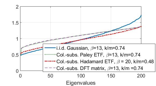
Figure 5: Sample spectrum of $S_{A}^{\top}S_{A}$ for various constructions with high redundancy, and small $k$ (normalized).

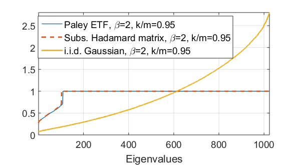
Figure 6: Sample spectrum of $S_{A}^{\top}S_{A}$ for various constructions with moderate redundancy, and large $k$ (normalized).

Although the derivation of tight eigenvalue bounds for subsampled ETFs is a long-standing problem, numerical evidence (see Figures 6, 6) suggests that they tend to have their eigenvalues more tightly concentrated around 1 than random matrices (also supported by the fact that they satisfy Welch bound, Proposition 7 with equality).

Note that our theoretical results focus on the extreme eigenvalues due to a worst-case analysis; in practice, most of the energy of the gradient lies on the eigen-space associated with the bulk of the eigenvalues, which the following proposition shows can be identically 1.

Proposition 8

If the rows of $S$ are chosen to form an ETF with redundancy $\beta$, then for $\eta\geq 1-\frac{1}{\beta}$, $\frac{1}{\beta}S_{A}^{\top}S_{A}$ has $n(1-\beta(1-\eta))$ eigenvalues equal to 1.

This follows immediately from Cauchy interlacing theorem, using the fact that $S_{A}S_{A}^{\top}$ and $S_{A}^{\top}S_{A}$ have the same spectra except zeros. Therefore for sufficiently large $\eta$, ETFs have a mostly flat spectrum even for low redundancy, and thus in practice one would expect ETFs to perform well even for small amounts of redundancy. This is also confirmed by Figure 6, as well as our numerical results.

Random matrices.

Another natural choice of encoding could be to use i.i.d. random matrices. Although encoding with such random matrices can be computationally expensive and may not have the desirable properties of encoding with tight frames, their eigenvalue behavior can be characterized analytically. In particular, using the existing results on the eigenvalue scaling of large i.i.d. Gaussian matrices from Geman (1980); Silverstein (1985) and union bound, it can be shown that

$$\mathbb{P}\left(\max_{A:\left|A\right|=k}\lambda_{\max}\left(\frac{1}{\beta\eta n}S_{A}^{\top}S_{A}\right)>\left(1+\sqrt{\frac{1}{\beta\eta}}\right)^{2}\right)\to 0$$ (8)

$$\mathbb{P}\left(\min_{A:\left|A\right|=k}\lambda_{\min}\left(\frac{1}{\beta\eta n}S_{A}^{\top}S_{A}\right)<\left(1-\sqrt{\frac{1}{\beta\eta}}\right)^{2}\right)\to 0,$$ (9)

as $n\to\infty$, if the elements of $S_{A}$ are drawn i.i.d. from $N(0,1)$. Hence, for sufficiently large redundancy and problem dimension, i.i.d. random matrices are good candidates for encoding as well. However, for finite $\beta$, even if $k=m$, in general the optimum of the original problem is not recovered exactly, for such matrices.

4.2 Efficient encoding

In this section we discuss some of the possible practical approaches to encoding. Some of the practical issues involving encoding include the the computational complexity of encoding, as well as the loss of sparsity in the data due to the multiplication with $S$, and the resulting increase in time and space complexity. We address these issues in this section.

4.2.1 Efficient distributed encoding with sparse matrices

Let the dataset $(X,y)$ lie in a database, accessible to each worker node, where each node is responsible for computing their own encoded partitions $S_{i}X$ and $S_{i}y$. We assume that $S$ has a sparse structure. Given $S$, define $B_{i}(S)=\left\{j:S_{ij}\neq 0\right\}$ as the set of indices of the non-zero elements of the $i$th row of $S$. For a set $\mathcal{I}$ of rows, we define $B_{\mathcal{I}}(S)=\cup_{i\in\mathcal{I}}B_{i}(S)$.

Let us partition the set of rows of $S$, $[\beta n]$, into $m$ machines, and denote the partition of machine $k$ as $\mathcal{I}_{k}$, i.e., $\bigsqcup_{k=1}^{m}\mathcal{I}_{k}=[\beta n]$, where $\sqcup$ denotes disjoint union. Then the set of non-zero columns of $S_{k}$ is given by $B_{\mathcal{I}_{k}}(S)$. Note that in order to compute $S_{k}X$, machine $k$ only requires the rows of $X$ in the set $B_{\mathcal{I}_{k}}(S)$. In what follows, we will denote this submatrix of $X$ by $\widetilde{X}_{k}$, i.e., if $x_{i}^{\top}$ is the $i$th row of $X$, $\widetilde{X}_{k}:=\left[x_{i}^{\top}\right]_{i\in B_{\mathcal{I}_{k}}(S)}$. Similarly $\widetilde{y}_{k}=\left[y_{i}\right]_{i\in B_{\mathcal{I}_{k}}(S)}$, where $y_{i}$ is the $i$th element of $y$.

Consider the specific computation that needs to be done by worker $k$ during the iterations, for each algorithm. Under the data parallelism setting, worker $k$ computes the following gradient:

$$\nabla f_{k}(w)=X^{\top}S_{k}^{\top}S_{k}(Xw-y)\overset{\mathrm{(a)}}{=}\widetilde{X}_{k}^{\top}S_{k}^{\top}S_{k}(\widetilde{X}_{k}w-\widetilde{y}_{k})$$ (10)

where (a) follows since the rows of $X$ that are not in $B_{\mathcal{I}_{k}}$ get multiplied by zero vector. Note that the last expression can be computed without any matrix-matrix multiplication. This gives a natural storage and computation scheme for the workers. Instead of computing $S_{k}X$ offline and storing it, which can result in a loss of sparsity in the data, worker $k$ can store $\widetilde{X}_{k}$ in uncoded form, and compute the gradient through (10) whenever needed, using only matrix-vector multiplications. Since $S_{k}$ is sparse, the overhead associated with multiplications of the form $S_{k}v$ and $S_{k}^{\top}v$ is small.

Similarly, under model parallelism, the computation required by worker $k$ is

$$\nabla_{k}\widetilde{g}(v)=S_{k}X^{\top}\nabla_{k}\phi\left(XS^{\top}_{k}v_{k}+\widetilde{z}_{k}\right)=S_{k}\widetilde{X}_{k}^{\top}\nabla_{k}\phi\left(\widetilde{X}_{k}S^{\top}_{k}v_{k}+\widetilde{z}_{k}\right),$$ (11)

and as in the data parallelism case, the worker can store $\widetilde{X}_{k}$ uncoded, and compute (11) online through matrix-vector multiplications.

Example: Steiner ETF.

We illustrate the described technique through Steiner ETF, based on the construction proposed in Fickus et al. (2012), using $(2,2,v)$-Steiner systems. Let $v$ be a power of 2, let $H\in\mathbb{R}^{v\times v}$ be a real Hadamard matrix, and let $h_{i}$ be the $i$th column of $H$, for $i=1,\dots,v$. Consider the matrix $V\in\left\{0,1\right\}^{v\times v(v-1)/2}$, where each column is the incidence vector of a distinct two-element subset of $\left\{1,\dots,v\right\}$. For instance, for $v=4$,

$$V=\left[\begin{array}[]{cccccc}1&1&1&0&0&0\\ 1&0&0&1&1&0\\ 0&1&0&1&0&1\\ 0&0&1&0&1&1\end{array}\right].$$

Note that each of the $v$ rows have exactly $v-1$ non-zero elements. We construct Steiner ETF $S$ as a $v^{2}\times\frac{v(v-1)}{2}$ matrix by replacing each 1 in a row with a distinct column of $H$, and normalizing by $\sqrt{v-1}$. For instance, for the above example, we have

$$S=\frac{1}{\sqrt{3}}\left[\begin{array}[]{cccccc}h_{2}&h_{3}&h_{4}&0&0&0\\ h_{2}&0&0&h_{3}&h_{4}&0\\ 0&h_{2}&0&h_{3}&0&h_{4}\\ 0&0&h_{2}&0&h_{3}&h_{4}\end{array}\right].$$

We will call a set of rows of $S$ that arises from the same row of $V$ a block. In general, this procedure results in a matrix $S$ with redundancy factor $\beta=\frac{2v}{v-1}$. In full generality, Steiner ETFs can be constructed for larger redundancy levels; we refer the reader to Fickus et al. (2012) for a full discussion of these constructions.

We partition the rows of the $V$ matrix into $m$ machines, so that each machine gets assigned $\frac{v}{m}$ rows of $V$, and thus the corresponding $\frac{v}{m}$ blocks of $S$.

This construction and partitioning scheme is particularly attractive for our purposes for two reasons. First, it is easy to see that for any node $k$, $\left|B_{\mathcal{I}_{k}}\right|$ is upper bounded by $\frac{v(v-1)}{m}=\frac{2n}{m}$, which means the memory overhead compared to the uncoded case is limited to a factor of $\beta$. Second, each block of $S_{k}$ consists of (almost) a Hadamard matrix, so the multiplication $S_{k}v$ can be efficiently implemented through Fast Walsh-Hadamard Transform.

Example: Haar matrix.

Another possible choice of sparse matrix is column-subsampled Haar matrix, which is defined recursively by

$$H_{2n}=\frac{1}{\sqrt{2}}\left[\begin{array}[]{c}H_{n}\otimes\left[1\;1\right]\\ I_{n}\otimes\left[1\;-1\right]\end{array}\right],\;\;H_{1}=1,$$

where $\otimes$ denotes Kronecker product. Given a redundancy level $\beta$, one can obtain $S$ by randomly sampling $\frac{n}{\beta}$ columns of $H_{n}$. It can be shown that in this case, we have $\left|B_{\mathcal{I}_{k}}\right|\leq\frac{\beta n\log(n)}{m}$, and hence encoding with Haar matrix incurs a memory cost by logarithmic factor.

4.2.2 Fast transforms

Another computationally efficient method for encoding is to use fast transforms: Fast Fourier Transform (FFT), if $S$ is chosen as a subsampled DFT matrix, and the Fast Walsh-Hadamard Transform (FWHT), if $S$ is chosen as a subsampled real Hadamard matrix. In particular, one can insert rows of zeroes at random locations into the data pair $(X,y)$, and then take the FFT or FWHT of each column of the augmented matrix. This is equivalent to a randomized Fourier or Hadamard ensemble, which is known to satisfy the RIP with high probability by Candes and Tao (2006). However, such transforms do not have the memory advantages of the sparse matrices, and thus they are more useful for the setting where the dataset is dense, and the encoding is done offline.

4.3 Cost of encoding

Since encoding increases the problem dimensions, it clearly comes with the cost of increased space complexity. The memory and storage requirement of the optimization still increases by a factor of 2, if the encoding is done offline (for dense datasets), or if the techniques described in the previous subsection are applied (for sparse datasets). Note that the added redundancy can come by increasing the amount of effective data points per machine, by increasing the number of machines while keeping the load per machine constant, or a combination of the two. In the first case, the computational load per machine increases by a factor of $\beta$. Although this can make a difference if the system is bottlenecked by the computation time, distributed computing systems are typically communication-limited, and thus we do not expect this additional cost to dominate the speed-up from the mitigation of stragglers.

5 Numerical Results

We implement the proposed technique on four problems: ridge regression, matrix factorization, logistic regression, and LASSO.

5.1 Ridge regression

We generate the elements of matrix $X$ i.i.d. $\sim N(0,1)$, and the elements of $y$ are generated from $X$ and an i.i.d. $N(0,1)$ parameter vector $w^{*}$, through a linear model with Gaussian noise, for dimensions $(n,p)=(4096,6000)$. We solve the problem $\min_{w}\frac{1}{2n}\left\|S\left(Xw-y\right)\right\|^{2}+\frac{\lambda}{2}\|w\|^{2}$, for regularization parameter $\lambda=0.05$. We evaluate column-subsampled Hadamard matrix with redundancy $\beta=2$ (encoded using FWHT), replication and uncoded schemes. We implement distributed L-BFGS as described in Section 3 on an Amazon EC2 cluster using mpi4py Python package, over $m=32$ m1.small instances as worker nodes, and a single c3.8xlarge instance as the central server.

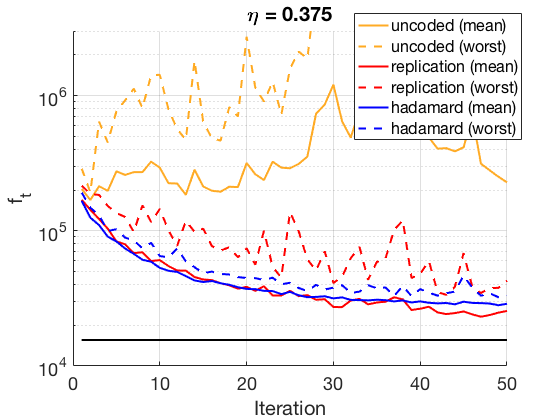
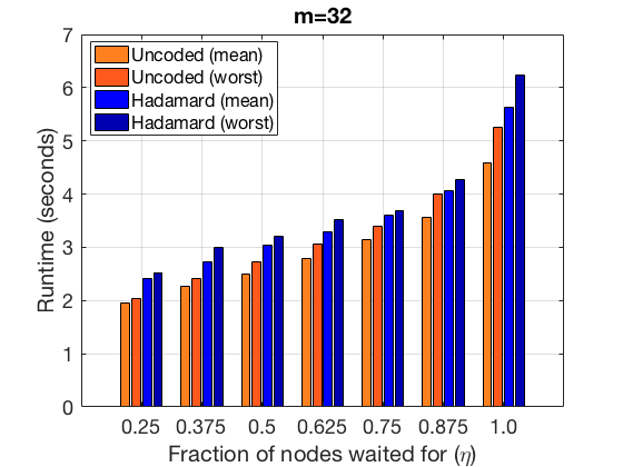
Figure 7: Left: Sample evolution of uncoded, replication, and Hadamard (FWHT)-coded cases, for $k=12$, $m=32$. Right: Runtimes of the schemes for different values of $\eta$, for the same number of iterations for each scheme. Note that this essentially captures the delay profile of the network, and does not reflect the relative convergence rates of different methods.

Figure 7 shows the result of our experiments, which are aggregated from 20 trials. In addition to uncoded scheme, we consider data replication, where each uncoded partition is replicated $\beta=2$ times across nodes, and the server discards the duplicate copies of a partition, if received in an iteration. It can be seen that for low $\eta$, uncoded L-BFGS may not converge when a fixed number of nodes are waited for, whereas the Hadamard-coded case stably converges. We also observe that the data replication scheme converges on average, but its performance may deteriorate if both copies of a partition are delayed. Figure 7 suggests that this performance can be achieved with an approximately $40\%$ reduction in the runtime, compared to waiting for all the nodes.

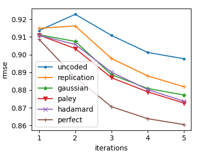
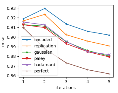
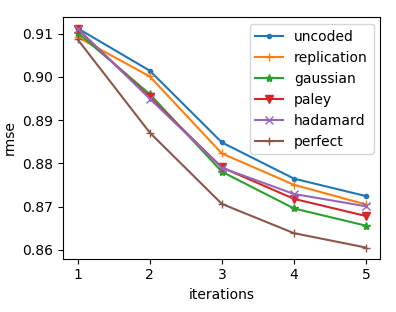
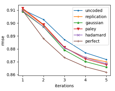
Figure 8: Test RMSE for $m=8$ (left) and $m=24$ (right) nodes, where the server waits for $k=m/8$ (top) and $k=m/2$ (bottom) responses. “Perfect” refers to the case where $k=m$.

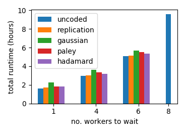
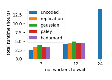
Figure 9: Total runtime with $m=8$ and $m=24$ nodes for different values of $k$, under fixed 100 iterations for each scheme.

5.2 Matrix factorization

We next apply matrix factorization on the MovieLens-1M dataset (Riedl and Konstan (1998)) for the movie recommendation task. We are given $R$, a sparse matrix of movie ratings 1–5, of dimension $\#users\times\#movies$, where $R_{ij}$ is specified if user $i$ has rated movie $j$. We withhold randomly 20% of these ratings to form an 80/20 train/test split. The goal is to recover user vectors $x_{i}\in\mathbb{R}^{p}$ and movie vectors $y_{i}\in\mathbb{R}^{p}$ (where $p$ is the embedding dimension) such that $R_{ij}\approx x_{i}^{T}y_{j}+u_{i}+v_{j}+b$, where $u_{i}$, $v_{j}$, and $b$ are user, movie, and global biases, respectively. The optimization problem is given by

$$\min_{x_{i},y_{j},u_{i},v_{j}}\sum_{i,j\text{: observed}}(R_{ij}-u_{i}-v_{j}-x_{i}^{T}y_{j}-b)^{2}+\lambda\left(\sum_{i}\|x_{i}\|_{2}^{2}+\|u\|_{2}^{2}+\sum_{j}\|y_{j}\|_{2}^{2}+\|v\|_{2}^{2}\right).$$ (12)

We choose $b=3$, $p=15$, and $\lambda=10$, which achieves test RMSE 0.861, close to the current best test RMSE on this dataset using matrix factorization.

Problem (12) is often solved using alternating minimization, minimizing first over all $\left(x_{i},u_{i}\right)$, and then all $\left(y_{j},v_{j}\right)$, in repetition. Each such step further decomposes by row and column, made smaller by the sparsity of $R$. To solve for $\left(x_{i},u_{i}\right)$, we first extract $I_{i}=\{j\mid r_{ij}\text{ is observed}\}$, and minimize

$$\left(\left[\begin{matrix}y_{I_{i}}^{T},\mathbf{1}\end{matrix}\right]\left[\begin{matrix}x_{i}\\ u_{i}\end{matrix}\right]-(R_{i,I_{i}}^{T}-v_{I_{i}}-b\mathbf{1})\right)^{2}+\lambda\left(\sum_{i}\|x_{i}\|_{2}^{2}+\|u\|_{2}^{2}\right)$$ (13)

for each $i$, which gives a sequence of regularized least squares problems with variable $w=[x_{i}^{T},u_{i}]^{T}$, which we solve distributedly using coded L-BFGS; and repeat for $w=[y_{j}^{T},v_{j}]^{T}$, for all $j$.

The Movielens experiment is run on a single 32-core machine with Linux 4.4. In order to simulate network latency, an artificial delay of $\Delta\sim\text{exp}(\text{10 ms})$ is imposed each time the worker completes a task. Small problem instances ($n<500$) are solved locally at the central server, using the built-in function numpy.linalg.solve. To reduce overhead, we create a bank of encoding matrices $\left\{S_{n}\right\}$ for Paley ETF and Hadamard ETF, for $n=100,200,\ldots,3500$, and then given a problem instance, subsample the columns of the appropriate matrix $S_{n}$ to match the dimensions. Overall, we observe that encoding overhead is amortized by the speed-up of the distributed optimization.

Figure 9 gives the final performance of our distributed L-BFGS for various encoding schemes, for each of the 5 epochs, which shows that coded schemes are most robust for small $k$. A full table of results is given in Appendix D.

5.3 Logistic regression

In our next experiment, we apply logistic regression for document classification for Reuters Corpus Volume 1 (rcv1.binary) dataset from Lewis et al. (2004), where we consider the binary task of classifying the documents into corporate/industrial/economics vs. government/social/markets topics. The dataset has 697,641 documents, and 47,250 term frequency-inverse document frequency (tf-idf) features. We randomly select 32,500 features for the experiment, and reserve 100,000 documents for the test set. We use logistic regression with $\ell_{2}$-regularization for the classification task, with the objective

$$\min_{w,b}\frac{1}{n}\sum_{i=1}^{n}\log\left(1+\exp\left\{-z_{i}^{\top}w+b\right\}\right)+\lambda\|w\|^{2},$$

where $z_{i}=y_{i}x_{i}$ is the data sample $x_{i}$ multiplied by the label $y_{i}\in\left\{-1,1\right\}$, and $b$ is the bias variable. We solve this optimization using encoded distributed block coordinate descent as described in Section 2, and implement Steiner and Haar encoding as described in Section 4, with redundancy $\beta=2$. In addition we implement the asynchronous coordinate descent, as well as replication, which represents the case where each partition $Z_{i}$ is replicated across two nodes, and the faster copy is used in each iteration. We use $m=128$ t2.medium instances as worker nodes, and a single c3.4xlarge instance as the master node, which communicate using the mpi4py package. We consider two models for stragglers. In the first model, at each node, we add a random delay drawn from a Gaussian mixture distribution $q\mathcal{N}(\mu_{1},\sigma_{1}^{2})+(1-q)\mathcal{N}(\mu_{2},\sigma_{2}^{2})$, where $q=0.5$, $\mu_{1}=0.5$s, $\mu_{2}=20$s, $\sigma_{1}=0.2$s, $\sigma_{2}=5$s. In the second model, we do not directly add any delay, but at each machine we launch a number of dummy background tasks (matrix multiplication) that are executed throughout the computation. The number of background tasks across the nodes is distributed according to a power law with exponent $\alpha=1.5$. The number of background tasks launched is capped at 50.

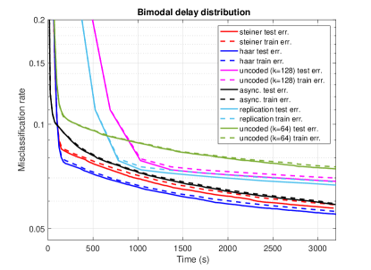
Figure 10: Test and train errors over time (in seconds) for each scheme, for the bimodal delay distribution. Steiner and Haar encoding is done with $k=64$, $\beta=2$.

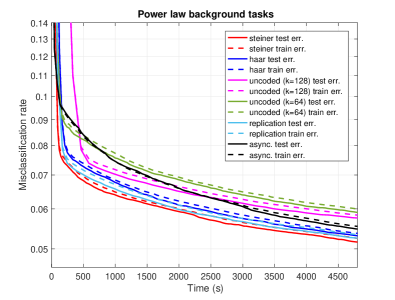
Figure 11: Test and train errors over time (in seconds) for each scheme. Number of background tasks follow a power law. Steiner and Haar encoding is done with $k=80$, $\beta=2$.

Figure 12: The fraction of iterations each worker node participates in (the empirical probability of the event $\{k\in A_{t}\}$), plotted for Steiner encoding with $k=80$, $m=128$. The number of background tasks are distributed by a power law with $\alpha=1.5$ (capped at 50).

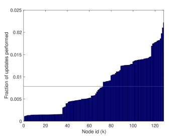
Figure 13: The fraction of updates performed by each node, for asynchronous block coordinate descent. The horizontal line represents the uniformly distributed case. The number of background tasks are distributed by a power law with $\alpha=1.5$ (capped at 50).

Figures 11 and 11 shows the evolution of training and test errors as a function of wall clock time. We observe that for each straggler model, either Steiner or Haar encoded optimization dominates all schemes. Figures 13 and 13 show the statistics of how frequent each node participates in an update, for the case with background tasks, for encoded and asynchronous cases, respectively. We observe that the stark difference in the relative speeds of different machines result in vastly different update frequencies for the asynchronous case, which results in updates with large delays, and a corresponding performance loss.

5.4 LASSO

We solve the LASSO problem, with the objective

$$\min_{w}\frac{1}{2n}\|Xw-y\|^{2}+\lambda\|w\|_{1}^{2},$$

where $X\in\mathbb{R}^{130,000\times 100,000}$ is a matrix with i.i.d. $N(0,1)$ entries, and $y$ is generated from $X$ and a parameter vector $w^{*}$ through a linear model with Gaussian noise:

$$y=Xw^{*}+\sigma z,$$

where $\sigma=40$, $z\sim N(0,1)$. The parameter vector $w^{*}$ has 7695 non-zero entries out of 100,000, where the non-zero entries are generated i.i.d. from $N(0,4)$. We choose $\lambda=0.6$ and consider the sparsity recovery performance of the corresponding LASSO problem, solved using proximal gradient (iterative shrinkage/thresholding algorithm).

We implement the algorithm over 128 t2.medium worker nodes which collectively store the matrix $X$, and a c3.4xlarge master node. We measure the sparsity recovery performance of the solution using the F1 score, defined as the harmonic mean

$$F1=\frac{2PR}{P+R},$$

where $P$ and $R$ are precision recall of the solution vector $\hat{w}$ respectively, defined as

$$P=\frac{\left|\left\{i:w^{*}_{i}\neq 0,\hat{w}_{i}\neq 0\right\}\right|}{\left|i:\hat{w}_{i}\neq 0\right|},\;\;R=\frac{\left|\left\{i:w^{*}_{i}\neq 0,\hat{w}_{i}\neq 0\right\}\right|}{\left|i:w^{*}_{i}\neq 0\right|}$$

.

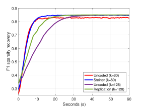
Figure 14: Evolution of F1 sparsity recovery performance for each scheme.

Figure 14 shows the sample evolution of the F1 score of the model under uncoded, replication, and Steiner encoded scenarios, with artificial multi-modal communication delay distribution $q_{1}\mathcal{N}(\mu_{1},\sigma_{1}^{2})+q_{2}\mathcal{N}(\mu_{2},\sigma_{2}^{2})+q_{3}\mathcal{N}(\mu_{3},\sigma_{3}^{2})$, where $q_{1}=0.8$, $q_{2}=0.1$, $q_{3}=0.1$; $\mu_{1}=0.2$s, $\mu_{2}=0.6$s, $\mu_{3}=1$s; and $\sigma_{1}=0.1$s, $\sigma=0.2$s, $\sigma_{3}=0.4$s, independently at each node. We observe that the uncoded case $k=80$ results in a performance loss in sparsity recovery due to data dropped from delayed noes, and uncoded and replication with $k=128$ converges slow due to stragglers, while Steiner coding with $k=80$ is not delayed by stragglers, while maintaining almost the same sparsity recovery performance as the solution of the uncoded $k=128$ case.

Acknowledgments

The work of Can Karakus and Suhas Diggavi was supported in part by NSF grants #1314937 and #1514531. The work of Wotao Yin was supported by ONR Grant N000141712162, and NSF Grant DMS-1720237.

A Proofs of Theorems 2 and 4

In the proofs, we will ignore the normalization constants on the objective functions for brevity. We will assume the normalization $\frac{1}{\sqrt{\eta}}$ is absorbed into the encoding matrix $S_{A}$. Let $\widetilde{f}^{A}_{t}:=\|S_{A_{t}}\left(Xw_{t}-y\right)\|^{2}+\lambda h(w)$, and $\widetilde{f}^{A}(w):=\|S_{A_{t}}\left(Xw-y\right)\|^{2}+\lambda h(w)$, where we set $A\equiv A_{t}$. Let $\widetilde{w}_{t}^{*}$ denote the solution to the effective “instantaneous” problem at iteration $t$, i.e., $\widetilde{w}_{t}^{*}=\operatorname*{arg\,min}_{w}\widetilde{f}^{A}(w)$.

Throughout this appendix, we will also denote

$$w^{*} =\operatorname*{arg\,min}_{w}\|Xw-y\|^{2}+\lambda h(w)$$

$$\hat{w} =\operatorname*{arg\,min}_{w}\|S_{A}\left(Xw-y\right)\|^{2}+\lambda h(w)$$

unless otherwise noted, where $A$ is a fixed subset of $[m]$.

A.1 Lemmas

Lemma 9

If $S$ satisfies (6) for any $A\subseteq[m]$ with $\left|A\right|\geq k$, for any convex set $C$,

$$\|X\hat{w}-y\|^{2}\leq\kappa^{2}\|Xw^{*}-y\|^{2},$$

where $\kappa=\frac{1+\epsilon}{1-\epsilon}$, $\hat{w}=\operatorname*{arg\,min}_{w\in C}\|S_{A}\left(Xw-y\right)\|^{2}$, and $w^{*}=\operatorname*{arg\,min}_{w\in C}\|Xw-y\|^{2}$.

Proof  Define $e=\hat{w}-w^{*}$ and note that

$$\|X\hat{w}-y\|=\|Xw^{*}-y+Xe\|\leq\|Xw^{*}-y\|+\|Xe\|$$

by triangle inequality, which implies

$$\|X\hat{w}-y\|^{2}\leq\left(1+\frac{\|Xe\|}{\|Xw^{*}-y\|}\right)^{2}\|Xw^{*}-y\|^{2}=\left(1+\frac{\|Xe\|}{\|Xw^{*}-y\|}\right)^{2}\|Xw^{*}-y\|^{2}.$$ (14)

Now, for any $c>0$, consider

$$\|Xe\|^{2} \leq\frac{\|S_{A}Xe\|^{2}}{1-\epsilon}\overset{\mathrm{(a)}}{\leq}-2\frac{e^{\top}X^{\top}S_{A}^{\top}S_{A}(Xw^{*}-y)}{1-\epsilon}$$

$$=-2\frac{e^{\top}X^{\top}\left(S_{A}^{\top}S_{A}-cI\right)(Xw^{*}-y)}{1-\epsilon}-\frac{2c}{1-\epsilon}e^{\top}X^{\top}(Xw^{*}-y)$$

$$\overset{\mathrm{(b)}}{\leq}-2\frac{e^{\top}X^{\top}\left(S_{A}^{\top}S_{A}-cI\right)(Xw^{*}-y)}{1-\epsilon}$$

$$\overset{\mathrm{(c)}}{\leq}2\frac{\left\|e^{\top}X^{\top}\left(cI-S_{A}^{\top}S_{A}\right)\right\|}{1-\epsilon}\|Xw^{*}-y\|$$

$$\overset{\mathrm{(d)}}{\leq}2\frac{\left\|cI-S_{A}^{\top}S_{A}\right\|}{1-\epsilon}\|Xw^{*}-y\|\|Xe\|,$$

where (a) follows by expanding and re-arranging $\left\|S_{A}\left(X\hat{w}-y\right)\right\|^{2}\leq\left\|S_{A}\left(Xw^{*}-y\right)\right\|^{2}$, which is true since $\hat{w}$ is the minimizer of this function; (b) follows by the fact that since $\hat{w}\in C$, $e$ represents a feasible direction of the constrained optimization, and thus the convex optimality condition implies $\langle\nabla f(w^{*}),\hat{w}-w^{*}\rangle=e^{\top}X^{\top}(Xw^{*}-y)\geq 0$; (c) follows by Cauchy-Schwarz inequality; and (d) follows by the definition of matrix norm.

Since this is true for any $c>0$, we make the minimizing choice $c=\frac{\lambda_{\max}+\lambda_{\min}}{2}$ (where $\lambda_{\max}$ and $\lambda_{\min}$ represent the largest and smallest eigenvalues of $S_{A}^{\top}S_{A}$, respectively), which gives

$$\frac{\|Xe\|}{\|X\hat{w}-y\|}\leq\frac{\lambda_{\max}-\lambda_{\min}}{\lambda_{\min}}\leq\frac{2\epsilon}{1-\epsilon}.$$

Plugging this back in (14), we get the desired result.  

Lemma 10

If $S$ satisfies (6) for any $A\subseteq[m]$ with $\left|A\right|\geq k$,

$$f(\hat{w})\leq\kappa^{2}f(w^{*}),$$

where $\kappa=\frac{1+\epsilon}{1-\epsilon}$, $\hat{w}=\operatorname*{arg\,min}_{w}\|S_{A}\left(Xw-y\right)\|^{2}+\lambda h(w)$, and $w^{*}=\operatorname*{arg\,min}_{w}\|Xw-y\|^{2}+\lambda h(w)$.

Proof  Consider a fixed $A_{t}=A$, and a corresponding

$$\hat{w}=\widetilde{w}_{t}^{*}\in\operatorname*{arg\,min}_{w}\|S_{A}\left(Xw-y\right)\|^{2}+\lambda h(w)$$

Define

$$\hat{w}(r) =\operatorname*{arg\,min}_{w:\lambda h(w)\leq r}\|S_{A}\left(Xw-y\right)\|^{2}$$

$$w^{*}(r) =\operatorname*{arg\,min}_{w:\lambda h(w)\leq r}\|Xw-y\|^{2}.$$

Finally, define

$$r^{*}=\operatorname*{arg\,min}_{r}\|Xw^{*}(r)-y\|^{2}+r.$$

Now, consider

$$f(\hat{w}) =\|X\hat{w}-y\|^{2}+\lambda h(w)=\min_{r}\left(\|X\hat{w}(r)-y\|^{2}+r\right)$$

$$\leq\|X\hat{w}(r^{*})-y\|^{2}+r^{*}\overset{\mathrm{(a)}}{\leq}\kappa^{2}\|Xw^{*}(r^{*})-y\|^{2}+r^{*}$$

$$\leq\kappa^{2}\left(\|Xw^{*}(r^{*})-y\|^{2}+r^{*}\right)=\kappa^{2}f(w^{*}),$$

which shows the desired result, where (a) follows by Lemma 9, and by the fact that the set $\left\{w:\lambda h(w)\leq r\right\}$ is a convex set.  

Lemma 11

If

$$\widetilde{f}^{A}_{t+1}-\widetilde{f}^{A}\left(\widetilde{w}^{*}_{t}\right)\leq\gamma\left(\widetilde{f}^{A}_{t}-\widetilde{f}^{A}\left(\widetilde{w}^{*}_{t}\right)\right)$$

for all $t>0$, and for some $0<\gamma<1$, where $\widetilde{w}^{*}_{t}\in\operatorname*{arg\,min}_{w}\widetilde{f}_{t}^{A}$, then

$$f(w_{t})\leq\left(\kappa\gamma\right)^{t}f(w_{0})+\frac{\kappa^{2}\left(\kappa-\gamma\right)}{1-\kappa\gamma}f\left(w^{*}\right),$$

where $\kappa=\frac{1+\epsilon}{1-\epsilon}$.

Proof  Since for any $w$,

$$\left(1-\epsilon\right)\|Xw-y\|^{2}\leq\left(Xw-y\right)^{\top}S_{A}^{\top}\widetilde{S}_{A}\left(Xw-y\right),$$

we have

$$\left(1-\epsilon\right)f(w)\leq\widetilde{f}^{A}(w).$$

Similarly $\widetilde{f}^{A}(w)\leq\left(1+\epsilon\right)f(w)$, and therefore, using the assumption of the theorem

$$\left(1-\epsilon\right)f(w_{t+1})-\left(1+\epsilon\right)f\left(\widetilde{w}_{t}^{*}\right)\leq\gamma\left(\left(1+\epsilon\right)f(w_{t})-\left(1-\epsilon\right)f\left(\widetilde{w}_{t}^{*}\right)\right),$$

which can be re-arranged into the linear recursive inequality

$$f(w_{t+1})\leq\kappa\gamma f_{t}+(\kappa-\gamma)f\left(\widetilde{w}_{t}^{*}\right)\overset{\mathrm{(a)}}{\leq}\kappa\gamma f(w_{t})+\kappa^{2}(\kappa-\gamma)f\left(w^{*}\right),$$

where $\kappa=\frac{1+\epsilon}{1-\epsilon}$ and (a) follows by Lemma 10. By considering such inequalities for $0\leq\tau\leq t$, multiplying each by $\left(\kappa\gamma\right)^{t-\tau}$ and summing, we get

$$f(w_{t}) \leq\left(\kappa\gamma\right)^{t}f(w_{0})+\kappa^{2}(\kappa-\gamma)f\left(w^{*}\right)\sum_{\tau=0}^{t-1}\left(\kappa\gamma\right)^{\tau}$$

$$\leq\left(\kappa\gamma\right)^{t}f(w_{0})+\frac{\kappa^{2}\left(\kappa-\gamma\right)}{1-\kappa\gamma}f\left(w^{*}\right).$$

 

Lemma 12

Under the assumptions of Theorem 4, $\widetilde{f}^{A}(w)$ is $\left(1-\epsilon\right)(\mu+\lambda)$-strongly convex.

Proof  It is sufficient to show that the minimum eigenvalue of $\widetilde{X}_{A}^{\top}\widetilde{X}_{A}$ is bounded away from zero. This can easily be shown by the fact that

$$u^{\top}\widetilde{X}_{A}^{\top}\widetilde{X}_{A}u=u^{\top}X^{\top}S_{A}^{\top}S_{A}Xu\geq\left(1-\epsilon\right)\|Xu\|^{2}\geq\left(1-\epsilon\right)\mu\|u\|^{2},$$

for any unit vector $u$.  

Lemma 13

Let $M\in\mathbb{R}^{p\times p}$ be a symmetric positive definite matrix, with the condition number (ratio of maximum eigenvalue to the minimum eigenvalue) given by $\kappa$. Then, for any unit vector $u$,

$$\frac{u^{\top}Mu}{\|Mu\|}\geq\frac{2\sqrt{\kappa}}{\kappa+1}.$$

Proof  We point out that this is a special case of Kantorovich inequality, but provide a dedicated proof here for completeness.

Let $M$ have the eigen-decomposition $M=Q^{\top}DQ$, where $Q$ has orthonormal columns, and $D$ is a diagonal matrix with positive, decreasing entries $d_{1}\geq d_{2}\geq\dots\geq d_{n}$, with $\frac{d_{1}}{d_{n}}=\kappa$. Let $y=\left(Qu\right)^{\circ 2}$, where ^∘2 denotes entry-wise square. Then the quantity we are interested in can be represented as

$$\frac{\sum_{i=1}^{n}d_{i}y_{i}}{\sqrt{\sum_{i=1}^{n}d_{i}^{2}y_{i}}},$$

which we would like to minimize subject to a simplex constraint $\mathbf{1}^{\top}y=1$. Using Lagrange multipliers, it can be seen that the minimum is attained where $y_{1}=\frac{1}{1+\kappa}$, $y_{n}=\frac{\kappa}{1+\kappa}$, and $y_{i}=0$ for $i\neq 1,n$. Plugging this back the objective, we get the desired result

$$\frac{u^{\top}Mu}{\|Mu\|}\geq\frac{2\sqrt{\kappa}}{\kappa+1}.$$

 

Proof  [Proof of Lemma 1] Define $\breve{S}_{t}:=S_{A_{t}\cap A_{t-1}}$. First note that

$$r_{t}^{\top}u_{t} =\left(X^{\top}\breve{S}_{t}^{\top}\breve{S}_{t}\left[(Xw_{t}-y)-(Xw_{t-1}-y)\right]\right)^{\top}\left(w_{t}-w_{t-1}\right)$$

$$=\left(w_{t}-w_{t-1}\right)^{\top}X^{\top}\breve{S}_{t}^{\top}\breve{S}_{t}X\left(w-w_{t-1}\right)$$

$$\geq\delta\mu\|u_{t}\|^{2},$$ (15)

by (5) Also consider

$$\frac{\|r_{t}\|^{2}}{r_{t}^{\top}u_{t}}=\frac{\left(w_{t}-w_{t-1}\right)^{\top}\left(X^{\top}\breve{S}_{t}^{\top}\breve{S}_{t}X\right)^{2}\left(w_{t}-w_{t-1}\right)}{\left(w_{t}-w_{t-1}\right)^{\top}X^{\top}\breve{S}_{t}^{\top}\breve{S}_{t}X\left(w_{t}-w_{t-1}\right)},$$

which implies

$$\epsilon\mu\leq\frac{\|r_{t}\|^{2}}{r_{t}^{\top}u_{t}}\leq(1+\epsilon)M,$$

again by (4). Now, setting $j_{\ell}=t-\widetilde{\sigma}+\ell$, consider the trace

$$\textbf{tr}\left(B_{t}^{(\ell+1)}\right) =\textbf{tr}\left(B_{t}^{(\ell)}\right)-\textbf{tr}\left(\frac{B_{t}^{(\ell)}u_{j_{\ell}}u_{j_{\ell}}^{\top}B_{t}^{(\ell)}}{u_{j_{\ell}}^{\top}B_{t}^{(\ell)}u_{j_{\ell}}}\right)+\textbf{tr}\left(\frac{r_{j_{\ell}}r_{j_{\ell}}^{\top}}{r_{j_{\ell}}^{\top}u_{j_{\ell}}}\right)$$

$$\leq\textbf{tr}\left(B_{t}^{(\ell)}\right)+\textbf{tr}\left(\frac{r_{j_{\ell}}r_{j_{\ell}}^{\top}}{r_{j_{\ell}}^{\top}u_{j_{\ell}}}\right)$$

$$=\textbf{tr}\left(B_{t}^{(\ell)}\right)+\frac{\|r_{j_{\ell}}\|^{2}}{r_{j_{\ell}}^{\top}u_{j_{\ell}}}$$

$$\leq\textbf{tr}\left(B_{t}^{(\ell)}\right)+(1+\epsilon)M,$$

which implies $\textbf{tr}\left(B_{t}\right)\leq(1+\epsilon)M\left(\widetilde{\sigma}+d\right)$. It can also be shown (similar to Berahas et al. (2016)) that

$$\det\left(B_{t}^{(\ell+1)}\right) =\det\left(B_{t}^{(\ell)}\right)\cdot\frac{r^{\top}_{j_{\ell}}u_{j_{\ell}}}{u_{j_{\ell}}^{\top}B_{t}^{(\ell)}u_{j_{\ell}}}$$

$$=\det\left(B_{t}^{(\ell)}\right)\cdot\frac{r^{\top}_{j_{\ell}}u_{j_{\ell}}}{\|u_{j_{\ell}}\|^{2}}\cdot\frac{\|u_{j_{\ell}}\|^{2}}{u_{j_{\ell}}^{\top}B_{t}^{(\ell)}u_{j_{\ell}}}$$

$$\geq\det\left(B_{t}^{(\ell)}\right)\frac{\delta\mu}{(1+\epsilon)M\left(\widetilde{\sigma}+d\right)},$$

which implies $\det\left(B_{t}\right)\geq\det\left(B_{t}^{(0)}\right)\left(\frac{\delta\mu}{(1+\epsilon)M\left(\widetilde{\sigma}+d\right)}\right)^{\widetilde{\sigma}}$. Since $B_{t}\geq 0$, its trace is bounded above, and its determinant is bounded away from zero, there must exist $0<c_{1}\leq c_{2}$ such that

$$c_{1}I\preceq B_{t}\preceq c_{2}I.$$

 

A.2 Proof of Theorem 2

The proof of the first part of the theorem is a special case of the proof of Theorem 5 (with $\lambda=0$, and the smooth regularizer incorporated into $p(w)$) and thus we omit this proof and refer the reader to Appendix B. We prove the second part here.

Note that because of the condition in (6), we have

$$(1-\epsilon)\preceq S_{A}^{\top}S_{A}\preceq(1+\epsilon)I,$$

$$(1-\epsilon)\preceq S_{D}^{\top}S_{D}\preceq(1+\epsilon)I.$$

Using smoothness of the objective, and the choices $d_{t}=-\nabla\widetilde{f}^{A}(w_{t})(w_{t})$ and $\alpha_{t}=\alpha$, we have

$$\widetilde{f}^{A}\left(w_{t+1}\right)-\widetilde{f}^{A}(w_{t})\leq\alpha\nabla\widetilde{f}^{A}(w_{t})(w_{t})^{\top}d_{t}+\frac{1}{2}\alpha^{2}d_{t}^{\top}X^{\top}S_{A}^{\top}S_{A}Xd_{t}+\frac{L}{2}\alpha^{2}\|d_{t}\|^{2}$$

$$\leq-\alpha\left(1-\frac{(1+\epsilon)M+L}{2}\alpha\right)\left\|\nabla\widetilde{f}^{A}(w_{t})\right\|^{2}=-\frac{2\zeta\left(1-\zeta\right)}{(1+\epsilon)M+L}\|\nabla\widetilde{f}^{A}(w_{t})\|^{2}$$

$$\overset{\mathrm{(a)}}{\leq}-\frac{4\nu\zeta\left(1-\zeta\right)}{M\left(1+\epsilon\right)+L}\left(\widetilde{f}^{A}\left(w_{t}\right)-\widetilde{f}^{A}\left(\widetilde{w}_{t}^{*}\right)\right),$$

where (a) follows by strong convexity. Re-arranging this inequality, and using the definition of $\gamma$, we get

$$\widetilde{f}^{A}_{t+1}-\widetilde{f}^{A}\left(\widetilde{w}_{t}^{*}\right)\leq\gamma\left(\widetilde{f}^{A}_{t}-\widetilde{f}^{A}\left(\widetilde{w}_{t}^{*}\right)\right),$$

which, using Lemma 11, implies the result.

A.3 Proof of Theorem 4

Since $h(w)$ is constrained to be quadratic, we can absorb this term into the error term to get

$$\min_{w}\left\|\left[\begin{array}[]{cc}S&0\\ 0&I\end{array}\right]\left(\left[\begin{array}[]{c}X\\ \sqrt{\lambda}I\end{array}\right]w-\left[\begin{array}[]{c}y\\ 0\end{array}\right]\right)\right\|.$$

Note that as long as $S$ satisfies (6), the effective encoding matrix $\text{diag}\left(\left[S,I\right]\right)$ also satisfies the same. Therefore, without loss of generality we can ignore $h(w)$, and assume

$$(\mu+\lambda)I\preceq X^{\top}X\preceq(M+\lambda)I.$$

We also define $\lambda_{\min}=1-\epsilon$ and $\lambda_{\max}=1+\epsilon$ for convenience. Using convexity and the closed-form expression for the step size, we have

$$\widetilde{f}^{A}\left(w_{t+1}\right)-\widetilde{f}^{A}(w_{t})\leq\alpha_{t}\nabla\widetilde{f}^{A}(w_{t})^{\top}d_{t}+\frac{1}{2}\alpha_{t}^{2}d_{t}^{\top}X^{\top}S_{A}^{\top}S_{A}Xd_{t}$$

$$=-\frac{\rho\left(\nabla\widetilde{f}^{A}(w_{t})^{\top}d_{t}\right)^{2}}{d_{t}^{\top}X^{\top}S_{D}^{\top}S_{D}Xd_{t}}+\frac{1}{2}\frac{\rho^{2}\left(\nabla\widetilde{f}^{A}(w_{t})^{\top}d_{t}\right)^{2}}{d_{t}^{\top}X^{\top}S_{D}^{\top}S_{D}Xd_{t}}\cdot\frac{d_{t}^{\top}X^{\top}S_{A}^{\top}S_{A}Xd_{t}}{d_{t}^{\top}X^{\top}S_{D}^{\top}S_{D}Xd_{t}}$$

$$=\left(\frac{d_{t}^{\top}X^{\top}\left(\rho^{2}S_{A}^{\top}S_{A}-2\rho S_{D}^{\top}S_{D}\right)Xd_{t}}{2\left(d_{t}^{\top}X^{\top}S_{D}^{\top}S_{D}Xd_{t}\right)^{2}}\right)\left(d_{t}^{\top}\nabla\widetilde{f}^{A}(w_{t})\right)^{2}$$

$$\overset{\mathrm{(a)}}{=}-\rho\left(\frac{z^{\top}\left(S_{D}^{\top}S_{D}-\frac{\rho}{2}S_{A}^{\top}S_{A}\right)z}{\left(z^{\top}S_{D}^{\top}S_{D}z\right)^{2}}\right)\frac{\left(d_{t}^{\top}\nabla\widetilde{f}^{A}(w_{t})\right)^{2}}{\|Xd_{t}\|^{2}}$$

$$\overset{\mathrm{(b)}}{\leq}-\rho\left(\frac{\lambda_{\min}-\frac{\rho}{2}\lambda_{\max}}{\lambda_{\min}^{2}}\right)\frac{\left(d_{t}^{\top}\nabla\widetilde{f}^{A}(w_{t})\right)^{2}}{\|Xd_{t}\|^{2}}\overset{\mathrm{(c)}}{\leq}-\frac{\rho}{M+\lambda}\left(\frac{\lambda_{\min}-\frac{\rho}{2}\lambda_{\max}}{\lambda_{\min}^{2}}\right)\frac{\left(d_{t}^{\top}\nabla\widetilde{f}^{A}(w_{t})\right)^{2}}{\|d_{t}\|^{2}}$$

$$\overset{\mathrm{(d)}}{=}-\frac{\rho}{M+\lambda}\left(\frac{\lambda_{\min}-\frac{\rho}{2}\lambda_{\max}}{\lambda_{\min}^{2}}\right)\frac{\left(\nabla\widetilde{f}^{A}(w_{t})^{\top}B_{t}\nabla\widetilde{f}^{A}(w_{t})\right)^{2}}{\|B_{t}\nabla\widetilde{f}^{A}(w_{t})\|^{2}}$$

$$\overset{\mathrm{(e)}}{\leq}-\frac{4\rho}{M+\lambda}\left(\frac{\lambda_{\min}-\frac{\rho}{2}\lambda_{\max}}{\lambda_{\min}^{2}}\right)\frac{c_{1}c_{2}}{\left(c_{1}+c_{2}\right)^{2}}\|\nabla\widetilde{f}^{A}(w_{t})\|^{2}$$

$$\overset{\mathrm{(f)}}{\leq}-\frac{8(\mu+\lambda)\rho}{M+\lambda}\left(\frac{\lambda_{\min}-\frac{\rho}{2}\lambda_{\max}}{\lambda_{\min}^{2}}\right)\frac{c_{1}c_{2}}{\left(c_{1}+c_{2}\right)^{2}}\left(\widetilde{f}\left(w_{t}\right)-\widetilde{f}\left(\widetilde{w}_{t}^{*}\right)\right)$$

$$\overset{\mathrm{(g)}}{=}-\frac{4(\mu+\lambda)c_{1}c_{2}}{(M+\lambda)(1+\epsilon)\left(c_{1}+c_{2}\right)^{2}}\left(\widetilde{f}\left(w_{t}\right)-\widetilde{f}\left(\widetilde{w}_{t}^{*}\right)\right)\overset{\mathrm{(h)}}{=}-\left(1-\gamma\right)\left(\widetilde{f}^{A}\left(w_{t}\right)-\widetilde{f}^{A}\left(\widetilde{w}_{t}^{*}\right)\right).$$

where (a) follows by defining $z=\frac{Xd_{t}}{\|Xd_{t}\|}$; (b) follows by (6); (c) follows by the assumption that $X^{\top}X\preceq(M+\lambda)I$; (d) follows by the definition of $d_{t}$; (e) follows by Lemmas 13 and 3; (f) follows by strong convexity of $\widetilde{f}$ (by Lemma 12), which implies $\|\nabla\widetilde{f}^{A}(w_{t})\|^{2}\geq 2(\mu+\lambda)\left(\widetilde{f}\left(\theta_{t}\right)-\widetilde{f}\left(\widetilde{w}_{t}^{*}\right)\right)$; (g) follows by choosing $\rho=\frac{\lambda_{\min}}{\lambda_{\max}}$; and (h) follows using the definition of $\gamma$.

Re-arranging the inequality, we obtain

$$\widetilde{f}^{A}_{t+1}-\widetilde{f}^{A}\left(\widetilde{w}_{t}^{*}\right)\leq\gamma\left(\widetilde{f}^{A}_{t}-\widetilde{f}^{A}\left(\widetilde{w}_{t}^{*}\right)\right),$$

and hence applying first Lemma 11, we get the desired result.

B Proofs of Theorem 5

Throughout this appendix, we will define $p(w)=\frac{1}{2}\|Xw-y\|^{2}$ and $\widetilde{p}_{t}(w)=\frac{1}{2}\|S_{A_{t}}\left(Xw-y\right)\|^{2}$ for convenience, where the normalization by $\sqrt{\eta}$ is absorbed into $S_{A}$. We will omit the normalization by $n$ for brevity. Let us also define

$$w^{*}=\operatorname*{arg\,min}_{w}p(w)+\lambda h(w)$$

to be the true solution of the optimization problem.

By $M$-smoothness of $p(w)$,

$$p(w_{t+1}) \leq p(w_{t})+\langle\nabla p(w_{t}),w_{t+1}-w_{t}\rangle+\frac{M}{2}\|w_{t+1}-w_{t}\|^{2}$$

$$\leq p(w^{*})-\langle\nabla p(w_{t}),w^{*}-w_{t}\rangle+\langle\nabla p(w_{t}),w_{t+1}-w_{t}\rangle+\frac{M}{2}\|w_{t+1}-w_{t}\|^{2}$$

$$\leq p(w^{*})-\langle\nabla p(w_{t}),w^{*}-w_{t}\rangle+\langle\nabla p(w_{t}),w_{t+1}-w_{t}\rangle+\frac{1}{2\alpha}\|w_{t+1}-w_{t}\|^{2}$$ (16)

where the second line follows by convexity of $p$, and the third line follows since $\alpha<\frac{1}{M}$. Since $w_{t+1}=\operatorname*{arg\,min}_{w}\widetilde{F}_{t}(w)$, by optimality conditions

$$0\in\partial h(w_{t+1})+\nabla\widetilde{p}_{t}(w_{t})+\frac{1}{\alpha}\left(w_{t+1}-w_{t}\right).$$ (17)

Since $h$ is convex, any subgradient $g\in\partial h$ at $w=w_{t+1}$ satisfies

$$h(w^{*})\geq h(w_{t+1})+\langle g,w^{*}-w_{t+1}\rangle,$$

and therefore (17) implies

$$h(w^{*})\geq h(w_{t+1})-\langle\nabla\widetilde{p}_{t}(w_{t}),w^{*}-w_{t+1}\rangle-\frac{1}{\alpha}\langle w_{t+1}-w_{t},w^{*}-w_{t+1}\rangle.$$ (18)

Combining (16) and (18),we have

$$f(w_{t+1}) \leq f(w^{*})+\langle\nabla p(w_{t})-\nabla\widetilde{p}_{t}(w_{t}),w_{t+1}-w^{*}\rangle$$

$$\quad-\frac{1}{\alpha}\langle w_{t}-w_{t+1},w^{*}-w_{t+1}\rangle+\frac{1}{2\alpha}\|w_{t}-w_{t+1}\|^{2}$$

$$=f(w^{*})+\langle\nabla p(w_{t})-\nabla\widetilde{p}_{t}(w_{t}),w_{t+1}-w^{*}\rangle$$

$$\quad+\frac{1}{2\alpha}\left(\|w_{t}\|^{2}-2w_{t}^{\top}w^{*}+\|w^{*}\|^{2}+2w_{t+1}^{\top}w^{*}-\|w^{*}\|^{2}-\|w_{t+1}\|^{2}\right)$$

$$=f(w^{*})+\langle\nabla p(w_{t})-\nabla\widetilde{p}_{t}(w_{t}),w_{t+1}-w^{*}\rangle$$

$$\quad+\frac{1}{2\alpha}\left(\|w_{t}-w^{*}\|^{2}-\|w_{t+1}-w^{*}\|^{2}\right)$$ (19)

Define $\Delta=I-S_{A}^{\top}S_{A}$, and consider the second term on the right-hand side of (19).

$$\left\langle\nabla p(w_{t})-\nabla\widetilde{p}_{t}(w_{t}),w_{t+1}-w^{*}\right\rangle=\left\langle X^{\top}\Delta(Xw_{t}-y),w_{t+1}-w^{*}\right\rangle$$

$$\quad=\left\langle\Delta(Xw_{t}-y),Xw_{t+1}-y\rangle-\langle\Delta(Xw_{t}-y),Xw^{*}-y\right\rangle$$

$$\quad=\frac{1}{2}\left[\left(X\left(w_{t}+w_{t+1}\right)-2y\right)^{\top}\Delta\left(X\left(w_{t}+w_{t+1}\right)-2y\right)\right.$$

$$\quad\quad-\left(Xw_{t+1}-y\right)^{\top}\Delta\left(Xw_{t+1}-y\right)+\left(Xw^{*}-y\right)^{\top}\Delta\left(Xw^{*}-y\right)$$

$$\quad\quad\left.-\left(X\left(w_{t}+w^{*}\right)-2y\right)^{\top}\Delta\left(X\left(w_{t}+w^{*}\right)-2y\right)\right]$$

$$\quad=2\left(X\left(\frac{w_{t}+w_{t+1}}{2}\right)-y\right)^{\top}\Delta\left(X\left(\frac{w_{t}+w_{t+1}}{2}\right)-y\right)$$

$$\quad\quad-2\left(X\left(\frac{w_{t}+w^{*}}{2}\right)-y\right)^{\top}\Delta\left(X\left(\frac{w_{t}+w^{*}}{2}\right)-y\right)$$

$$\quad\quad-\frac{1}{2}\left(Xw_{t+1}-y\right)^{\top}\Delta\left(Xw_{t+1}-y\right)+\frac{1}{2}\left(Xw^{*}-y\right)^{\top}\Delta\left(Xw^{*}-y\right)$$

$$\quad\leq 4\epsilon p\left(\frac{w_{t}+w_{t+1}}{2}\right)+4\epsilon p\left(\frac{w_{t}+w^{*}}{2}\right)+\epsilon p(w_{t+1})+\epsilon p(w^{*})$$

$$\quad\overset{\mathrm{(a)}}{\leq}\epsilon\left[4p(w_{t})+3p(w_{t+1})+3p(w^{*})\right]$$

$$\quad\leq\epsilon\left[4f(w_{t})+3f(w_{t+1})+3f(w^{*})\right],$$

where (a) if by convexity of $p(w)$ and Jensen’s inequality, and the last line follows by non-negativity of $h$. Plugging this back in (19),

$$\left(1-3\epsilon\right)f(w_{t+1})-4\epsilon f(w_{t}) \leq\left(1+3\epsilon\right)f(w^{*})+\frac{1}{2\alpha}\left(\|w_{t}-w^{*}\|^{2}-\|w_{t+1}-w^{*}\|^{2}\right).$$

Adding this for $t=1,\dots,(T-1)$,

$$\left(1-7\epsilon\right)\sum_{t=1}^{T}f(w_{t}) \leq(T-1)\left(1+3\epsilon\right)f(w^{*})+4\epsilon f(w_{0})+\frac{1}{2\alpha}\left(\|w_{0}-w^{*}\|^{2}-\|w_{T}-w^{*}\|^{2}\right)$$

$$\leq T\left(1+3\epsilon\right)f(w^{*})+4\epsilon f(w_{0})+\frac{1}{2\alpha}\|w_{0}-w^{*}\|^{2}.$$

Defining $\bar{f}_{t}=\frac{1}{T}\sum_{t=1}^{T}f(w_{t})$, and $\kappa=\frac{1+3\epsilon}{1-7\epsilon}$, we get

$$\bar{f}_{T}-\kappa f(w^{*})\leq\frac{4\epsilon f(w_{0})+\frac{1}{2\alpha}\|w_{0}-w^{*}\|^{2}}{\left(1-7\epsilon\right)T},$$

which proves the first part of the theorem. To establish the second part of the theorem, note that the convexity of $h$ implies

$$h(w_{t})\geq h(w_{t+1})+\langle g,w_{t}-w_{t+1}\rangle,$$

where $g\in\partial h(w_{t+1})$. By the optimality condition (17), this implies

$$h(w_{t})\geq h(w_{t+1})-\langle\nabla\widetilde{p}_{t}(w_{t}),w_{t}-w_{t+1}\rangle+\frac{1}{\alpha}\|w_{t+1}-w_{t}\|^{2}.$$

Combining this with the smoothness condition of $p(w)$,

$$p(w_{t+1})\leq p(w_{t})+\langle\nabla p(w_{t}),w_{t+1}-w_{t}\rangle+\frac{M}{2}\|w_{t+1}-w_{t}\|^{2}$$

and using the fact that $\alpha<\frac{1}{M}$, we have

$$f(w_{t+1})\leq f(w_{t})+\left\langle\nabla p(w_{t})-\nabla\widetilde{p}_{t}(w_{t}),w_{t+1}-w_{t}\right\rangle-\frac{1}{2\alpha}\|w_{t}-w_{t+1}\|^{2}.$$

As in the previous analysis, we can show that

$$\left\langle\nabla p(w_{t})-\nabla\widetilde{p}_{t}(w_{t}),w_{t+1}-w_{t}\right\rangle\leq\epsilon\left[7f(w_{t})+3f(w_{t+1})\right],$$

and therefore

$$f(w_{t+1}) \leq\frac{1+7\epsilon}{1-3\epsilon}f(w_{t})-\frac{1}{2\alpha(1-3\epsilon)}\|w_{t}-w_{t+1}\|^{2}$$

$$\leq\frac{1+7\epsilon}{1-3\epsilon}f(w_{t}).$$

C Proof of Theorem 6

For an iterate $v_{t}$, let $w_{t}:=Sv_{t}$. Define the solution set $\mathcal{S}=\operatorname*{arg\,min}_{w}g(w)$, and $w^{*}_{t}=\mathcal{P}_{\mathcal{S}}\left(w_{t}\right)$, where $\mathcal{P}_{\mathcal{S}}\left(\cdot\right)$ is the projection operator onto the set $\mathcal{S}$. Let $v^{*}_{t}$ be such that $w_{t}^{*}=S^{\top}v_{t}^{*}$, which always exists since $S$ has full column rank.

We also define $L^{\prime}:=L(1+\epsilon)$, and $g^{*}=\min_{w}g(w)=g(w_{t}^{*})$ for any $t$.

C.1 Lemmas

Lemma 14

$\widetilde{g}(v)$ is $L^{\prime}$-smooth.

Proof  For any $u,v,$

$$\widetilde{g}(u) =g(S^{\top}u)\leq g(S^{\top}v)+\langle\nabla g(S^{\top}v),S^{\top}(u-v)\rangle+\frac{L}{2}\|S^{\top}(u-v)\|^{2},$$

$$\stackrel{{\scriptstyle(a)}}{{\leq}}g(S^{\top}v)+\langle S\nabla g(S^{\top}v),u-v\rangle+\frac{L(1+\epsilon)}{2}\|u-v\|^{2},$$

$$\stackrel{{\scriptstyle(b)}}{{=}}\widetilde{g}(v)+\langle\nabla\widetilde{g}(v),u-v\rangle+\frac{L(1+\epsilon)}{2}\|u-v\|^{2},$$

where $(a)$ follows from smoothness of $g$, and from $(m,\eta,\epsilon)$-BRIP property, and $(b)$ is by the chain rule of derivatives and the definition of $\widetilde{g}(v)$. Therefore $\widetilde{g}$ is $L(1+\epsilon)$-smooth.  

Lemma 15

For any $t$,

$$\widetilde{g}^{*}:=\min_{v}\widetilde{g}(v)=\min_{w}g(w)=:g^{*}.$$

Proof  It is clear that

$$\min_{v}\tilde{g}(v)=\min_{v}g(S^{\top}v)\geq\min_{w}g(w).$$

To show the other direction, set $v^{*}=S(S^{\top}S)^{-1}w^{*}$, where $S^{\top}S$ is invertible since $S$ has full column rank. Then $g(w^{*})=\tilde{g}(v^{*})\geq\min_{v}\tilde{g}(v)$.  

Lemma 16

If $g$ is $\nu$-restricted-strongly convex, then

$$g(w)-g^{*}\geq\nu\|w-w^{*}\|^{2},$$

where $w^{*}=\mathcal{P}_{\mathcal{S}}(w)$.

Proof  We follow the proof technique in Zhang and Yin (2013). We have

$$g(w) =g^{*}+\int_{0}^{1}\langle\nabla g(w^{*}+\tau(w-w^{*})),w-w^{*}\rangle d\tau$$

$$=g^{*}+\int_{0}^{1}\frac{1}{\tau}\langle\nabla g(w^{*}+\tau(w-w^{*})),\tau(w-w^{*})\rangle d\tau$$

$$\geq g^{*}+\int_{0}^{1}\frac{1}{\tau}\nu\tau^{2}\|w-w^{*}\|^{2}d\tau$$

$$=g^{*}+\nu\|w-w^{*}\|^{2},$$

which is the desired result, where in the third line we used $\nu$-restricted strong convexity, and the fact that

$$\mathcal{P}_{\mathcal{S}}(w^{*}+\tau(w-w^{*}))=w^{*},$$

for all $\tau\in[0,1]$, since $w^{*}=\mathcal{P}_{\mathcal{S}}(w)$ is thr orthogonal projection.  

C.2 Proof of Theorem 6

Recall that the step for block $i$ at time $t$, $\Delta_{i,t}$, is defined by

$$\Delta_{i,t}:=\left\{\begin{array}[]{cl}-\alpha\nabla_{i}\widetilde{g}(v_{t-1}),&\text{if $i\in A_{t}$}\\ 0,&\text{otherwise.}\\ \end{array}\right.$$

By smoothness and definition of $\Delta_{t}$,

$$\widetilde{g}(v_{t+1})-\widetilde{g}(v_{t}) \leq\langle\nabla\widetilde{g}(v_{t}),\Delta_{t}\rangle+\frac{L^{\prime}}{2}\|\Delta_{t}\|^{2}$$

$$=\sum_{i\in A_{t}}\left(\langle\nabla_{i}\widetilde{g}(v_{t}),\Delta_{i,t}\rangle+\frac{L^{\prime}}{2}\|\Delta_{i,t}\|^{2}\right)$$

$$=\sum_{i\in A_{t}}\left(-\frac{1}{\alpha}\langle\Delta_{i,t},\Delta_{i,t}\rangle+\frac{L^{\prime}}{2}\|\Delta_{i,t}\|^{2}\right)$$

$$=-\left(\frac{1}{\alpha}-\frac{L^{\prime}}{2}\right)\|\Delta_{t}\|^{2}.$$ (20)

Now, for any $t$,

$$\widetilde{g}(v_{t})-\widetilde{g}^{*} \leq\left\langle\nabla\widetilde{g}(v_{t}),v_{t}^{*}-v_{t}\right\rangle=\left\langle S\nabla g(S^{\top}v_{t}),v_{t}^{*}-v_{t}\right\rangle$$

$$\stackrel{{\scriptstyle(a)}}{{\leq}}\left\|\nabla g(S^{\top}v_{t})\right\|\cdot\left\|S^{\top}\left(v_{t}^{*}-v_{t}\right)\right\|=\left\|\nabla g(S^{\top}v_{t})\right\|\cdot\left\|w_{t}^{*}-w_{t}\right\|,$$ (21)

where $(a)$ is due to Cauchy-Schwartz inequality. Using

$$\Delta_{t}=-\alpha P_{t}\left[\begin{array}[]{c}S_{A_{t}}\nabla g(S^{\top}v_{t})\\ 0\end{array}\right],$$

where $P_{t}$ is a block permutation matrix mapping $\left\{1,\dots,k\right\}$ to the node indices in $A_{t}$, we have

$$\|\Delta_{t}\|^{2}=\alpha^{2}\nabla g(S^{\top}v_{t})^{\top}S^{\top}_{A_{t}}P_{t}^{\top}P_{t}S_{A_{t}}\nabla g(S^{\top}v_{t})\geq(1-\epsilon)\alpha^{2}\left\|\nabla g(S^{\top}v_{t})\right\|^{2}.$$ (22)

Because of (20), we have

$$\widetilde{g}(v_{t+1})-\widetilde{g}(v_{t})=g(w_{t+1})-g(w_{t})\leq 0,$$

and hence $w_{t}$ is contained in the level set defined by the initial iterate for all $t$, i.e.,

$$w_{t}\in\left\{w:g(w)\leq g(w_{0})\right\}.$$

By the diameter assumption on this set, we have $\|w_{t}-w_{t}^{*}\|\leq R$ for all $t$. Using this and (22) in (21), we get

$$\widetilde{g}(v_{t})-\widetilde{g}^{*}\leq\frac{R}{\alpha}\sqrt{\frac{1}{1-\epsilon}}\|\Delta_{t}\|.$$

Combining this with (20),

$$\widetilde{g}(v_{t+1})-\widetilde{g}(v_{t})\leq-\frac{(1-\epsilon)\alpha}{R}\left(1-\frac{\alpha L^{\prime}}{2}\right)\left(\widetilde{g}(v_{t})-\widetilde{g}^{*}\right)^{2}.$$

Defining $\pi_{t}:=\widetilde{g}(v_{t})-\widetilde{g}^{*}$, and $C:=\frac{(1-\epsilon)\alpha}{R}\left(1-\frac{\alpha L^{\prime}}{2}\right)$, this implies

$$\pi_{t+1}\leq\pi_{t}-C\pi_{t}^{2}.$$

Dividing both sides by $\pi_{t}\pi_{t+1}$, and noting that $\pi_{t+1}\leq\pi_{t}$ due to (20),

$$\frac{1}{\pi_{t}}\leq\frac{1}{\pi_{t+1}}-C\frac{\pi_{t}}{\pi_{t+1}}\leq\frac{1}{\pi_{t+1}}-C$$

Therefore

$$\frac{1}{\pi_{t}}\geq\frac{1}{\pi_{0}}+Ct,$$

which implies

$$\pi_{t}\leq\frac{1}{\frac{1}{\pi_{0}}+Ct}.$$

Since $g(w_{t})=g(S^{\top}v_{t})=\widetilde{g}(v_{t})$ by definition, and $g^{*}=\widetilde{g}^{*}$ by Lemma 15, $\pi_{t}=g(w_{t})-g^{*}$, and therefore we have established the first part of the theorem.

To prove the second part, we make the additional assumption that $g$ satisfies $\nu$-restricted-strong convexity, which, through Lemma 16, implies $g(w)-g^{*}\geq\nu\|w-w^{*}\|^{2},$ for $w^{*}=\mathcal{P}_{\mathcal{S}}(w)$. Plugging in $w=w_{t}$ then gives the bound

$$\|w_{t}-w_{t}^{*}\|^{2}\leq\frac{1}{\nu}\pi_{t}.$$

Using this bound as well as (22) in (21), we have

$$\pi_{t}^{2}\leq\frac{\|\Delta_{t}\|^{2}}{\nu(1-\epsilon)\alpha^{2}}\pi_{t}.$$

Using (20), this gives

$$\pi_{t} \leq\frac{1}{\nu(1-\epsilon)\alpha^{2}}\left(\frac{1}{\alpha}-\frac{L^{\prime}}{2}\right)^{-1}\left(\pi_{t}-\pi_{t+1}\right),$$

which, defining $\xi=\frac{1}{\nu(1-\epsilon)\alpha}\left(1-\frac{L^{\prime}\alpha}{2}\right)^{-1}$, results in

$$\pi_{t}\leq\left(1-\frac{1}{\xi}\right)^{t}\pi_{0},$$

which shows the desired result.

D Full results of the Matrix factorization experiment

Tables 2 and 3 give the test and train RMSE for the Movielens 1-M recommendation task, with a random 80/20 train/test split.

	uncoded	replication	gaussian	paley	hadamard
	$m=8$, $k=1$
train RMSE	0.804	0.783	0.781	0.775	0.779
test RMSE	0.898	0.889	0.877	0.873	0.874
runtime	1.60	1.76	2.24	1.82	1.82
	$m=8$, $k=4$
train RMSE	0.770	0.766	0.765	0.763	0.765
test RMSE	0.872	0.872	0.866	0.868	0.870
runtime	2.96	3.13	3.64	3.34	3.18
	$m=8$, $k=6$
train RMSE	0.762	0.760	0.762	0.758	0.760
test RMSE	0.866	0.871	0.864	0.860	0.864
runtime	5.11	4.59	5.70	5.50	5.33

Table 2: Full results for Movielens 1-M, distributed over $m=8$ nodes total. Runtime is in hours. An uncoded scheme running full batch L-BFGS has a train/test RMSE of 0.756 / 0.861, and a runtime of 9.58 hours.

	uncoded	replication	gaussian	paley	hadamard
	$m=24$, $k=3$
train RMSE	0.805	0.791	0.783	0.780	0.782
test RMSE	0.902	0.893	0.880	0.879	0.882
runtime	2.60	3.22	3.98	3.49	3.49
	$m=24$, $k=12$
train RMSE	0.770	0.764	0.767	0.764	0.765
test RMSE	0.872	0.870	0.866	0.868	0.868
runtime	4.24	4.38	4.92	4.50	4.61

Table 3: Full results for Movielens 1-M, distributed over $m=24$ nodes total. Runtime is in hours. An uncoded scheme running full batch L-BFGS has a train/test RMSE of 0.757 / 0.862, and a runtime of 14.11 hours.

References

• Agarwal and Duchi (2011) Alekh Agarwal and John C Duchi. Distributed delayed stochastic optimization. In Advances in Neural Information Processing Systems, pages 873–881, 2011.
• Ananthanarayanan et al. (2013) Ganesh Ananthanarayanan, Ali Ghodsi, Scott Shenker, and Ion Stoica. Effective straggler mitigation: Attack of the clones. In NSDI, volume 13, pages 185–198, 2013.
• Berahas et al. (2016) Albert S Berahas, Jorge Nocedal, and Martin Takác. A multi-batch l-bfgs method for machine learning. In Advances in Neural Information Processing Systems, pages 1055–1063, 2016.
• Candes and Tao (2005) Emmanuel J Candes and Terence Tao. Decoding by linear programming. IEEE transactions on information theory, 51(12):4203–4215, 2005.
• Candes and Tao (2006) Emmanuel J Candes and Terence Tao. Near-optimal signal recovery from random projections: Universal encoding strategies? IEEE transactions on information theory, 52(12):5406–5425, 2006.
• Dean et al. (2012) Jeffrey Dean, Greg Corrado, Rajat Monga, Kai Chen, Matthieu Devin, Mark Mao, Andrew Senior, Paul Tucker, Ke Yang, Quoc V Le, et al. Large scale distributed deep networks. In Advances in neural information processing systems, pages 1223–1231, 2012.
• Drineas et al. (2011) Petros Drineas, Michael W Mahoney, S Muthukrishnan, and Tamás Sarlós. Faster least squares approximation. Numerische mathematik, 117(2):219–249, 2011.
• Dutta et al. (2016) Sanghamitra Dutta, Viveck Cadambe, and Pulkit Grover. Short-dot: Computing large linear transforms distributedly using coded short dot products. In Advances In Neural Information Processing Systems, pages 2092–2100, 2016.
• Fickus et al. (2012) Matthew Fickus, Dustin G Mixon, and Janet C Tremain. Steiner equiangular tight frames. Linear algebra and its applications, 436(5):1014–1027, 2012.
• Gardner et al. (2015) Kristen Gardner, Samuel Zbarsky, Sherwin Doroudi, Mor Harchol-Balter, and Esa Hyytia. Reducing latency via redundant requests: Exact analysis. ACM SIGMETRICS Performance Evaluation Review, 43(1):347–360, 2015.
• Geman (1980) Stuart Geman. A limit theorem for the norm of random matrices. The Annals of Probability, pages 252–261, 1980.
• Goethals and Seidel (1967) J.M. Goethals and J Jacob Seidel. Orthogonal matrices with zero diagonal. Canad. J. Math, 1967.
• Halbawi et al. (2017) Wael Halbawi, Navid Azizan-Ruhi, Fariborz Salehi, and Babak Hassibi. Improving distributed gradient descent using reed-solomon codes. arXiv preprint arXiv:1706.05436, 2017.
• Karakus et al. (2017a) Can Karakus, Yifan Sun, and Suhas Diggavi. Encoded distributed optimization. In 2017 IEEE International Symposium on Information Theory (ISIT), pages 2890–2894. IEEE, 2017a.
• Karakus et al. (2017b) Can Karakus, Yifan Sun, Suhas Diggavi, and Wotao Yin. Straggler mitigation in distributed optimization through data encoding. In Advances in Neural Information Processing Systems, pages 5440–5448, 2017b.
• Lai and Yin (2013) Ming-Jun Lai and Wotao Yin. Augmented $\ell_{1}$ and nuclear-norm models with a globally linearly convergent algorithm. SIAM Journal on Imaging Sciences, 6(2):1059–1091, 2013.
• Lee et al. (2016) Kangwook Lee, Maximilian Lam, Ramtin Pedarsani, Dimitris Papailiopoulos, and Kannan Ramchandran. Speeding up distributed machine learning using codes. In Information Theory (ISIT), 2016 IEEE International Symposium on, pages 1143–1147. IEEE, 2016.
• Lewis et al. (2004) David D Lewis, Yiming Yang, Tony G Rose, and Fan Li. Rcv1: A new benchmark collection for text categorization research. Journal of machine learning research, 5(Apr):361–397, 2004.
• Li et al. (2014) Mu Li, David G Andersen, Jun Woo Park, Alexander J Smola, Amr Ahmed, Vanja Josifovski, James Long, Eugene J Shekita, and Bor-Yiing Su. Scaling distributed machine learning with the parameter server. In OSDI, volume 14, pages 583–598, 2014.
• Liu et al. (2015) Ji Liu, Stephen J Wright, Christopher Ré, Victor Bittorf, and Srikrishna Sridhar. An asynchronous parallel stochastic coordinate descent algorithm. The Journal of Machine Learning Research, 16(1):285–322, 2015.
• Mahoney et al. (2011) Michael W Mahoney et al. Randomized algorithms for matrices and data. Foundations and Trends® in Machine Learning, 3(2):123–224, 2011.
• Mokhtari and Ribeiro (2015) Aryan Mokhtari and Alejandro Ribeiro. Global convergence of online limited memory BFGS. Journal of Machine Learning Research, 16:3151–3181, 2015.
• Paley (1933) Raymond EAC Paley. On orthogonal matrices. Studies in Applied Mathematics, 12(1-4):311–320, 1933.
• Peng et al. (2016) Zhimin Peng, Yangyang Xu, Ming Yan, and Wotao Yin. Arock: an algorithmic framework for asynchronous parallel coordinate updates. SIAM Journal on Scientific Computing, 38(5):A2851–A2879, 2016.
• Pilanci and Wainwright (2015) Mert Pilanci and Martin J Wainwright. Randomized sketches of convex programs with sharp guarantees. IEEE Transactions on Information Theory, 61(9):5096–5115, 2015.
• Recht et al. (2011) Benjamin Recht, Christopher Re, Stephen Wright, and Feng Niu. Hogwild: A lock-free approach to parallelizing stochastic gradient descent. In Advances in Neural Information Processing Systems, pages 693–701, 2011.
• Reisizadeh et al. (2017) Amirhossein Reisizadeh, Saurav Prakash, Ramtin Pedarsani, and Salman Avestimehr. Coded computation over heterogeneous clusters. In Information Theory (ISIT), 2017 IEEE International Symposium on, pages 2408–2412. IEEE, 2017.
• Riedl and Konstan (1998) J Riedl and J Konstan. Movielens dataset, 1998.
• Shah et al. (2016) Nihar B Shah, Kangwook Lee, and Kannan Ramchandran. When do redundant requests reduce latency? IEEE Transactions on Communications, 64(2):715–722, 2016.
• Silverstein (1985) Jack W Silverstein. The smallest eigenvalue of a large dimensional wishart matrix. The Annals of Probability, pages 1364–1368, 1985.
• Sun et al. (2017) Tao Sun, Robert Hannah, and Wotao Yin. Asynchronous coordinate descent under more realistic assumptions. In Advances in Neural Information Processing Systems, pages 6183–6191, 2017.
• Szöllősi (2013) Ferenc Szöllősi. Complex hadamard matrices and equiangular tight frames. Linear Algebra and its Applications, 438(4):1962–1967, 2013.
• Tandon et al. (2017) Rashish Tandon, Qi Lei, Alexandros G Dimakis, and Nikos Karampatziakis. Gradient coding: Avoiding stragglers in distributed learning. In International Conference on Machine Learning, pages 3368–3376, 2017.
• Wang et al. (2015) Da Wang, Gauri Joshi, and Gregory Wornell. Using straggler replication to reduce latency in large-scale parallel computing. ACM SIGMETRICS Performance Evaluation Review, 43(3):7–11, 2015.
• Welch (1974) Lloyd Welch. Lower bounds on the maximum cross correlation of signals (corresp.). IEEE Transactions on Information theory, 20(3):397–399, 1974.
• Yadwadkar et al. (2016) N J. Yadwadkar, B. Hariharan, J. Gonzalez, and R H. Katz. Multi-task learning for straggler avoiding predictive job scheduling. Journal of Machine Learning Research, 17(4):1–37, 2016.
• Yang et al. (2017) Yaoqing Yang, Pulkit Grover, and Soummya Kar. Coded distributed computing for inverse problems. In Advances in Neural Information Processing Systems, pages 709–719, 2017.
• You et al. (2016) Yang You, Xiangru Lian, Ji Liu, Hsiang-Fu Yu, Inderjit S Dhillon, James Demmel, and Cho-Jui Hsieh. Asynchronous parallel greedy coordinate descent. In Advances in Neural Information Processing Systems, pages 4682–4690, 2016.
• Zhang and Yin (2013) Hui Zhang and Wotao Yin. Gradient methods for convex minimization: better rates under weaker conditions. arXiv preprint arXiv:1303.4645, 2013.