Self-Similar Epochs: Value in Arrangement

Abstract

Optimization of machine learning models is commonly performed through stochastic gradient updates on randomly ordered training examples. This practice means that sub-epochs comprise of independent random samples of the training data that may not preserve informative structure present in the full data. We hypothesize that the training can be more effective with self-similar arrangements that potentially allow each epoch to provide benefits of multiple ones. We study this for “matrix factorization” – the common task of learning metric embeddings of entities such as queries, videos, or words from example pairwise associations. We construct arrangements that preserve the weighted Jaccard similarities of rows and columns and experimentally observe training acceleration of 3%-37% on synthetic and recommendation datasets. Principled arrangements of training examples emerge as a novel and potentially powerful enhancement to SGD that merits further exploration.

1 Introduction

Large scale machine learning models are commonly trained on data of the form of associations between entities. The goals are to obtain a model that generalizes (supports inference of associations not present in the input data) or obtain metric representations of entities that capture their associations and can be used in downstream tasks. Examples of such data are images and their labels (Deng et al., 2009), similar image pairs (Schroff et al., 2015), text documents and occurring terms (Berry et al., 1995; Dumais, 1995; Deerwester et al., 1990), users and watched or rated videos (Koren et al., 2009), pairs of co-occurring words (Mikolov et al., 2013), and pairs of nodes in a graph that co-occur in short random walks (Perozzi et al., 2014). This setting is fairly broad: entities can be of one or multiple types and example associations used for training can be raw or preprocessed by reweighing raw frequencies (Salton & Buckley, 1988; Deerwester et al., 1990; Mikolov et al., 2013; Pennington et al., 2014) or adding negative examples when the raw data includes only positive ones (Koren et al., 2009; Mikolov et al., 2013).

The optimization objective of the model parameters has the general form of a sum over example associations. In modern applications the number of terms can be huge and the de facto method is stochastic gradient descent (SGD) (Robbins & Siegmund, 1971; Koren, 2008; Salakhutdinov et al., 2007; Gemulla et al., 2011; Mikolov et al., 2013). With SGD, gradient updates computed over stochastically-selected minibatches of training examples are performed over multiple epochs. The extensive practice and theory of SGD optimization introduced numerous tunable hyperparameters and extensions aimed to improve quality and efficiency. These include tuning the learning rate also per-parameter (Duchi et al., 2011) and altering the distribution of training examples by gradient magnitudes (Alain et al., 2015; Zhao & Zhang, 2015), cluster structure (Fu & Zhang, 2017), and diversity criteria (Zhang et al., 2017). Another popular method, Curriculum Learning (Bengio et al., 2009), alters the distribution of examples (from easy to hard) in the course of training. In this work we motivate and explore the potential benefits of tuning the arrangement of training examples – a novel optimization method that is combinable with those mentioned above.

The baseline practice, which we refer to as independent arrangements, forms the training order by drawing examples (or minibatches of examples) independently at random according to prescribed probabilities (that may correspond to the frequency of the association in the training set). This i.i.d practice is supported by optimization theory as it bounds the variance of stochastic gradient updates. Independent arrangements, however, have a potential drawback: Informative structure that is present in the full data is not recoverable from the independent random samples that comprise sub-epochs. We demonstrate this point for a common “matrix factorization” task where the data is pairwise associations such as users watches of videos for recommendation tasks (Koren et al., 2009) and term co-occurrences for word embeddings (Mikolov et al., 2013). The rows and columns represent entities and entries are example associations (viewer,video) or (word,word).

Independent arrangement	Coordinated arrangement

Figure 1: Two rows ($A$ and $B$), where entries in red are positive and equal. The Jaccard similarity is $J(A,B)=1/2$ (5 common positive columns out of 10 that are positive for at least one). A sub-epoch includes a random sample from each row. With independent arrangements the 4 samples from each row are unlikely to align on the common columns resulting in empirical Jaccard similarity of $0$. With our coordinated arrangement the samples align and the empirical Jaccard similarity is $1/2$.

In such data (see Figure 1), the similarity of two rows (or columns) is indicative of the similarity of the corresponding entities that our model is out to capture. For example, two videos with overlapping sets of viewers are likely to be similar. While the target similarity we seek is typically more complex and in particular reflects higher order relations (sets of similar but not overlapping viewers), this “first order” similarity is nonetheless indicative. In a random sample of matrix entries, however, two similar rows will have dissimilar samples: The expected empirical weighted Jaccard similarity on the sample is much lower than the respective similarity in the data, and this happens even at the extreme where the sample is a large fraction of the full data (say half an epoch) and we are considering two identical rows (!). For our training this means that sub-epochs rapidly lose this important information that is present in the full dataset. We hypothesize that this may impact the effectiveness of training: An arrangement that is more “self-similar” in the sense that information is preserved to a higher extent in sub-epochs may allow a single epoch to provide benefits of multiple ones and for the training to converge faster.

We approach this by designing coordinated arrangements that preserve in expectation in sub-epochs the weighted Jaccard similarities of rows and columns. Our design is inspired by the theory of coordinated weighted sampling (Kish & Scott, 1971; Brewer et al., 1972; Cohen et al., 2009; Cohen, 2014) which are related to MinHash sketches (Cohen, 1997; Broder, 2000). In coordinated sampling the goal is to select samples of entries of vectors that can provide more accurate estimates of relations between the vectors than independent samples. In our application here we will construct arrangements of examples where subsequences look like coordinated samples.

We specify our coordinated arrangements by a distribution on randomized subsets of example associations which we refer to as microbatches. Our training sequence consists of independent microbatches and thus retains the traditional advantages of i.i.d training at the coarser microbatch level. Note that our microbatches are designed so that the probability that each example is placed in a microbatch is equal to its prespecified baseline marginal probability. Therefore, the only difference between coordinated and independent arrangements is in the ordering.

In some applications or training regimes smaller microbatches, which allow for more independence, can be more effective. Our coordinated microbatches are optimized in size to preserve expected similarities. Microbatch sizes can be naively decreased by random partitions – but this break down the similarity approximation and more so for similar pairs, which are exactly the ones for which the benefits of preserving similarities are larger. We show how Locality Sensitive Hashing (LSH) maps can be used to decrease microbatch sizes in a targeted way that compromises more the less similar pairs. We explore LSH maps that leverage coarse available proxies of entity similarity: The weighted Jaccard similarity of the row and column vectors or angular similarity of an embedding obtained by a weaker model.

We design efficient generators of coordinated and LSH-refined microbatches and study the effectiveness of different arrangements through experiments on synthetic stochastic block matrices and on recommendation data sets. We use the popular Skip Gram with Negative Sampling (SGNS) loss objective (Mikolov et al., 2013). We observe consistent training gain of 12-37% on blocks and of 3%-12% on our real data sets when using coordinated arrangements.

The paper is organized as follows. Section 2 presents necessary background on the loss objective we use in our experiments and working with minibatches with one-sided gradient updates and selection of negative examples. In Section 3 we present our coordinated microbatches and in Section 4 we establish their properties. Our LSH refinements are presented in Section 5 and our experimental results are reported in Sections 6 and 7. We conclude in Section 8.

2 Preliminaries

Our data has the form of associations between a focus entity from a set $F$ and a context entity from a set $C$. The focus and context entities can be of different types (users and videos) or two roles of the same type or even of the same set (as in word embeddings). We use $\kappa_{ij}$ as the association strength between focus $i$ and context $j$. In practice, the association strength can be derived from frequencies in the raw data or from an associated value (for example, numeric rating or watch time).

An embedding is a set of vectors $\boldsymbol{f}_{i},\boldsymbol{c}_{j}\in\Re^{d}$ that is trained to minimize a loss objective that encourages $\boldsymbol{f}_{i}$ and $\boldsymbol{c}_{j}$ to be “closer” when $\kappa_{ij}$ is larger. Examples of positive associations $(i,j)$ are drawn with probability proportional to $\kappa_{ij}$. Random associations are then used as negative examples (Hu et al., 2008) that provide an “antigravity” effect that prevents all embeddings from collapsing into the same vector. The weight

$$n_{ij}:=\lambda\|\kappa_{\cdot j}\|_{1}\|\kappa_{i\cdot}\|_{1}/\|\kappa\|_{1}$$ (1)

of a negative example $(i,j)$ is proportional to the product of its column sum $\|\kappa_{\cdot j}\|_{1}$ by its row sum $\|\kappa_{i\cdot}\|_{1}$. The hyperparameter $\lambda$ specifies a ratio of negative to positive examples.

Our design applies to objectives of the general form

$$L:=\sum_{ij}\kappa_{ij}L_{+}(\boldsymbol{f}_{i},\boldsymbol{c}_{j})+\sum_{ij}n_{ij}L_{-}(\boldsymbol{f}_{i},\boldsymbol{c}_{j})$$ (2)

and can also accomodate hidden parameters as in (Bromley et al., 1994; Chopra et al., 2005). For concreteness, we focus here on Skip Gram with Negative Sampling (SGNS) (Mikolov et al., 2013). The SGNS objective is designed to maximize the log likelihood of these examples. The probability of positive and negative examples are respectively modeled using

$$p_{ij} = \sigma(\boldsymbol{f}_{i}\cdot\boldsymbol{c}_{j})=\frac{1}{1+\exp(-\boldsymbol{f}_{i}\cdot\boldsymbol{c}_{j})}\$$

$$1-p_{ij} = \sigma(-\boldsymbol{f}_{i}\cdot\boldsymbol{c}_{j})=\frac{1}{1+\exp(\boldsymbol{f}_{i}\cdot\boldsymbol{c}_{j})}\ .$$

The likelihood function, which we seek to maximize, can then be expressed as $\operatorname{\Pi}_{ij}p_{ij}^{\kappa_{ij}}\operatorname{\Pi}_{ij}(1-p_{ij})^{n_{ij}}\ .$ We equivalently can minimize the negated log likelihood that turns the objective into a sum of the form (2):

$$L:=-\sum_{ij}\kappa_{ij}\log p_{ij}-\sum_{ij}n_{ij}\log(1-p_{ij})\ .$$

(using $L_{+}(\boldsymbol{f}_{i},\boldsymbol{c}_{j}):=-\log\sigma(\boldsymbol{f}_{i}\cdot\boldsymbol{c}_{j})$ and $L_{-}(\boldsymbol{f}_{i},\boldsymbol{c}_{j}):=-\log\sigma(-\boldsymbol{f}_{i}\cdot\boldsymbol{c}_{j})$.)

The optimization is performed by random initialization of the embedding vectors followed by stochastic gradient updates. The stochastic gradients are computed for minibatches of examples that include $b$ positive examples, where $(i,j)$ appears with frequency $\kappa_{ij}/\|\kappa\|_{1}$ and a set of $b\lambda$ negative examples.

2.1 One-sided updates

We work with one-sided updates, where each minibatch updates only its focus or only its context embedding vectors, and accordingly say that minibatches are designated for focus or context updates. One-sided updates are used with alternating minimization (Csiszar & Tusnády, 1984) and decomposition-coordination approaches (Cohen, 1980). For our purposes, one-sided updates facilitate our coordinated arrangements (intuitively, because we need to separately preserve column and row similarities) and also allow for precise minibatch-level matching of each positive update of a parameter with a corresponding set of negative updates as a means to control variance.

Our minibatches are constructed from a set $P$ of $b$ positive examples and matched negatives. Our marginal probabilities of positive and negative examples (see Eq. 1) are equivalent to pairing each positive example $(i,j)$ (with marginal probability $\kappa_{ij}/\|\kappa\|_{1}$) with (i) $\lambda$ negative examples of the form $(i,j^{\prime})$ where $j^{\prime}$ is a random context entities (selected proportionally to the column sum $\|\kappa_{\cdot j^{\prime}}\|/\|\kappa\|_{1}$ and (ii) $\lambda$ negative examples of the form $(i^{\prime},j)$ where $i^{\prime}$ are random focus entities $i^{\prime}$ (selected proportionally to their row sums $\|\kappa_{i^{\prime}\cdot}\|_{1}/\|\kappa\|_{1}$). With one-sided updates, we pair each positive example $(i,j)\in P$ with $\lambda$ negative examples selected according to the respective designation. To form a focus-updating minibatch, we generate a random set of $\lambda$ context vectors $C^{\prime}$. For each positive example $(i,j)\in P$ we generate $\lambda$ negative examples $(i,j^{\prime})$ for $j^{\prime}\in C^{\prime}$. The focus embedding $\boldsymbol{f}_{i}$ is updated to be closer to $\boldsymbol{c}_{j}$ but at the same time repealed (in expectation) from $C^{\prime}$ context vectors. With learning rate $\eta$, the combined update to $\boldsymbol{f}_{i}$ due to positive example $(i,j)$ and matched negatives is

$$\Delta\boldsymbol{f}_{i}=-\eta\nabla_{\boldsymbol{f}_{i}}\left(L_{+}(\boldsymbol{f}_{i},\boldsymbol{c}_{j})+\sum_{j^{\prime}\in C^{\prime}}L_{-}(\boldsymbol{f}_{i},\boldsymbol{c}_{j^{\prime}})\right)\ .$$

Symmetrically, to form a context-updating minibatch we draw a random set of focus vectors $F^{\prime}$ and generate respective negative examples. Each positive example $(i,j)\in P$ yields an update of context vector $\boldsymbol{c}_{j}$ by $\Delta\boldsymbol{c}_{j}=-\eta\nabla_{\boldsymbol{c}_{j}}\left(L_{+}(\boldsymbol{f}_{i},\boldsymbol{c}_{j})+\sum_{i^{\prime}\in F^{\prime}}L_{-}(\boldsymbol{f}_{i^{\prime}},\boldsymbol{c}_{j})\right).$ All updates are combined and applied at the end of the minibatch.

3 Arrangement Schemes

Arrangement schemes determine how examples are organized. At the core of each scheme is a distribution $\mathcal{B}$ over subsets of positive examples which we call microbatches. Our microbatch distributions have the property that the marginal probability of each example $(i,j)$ is always equal to $\kappa_{ij}/\|\kappa\|_{1}$ but subset probabilities vary across schemes. Moreover, within a scheme we may have different distributions $\mathcal{B}_{f}$ for focus and $\mathcal{B}_{c}$ for context designations.

Minibatches formation for focus updates is specified in Algorithm 1 (the construction for context updates is symmetric). The input is a microbatch distribution $\mathcal{B}_{f}$, minibatch size parameter $b$, and a parameter $\lambda$ that determines the ratio of negative to positive training examples. We draw independent microbatches until we have a total of $b$ or more positive examples and then select negative examples as described above. When training, we alternate between focus and context updating minibatches to maintain balance between the total number of examples processed with each designation.

Input: $\mathcal{B}_{f}$, $b$, $\lambda$ // Microbatch distribution, size, negative sampling

$P,N\leftarrow\emptyset$

repeat $X\sim\mathcal{B}_{f}$; $P\leftarrow P\cup X$

 until $|P|\geq b$

$C^{\prime}\leftarrow$ $\lambda$ contexts selected iid by column weights

foreach example pair $(i,j)\in P$ do

       foreach $j^{\prime}\in C^{\prime}$ do

            $N\leftarrow N\cup\{(i,j^{\prime})\}$

      

return $P\cup N$

Algorithm 1 Minibatch construction (Focus updates)

The baseline independent arrangement method (ind) can be placed in this framework using microbatches that consist of a single positive example $(i,j)$ selected with probability $\kappa_{ij}/\|\kappa\|_{1}$ (see Algorithm 2). Our coordinated microbatches (coo) have different distributions for focus and context updates. Algorithm 3 generates focus microbatches (the generator for context designation is symmetric). These microbatches have the form of a set of positive examples with a shared context. In the instructive special case of $\kappa$ with all-equal positive entries focus microbatches include all positive entries in some column and context microbatches include all positive entries in a raw.

We preprocess $\kappa$ so that we can efficiently draw $j$ with probability $\|\kappa_{\cdot j}\|_{\infty}/\sum_{h}\|\kappa_{\cdot h}\|_{\infty}$ and construct an index that for context $j$ and value $T$ efficiently returns all entries $i$ with $\kappa_{ij}\geq T$. The preprocessing is linear in the sparsity of $\kappa$ and with it the microbatch generator amounts to drawing a context $j$ (an$O(1)$ operation), $u\sim U[0,1]$ and then query the index with $j$ and $T=u\|\kappa_{\cdot j}\|_{\infty}$. The preprocessing cost for microbatch generation is often dominated by the preprocessing done to generate $\kappa$ from raw data.

Input: $\kappa$

Choose $(i,j)$ with probability $\kappa_{ij}/\|\kappa\|_{1}$

return $\{(i,j)\}$

Algorithm 2 ind microbatches

Input: $\kappa$

// Preprocessing:

foreach context $j$ do

       $M_{j}\leftarrow\max_{i}\kappa_{ij}$ // Maximum entry for context $j$

       Index column $j$ so that we can return for each $t\in(0,1]$, $P(j,t):=\{i\mid\kappa_{ij}\geq tM_{j}\}$.

// Microbatch draw:

Choose a context $j$ with probability $\frac{M_{j}}{\sum_{h}M_{h}}$

Draw $u\sim U[0,1]$

return $\{(i,j)\mid i\in P(j,u)\}$

Algorithm 3 coo  microbatches (Focus updates)

4 Properties of coo Arrangements

We establish that coo arrangements produce the same marginal distribution on training examples as the baseline ind arrangements. We then highlight two properties of coordinated arrangements that are beneficial to accelerating convergence: A micro-level property that makes gradient updates more effective by moving embedding vectors of similar entities closer and a macro-level property of preserving expected similarity in sub-epochs.

Marginal distribution

We show that the occurrence frequencies of examples $(i,j)$ in coo microbatches (of either designation) is $\propto\kappa_{ij}$.

Lemma 4.1.

The inclusion probability of a positive example $(i,j)$ in a coordinated microbatch with focus designation (Algorithm 3) is $\kappa_{ij}/\sum_{h}\|\kappa_{\cdot h}\|_{\infty}$, where the notation $\|\kappa_{\cdot h}\|_{\infty}$ is the maximum entry in column $h$. Respectively, the inclusion probability of $(i,j)$ in a microbatch with context designation is $\kappa_{ij}/\sum_{h}\|\kappa_{h\cdot}\|_{\infty}$, where $\|\kappa_{h\cdot}\|_{\infty}$ is the maximum entry at row $h$.

Proof.

Consider focus updates (apply a symmetric argument for context updates). The example $(i,j)$ is selected when first context $j$ is selected, which happens with probability $\|\kappa_{\cdot j}\|_{\infty}/\sum_{h}\|\kappa_{\cdot h}\|_{\infty}$ and then we have $u\leq\kappa_{ij}/\|\kappa_{\cdot j}\|_{\infty}$ for independent $u\sim U[0,1]$, which happens with probability $\kappa_{ij}/\|\kappa_{\cdot j}\|_{\infty}$. Combining, the probability that $(i,j)$ is selected is the product of the probabilities of these two events which is $\kappa_{ij}/\sum_{h}\|\kappa_{\cdot h}\|_{\infty}$. ∎

Our arrangements consist of both focus and context microbatches that balance the total number of examples in each designation. Therefore, each example appears in the same frequency with each designation.

Alignment of corresponding examples

Our coo microbatches maximize the co-placement probability of corresponding pairs of examples (examples with shared context or focus) (for arrangements that respect the marginal distribution):

Lemma 4.2.

If a focus-designation coo microbatch includes an example $(i,j)$ and $\kappa_{ij}\leq\kappa_{i^{\prime}j}$ then it also includes the example $(i^{\prime},j)$. Symmetrically with context-designation, $(i,j)$ being included and $\kappa_{ij}\leq\kappa_{ij^{\prime}}$ implies that $(i,j^{\prime})$ is also included.

We argue that this property provides some implicit regularization that encourages embeddings of entities with corresponding examples to be closer. In particular, an aligned pair of updates on corresponding examples tends to pull the embedding vectors closer. A pair of entities with higher Jaccard similarity has a larger fraction of corresponding examples and benefit more from alignment. Interestingly, the benefit is there even when embedding vectors are random, as is the case early in training. In particular, the SGNS loss term for a positive example is $L_{+}(\boldsymbol{f},\boldsymbol{c})=-\log\sigma(\boldsymbol{f},\boldsymbol{c})=-\log\left(\frac{1}{1+\exp(-\boldsymbol{f}\cdot\boldsymbol{c})}\right).$ The gradient with respect to $\boldsymbol{f}$ is $\nabla_{\boldsymbol{f}}(L_{+}(\boldsymbol{f},\boldsymbol{c}))=-\boldsymbol{c}\frac{1}{1+\exp(\boldsymbol{f}\cdot\boldsymbol{c})}$ and the respective update of $\boldsymbol{f}^{\prime}\leftarrow\boldsymbol{f}+\eta\frac{1}{1+\exp(\boldsymbol{f}\cdot\boldsymbol{c})}\boldsymbol{c}$ clearly increases $\operatorname{\cos_{\text{sim}}}(\boldsymbol{f},\boldsymbol{c})$.

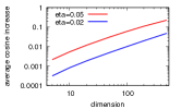
Figure 2: Expected increase in $\operatorname{\cos_{\text{sim}}}(\boldsymbol{f}_{1},\boldsymbol{f}_{2})$ as a function of dimension for $\boldsymbol{f}_{i}\sim\mathcal{N}^{d}$ after gradient update to same random context $\boldsymbol{c}\sim\mathcal{N}^{d}$

Consider two focus entities $1,2$ and corresponding examples $(1,j)$ and $(2,j)$. When the two examples are in the same focus-updating minibatch (where $\boldsymbol{c}_{j}$ is fixed) both $\operatorname{\cos_{\text{sim}}}(\boldsymbol{f}_{1},\boldsymbol{c})$ and $\operatorname{\cos_{\text{sim}}}(\boldsymbol{f}_{2},\boldsymbol{c})$ increase but a desirable side effect is that in expectation $\operatorname{\cos_{\text{sim}}}(\boldsymbol{f}_{1},\boldsymbol{f}_{2})$ increases as well. The updates are aligned also with full gradients but not with ind  arrangements that on average place corresponding examples half an epoch apart. Figure 2 shows the expected increase in cosine similarity $\mathbb{E}\left[\operatorname{\cos_{\text{sim}}}(\boldsymbol{f}^{\prime}_{1},\boldsymbol{f}^{\prime}_{2})-\operatorname{\cos_{\text{sim}}}(\boldsymbol{f}_{1},\boldsymbol{f}_{2})\right]\$ as a function of the dimension for example learning rates $\eta=0.02,0.05$ when the vectors $\boldsymbol{f}_{1}$, $\boldsymbol{f}_{2}$, and $\boldsymbol{c}$ are independently drawn from a product distribution $\mathcal{N}(0,1)^{d}$ of independent Gaussians.

Preservation of Jaccard similarities

We establish that coo arrangements preserve in expectation Jaccard similarities of pairs of rows and columns. The weighted Jaccard similarity of two vectors $\boldsymbol{v}$ and $\boldsymbol{u}$ is defined as

$$J(\boldsymbol{v},\boldsymbol{u})=\frac{\sum_{i}\min\{v_{i},u_{i}\}}{\sum_{i}\max\{v_{i},u_{i}\}}\ .$$ (3)

Lemma 4.3.

Consider a set of focus updating microbatches and let $X_{ij}$ be the random variable that is the multiplicity of example $(i,j)$. Then for any two rows $i,i^{\prime}$, the expectation of the empirical weighted Jaccard similarity on $X$ (when defined) is equal to the weighted Jaccard similarity on $\kappa$:

$$\mathbb{E}\left[J(X_{i\cdot},X_{i^{\prime}\cdot})\mid\sum_{j}\max\{X_{i^{\prime},j},X_{i,j}\}>0\right]=J(\kappa_{i,\cdot},\kappa_{i^{\prime},\cdot})$$

A symmetric claim holds for context updating microbatches.

Proof.

We consider a single microbatch and its contributions to the numerator and denominator of the empirical similarity $J(X_{i\cdot},X_{i^{\prime}\cdot})$. From Lemma 4.2, the possible contributions are $(0,0)$, $(0,1)$ or $(1,1)$. Therefore, $J(X_{i\cdot},X_{i^{\prime}\cdot})$ (if defined) is simply the average of the contributions to the numerator over microbatches that contributed to the denominator. The expectation of $J(X_{i\cdot},X_{i^{\prime}\cdot})$ (when defined) is therefore equal to the probability of a contribution to the numerator in a single microbatch given that there was a contribution to the denominator. If the shared context in the microbatch is $j$, the probability of contribution to the denominator is $\max\{\kappa_{i^{\prime},j},\kappa_{i,j}\}/\|\kappa_{\cdot j}\|_{\infty}$ and to the numerator is $\min\{\kappa_{i^{\prime},j},\kappa_{i,j}\}/\|\kappa_{\cdot j}\|_{\infty}$. The probability over the random draw of context $j$ of a contribution to the denominator and numerator respectively is $\sum_{j}\max\{\kappa_{i^{\prime},j},\kappa_{i,j}\}/\sum_{j}\|\kappa_{\cdot j}\|_{\infty}$ and $\sum_{j}\min\{\kappa_{i^{\prime},j},\kappa_{i,j}\}/\sum_{j}\|\kappa_{\cdot j}\|_{\infty}$. Since a contribution to the numerator is made only if there was one to the denominator, the expectation we seek is the ratio $J(\kappa_{i,\cdot},\kappa_{i^{\prime},\cdot})$. ∎

5 Refinement using LSH Maps

We provide methods to partition our coo microbatches so that they are smaller and of higher quality in the sense that a larger fraction of corresponding example pairs are between entities with higher similarity. To do this we use locality sensitive hashing (LSH) to compute randomized maps of entities to keys. Each map is represented by a vector $\mathbf{s}$ of keys for entities such that similar entities are more likely to obtain the same key. We use these maps to refine our basic microbatches by partitioning them according to keys.

Ideally, our LSH modules would correspond to the target similarity, but this creates a chicken-and-egg problem. Instead, we can use LSH modules that are available at the start of training and provide some proxy of the target similarity. For example, a partially trained or a weaker and cheaper to train model. We consider two concrete LSH modules based on Jaccard and on Angular LSH. The modules generate maps for either focus or context entities which are applied according to the microbatch designation. We will specify the map generation for focus entities, as maps for context entities can be symmetrically obtained by reversing roles.

Our Jaccard LSH module is outlined in Algorithm 4. The probability that two focus entities $i$ and $i^{\prime}$ are mapped to the same key (that is, $s_{i}=s_{i^{\prime}}$) is equal to the weighted Jaccard similarity of their association vectors $\kappa_{i\cdot}$ and $\kappa_{i^{\prime}\cdot}$ (For context updates the map is according to the vectors $\kappa_{\cdot j}$):

Lemma 5.1.

(Cohen et al., 2009)

$$\Pr[s_{i}=s_{i^{\prime}}]=J(\kappa_{ij},\kappa_{i^{\prime}j})$$

Our angular LSH module is outlined in Algorithm 5. Here we input an explicit “coarse” embedding $\tilde{\boldsymbol{f}}_{i},\tilde{\boldsymbol{c}}_{j}$ that we expect to be lower quality proxy of our target one. Each LSH map is obtained by drawing a random vector and then mapping each entity $i$ to the sign of a projection of $\tilde{\boldsymbol{f}}_{i}$ on the random vector. The probability that two focus entities have the same key depends on the angle between their coarse embedding vectors:

Lemma 5.2.

(Goemans & Williamson, 1995)

$$\Pr[s_{i}=s_{i^{\prime}}]=1-\frac{1}{\pi}\cos^{-1}\operatorname{\cos_{\text{sim}}}(\tilde{\boldsymbol{f}}_{i},\tilde{\boldsymbol{f}}_{i^{\prime}})\ ,$$

where $\operatorname{\cos_{\text{sim}}}(\boldsymbol{v},\boldsymbol{u}):=\frac{\boldsymbol{v}\cdot\boldsymbol{u}}{\|\boldsymbol{v}\|_{2}\|\boldsymbol{u}\|_{2}}$ is the cosine of the angle between the two vectors.

Multiple LSH maps can be applied to decrease microbatch sizes and increase the similarity level of entities placed in the same microbatch: With $r$ independent maps the probability that two entities are microbatched together is $\Pr[s_{i}=s_{i^{\prime}}]^{r}$ – thus the probability decreases faster when similarity is lower. The number of LSH maps we apply can be set statically or adaptively to obtain microbatches that are at most a certain size (usually the minibatch size). For efficiency, we precompute a small number of LSH maps in the preprocessing step and randomly draw from that set. The computation of each map is linear in the sparsity of $\kappa$.

foreach context $j$ do // i.i.d Exp distributed

      Draw $u_{j}\sim\operatorname{Exp}[1]$

foreach focus $i$ do // assign LSH bucket key

      $s_{i}\leftarrow\arg\min_{j}u_{j}/\kappa_{ij}$

return $\mathbf{s}$

Algorithm 4 Jaccard LSH map: Focus

Input: $\{\tilde{\boldsymbol{f}}_{i}\}$ // coarse $d$ dimensional embedding

Draw $r\sim S_{d}$ // Random vector from the unit sphere

foreach focus $i$ do // assign LSH bucket key

      $s_{i}\leftarrow\text{\bf{sign}}(r\cdot\tilde{\boldsymbol{f}}_{i})$

return $\mathbf{s}$

Algorithm 5 Angular LSH map: Focus

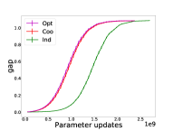
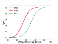
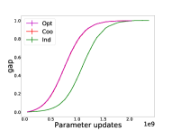
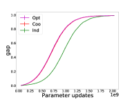
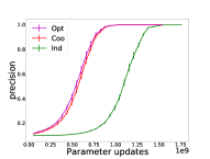
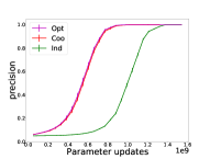
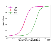
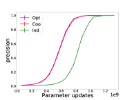
Figure 3: Cosine gap (top) and Precision at $k=10$ (bottom) with coo and ind arrangements and coo$+$OptLSH refinements in the course of training ($d=50$, $b=64$) for stochastic blocks with $B\in\{10,20,50,100\}$ (left to right).

6 Arrangement Methods Experiments

We trained embeddings with different arrangement methods: The baseline independent arrangements (ind) as in Algorithm 2, coordinated arrangements (coo) as in Algorithm 3, and some (coo$+$LSH) arrangements with Jaccard LSH. We also experimented with tunable arrangements (mix) that start with coo (which reaps much of its benefit earlier in training) and switch to coo$+$LSH or to ind. Finally, as another baseline we also trained using the more standard ind with two-sided updates. The results were similar or slightly inferior to one-sided ind and are reported in Appendix E.

6.1 Stochastic blocks data

We generated data sets using the stochastic blocks model (Condon & Karp, 2001). This synthetic data allowed us to explore the effectiveness of different arrangement methods as we vary the number and size of blocks. The simplicity and symmetry of this data (parameters, entities, and associations) allowed us to compare different arrangement methods while factoring out optimizations and methods geared for asymmetric data such as per-parameter learning rates or alterting the distribution of examples. The blocks data binary similarity allowed us to explore the limits of LSH refinements by refining coo microbatches according to ground truth similarity (partitioning coo microbatches by block membership) (coo$+$OptLSH).

The parameters for the generative model are the dimensions $n\times n$ of the matrix, the number of (equal size) blocks $B$, the number of interactions $r$, and the in-block probability $p$. The rows and columns are partitioned to consecutive groups of $n/B$, where the $i$th part of rows and $i$th part of columns are considered to belong to the same block. We generate the matrix by initializing the associations to be $\kappa_{ij}=0$. We then draw $r$ interactions independently as follows. We select a row index $i\in[n]$ uniformly at random. With probability $p$, we select (uniformly at random) a column $j\in[m]$ that is in the same block as $i$ and otherwise (with probability $1-p$) we select a column $j\in[n]$ that is outside the block of $i$. We then increment $\kappa_{ij}$. The final $\kappa_{ij}$ is the number of times $(i,j)$ was drawn. In our experiments we set $n=10^{4}$, $r=10^{7}$,$p=0.7$ and $B\in\{10,20,50,100\}$.

6.2 Implementation and methodology

We implemented our methods in Python using the TensorFlow library (Abadi & et al., 2015). We used the word embedding implementation of (Mikolov et al., 2013; word2vec.py, ) except that we used our methods to specify minibatches. The implementation included a default bias parameter associated with context embeddings and we trained embeddings with and without the bias parameter. The relative performance of arrangement methods was the same but the overall performance was significantly better when the bias parameter was used. We therefore report results with bias parameters. Details on training and prediction with bias are provided in Appendix D. We used a fixed learning rate to facilitate a more accurate comparison of methods and trained with $\eta=0.005$ to $\eta=0.15$. We observed similar relative performance and report results with $\eta=0.02$. We worked with minibatch size parameter values $b\in\{4,64,256\}$ (recall that $b$ is the number of positive examples and $\lambda=10$ negative examples are matched with each positive example), and embeddings dimension $d\in\{5,10,25,50,100\}$. Hyperparameter sweeps of $d$ and $b$ and the learning rate $\eta$ are reported respectively in Appendix A, Appendix B, and Appendix C.

6.3 Quality measures

We use two measures of the quality of an embedding with respect to the blocks ground truth. The first is the cosine gap which measures average quality and is defined as the difference in the average cosine similarity between positive examples and negative examples. We generate a sampled set $T_{+}$ of same-block pairs $(i,j)$ as positive test examples and a sampled set $T_{\_}$ of pairs that are not in the same block as negative test examples and compute

$$\frac{1}{|T_{+}|}\sum_{(i,j)\in T_{+}}\operatorname{\cos_{\text{sim}}}(\boldsymbol{f}_{i},\boldsymbol{c}_{j})-\frac{1}{|T_{-}|}\sum_{(i,j)\in T_{-}}\operatorname{\cos_{\text{sim}}}(\boldsymbol{f}_{i},\boldsymbol{c}_{j})\ .$$ (4)

We expect a good embedding to have high cosine similarity for same-block pairs and low cosine similarity for out of block pairs. The second measure we use, precision at $k$, is focused on the quality of the top predictions and is appropriate for recommendation tasks. For each sampled representative entity we compute the entities with top $k$ cosine similarity and consider the average fraction of that set that are in the same block.

#blocks		$0.75$		$0.95$		$0.99$
$B$	peak	%gain	$\times 10^{9}$	%gain	$\times 10^{9}$	%gain	$\times 10^{9}$
Cosine Gap Quality
10	1.09	31.07	1.58	24.80	1.89	19.06	2.17
20	1.03	29.56	1.40	23.74	1.72	18.13	1.97
50	1.00	25.52	1.22	20.46	1.55	14.73	1.80
100	0.99	20.66	1.09	15.27	1.40	12.11	1.64
Precision at $k=10$ Quality
10	1.00	43.64	1.12	37.70	1.24	37.41	1.38
20	1.00	40.80	1.03	36.16	1.14	33.47	1.23
50	1.00	33.89	0.92	31.37	1.04	25.35	1.09
100	1.00	26.67	0.84	23.37	0.94	20.00	1.02

Table 1: Training gain of coo with respect to ind baseline for stochastic blocks ($d=50$, $b=64$). Peak is maximum quality for coo. We report the training for ind to reach 75% , 95%, and 99% of peak with respective percent reduction in training with coo.

6.4 Stochastic blocks results

Our results were consistent for different dimensions and minibatch sizes and we report representative results for $d=50$ and $b=64$ and for the methods coo, ind, and the reference method coo$+$OptLSH. Results for the cosine gap quality measure and for the precision (at $k=10$) are reported in Figure 3 and Table 1. The figures show the increase in quality in the course of training for the different methods . The $x$-axis in these plots shows the amount of training in terms of the total number of gradient updates performed. The tables report the amount of additional training needed for ind to obtain the performance of coo. We observe that across all block sizes $B$ and for the two quality measures, coo arrangement resulted in significantly faster convergence than the ind arrangements. The gains were larger with larger blocks. Much of the gain of coo arrangements over ind was realized earlier in training and then maintained. The coo$+$OptLSH method provided only very modest improvement over coo and only for larger blocks. This improvement bounds that possible by any coo$+$LSH method on this data and indeed coo$+$LSH results (not shown) were between coo and coo$+$OptLSH.

6.5 Recommendation data sets and results

We performed experiments on two recommendation data sets, movielens1M and Amazon. The movielens1M dataset (Movielen1M, ) contains $10^{6}$ reviews by $6\times 10^{3}$ users of $4\times 10^{3}$ movies. The Amazon dataset (SNAP, ) contains $5\times 10^{5}$ fine food reviews of $2.5\times 10^{5}$ users on $7.5\times 10^{3}$ food items. Provided review scores were $[1\text{-}5]$ and we preprocessed the matrix by taking $\kappa_{ij}$ to be $1$ for review score that is at least $3$ and $0$ otherwise. We then reweighed entries in the movielens1M dataset by dividing the value by the sum of its row and column to the power of $0.75$. This is standard processing that retains only positive ratings and reweighs to prevent domination of frequent entities.

We created a test set $T_{+}$ of positive examples by sampling $20\%$ of the non zero entries with probabilities proportional to $\kappa_{ij}$. The remaining examples were used for training. As negative test examples $T_{-}$ we used random zero entries. We measured quality using the cosine gap and precision at $k=10$ over users with at least 20 nonzero entries. We used 5 random splits of the data to test and training sets and 10 runs per split. The results are reported in Figure 4 and Table 2. We show performance for coo and ind arrangements and also for a mix method that started out with coo arrangements and switched to ind arrangements at a point determined by a hyperparameter search. The mix method was often the best performer. We observe consistent gains of 3%-12% that indicate that arrangement tuning is an effective tool also on these more complex real-life data sets.

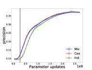
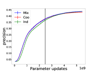
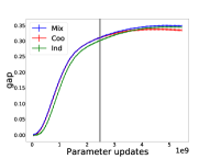
Figure 4: Precision at $k=10$ (left) and cosine gap (right) in the course of training with different arrangement methods on movielens1M(top) and Amazon(bottom) datasets. ($d=50$, $b=64$). The vertical lines indicate the switch point of mix (from coo to ind).

	$0.75\times$ peak		$0.95\times$ peak		$0.99\times$ peak
	%gain	$\times 10^{9}$	%gain	$\times 10^{9}$	%gain	$\times 10^{9}$
Amazon cosine gap: Gain over ind (peak=$0.35$)
Mix@4.5M	9.8	1.56	10.29	3.12	12.55	3.94
Coo	9.48	1.56	7.35	3.12	0	3.94
movielens1M cosine gap: Gain over ind (peak=$0.40)$
Mix@0.25M	11.94	0.68	7.45	0.82	6.08	0.92
Coo	11.94	0.68	4.97	0.82	6.08	0.92
Amazon precision: Gain over ind (peak=$0.44$)
Mix@4.5M	10.76	1.80	3.00	3.40	4.05	4.53
movielens1M precision: Gain over ind (peak=$0.37)$
Mix@0.25M	10.24	0.85	4.31	1.66	3.24	2.05

Table 2: Amazon and movielens1M, cosine gap and precision, training gain over ind baseline ($b=64$, $d=50$).

7 Example Selection Experiments

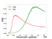
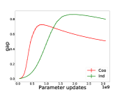
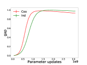
Figure 5: Training with selected examples (sub-epoch with ind and coo arrangements). Stochastic blocks datasets and minibatch size parameter $b=4$. Left to right: $(T=5,B=10)$; $(T=5,B=100)$, $(T=20,B=10)$, $(T=20,B=100)$.

In this section we empirically explore the qualities of the information contained in sub-epochs when using coo and ind arrangements. We select a small set of training examples that corresponds to sub-epochs with different arrangements and then train to convergence using multiple epochs on only the selected examples. We sampled $T=5,10,15,20$ examples from each row (for focus updates) and symmetrically from each column (for context updates) of the association matrix. To emulate a sub-epoch of ind arrangement, we select $T$ independent examples from each row $i$ by selecting a column $j$ with probability $\kappa_{ij}/\|\kappa_{i\cdot}\|_{1}$. To emulate a sub-epoch with coo arrangement we repeat the following $T$ times. We draw $u_{j}\sim\operatorname{Exp}[1]$ for each column and select for each row $i$ the column $\arg\max_{j}\kappa_{ij}/u_{j}$. Clearly the marginal distribution of both selections is the same: The probability that column $j$ is selected for row $i$ is equal to $\kappa_{ij}/\|\kappa_{i\cdot}\|_{1}$. Symmetric schemes apply to columns.

We trained embeddings (with no bias parameter and using ind arrangements) on these small subsets of examples using identical setups. Updates were according to minibatch designation: Row samples used for updating row embeddings and column samples for updating column embeddings. Representative results are reported in Figure 5. We observe that coo  selection consistently results in faster early training than ind selection but sometimes reaches a lower peak. We explain the faster early training by the coo selection preserving short-range similarities (based on first-hop relations) and the lower peak by lost “long-range” structure (that reflects longer-range relations as those captured by longer random walks and metrics such as personalized page rank). Our coo arrangements which use the complete set of examples retain both the short-range benefits of coo selections and the long-range benefits of ind selections.

8 Conclusion

We demonstrated that SGD can be accelerated with principled arrangements of training examples that are mindful of the “information flow” through gradient updates.

We mention some directions for followup work. Our arrangements respect a specified marginal distribution of training examples and hence can be combined and explored with methods, such as curriculum learning, that specify the distribution and even modify it in the course of training. We explored here one design goal of self similarity, where sub-epochs preserve structural properties of the full data. Our case study further focused on pairwise associations (“matrix factorization” with the SGNS objective), and preserving weighted Jaccard similarities of rows and columns. It is interesting to explore extensions that include other loss objectives and deeper networks and design principled arrangements suitable to more complex association structures.

Appendix A Embedding Dimension Sweep

We trained with different dimensions ($d=5$ to $d=200$) in order to understand the impact of the choice of dimension on final quality and convergence. We report results for ind arrangements as the relative behavior of arrangement methods was similar across dimensions with fixed training rate of $\eta=0.02$. The quality in the course of training (cosine gap and precision at $k=10$) is reported in Figure 6. For each experiment we report the training amount both in terms of the total number of parameter updates performed and the total multiplicity of positive examples processed during training. Note that the ratio of the number of updates to the multiplicity of examples is $\lambda d$, where $\lambda$ is the ratio of negative to positive examples and $d$ is the dimension. Therefore, the measures are linearly related for a fixed dimension but the number of updates per processed example increases with the dimension.

Amazon dataset

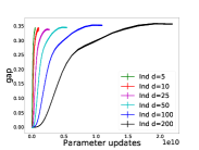
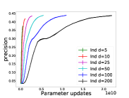
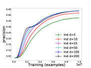
movielens1M dataset

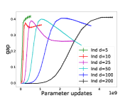
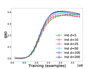
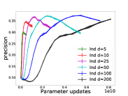
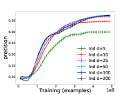
$10^{4}\times 10^{4}$ stochastic blocks dataset ($B=10$ blocks)

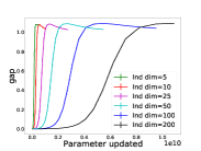
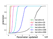
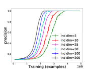
$10^{4}\times 10^{4}$ stochastic blocks dataset ($B=100$ blocks)

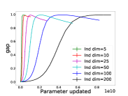
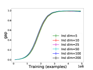
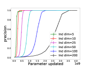
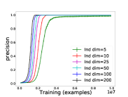
Figure 6: Training (ind with $b=64$) with different dimensions. Cosine gap and Precision for $k=10$ for movielens1M, Amazon, and stochastic blocks datasets. Training is reported in terms of number of parameter updates (left) and in terms of processed positive examples (right).

On all data sets we can observe slightly faster convergence with higher dimension in terms of number of training examples but generally slower convergence with dimension when considering the number of parameter updates. On the recommendations data sets and for the precision quality measure on the stochastic blocks data we can see that the peak quality increases with the dimension. This means that lower dimension is more effective in reaching a particular lower quality level but may reach lower peak quality. This supports methods (such as our LSH based refinements) that can leverage coarser, lower quality, but much more efficient to compute embeddings to accelerate the training of more complex models.

Appendix B Minibatch Size Sweep

We trained using ind arrangements with minibatches with size parameters $b=\{1,4,16,64,256\}$ in order to understand how performance depends on minibatch size. Recall that the parameter value $b$ is the number of positive examples, so the actual minibatch size in terms of the total number of examples is $\lambda b$, where $\lambda$ (we used $\lambda=10$) is the number of negative examples per postive one. When sweeping the minibatch size we used the learning rate $\eta=0.02$ and dimension $d=50$ as in our main experiments. On our synthetic and real datasets and both measures there was no performance difference between different parameters. Therefore, the gains of our arrangement methods hold also with respect to ind arrangements with very small minibatches.

Appendix C Learning Rate Sweep

We trained with a fixed learning rate to facilitate a better comparison of different arrangement methods and used $\eta=0.02$ in our reported results. Figure 7 shows the performance with ind arrangement for varied fixed learning rates between $\eta=0.01$ and $\eta=0.15$. As expected, we can see faster initial training with higher learning rate but (for the cosine gap measure) lower final quality. The relative behavior of different methods, in particular, the effectiveness of coo arrangements earlier in the training, was similar across learning rates. Figure 8 reports representative results for $\eta=0.01$.

Cosine gap
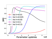
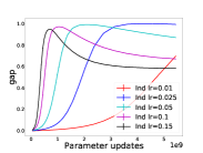
Precision at $k=10$

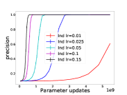
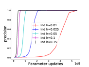
Figure 7: Cosine gap and Precision for $k=10$ with learning rate sweep (ind with $b=64$, $d=50$) for stochastic blocks with $B=10$ (left) and $B=100$ (right).

Cosine gap
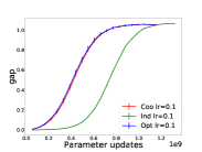
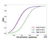
Precision at $k=10$

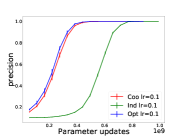
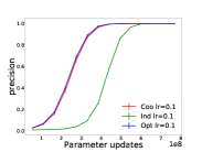
Figure 8: Cosine gap and precision with ind, coo, and coo$+$OptLSH arrangements with learning rate $\eta=0.01$ ($b=64$, $d=50$) for stochastic blocks with $B=10$ (left) and $B=100$ (right).

Appendix D Training with the Bias Parameter

The bias parameter can be viewed as an entry appended to embedding vectors, effectively increasing the dimension to $d+1$. The embedding $\boldsymbol{f}_{i}$ of focus entities is augmented by a fixed valued entry of $1$ and context embedding vectors $\boldsymbol{c}$ are augmented with a trainable bias parameter $b_{j}$.

When training with the bias parameter, we updated all parameters in one-sided manner as described, except that the bias terms (that can only be updated for context vectors) were updated in a two-sided manner. Specifically, in minibatches with context designations we update the bias term as the full context vector is updated. In minibatches with focus designation (where focus embeddings are updated) we also update the bias terms (only) of the context vectors. We maintain the way we match negative updates to positive updates on a per-parameter basis. When a bias term is updated (in a positive example) we balance it with $\lambda$ “antigravity” negative updates (only performed on the bias parameter) against a set of random focus vectors. Therefore, focus designated minibatches use a set of random context vectors for negative updates of focus embeddings and a set of random focus vectors for negative updates of bias terms of context embeddings.

When training we packed smaller same-designation microbatches into minibatches or partitioned large microbatches into consecutive minibatches. Without bias terms, with our one-sided updates the partitioning of a microbatches did not affect the end result as effectively all updates were independent. With bias terms on focus designations the updates are applied after each minibatch and were not independent. We found that applying all updates after each minibatch (instead of only applying them at the effective end of a microbatch) was generally helpful.

Following practice, when using embedding vectors in our cosine gap and precision performance measures we use the vectors without the bias terms. We confirmed that this practice yields smoother and better results also on our datasets. Moreover, for the precision measure we show results when seeking the closest context vector to a given focus vector. This way, the result is the same whether we use embedding vectors with the bias parameter or not. We confirmed that working this way (designating the context entity to be the one selected for a query focus entity) yields smoother and more accurate results.

Appendix E Two-sided Training

We used one-sided training to facilitate our coordinated arrangements and negative pairing and reported results with all arrangement methods, including the baseline ind, using one-sided training. For completeness, we report here respective results also with respect to the more standard baseline of independent arrangements with two-sided training.

Results are reported in Figure 9 for stochastic blocks data and in Figure 10 for the two recommendation datasets. The training cost ($x$-axis) is in terms of the total number of parameter updates performed, noting that two-sided training performs double the updates per example than one-sided training. We observe that two-sided ind performs very similarly and in some cases slightly worse than one-sided ind and therefore the training gains of our coordinated arrangements hold also with respect to the two-sided baseline.

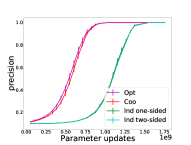
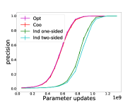
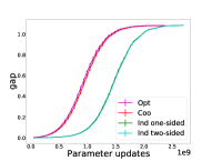
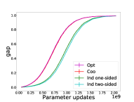
Figure 9: Precision at $k=10$ (top) and Cosine gap (bottom) with coo, coo$+$OptLSH, ind one-sided, and ind two-sided training ($d=50$, $b=64$) for stochastic blocks with $B\in\{10,100\}$.

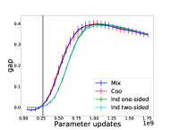
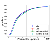
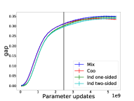
Figure 10: Precision at $k=10$ (left) and cosine gap (right) with coo, mix, and ind (one-sided and two-sided) arrangements on movielens1M(top) and Amazon(bottom) datasets. ($d=50$, $b=64$). The vertical lines indicate the switch point of mix (from coo to (one-sided) ind.

References

- Abadi & et al. (2015) Abadi, M. and et al. TensorFlow: Large-scale machine learning on heterogeneous systems, 2015. URL https://www.tensorflow.org/. Software available from tensorflow.org.
- Alain et al. (2015) Alain, G., Lamb, A., Sankar, C., Courville, A. C., and Bengio, Y. Variance reduction in SGD by distributed importance sampling. CoRR, abs/1511.06481, 2015. URL http://arxiv.org/abs/1511.06481.
- Bengio et al. (2009) Bengio, Y., Louradour, J., Collobert, R., and Weston, J. Curriculum learning. In ICML, 2009.
- Berry et al. (1995) Berry, M. W., Dumais, S. T., and O’Brien, G. W. Using linear algebra for intelligent information retrieval. SIAM Review, 37(4):573–595, 1995.
- Brewer et al. (1972) Brewer, K. R. W., Early, L. J., and Joyce, S. F. Selecting several samples from a single population. Australian Journal of Statistics, 14(3):231–239, 1972.
- Broder (2000) Broder, A. Z. Identifying and filtering near-duplicate documents. In Proc.of the 11th Annual Symposium on Combinatorial Pattern Matching, volume 1848 of LNCS, pp. 1–10. Springer, 2000.
- Bromley et al. (1994) Bromley, J., Guyon, I., Lecun, Y., Säckinger, E., and Shah, R. Signature verification using a "siamese" time delay neural network. In In NIPS Proc, 1994.
- Chopra et al. (2005) Chopra, S., Hadsell, R., and LeCun, Y. Learning a similarity metric discriminatively, with application to face verification. In 2005 IEEE Computer Society Conference on Computer Vision and Pattern Recognition (CVPR 2005), 2005.
- Cohen (1997) Cohen, E. Size-estimation framework with applications to transitive closure and reachability. J. Comput. System Sci., 55:441–453, 1997.
- Cohen (2014) Cohen, E. Distance queries from sampled data: Accurate and efficient. In KDD. ACM, 2014. full version: http://arxiv.org/abs/1203.4903.
- Cohen et al. (2009) Cohen, E., Kaplan, H., and Sen, S. Coordinated weighted sampling for estimating aggregates over multiple weight assignments. VLDB, 2, 2009. full version: http://arxiv.org/abs/0906.4560.
- Cohen (1980) Cohen, G. Auxiliary problem principle and decomposition of optimization problem. J Optim Theory Appl, 32, 1980.
- Condon & Karp (2001) Condon, A. and Karp, R. M. Algorithms for graph partitioning on the planted partition model. Random Struct. Algorithms, 18(2), 2001.
- Csiszar & Tusnády (1984) Csiszar, I. and Tusnády, G. Information geometry and alternating minimization procedures. Statistics & Decisions: Supplement Issues, 1, 1984.
- Deerwester et al. (1990) Deerwester, S., Dumais, S. T., Furnas, G. W., Landauer, T. K., and Harshman, R. Indexing by latent semantic indexing. Journal of the American Society for Information Science, 41(6):391–407, September 1990.
- Deng et al. (2009) Deng, J., Dong, W., Socher, R., Li, L.-J., Li, K., and Li, F.-F. Imagenet: A large-scale hierarchical image database. In In CVPR, 2009.
- Duchi et al. (2011) Duchi, J., Hazan, E., and Singer, Y. Adaptive subgradient methods for online learning and stochastic optimization. J. Mach. Learn. Res., 12, 2011. URL http://dl.acm.org/citation.cfm?id=1953048.2021068.
- Dumais (1995) Dumais, S. T. Latent semantic indexing (LSI): TREC-3 report. In Harman, D. K. (ed.), The Third Text Retrieval Conference (TREC-3), pp. 219–230, Gaithersburg, MD, 1995. U. S. Dept. of Commerce, National Institute of Standards and Technology.
- Fu & Zhang (2017) Fu, T. and Zhang, Z. Cpsg-mcmc: Clustering-based preprocessing method for stochastic gradient mcmc. In AISTATS, 2017.
- Gemulla et al. (2011) Gemulla, R., Nijkamp, E., Haas, P. J., and Sismanis, Y. Large-scale matrix factorization with distributed stochastic gradient descent. In ACM KDD 2011. ACM, 2011.