Complex activity patterns generated by short-term synaptic plasticity

Abstract

Short-term synaptic plasticity (STSP) affects the efficiency of synaptic transmission for persistent presynaptic activities. We consider attractor neural networks, for which the attractors are given, in the absence of STSP, by cell assemblies of excitatory cliques. We show that STSP may transform these attracting states into attractor relics, inducing ongoing transient-state dynamics in terms of sequences of transiently activated cell assemblies, the former attractors. Subsequent cell assemblies may be both disjoint or partially overlapping. It may hence be possible to use the resulting dynamics for the generation of motor control sequences.

1 Introduction

Changes in the transmission properties of synapses lead to a modulation of information processing. Synaptic plasticity, which is present on many time scales, is responsible, for learning and computational processes [1], as well as for memory consolidation [2] and motor pattern generation [3]. Short-term synaptic plasticity (STSP) contributes, in this context, to the regulation of brain networks on time scales ranging typically from tens of milliseconds to seconds [4]. It is affected, in the standard Tsodyks-Markram model [5, 2, 1], by two factors: a reservoir $\varphi(t)$ of neurotransmitter vesicles and the Ca-concentration, $u(t)$, which in turn influences the release probability of vesicles. The synaptic efficiency is then proportional to the number of released neurotransmitters per incoming presynaptic spike, which is, in turn, proportional to both $u$ and $\varphi$.

2 Methods and results

We consider a modified version of the original Tsodyks-Markram model for presynaptic plasticity:

$$\begin{aligned} \dot{u}&={\left(U(y)-u\right)}/{T_{u}}\qquad\qquad&U(y)&=1+(U_{\text{max}}-1)y\nu\\ \dot{\varphi}&={\left(\Phi(y,u)-\varphi\right)}/{T_{\varphi}}\qquad\qquad&\Phi(y,u)&=1-{uy\nu}/{U_{\text{max}}}\end{aligned}~{}.$$ (1)

$T_{u}$ and $T_{\varphi}$ set here the relaxation times respectively for the Ca-concentration $u$ and for the vesicle level $\varphi$. The target functions $U(y)$ and $\Phi(y,u)$ depend, in addition, on the level $y\in[0,1]$ of the presynaptic firing rate. The parameter $\nu=1/0$ is used as a switch, turning STSP on/off. The synaptic variables return to their baseline values, $u,\varphi\rightarrow 1$, for both $\nu=0$ and $y=0$.

The model defined by (1) allows the reservoir of neurotransmitter to fully deplete, $\varphi\rightarrow 0$, for sustained presynaptic activity $y=1$, and for a direct control of the maximal Ca-concentration, $U_{\text{max}}$. Note that STSP influences synaptic transmission only transiently, its effects are hence fading away in the absence of presynaptic neural activity, viz for $y=0$.

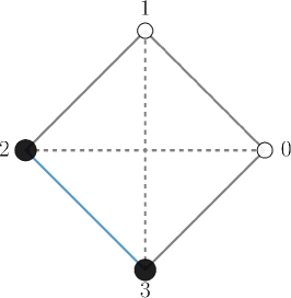
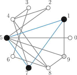
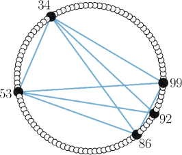
Figure 1: Networks of $N=4/10/100$ neurons (left/middle/right) with one active clique (black nodes and blue lines). Shown are the connections (both types/only excitatory/of the active clique). Active/inactive nodes are indicated by filled/open numbered circles and excitatory/inhibitory links by continuous/dashed lines.

2.1 Transient-state dynamics with clique encoding

We use the full depletion model, defined by Eq. (1), to generate transient-state dynamics [6], analogously to the method introduced in [7], in attractor neural networks of different size. The network structures consist of all-to-all bidirectional couplings, with static excitatory connections $w_{jk}$, and transiently changing inhibitory connections of effective synaptic weights $z_{jk}u_{k}\varphi_{k}$. Excitatory and inhibitory couplings are mutually exclusive, $w_{jk}z_{jk}=0$, self-connections are excluded.

The topology of the considered networks is sketched in Fig. 1. The $N=4$ site network has $w_{jk}=w_{kj}=w_{0}$ and $z_{jk}=z_{kj}=z_{0}$, implying a $C_{4}$ rotational symmetry. The excitatory connections form a ring, allowing two independent inhibitory links. In case of the other two networks of $N=10$ and $N=100$ neurons, first an Erdős-Rényi network of excitatory links is generated, with $w_{ij}=w_{0}+\eta^{w}_{ij}$, using a connection probability $p=0.3$. The $z_{ij}=z_{0}+\eta^{z}_{ij}$ are then complementary (not explicitly shown). $\eta^{w}_{ij}$ and $\eta^{z}_{ij}$ are here normal distributed random variables with respective standard deviations $w_{\text{std}}$ and $z_{\text{std}}$.

We consider networks of simple rate-encoding neurons, with a sigmoidal transfer function $y(x)=1/(1+e^{-ax})$, where $x$ plays the role of the membrane potential. The dynamics of the neural activity $y_{k}=y(x_{k})$ is defined by:

$$\dot{x}_{j}=-\Gamma x_{j}+\sum_{k=0}(w_{jk}y_{k}+z_{jk}u_{k}\varphi_{k}y_{k})+I\,,\qquad\quad j,k\in\{0,\dots,N-1\}$$ (2)

together with the STSP rules (1). $x_{j}$ denotes the membrane potential of the $j$-th neuron and $I$ a constant global input (as generated by other brain regions). $\Gamma$ is here the relaxation rate of the leak term.

The parameters are set such that the system defined by (2) has stable fixpoints when STSP is absent ($\nu=0$), characterized in turn by active cell assemblies of excitatory cliques of neurons (as highlighted in Fig. 1 by black nodes and blue links). These cell assemblies realize a particular form of information encoding in the brain, called as clique encoding [7]. STSP with $\nu=1$ destabilizes the fixpoint attractors, leading to transient-state dynamics corresponding to stable limit cycles, or chaotic attractors, in the full $3N$ dimensional phase space.

As an example we present in Fig. 2, two limit cycle solutions of the $N=4$ site symmetric network. In the first case a synchronous switching of active pairs of neurons is observed. This flip-flop dynamics (class I.) breaks the $C_{4}$ symmetry of the network spontaneously. The second, a travelling wave solution (class II.), is characterized by an activity bump [8], which may travel clock or counter-clock wise. There are $2$ and $4$ equivalent solutions respectively for the flip-flop state and for the travelling wave.

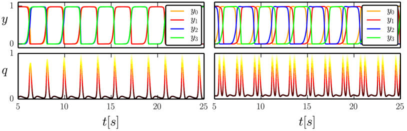
Figure 2: The neural activity $y$ (top) of the $N=4$ neuron symmetric network with STSP, $\nu=1$, and the corresponding normalized speed $q$, see Eq. (3), of the flow (bottom). Two examples of limit cycle solutions are shown, with switching (left) and travelling wave (right) dynamics. The parameters are $\Gamma=10\,\text{s}^{-1}$, $T_{u}=300\,\text{ms}$, $T_{\varphi}=600\,\text{ms}$, $w_{0}=40\,\text{Hz}$, $z_{0}=-100\,\text{Hz}$, $U_{\text{max}}=4$, $a=1$, $\nu=1$ and $I=0$.

The trajectory revisits repeatedly the destabilized fixpoints, slowing down in their neighborhood. To quantify this behavior, we use the normalized speed $q$ of the flow in the phase-space [9], as defined by:

$$q=Q/Q_{\text{max}}\,,\qquad Q=\lvert\mathbf{f}(\mathbf{v})\rvert^{2}\,,\qquad\quad\dot{\mathbf{v}}=\mathbf{f}(\mathbf{v})\,,$$ (3)

with $\mathbf{v}=(\mathbf{x},\mathbf{u},\boldsymbol{\varphi})$ and with $\mathbf{f}$ denoting the right-hand side function of the differential equation. The normalization is done with respect to the maximal flow speed $Q_{\text{max}}$ of the respective limit cycle. The normalized speed $q$ peaks, as shown in Fig. 2, at the transition points, being close to zero when the cell assemblies are transiently activated.

Note that due to the phase space contraction, $\nabla\cdot\mathbf{f}<0$, the transient-state dynamics is always realized by stable limit-cycle or chaotic attractors.

2.2 Bifurcation analysis of the symmetric network

We consider first the $N=4$ site symmetric network, as a function of the $I$, the global input, as it allows for a detailed bifurcation analysis of the system. Central sections of the bifurcation diagram, created with PyDSTool [10], are presented in Fig. 3.

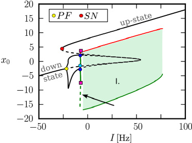
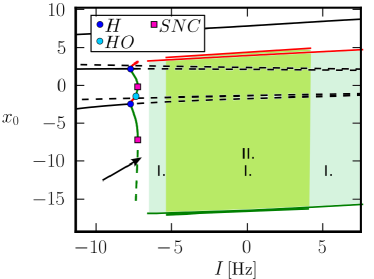
Figure 3: Left: Bifurcation diagram of the $N=4$ neuron network, projected on $x_{0}$, as a function of the input current $I$. Right: A blow-up for the region with Hopf-bifurcations. Notations: solid black lines - stable fixpoints, dashed black lines - unstable fixpoints, red/green solid (dashed) lines - maximal/minimal amplitudes of stable (unstable) cycles, $PF$ - Pitchfork, $SN$ - saddle-node, $H$ - supercritical Hopf, $HO$ - homoclinic, and $SNC$ - saddle-node bifurcation of limit cycles. Different shades of green denote parameter intervals of class I. and II. transient-state dynamics. The arrow points to a chaotic window. The parameters are the same as for Fig. 2.

The symmetric network has $4$ stable fixpoints in the absence of STSP ($\nu=0$), corresponding to active two-neuron cliques. Thanks to the $C_{4}$ symmetry, there exists a fifth, unstable state as well, for which all four neurons have the same activity $y^{*}_{j}\approx 0.3$, $j\in\{0,1,2,3\}$. This symmetric solution splits up into three fixpoints for a large range of input values $I$ when STSP is turned on ($\nu=1$). This can be seen by solving graphically the fixpoint equation,

$$\Gamma x^{*}=\left(2w_{0}+z_{0}u^{*}\varphi^{*}\right)y^{*}+I\,,\quad u^{*}=1+(U_{\text{max}}-1)y^{*}\,,\quad\varphi^{*}=1-u^{*}y^{*}/U_{\text{max}}$$

where $x^{*}_{j}=x^{*}$, $u^{*}_{j}=u^{*}$, $\varphi^{*}_{j}=\varphi^{*}$ and $y(x^{*})=y^{*}$, for $j\in\{0,1,2,3\}$. The two new fixpoints are generally referred to as up- and down-states [1], with all neurons being nearly active $y_{j}\approx 1$, or inactive $y_{j}\approx 0$. This ”S-shaped” fixpoint solution forms the skeleton of the bifurcation diagram presented in Fig. 3. The up-state is found to be stable in the considered parameter range even for certain negative inputs, being annihilated in the end by a saddle-node bifurcation ($SN$). The down-state splits, on the other hand, into four clique-encoding solutions (seen as two branches, due to the $C4$ symmetry) via a higher order Pitchfork bifurcation ($PF$), leaving the original state unstable.

For increasing input values of $I$ we find a cascade of bifurcations (akin to the series found in [11]), leading ultimately to transient-state dynamics type limit cycles. This cascade involves supercritical Hopf bifurcations ($H$), saddle-node bifurcation of cycles ($SNC$), and homoclinic bifurcation $HO$.

We also found a narrow chaotic window (indicated by the arrow in Fig. 3), which we however did not examine in detail. The collapse of the chaotic attractor for larger inputs leads to class I. limit cycles (light green). Class II. travelling wave cycles (dark green) coexist with the flip-flop solutions, having very similar amplitudes (oscillating between the upper red and lower green lines) in the $x_{0}$ projection. As already discussed, the trajectories slow down, in both cases, close to the destabilized clique-fixpoints (dashed lines developing out of the Hopf points).

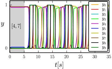
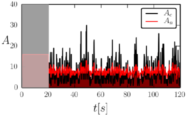
Figure 4: Left: Time-series of firing rates $y_{k}$ of the $N=10$ site random network. Right: Chaotic-like dynamics of the $N=100$ site network, showing the number of active neurons and cliques, $A_{n}$ and $A_{c}$ respectively, as a function of time. STSP is turned off in the first $5/20$ seconds (left/right), as indicated by the respective grey-shaded areas, with $A_{c}=1/41$ and $A_{n}=2/16$ initially (left/right). The parameters are $I=0$, $a=0.4$, $\Gamma=10\,\text{s}^{-1},$ $T_{u}=21\,\text{ms}$, $T_{\varphi}=706\,\text{ms}$, $\sigma_{w}=\sigma_{z}=10\,\text{Hz}$, together with $w_{0}=80\,\text{Hz}$, $z_{0}=-200\,\text{Hz}$ for the $N=10$ site, and $w_{0}=100\,\text{Hz}$, $z_{0}=-100\,\text{Hz}$ for the $N=100$ site networks.

2.3 Complex activity patterns generated by random networks

Considering larger networks, we show in Fig. 4 that transient-state dynamics emerges generically out of fixpoint states when STSP is turned on. The sequence of activity patterns generated by STSP ($\nu=1$) then visits consecutively a subset of the fixpoints present at $\nu=0$, giving rise to multiple coexisting limit cycles and/or chaotic attractors.

The time series of firing rates of the $N=10$ site network shown in Fig. 4 is, to give an example:

$[4,7]\rightarrow[1,5,7]\rightarrow[1,5,9]\rightarrow[5,8,9]\rightarrow[6,8]\rightarrow[3,6]\rightarrow[3,4]\rightarrow\,,$

where we have identified cliques by the indices $k$ of the activated neurons (defined by $y_{k}>0.9$). For the selected parameters another limit cycle, $[1,5,7]\rightarrow[1,5,9]\rightarrow[5,8,9]\rightarrow[1,5,9]\rightarrow[1,5,7]$, with a complementary basin of attraction, in terms of initial states, exists. Defining with $A_{n}$ and $A_{c}$ the number of activated neurons and cliques respectively, we find that $A_{n}=2,3$ and $A_{c}=1$ during the cycle of the $N=10$ site shown in Fig. 4.

The number of co-activated cliques $A_{c}$ is controlled by the ratio of the average excitatory and inhibitory weights $w_{0}/|z_{0}|$, as shown by the data for the $N=100$ site network presented in Fig. 4 (for which $w_{0}/|z_{0}|=1$). The initial state with turned off STSP corresponds to cell assemblies formed by multiple cliques, $A_{c}=\nobreak 40$, with $A_{n}=16$ active neurons. The transient synaptic plasticity generates, furthermore, chaotic-like dynamics, with highly variable clique constellations, and a average network activity of $\langle A_{n}/N\rangle\approx 8\%$, a biologically realistic scenario.

3 Conclusions

We have investigated here the effect of a ubiquitous form of transient synaptic plasticity, STSP, on the dynamics of attractor neural networks. We find that STSP generically transforms stable attractors into attractor relics, inducing ongoing transient-state dynamics in terms of alternating sequences of active cell assemblies. We hence believe that it is essential to include STSP, which operates on time scales of 0.1-1.0 seconds, in studies of biologically inspired neural networks. Applications range from working memory implementations [2] to generation of motor control patterns by neural networks [1, 3].

References

- [1] Cortes et al. Short-term synaptic plasticity in the deterministic tsodyks-markram model leads to unpredictable network dynamics. Proceedings of the National Academy of Sciences, 110(41):16610–16615, 2013.
- [2] Gianluigi Mongillo, Omri Barak, and Misha Tsodyks. Synaptic theory of working memory. Science (New York, N.Y.), 319(5869):1543–6, 2008.
- [3] Laura Martin, Bulcsú Sándor, and Claudius Gros. Closed-loop robots driven by short-term synaptic plasticity: Emergent explorative vs. limit-cycle locomotion. Frontiers in Neurorobotics, 10:12, 2016.
- [4] Anirudh Gupta, Yun Wang, and Henry Markram. Organizing principles for a diversity of GABAergic interneurons and synapses in the neocortex. Science, 287(5451):273–278, jan 2000.
- [5] Misha Tsodyks, K Pawelzik, and Henry Markram. Neural networks with dynamic synapses. Neural computation, 835(1996):821–835, 1998.
- [6] Misha Rabinovich, Ramon Huerta, and Gilles Laurent. Transient dynamics for neural processing. Science (New York, N.Y.), 321(5885):48–50, 2008.
- [7] Claudius Gros. Neural networks with transient state dynamics. New Journal of Physics, 9(4):109–109, 2007.
- [8] Lawrence Christopher York and Mark C W van Rossum. Recurrent networks with short term synaptic depression. Journal of computational neuroscience, 27(3):607–20, 2009.
- [9] David Sussillo and Omri Barak. Opening the black box: low-dimensional dynamics in high-dimensional recurrent neural networks. Neural computation, 25(3):626–49, 2013.
- [10] Robert Clewley. Hybrid models and biological model reduction with pydstool. PLoS computational biology, 8(8):e1002628, 2012.
- [11] Bulcsú Sándor and Claudius Gros. A versatile class of prototype dynamical systems for complex bifurcation cascades of limit cycles. Scientific Reports, 5:12316, 2015.