Volumes of 3-ball quotients as intersection numbers

Abstract.

We give an explicit description of the 3-ball quotients constructed by Couwenberg-Heckman-Looijenga, and deduce the value of their orbifold Euler characteristics. For each lattice, we also give a presentation in terms of generators and relations.

1. Introduction

Let $X=G/K$ be an irreducible symmetric space of non-compact type. It is a well known fact originally due to Borel [4] that $G$ contains lattices, i.e. discrete subgroups such that $\Gamma\backslash X$ has finite volume. In fact, $\Gamma$ can be chosen so that $\Gamma\backslash X$ is compact or non-compact.

The standard construction of lattices comes from arithmetic, as we briefly recall. Take a linear algebraic group $H$ defined over $\mathbb{Q}$, and denote by $H^{0}_{\mathbb{R}}$ the connected component of the identity in the group of real points $H_{\mathbb{R}}$. Assume that there is a surjective homomorphism $\varphi:H^{0}_{\mathbb{R}}\rightarrow G$ with compact kernel, and consider the group $\Gamma=\varphi(H^{0}_{\mathbb{R}}\cap H_{\mathbb{Z}})$. It is a standard fact that $\Gamma$ is then a lattice in $G$ (this is essentially a result by Borel and Harish-Chandra [5]).

By definition, a lattice $\Gamma^{\prime}$ in $G$ is called arithmetic if there exists $H,\varphi,\Gamma$ as above such that $\Gamma$ and $\Gamma^{\prime}$ are commensurable in the wide sense, i.e. possibly after replacing $\Gamma$ by $g\Gamma g^{-1}$ for some $g\in G$, the intersection $\Gamma\cap\Gamma^{\prime}$ has finite index in both $\Gamma$ and $\Gamma^{\prime}$. It follows from important work of Margulis [21], Corlette [8], Gromov-Schoen [17] that if $X$ is not a real or complex hyperbolic space, then every lattice in $G$ is actually arithmetic.

In the case $X=H^{n}_{\mathbb{R}}$, $G=PO(n,1)$, several constructions of non-arithmetic lattices are known, but no general structure theory for lattices has been worked out. It follows from a construction of Gromov and Piatetski-Shapiro [16] that there exist non-arithmetic lattices in $G$ for arbitrary $n\geqslant 2$, and that there are infinitely many commensurability classes in each dimension.

The case $X=H^{n}_{\mathbb{C}}$, $G=PU(n,1)$ is even further from being understood. There is currently no generalization of the Gromov-Piatetski-Shapiro construction to the complex hyperbolic case, and in fact (for $n>2$) only finitely many commensurability classes of non-arithmetic lattices are known, only in very low dimension; there are currently 22 known classes in $PU(2,1)$, see [14], and 2 known classes in $PU(3,1)$ see [11].

The first examples were constructed by Mostow [24], generalized by Deligne-Mostow [10], then the list was expanded [15], [14], [11]. Some recent constructions rely on the use of fundamental domains (and heavy computational machinery), but most examples have been given alternative constructions using orbifold uniformization (see [12], [13]).

It turns out most known examples are in fact in a list of lattices that was produced by Couwenberg, Heckman and Looijenga [9] (their list contains representatives of 17 out of the 22 classes in $PU(2,1)$, and both classes in $PU(3,1)$). For the sake of brevity, we refer to their lattices as CHL lattices, and to the corresponding quotients as CHL ball quotients.

An explicit description of the quotient of all the 2-dimensional CHL lattices can be obtained by combining the results in [10] and [12]. The goal of this paper is to give an explicit description of the quotient for all 3-dimensional CHL lattices. In principle a similar description can of course be worked out for higher-dimensional examples (recall that CHL lattices only exist in dimension at most 7).

Using this description, we compute orbifold Euler characteristics of the 3-dimensional CHL ball quotients. Recall that the orbifold Euler characteristic is a universal multiple of the volume, namely

$$Vol(\Gamma\backslash\mathbb{B}^{n})=\frac{(-4\pi)^{n}}{(n+1)!}\chi^{orb}(\Gamma\backslash\mathbb{B}^{n}),$$

if the metric is normalized to have holomorphic sectional curvature $-1$ (this is an orbifold version of the Chern-Gauss-Bonnet formula, see [29]).

Since most of these lattices are arithmetic, one could in principle compute their covolumes by using the Prasad formula [27] (for all but one lattice, namely the non-arithmetic one). Note however that Prasad’s formula gives the covolume of a specific lattice in each commensurability class (the so-called principal arithmetic lattices); unfortunately the relation of a given lattice to the principal arithmetic lattice in its commensurability class can be difficult to make explicit. In fact, our volume computations should make it possible to relate arithmetic CHL lattices to the corresponding principal arithmetic groups in their commensurability class. It may also be useful in order to distinguish commensurability classes of non-arithmetic lattices, using the Margulis commensurator theorem and volume estimates, in the spirit of the arguments in [14].

Note that volumes of Deligne-Mostow ball quotients (which are special cases of CHL lattices) were already known. They were computed by McMullen [22] using a very different computation; and by Koziarz and Nguyen [20] in a computation which is closer in spirit to ours, since they compute intersection numbers.

More specifically, in our paper, the orbifold Euler characteristics are obtained by identifying the quotients as pairs $(X,\Delta)$ where $X$ is an explicit normal space birational to the quotient of $\mathbb{P}^{n}$ by a finite group, and $\Delta$ is an explicit $\mathbb{Q}$-divisor in $X$. We then compute

(1) $$\frac{1}{(n+1)^{n-1}}c_{1}^{orb}(X,\Delta)^{n}=\frac{(-1)^{n}}{(n+1)^{n-1}}(K_{X}+\Delta)^{n},$$

which is equal to $c_{n}^{orb}(X,\Delta)$ (and the latter is equal to the orbifold Euler characteristic). Indeed, by Hirzebruch proportionality [18], the ratios of Chern numbers for ball quotients must be the same as those of the compact dual symmetric space $\mathbb{P}^{n}$, and we have $c_{1}(\mathbb{P}^{n})=nH$, $c_{n}(\mathbb{P}^{n})=(n+1)H^{n}$ (where $H$ denotes the hyperplane class). We will only use the case $n=3$, where the relevant formula reads $c_{1}^{orb}(X,\Delta)^{3}=16c_{3}(X,\Delta)$.

Note that we do not compute the orbifold Euler characteristic directly, which can be done by using the stratification of $X$ by strata with constant isotropy groups (see [29] or [22]). Indeed, such a computation would require a lot of bookkeeping (especially in cases where the relevant ball quotient is obtained from $\mathbb{P}^{3}$ by blowing-up and then contracting, see section 3).

Strictly speaking, the above description is only valid for compact ball quotients. In terms of the notation in [9], cocompactness corresponds to the fact that $\kappa_{L}\neq 1$ for every irreducible mirror intersection $L$ in the arrangement. On the other hand, the formulas we use for cocompact lattices remain valid for non-cocompact ones, since the volume of the complex hyperbolic structures constructed by Couwenberg, Heckman and Looijenga depend continuously (in fact even analytically) on the deformation parameter (see Theorem 3.7 in [9]).

Our computations depend on detailed properties of the combinatorics of the hyperplane arrangements given by the mirrors in 4-dimensional Shephard-Todd groups. We list these combinatorial properties in section 7 in the form of tables, since we could not find all of it in the literature (the data can be gathered fairly easily using modern computer technology).

For concreteness, we also give explicit presentations for the 3-dimensional CHL lattices in terms of generators and relations, see section 6. The fact that one can work out explicit presentations was already mentioned by Couwenberg, Heckman and Looijenga (see Theorem 7.1 in [9]). This depends on the knowledge of the presentations for braid groups that were worked out by Broué, Malle, Rouquier [6], Bessis and Michel [3], and fully justified thanks to later work by Bessis [2].

We hope that our paper provides useful insight into the beautiful paper by Couwenberg, Heckman and Looijenga.

Acknowledgements: It is a pleasure to thank Stéphane Druel for many useful conversations related to this paper. I also thank John Parker for his suggestion to use algebro-geometric methods to compute volumes of CHL lattices. I am also very grateful to the referee, who made many suggestions to improve the paper.

2. Finite unitary groups generated by complex reflections

In this section, we briefly recall the Shephard-Todd classification of finite unitary groups generated by complex reflections, see [30] (see also [7] or [6]).

2.1. Complex reflections

Recall that a complex reflection in $V=\mathbb{C}^{n}$ is a diagonalizable linear transformation whose eigenvalues are $1,\dots,1,\zeta$ for some complex number $\zeta\neq 1$ with $|\zeta|=1$ (the eigenvalue 1 has multiplicity $n-1$). A group is called a complex reflection group if it is generated by complex reflections, and it is called unitary if it preserves a Hermitian form on $V$.

Complex reflections preserving a Hermitian inner product $\langle v,w\rangle=w^{*}Hv$ can be written as $R_{v,\zeta}$ where

$$R_{v,\zeta}(x)=x+(\zeta-1)\frac{\langle x,v\rangle}{\langle v,v\rangle}v$$

for some nonzero vector $v\in V$. The fixed point set of $R_{v,\zeta}$ in $V$ then consists of the orthogonal complement $v^{\perp}$ with respect to $H$, and it is called the mirror of $R_{v,\zeta}$. The number $\zeta$ is called the multiplier of $R_{v,\zeta}$ and the argument of $\zeta$ is called the angle of $R_{v,\zeta}$.

We will often assume that the multiplier $\zeta$ is a root of unity (which is needed if we are to consider only finite groups), and even that $\zeta=e^{2\pi i/p}$ for some natural number $p\geqslant 2$ (which can be assumed by replacing the reflection by a suitable power).

2.2. Braid relations

Let $G$ be a group, and let $a,b\in G$. We say that $a,b$ satisfy a braid relation of length $k$ if

(2) $$(ab)^{k/2}=(ba)^{k/2}.$$

When $k$ is odd, $(ab)^{k/2}$ stands for a product of the form $aba\cdots ba$ with $k$ factors (and similarly for $(ba)^{k/2}$). We write ${\rm br}_{k}(a,b)$ for the relation of equation (2).

Of course, ${\rm br}_{1}(a,b)$ is equivalent to $a=b$, and ${\rm br}_{2}(a,b)$ means that $a$ and $b$ commute. The relation ${\rm br}_{3}(a,b)$, i.e. $aba=bab$ is often called the standard braid relation. If ${\rm br}_{k}(a,b)$ holds, but ${\rm br}_{j}(a,b)$ does not hold for any $j<k$, we write ${\rm br}(a,b)=k$.

2.3. Coxeter diagrams

It is customary to describe complex reflection groups (with a finite generating set of reflections) by a Coxeter diagram, which is a labelled graph. The set of nodes in the graph is given by a generating set of complex reflections, and each node consists of a circled integer, corresponding to the order of the corresponding complex reflection (more precisely, a circled $p$ stands for a complex reflection of angle $\frac{2\pi}{p}$).

The nodes in the Coxeter diagram, corresponding to reflections $a$ and $b,$ are joined by an edge labelled by a positive integer $k$ if the braid relation ${\rm br}_{k}(a,b)$ holds (see 2.2). Moreover, by convention:

• when ${\rm br}_{2}(a,b)$, the edge is not drawn,

• when ${\rm br}_{3}(a,b)$, the label 3 is omitted and the corresponding edge is drawn without any label,

• when ${\rm br}_{4}(a,b)$, the label 4 is omitted and the corresponding edge is drawn as a double edge.

Beware that a given complex reflection group can be represented by several Coxeter diagrams (since there can be several non-conjugate generating sets of reflections), and in general a Coxeter diagram need not represent a unique group (even up to conjugation in $GL(V)$).

2.4. The Shephard-Todd classification

Let $G$ be a group acting irreducibly on $V=\mathbb{C}^{n}$. If $G$ has an invariant Hermitian form on $V$, then that form is unique. If we assume further that $G$ is finite, then any invariant Hermitian form must be definite, so we can think of $G$ as a subgroup of $U(n)$.

Finite subgroups of $U(n)$ generated by complex reflections were classified by Shephard-Todd in [30]. It is enough to classify irreducible groups, which come in three infinite families (symmetric groups, imprimitive groups $G(m,p,n)$ and groups generated by a single root of unity), together with a finite list of groups.

The infinite families occur in the Shephard-Todd list as $G_{1},G_{2}$ and $G_{3}$, and the finite list contains groups $G_{4}$ through $G_{22}$ (in dimension 2), $G_{23}$ through $G_{27}$ (in dimension 3), $G_{28}$ through $G_{32}$ (in dimension 4), $G_{33}$ (in dimension 5), $G_{34}$ and $G_{35}$ (in dimension 6), $G_{36}$ (in dimension 7), and $G_{37}$ (in dimension 8). The list is given on p.301 of [30].

2.5. Presentations for Shephard-Todd groups and for the associated braid groups

Presentations for these groups in terms of generators and relations are listed in section 11 of [30]. It can be useful to have reflection presentations, i.e. presentations such that the generators correspond to complex reflections in the group. Coxeter diagrams for reflection presentations can be found in convenient form in pp.185–188 of [6]; some diagrams have extra decorations, since the braid relations between generators do not always suffice. For instance, the diagram for the group $G_{31}$ is the one given in Figure 1.

Figure 1. The Coxeter diagram for $G_{31}$

This diagram gives a presentation of the form

$$\langle\quad r_{1},r_{2},r_{3},r_{4},r_{5} | r_{1}^{2},r_{1}r_{5}r_{4}=r_{5}r_{4}r_{1}=r_{4}r_{1}r_{5}$$

$${\rm br}_{3}(r_{1},r_{2}),{\rm br}_{3}(r_{2},r_{5}),{\rm br}_{3}(r_{5},r_{3}),{\rm br}_{3}(r_{3},r_{4}),[r_{1},r_{3}],[r_{2},r_{3}],[r_{2},r_{4}]\quad\rangle$$

where all braid and commutation relations are dictated by the general Coxeter description, and the circle joining the nodes for $r_{1}$, $r_{5}$ and $r_{4}$ stands for the relations $r_{1}r_{5}r_{4}=r_{5}r_{4}r_{1}=r_{4}r_{1}r_{5}$.

A more subtle question concerns the presentations of the corresponding braid groups, which we now define. Given an irreducible finite unitary group $G$ generated by complex reflections in $V$, we denote by $V^{0}$ the complement of the union of the mirrors of all complex reflections in $G$. It is a well known fact that $G$ acts without fixed points on $V^{0}$ (this is due to Steinberg [31]), and the fundamental group of the quotient $\pi_{1}(V^{0}/G)$ is called the braid group associated to $G$.

For $G=S_{n}$ (acting on $V=\mathbb{C}^{n-1}$ seen as the hyperplane $\sum z_{j}=0$ in $\mathbb{C}^{n}$), $\pi_{1}(V^{0}/G)$ is simply the usual braid group $\mathcal{B}_{n}$ on $n$ strands (see [28]). For more complicated Shephard-Todd groups $G$, presentations were given in [6], [3]; some of their presentations were conjectural at the time, but the conjectural statements were later justified by Bessis [2]. The general rule is that the Coxeter diagrams given in [6] give presentations of the corresponding braid groups by removing the relations expressing the order of the generators. For example, the braid group associated to $G_{31}$ has the presentation

$$\langle\quad r_{1},r_{2},r_{3},r_{4},r_{5} | r_{1}r_{5}r_{4}=r_{5}r_{4}r_{1}=r_{4}r_{1}r_{5}$$

$${\rm br}_{3}(r_{1},r_{2}),{\rm br}_{3}(r_{2},r_{5}),{\rm br}_{3}(r_{5},r_{3}),{\rm br}_{3}(r_{3},r_{4}),[r_{1},r_{3}],[r_{2},r_{3}],[r_{2},r_{4}]\quad\rangle$$

We will describe the corresponding group by a diagram whose nodes are simply bullets without any label giving the order, see the diagrams at the top of Tables 7 through 12 (pp. 7–12).

In this paper, we only consider 4-dimensional Shephard-Todd groups (whose projectivization acts on $\mathbb{P}^{3}_{\mathbb{C}}$), so we consider $S_{5}=W(A_{4})$, $G(m,p,3)$ and $G_{28}$ through $G_{32}$. In fact we will restrict the list even further, because it turns out some groups will give rise to the same lattices via the Couwenberg-Heckman-Looijenga construction.

3. The Couwenberg-Heckman-Looijenga lattices

We briefly recall some of the results in [9]. Let $V$ be a finite-dimensional complex vector space. For a subgroup $G\subset GL(V)$, we denote by $\mathbb{P}G$ the image of $G$ under the natural map $GL(V)\rightarrow PGL(V)$. Given a complex linear subspace $\{0\}\subsetneq L\subset V$, we denote by $\mathbb{P}L$ its image in the complex projective space $\mathbb{P}V$.

Now let $G$ be an irreducible finite unitary complex reflection group acting on the complex vector space $V$, and let $H_{i}$, $i\in I$ denote the mirrors of reflections in $G$ (recall that a complex reflection is a nontrivial unitary transformation which is the identity on a linear hyperplane, called its mirror). We refer to linear subspaces of the form $\cap_{j\in J}H_{j}$ for some $J\subset I$ simply as mirror intersections. We denote by $V^{0}$ the complement of the union of the mirrors, $V^{0}=V\backslash\cup_{i\in I}H_{i}$.

The results in [9] produce a family of affine structures on $V^{0}$, indexed by $G$-invariant functions $\kappa:I\rightarrow]0,+\infty[$ such that the holonomy around each mirror $H_{j}$, $j\in I$ is given by a complex reflection with multiplier $e^{2\pi i\kappa(j)}$. We sometimes denote $\kappa(j)$ by $\kappa_{j}$ or $\kappa_{H}$ when $H=H_{j}$ for some $j\in I$ (this should cause no ambiguity, since we will of course assume $H_{i}\neq H_{j}$ when $i\neq j$).

For each $\kappa$, up to scaling, there is a unique Hermitian form which is invariant under the holonomy group. In what follows, we assume that the weight assignment $\kappa$ is hyperbolic, in the sense that the invariant Hermitian form has signature $(n,1)$, where $\dim V=n+1$. We denote by $\widetilde{\Gamma}_{\kappa}$ the holonomy group, and by $\Gamma_{\kappa}=\mathbb{P}\widetilde{\Gamma}_{\kappa}$ its projectivization.

Couwenberg, Heckman and Looijenga formulate a fairly simple sufficient condition to ensure that $\Gamma_{\kappa}=\mathbb{P}\widetilde{\Gamma}_{\kappa}$ is actually a lattice in $PU(n,1)$, which they refer to as the Schwarz condition.

We briefly recall that condition, which is about irreducible mirror intersections in the arrangement (see p. 88 in [9] for definitions). Given a mirror intersection $L=\cap_{j\in J}H_{j}$, the set of mirrors containing $L$ induces an arrangement $\mathcal{H}_{L}$ on $V/L$. We call the mirror intersection $L$ irreducible if $\mathcal{H}_{L}$ is irreducible in the sense that it cannot be written as the product of two lower-dimensional arrangements. Concretely, a mirror intersection $L$ of codimension $N$ is irreducible if and only if $N=1$ or there exist $N+1$ mirrors containing $L$ such that $L$ is the intersection of any $N$ of them.

Given an (irreducible) mirror intersection $L$, we define a real number $\kappa_{L}$ as follows. Denote by $G_{L}$ the fixed point stabilizer of $L$ in $G$, which is known to be generated by the reflections in $G$ whose mirror contains $L$ (this follows from Steinberg’s theorem [31]). Note however that the stabilizer of $L$ need not be a complex reflection group.

Now define

$$\kappa_{L}=\frac{\sum_{H_{j}\supset L}\kappa_{j}}{{\rm codim}L}.$$

With such notation, the Schwarz condition is the requirement that for each irreducible mirror intersection $L$ such that $\kappa_{L}>1$,

(3) $$\frac{|Z(G_{L})|}{\kappa_{L}-1}\in\mathbb{N},$$

where $Z(G_{L})$ denotes the center of $G_{L}$.

Remark 1.

This condition is a generalization of the Mostow $\Sigma$-INT condition [25]. The analogue of the INT condition in [10] would be the requirement that $(\kappa_{L}-1)^{-1}\in\mathbb{N}$. For more on this, see Example 4.3, p. 131 of [9].

Applied to the case where $L$ is a single mirror $H=H_{i}$, fixed by a reflection of maximal order $o$ in $G$, the Schwarz condition says that

(4) $$\kappa_{H}=1-\frac{o}{p_{H}}$$

for some integer $p_{H}$. In fact, it is enough to consider Shephard-Todd generated by reflections of order 2 (the other ones would not produce any more lattices in $PU(n,1)$), in which case condition (4) reads $\kappa_{H}=1-\frac{2}{p_{H}}$.

Remark 2.

The holonomy group acts irreducibly on $V=\mathbb{C}^{n+1}$, and preserves a unique Hermitian form. The signature of the Hermitian form can be read off the number $\kappa_{\{0\}}$, namely the form is definite when $\kappa_{\{0\}}<1$, degenerate for $\kappa_{\{0\}}=1$, and hyperbolic for $\kappa_{\{0\}}>1$.

Couwenberg-Heckman-Looijenga lattices are indexed by a Shephard-Todd group $G$ and a list of integers, one for each $G$-orbit of mirror of a complex reflection in $G$ (these integers are the ones in equation (4), one from each $G$-orbit of mirror). For most groups $G$, there is a single orbit of mirrors, and we denote the corresponding integer by $p$ , and the projectivized holonomy group by $\mathcal{C}(G,p)$. In some cases, there are two $G$-orbits of mirrors, in which case we denote the two integers by $p_{1},p_{2}$, and the group by $\mathcal{C}(G,p_{1},p_{2})$ (we use a natural order in the $G$-orbits of mirrors corresponding to a numbering of the generators, see section 7). To get a uniform notation for both cases, we will denote the group by $\mathcal{C}(G,{\bf p})$, where ${\bf p}$ stands for either $p$ or $p_{1},p_{2}$.

An important result in [9] is the following.

Theorem 1.

Suppose that $\kappa$ a hyperbolic $G$-invariant function such that the Schwarz condition is satisfied, and denote by ${\bf p}$ the integers coming from equation (4). Then the group $\mathcal{C}(G,{\bf p})$ is a lattice in $PU(n,1)$.

The arithmeticity of the corresponding lattices was studied in [11]. In dimension at least three, the list turns out to contain only two commensurability classes of non-arithmetic lattices, both in $PU(3,1)$.

In dimension $n>1$, there are only finitely many choices of ${\bf p}$ such that the Schwarz condition is satisfied, which are listed in [9], pp. 157–160 (see also [11] and section 7 of this paper). In order to produce the list, one needs to known some detailed combinatorial properties of the arrangements, which are listed in section 7 of our paper.

The list contains the Deligne-Mostow lattices (for which the Schwarz condition is equivalent to the generalized Picard integrality condition) and the Barthel-Hirzebruch-Höfer lattices in $PU(2,1)$.

In this paper, we list only 3-dimensional groups (the corresponding finite unitary groups act on $\mathbb{C}^{4}$). Moreover, we only consider $G$-invariant weight assignments $\kappa$ (for most arrangements, any $\kappa$ for which the more general Couwenberg-Heckman-Looijenga results apply are actually $G$-invariant, see section 2.6 in [9], in particular Proposition 2.33). In particular, we do not reproduce the entire Deligne-Mostow list (which contains many non $G$-invariant assignments).

In order to prove their result, Couwenberg, Heckman and Looijenga consider the developing map of their geometric structures, which is a priori only defined on an unramified covering $\widetilde{V}^{0}$ of $V^{0}$ (the holonomy covering, which is the covering whose fundamental group is the kernel of the holonomy representation). They show that the developing map extends above a suitable blow-up $\widehat{V}$ of $V$, namely the one obtained by blowing-up linear subspaces corresponding to mirror intersections $L$ with $\kappa_{L}>1$, in order of increasing dimension (this can be done in a $G$-invariant manner, since $\kappa$ is assumed $G$-invariant). We denote by $\widehat{X}$ the corresponding blow-up of projective space $X=\mathbb{P}(V)$.

The proof of the Couwenberg-Heckman-Looijenga results require careful analysis of where the developing map is a local biholomorphism, which does not usually happen on all the exceptional divisors of the blow-up $\widehat{X}$. In fact the components above exceptional divisors $D(L)$ corresponding to a mirror intersection $L$ of (linear) dimension $k$, get mapped to components of codimension $k$ under the developing map (see part (ii) of Proposition 6.9 in [9]).

Since we consider only 3-dimensional ball quotients, we will need to handle only situations where the $L$’s that get blown-up to obtain $\widehat{V}$ have dimension 1 or 2 (i.e. these correspond to points or lines in the projective arrangement in $\mathbb{P}V$).

When blowing a point in $\mathbb{P}V$ that corresponds to a mirror intersection $L$ which is a line (but we do not blow up any higher-dimensional mirror intersection that contains it), the developing map is a local biholomorphism above that point, since the corresponding exceptional divisor gets mapped to a divisor (see Proposition 6.9 in [9]).

A slightly more complicated situation occurs when, among the mirror intersections, there is a 2-plane $L$ such that $\kappa_{L}>1$ (this corresponds to a line in $\mathbb{P}(V)$). In that case, every irreducible 1-dimensional mirror intersection $M$ with $M\subset L$ also satisfies $\kappa_{M}>1$, see the monotonicity statement in Corollary 2.17 of [9] (note that such $M$ correspond to points $\mathbb{P}M$ in $\mathbb{P}(V)$). In particular, $\widehat{V}$ is obtained by first blowing-up all the 1-dimensional mirror intersections contained in $L$, then blowing-up the strict transform of $L$ (see Figure 4(b) on p. 4(b) where we have blown up points, and 4(c) where we have blown up the strict tranform of the lines joining these points). We denote by $D(M)$ and $D(L)$ the corresponding exceptional divisors in $\widehat{X}$.

The developing map then maps $D(M)$ to a divisor, and $D(L)$ to a variety of codimension 2, i.e. a curve. In particular, in order to describe the corresponding ball quotient, we will need to contract the divisors $D(L)$ to curves. It turns out the $D(L)$ we will encounter (still with $\dim L=2$) are actually copies of $\mathbb{P}^{1}\times\mathbb{P}^{1}$, see p. 150 in [9]. There are two ways to contract them, by collapsing one or the other factor. Of course, since the developing map does not extend to $\widehat{X}$, we will contract in the direction opposite to the one that gives $\widehat{X}$ (see how Figure 4(c) collapses to Figure 4(d)).

Note once again that the above blow-up can be performed in a $G$-invariant manner, since our weight assignement is assumed to be $G$-invariant.

In our volume formulas, we will need a description of the canonical divisors of $K_{\widehat{X}}$ and $K_{Y}$. The first remark is that $Y$ is a normal space, so $K_{Y}$ is defined, and it has $\mathbb{Q}$-factorial singularities. This follows from Lemma 5.16 in [19], since $Y$ is a quotient of the unit ball by a lattice (see Proposition 2), and lattices have normal torsion-free subgroups of finite index, so $Y$ is the quotient of a (quasi-)projective algebraic variety by a finite group.

In all cases we consider, the strict transforms of the lines that we blow up are pairwise disjoint, so it is enough to consider the case where we blow up the strict transform of a single line. Consider a line $L$ in $\mathbb{P}^{3}$, and denote by $\pi_{1}$ the blow-up of $n$ distinct points on $L$ (we assume $n\geq 2$). Denote by $\pi_{2}$ the blow-up of the strict transform of $L$ and by $\pi=\pi_{1}\circ\pi_{2}:\widehat{X}\rightarrow\mathbb{P}^{3}$ the composition. We denote by $D_{1},\dots,D_{n}$ the exceptional locus over the points that were blown-up in $\pi_{1}$, and by $E$ the exceptional divisor over $L$.

Note that $E$ is isomorphic to $\mathbb{P}^{1}\times\mathbb{P}^{1}$, in particular $Pic(E)\simeq\mathbb{Z}l_{1}\oplus\mathbb{Z}l_{2}$, where we assume $l_{1}$ projects to $L$ in $\mathbb{P}^{3}$. We then have

(5) $$E|_{E}=-l_{1}-(n-1)l_{2},\quad E^{3}=(-l_{1}-(n-1)l_{2})^{2}=2n-2.$$

We will be interested in the space obtained from $\widehat{X}$ by contracting $E$ to a $\mathbb{P}^{1}$, by contracting the factor given by $l_{1}$. We denote by $f:\widehat{X}\rightarrow Y$ the corresponding map.

Note once again that the space $Y$ is singular (unless $n=2$), but it has $\mathbb{Q}$-factorial singularities, which implies that we can pull-back the canonical divisor $K_{Y}$ under $f$, and we have

(6) $$K_{\widehat{X}}=f^{*}K_{Y}+aE$$

for some rational number $a$.

Now we take the intersection of both sides of equation (6) with $l_{1}$, and note that

$$E\cdot l_{1}=E|_{E}\cdot l_{1}=-(n-1).$$

Using the adjunction formula $K_{E}=K_{\widehat{X}}|_{E}+E|_{E}$, we have

$$K_{\widehat{X}}\cdot l_{1}=K_{\widehat{X}}|_{E}\cdot l_{1}=(K_{E}-E|_{E})\cdot l_{1}=n-3,$$

so we get $a=-(n-3)/(n-1)$ and

(7) $$K_{\widehat{X}}=f^{*}K_{Y}-\frac{n-3}{n-1}E.$$

We will also need to study $f^{*}f_{*}Z$ for various divisors $Z$. The following follows from computations similar to the previous one.

Proposition 1.

Let $Z\subset\widehat{X}$ be the proper transform of a plane in $H\subset\mathbb{P}^{3}$.

1. If $H\cap L$ is one of the points blown-up in $\pi_{1}$, or if $H$ contains $L$, then $f^{*}f_{*}Z=Z$.

2. If $H\cap L$ is a point which is not one of the points blown-up in $\pi_{1}$, then

   $$f^{*}f_{*}Z=Z+\frac{1}{n-1}E.$$

3. For every $j$, we have

   $$f^{*}f_{*}D_{j}=D_{j}+\frac{1}{n-1}E.$$

Parts (2) and  (3) follow from the fact that (under the hypothesis on $H$) $Z|_{E}$ and $D_{j}|_{E}$ are equivalent to $l_{2}$.

The log-canonical divisor corresponding to the CHL ball quotient will be $K_{Y}+\Delta$, where $\Delta$ denotes

(8) $$\Delta=\sum_{i\in I}\kappa_{i}f_{*}\widehat{H}_{i}+\sum_{\dim L=1,\kappa_{L}>1}\left(2-\kappa_{L}\right)f_{*}D(L).$$

In formula (8), $L$ ranges over all irreducible mirror intersections, and $\widehat{H}_{i}$ denotes the strict transform of $H_{i}$ under the blow-up $\pi:\widehat{X}\rightarrow X$.

Since our function $\kappa$ is $G$-invariant, the finite complex reflection group $G$ acts on $\widehat{X}$ and on $Y$. We denote by $\varphi:Y\rightarrow Y/G$ the quotient map, and by $\mathcal{D}=\varphi_{*}\Delta$. The irreducible components of $\mathcal{D}$ correspond to the $G$-orbits of mirror intersections $L$ as in the sum (8). Moreover, $\varphi$ ramifies to the order $|Z(G_{L})|$ around these components, and the coefficients of $\mathcal{D}$ have the form $1-1/n_{L}$, where $n_{L}$ is the integer that occurs in the Schwarz condition (3).

We now formulate a key result of Couwenberg, Heckman and Looijenga as follows (see Theorem 6.2 of [9]).

Proposition 2.

Suppose the weight assignment $\kappa$ satisfies the Schwarz condition, and denote by ${\bf p}$ the corresponding integers attached to $G$-orbits of mirrors.

1. If $\kappa_{L}\neq 1$ for every irreducible mirror intersection $L$, then the lattice $\mathcal{C}(G,{\bf p})$ is cocompact, and the quotient $\mathbb{B}^{n}/\mathcal{C}(G,{\bf p})$ is given as an orbifold by the pair $(Y/G,\mathcal{D})$;

2. Otherwise, the ball quotient $\mathbb{B}^{n}/\mathcal{C}(G,{\bf p})$ has one cusp for each $G$-orbit of irreducible mirror intersection $L$ with $\kappa_{L}=1$, and it is given as an orbifold by the pair $(Y^{0}/G,\mathcal{D}^{0})$, where $Y^{0}$ is obtained from $Y$ by removing the image of the irreducible mirror intersections $L$ with $\kappa_{L}=1$.

Remark 3.

If we require the stronger condition $(\kappa_{L}-1)^{-1}\in\mathbb{N}$ instead of the Schwarz condition (3), then $(Y,\Delta)$ a also ball quotient orbifold, that covers $(Y/G,\mathcal{D})$. In other words, $\mathcal{C}(G,{\bf p})$ then has a sublattice of index $|\mathbb{P}G|$, which is the orbifold fundamental group of $(Y,\Delta)$.

As discussed in the introduction, the volume of the quotient can be computed up to a universal multiplicative constant as the self-intersection

$$c_{1}(Y/G,\mathcal{D})^{3}=\frac{c_{1}(Y,\Delta)^{3}}{|\mathbb{P}G|}=-\frac{(K_{Y}+\Delta)^{3}}{|\mathbb{P}G|}.$$

We will work out several specific examples of this general construction in section 5.

Note that a lot of the above description makes sense when the Schwarz condition is not satisfied. If the weight assignment $\kappa$ is hyperbolic, one gets a complex hyperbolic cone manifold structure on $(Y,\Delta)$, but the coefficients in the divisor $\mathcal{D}=f_{*}\Delta$ are no longer of the form $1-1/k$ for $k$ an integer, so $(Y/G,\mathcal{D})$ is not an orbifold pair. It follows from Theorem 3.7 in [9] that the volume of these structures depends continuously on the parameters ${\bf p}$ (see equation (4)), because of the analyticity of the dependence on ${\bf p}$ of the Hermitian form invariant by the holonomy group. Indeed, the Riemannian metric can be expressed in terms of the Hermitian form, see p. 135 in [23], and the volume form is simply the square-root of the determinant of the corresponding metric. The volume can then be computed as an integral on a possibly blown-up projective space (the blow-up does not affect volume since it is an isomorphism away from a set of measure zero).

In particular, in order to compute the volume of a non-compact ball quotient for some parameter $p_{H}$ (i.e. one where $\kappa_{L}=1$ for some $L$), one can compute the volume of the structures for $p_{H}-\varepsilon$, then let $\varepsilon$ tend to 0. Some of the methods below require $\Delta$ to be a $\mathbb{Q}$-divisor, so we should actually take $\varepsilon$ rational. The upshot is that our volume computations are valid even for non-cocompact lattices, and we will not need to consider the Couwenberg-Heckman-Looijenga compactification in those cases.

4. Relation with Deligne-Mostow groups

As mentioned in [9] (see their section 6.3), the Couwenberg-Heckman-Looijenga construction applied to reflection groups of type $A_{n}$ and $B_{n}$ give lattices commensurable to the Deligne-Mostow examples. We give some details of that relationship in the case of lattices in $PU(3,1)$, in the form of a table (see Figure 1). The basic point is that each Deligne-Mostow lattice in $PU(n,1)$ is the image of a representation of a spherical braid groups on $N=n+3$ strands (which is isomorphic to the corresponding plane braid group $\mathcal{B}_{N}$ modulo its center), and the representation is determined by the choice of an $N$-tuple $\mu=(\mu_{1},\dots,\mu_{N})$ of hypergeometric exponents, and a subgroup $\Sigma\subset S_{N}$ that leaves $\mu$ invariant.

The group that gets represented is $\phi^{-1}(\Sigma)$ for some subgroup $\Sigma\subset S_{N}$ ($\Sigma$ acts as a symmetry group of the $N$-tuple of weights for the corresponding hypergeometric functions), where $\phi:\mathcal{B}_{N}\rightarrow S_{N}$ corresponds to remembering only the permutation effected by the braid. The corresponding hypergeometric group is denoted by $\Gamma_{\mu,\Sigma}$ (see [25] or [26]).

For simplicity, when describing Deligne-Mostow groups, we will take $\Sigma$ to be the full symmetry group of the $N$-tuple $\mu=(\mu_{1},\dots,\mu_{N})$ of weights, but the corresponding CHL subgroups will be obtained by taking $\Gamma_{\mu,\Sigma_{0}}$ for some subgroups $\Sigma_{0}\subset\Sigma$. For the reader’s convenience, the explicit commensurabilities are summarized in Table 1, on p. 1. We briefly explain how to obtain this table in sections 4.1 and 4.2.

4.1. Hypergeometric monodromy groups with 5 equal exponents

Suppose first that $\mu=(\mu_{1},\dots,\mu_{6})\in]0,1[^{6}$ has 5 equal values, say $\mu_{1}=\mu_{2}=\dots=\mu_{5}=\alpha$. We assume moreover that $\mu$ satisfies condition $\Sigma$-INT for $\Sigma=S_{5}$, in particular $1-2\alpha=2/p$ for some integer $p$. The sixth exponent $\mu_{6}$ is determined by $\alpha$, since $\sum_{j=1}^{6}\mu_{j}=2$, so $\mu_{6}=2-5\alpha=-\frac{1}{2}+\frac{5}{p}$. In particular, we must have $3<p<10$, since we want $0<\mu_{6}<1$.

Condition $\Sigma$-INT requires that, if $\alpha+\mu_{6}<1$, then $(1-\alpha-\mu_{6})^{-1}=1/k$ for some $k\in\mathbb{N}\cup\{\infty\}$. This implies $p=4,5,6$ or $8$ (see the top half of Table 1).

Consider the standard generators of the braid group, i.e half-twists $\sigma_{j}$ between $x_{j}$ and $x_{j+1}$ ($j=1,\dots,5$), see Figure 2. These satisfy the well known standard braid relation $\sigma_{j}\sigma_{j+1}\sigma_{j}=\sigma_{j+1}\sigma_{j}\sigma_{j+1}$, and $\sigma_{j}$ commutes with $\sigma_{k}$ for $|j-k|\geqslant 2$.

Figure 2. A half-twist, standard generator $\sigma_{3}$ of the planar braid group on 6 strands.

In fact these relations give a presentation for the braid group $\mathcal{B}_{6}$ corresponding to the sixtuples of points in $\mathbb{C}$ (this was proved by Artin, see [1]). From this, one can deduce a presentation of the corresponding spherical braid group, i.e. the one corresponding to sixtuples of points in $P^{1}_{\mathbb{C}}$. One verifies in particular that (the images in the spherical braid group of) the first four generators $\sigma_{1},\dots,\sigma_{4}$ suffice to generate the group, see the discussion in [26].

It is well known that the monodromy of the $\sigma_{j}$ are complex reflections, with non-trivial eigenvalue $e^{2\pi i/p}$ (see [10] or [32]), so the hypergeometric monodromy group is a homomorphic image of the braid group $\mathcal{B}_{5}$, such that the four standard generators are mapped to reflections of angle $2\pi/p$. We then get the following.

Proposition 3.

Let $p=4,5,6$ or $8$, $\mu=(\frac{1}{2}-\frac{1}{p},\frac{1}{2}-\frac{1}{p},\frac{1}{2}-\frac{1}{p},\frac{1}{2}-\frac{1}{p},\frac{1}{2}-\frac{1}{p},\frac{5}{p}-\frac{1}{2})$. Then the group $\Gamma_{\mu,S_{5}}$ is conjugate in $PU(3,1)$ to $\mathcal{C}(A_{4},p)$.

In the case $p=6$, the sixtuple $\mu=(1,1,1,1,1,1)/3$ has a larger symmetry group, namely $S_{6}$ instead of $S_{5}$. If we write $\Sigma=S_{6}$ and $\Sigma_{0}=S_{5}$, then $\Gamma_{\mu,\Sigma_{0}}$ has index 6 in $\Gamma_{\mu,\Sigma}$ (because $\Sigma_{0}$ has index 6 in $\Sigma$, and $\mu$ satisfies condition INT, see [25]).

4.2. Hypergeometric monodromy groups with 4 equal exponents

Suppose now the sixtuple of exponents $\mu$ has 4 equal exponents, say $\mu_{2}=\mu_{3}=\mu_{4}=\mu_{5}$, and satisfies the $\Sigma$-INT condition with respect to $\Sigma\simeq S_{4}$. As in the previous section, the monodromy group is generated by $r_{1}=\sigma_{1}^{2}$, $r_{2}=\sigma_{2}$, $r_{3}=\sigma_{3}$ and $r_{4}=\sigma_{4}$. The loop $r_{1}$ is called a full twist between $x_{1}$ and $x_{2}$, see Figure 3.

Figure 3. A full twist between $x_{1}$ and $x_{2}$.

Now it is easy to see that if two group elements $a,b$ satisfy the braid relation $aba=bab$, then $c=a^{2}$ and $d=b$ satisfy a higher braid relation, namely $(cd)^{2}=(dc)^{2}$ (see section 2.2 for the definition of braiding). The subgroup of $\mathcal{B}_{6}$ generated by $r_{1},\dots,r_{4}$ is then a braid group of type $B_{4}$, see the Coxeter diagram of Figure 8 (p. 8).

This shows that the corresponding Deligne-Mostow group $\Gamma_{\mu,S_{4}}$ is a homomorphic image of the braid group of type $B_{4}$. Moreover, it generated by complex reflections of understood angles, namely $\rho(r_{1})=\rho(\sigma_{1}^{2})$ rotates by $2\pi(1-\mu_{1}-\mu_{2})$, whereas for $j=2,3,4$, $\rho(r_{j})$ rotates by $2\pi(\frac{1}{2}-\mu_{2})$. The $\Sigma$-INT condition says that these two angles can be written as $2\pi/p_{1}$ and $2\pi/p_{2}$ respectively, where $p_{1},p_{2}$ are integers. We then have:

Proposition 4.

With the above notation, the group $\Gamma_{\mu,S_{4}}$ is conjugate in $PU(3,1)$ to $\mathcal{C}(B_{4},p_{1},p_{2})$.

The list of $\mu$ and the corresponding pairs $(p_{1},p_{2})$ is given in Table 1. For example, for the Deligne-Mostow group $\Gamma_{\mu,\Sigma}$ with $\mu=(5,3,3,3,3,7)/12$, $\Sigma=S_{4}$, we get $p_{1}=3$ and $p_{2}=4$, or in other words $\Gamma_{\mu,S_{4}}$ is conjugate to $\mathcal{C}(B_{4},3,4)$. Of course, we can switch the exponents $\mu_{1}$ and $\mu_{6}$, which gives another description of $\Gamma_{\mu,S_{4}}$ as $\mathcal{C}(B_{4},6,4)$.

5. Computation of the volumes

As in section 3, we denote by $\pi:\widehat{X}\rightarrow X$ the blow-up, and by $f:\widehat{X}\rightarrow Y$ the corresponding contraction, see diagram (9).

(9)

We denote by $D$ (resp. $E$) the exceptional locus corresponding to blowing up irreducible mirror intersections that are points (resp. lines), and $M$ is the proper transform in $\widehat{X}$ of the arrangement in $\mathbb{P}^{3}$.

If there is only one $G$-orbit of mirrors and one orbit of 1-dimensional mirror intersection, then the divisor $\Delta$ reads

$$\left(1-\frac{2}{p}\right)f_{*}M+\left(1-\frac{1}{m}\right)f_{*}D,$$

where $p$ is the order of the complex reflections for the holonomy around a hyperplane (more precisely the non-trivial eigenvalue is $e^{2\pi i/p}$), and $m$ is a rational number computed from $\kappa_{L}$ as in section 3.

If the arrangement has more than one $G$-orbit of mirrors, we write $M=\Sigma_{j}M_{j}$, and replace $(1-\frac{2}{p})f_{*}M$ by a sum $\sum_{j}(1-\frac{2}{p_{j}})M_{j}$ (it turns out in all CHL examples, there are at most two mirror orbits, i.e. the sum has at most two terms). A similar remark is of course in order for $f_{*}D$ and $E$, since in general we may have to blow up several $G$-orbits of mirror intersections.

In the next few sections, we go through the computations of volumes for CHL lattices associated to the primitive 4-dimensional Shephard-Todd groups (the corresponding projective space has dimension 3). The results of the volume computations are given in Tables 1 and 2 on pp. 1–2.

In section 5.1, we treat the case of lattices obtained by the Couwenberg-Heckman-Looijenga construction from the Weyl group of $A_{4}$ in detail. The covolumes of the corresponding lattices are known (see [22]), since they are commensurable to specific Deligne-Mostow lattices, see section 4. The corresponding arrangement can be visualized, which should help the reader follow the computations (first in this simple case, then in more complicated ones). Indeed $W(A_{4})$ is a Coxeter group, the corresponding arrangement is real, and it contains only 10 hyperplanes, so we can draw a picture, see Figure 4(a).

In subsequent sections, we will treat the groups derived from $G_{28}$, $G_{29}$, $G_{30}$, $G_{31}$ and $W(B_{4})$, where we cannot draw pictures. The combinatorial properties of these arrangements are listed in Figures 7 through 12 (pp. 7-12).

There is an extra (primitive, irreducible) 4-dimensional Shephard-Todd group, namely $G_{32}$, but just as in [9] we omit it from the list, since $\mathbb{P}(G_{32})=\mathcal{C}(W(A_{4}),3)$, so $G_{32}$ would produce the same list of complex hyperbolic lattices as $W(A_{4})$.

5.1. The groups derived from the $A_{4}$ arrangement

A schematic picture of the projectivization of the $A_{4}$ arrangement appears in Figure 4(a) (we draw the picture in an affine chart $\mathbb{R}^{3}\subset P^{3}_{\mathbb{R}}\subset P^{3}_{\mathbb{C}}$). It can be thought of as the barycentric subdivision of a tetrahedron, but there more symmetry than the usual euclidean symmetry of the tetrahedron, since the vertices of the tetrahedron can actually be mapped to the barycenter via an element of $W(A_{4})$.

The group $W(A_{4})$ acts transitively on the set of mirrors, so only one parameter $p$ is allowed, and the weight function $\kappa$ is constant equal to $1-2/p$ (see equation (4)).

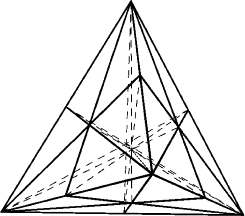
(a) $p=4$

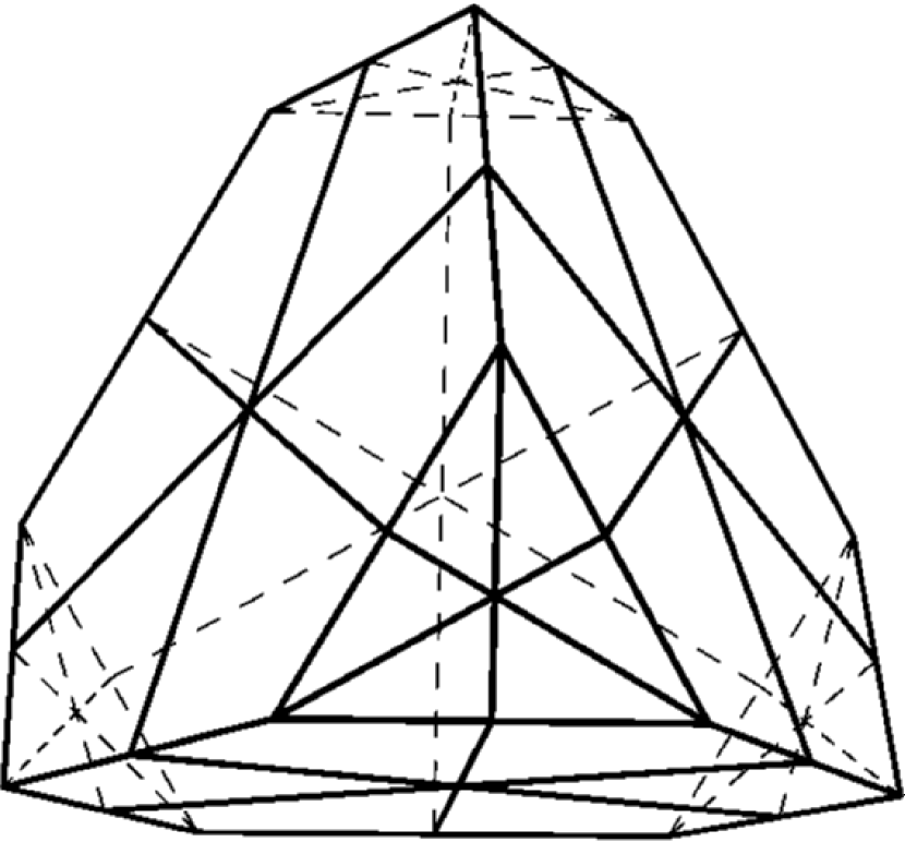
(b) $p=5,6$

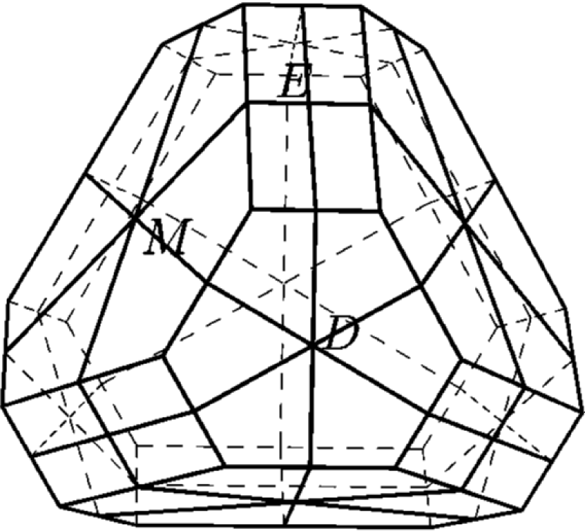
(c)

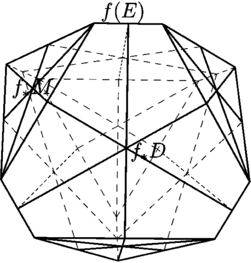
(d) $p=8$

Figure 4. A schematic picture of the process of blowing-up points, then lines, and finally contracting $E$ in the other direction.

The Schwarz condition holds precisely for $p=2,3,4,5,6$ and $8$ (see Figure 7, p. 7 for the values of $\kappa_{L}$ for various strata $L$). For $p=2$ we recover $W(A_{4})$ itself, and for $p=3$ we obtain the Shephard-Todd group $G_{32}$. In particular, the CHL construction applied to the group $G_{32}$ would produce the same list of lattices as the one for $W(A_{4})$ (more precisely, the $G_{32}$ arrangement with constant weight function $1-3/q$ gives the same complex hyperbolic structures as the $A_{4}$ arrangement with constant function $1-2/q$).

For $p=4,5,6$ or $8$, we get lattices in $PU(3,1)$, which we denote by $\mathcal{C}(A_{4},p)$. The volume computation depends on detailed combinatorial properties of the weighted arrangement, and in particular the volume formulas depend on $p$ (see sections 5.1.1 through 5.1.3). What we need from the combinatorics is listed in Figure 7 (on p. 7).

5.1.1. The group $\mathcal{C}(A_{4},4)$

The computation is very easy in this case, since there is no irreducible mirror intersection $L$ with $\kappa_{L}>1$. This means that we do not need any blow-up, i.e. $X=\widehat{X}=Y$, and the orbifold locus is supported by the hyperplane arrangement.

The arrangement has 10 hyperplanes, so the log-canonical divisor is numerically equivalent to $(-4+10(1-\frac{2}{4}))H$, where $H$ denotes the class of a hyperplane, so $(K_{X}+D)^{3}=1$. We have $|\mathbb{P}G|=|G|=120$, and 3-dimensional ball quotients satisfy $c_{1}(X)^{3}=16c_{3}(X)$, so the Euler characteristic is given by

$$-\frac{1}{120\cdot 16}=-\frac{1}{1920}.$$

This is the orbifold Euler characteristic of the Deligne-Mostow lattice for hypergeometric exponents $\mu=(1,1,1,1,1,3)/4$, see Table 3 in [22].

5.1.2. The groups $\mathcal{C}(A_{4},5)$ and $\mathcal{C}(A_{4},6)$

In the case $p=5$, we have $\kappa_{L_{12}}=1-\frac{1}{10}$ and $\kappa_{L_{123}}=1+\frac{1}{5}>1$, so we need to blow up the five points in the $G$ orbit of $\mathbb{P}L_{123}$. Let $\pi:\widehat{X}\rightarrow X$ denote that blow up. A schematic picture of the blow up is given in Figure 4(b) with some inaccuracy in the representation, because the barycenter of the tetrahedron, which is in the same $W(A_{4})$ orbit as the vertices, should be blown-up as well (but this would be too cumbersome to draw).

We denote by $M=M_{1}+\dots+M_{10}$ the proper transform in $\widehat{X}$ of the arrangement. Since there are 6 mirrors through (every element in the $G$-orbit of) $L_{123}$, we have

$$\pi^{*}\pi_{*}M=M+6D,\quad K_{\widehat{X}}=\pi^{*}K_{X}+2D.$$

In the last formula, the factor of $2$ comes from the codimension minus one for the locus blown-up in $\mathbb{P}^{3}$. We then compute, for $\nu,\delta\in\mathbb{Q}$,

$$\left(K_{\widehat{X}}+\nu M+\delta D\right)^{3}$$

$$=\left(\pi^{*}K_{X}+\nu M+(2+\delta)D\right)^{3}$$

$$=\left(\pi^{*}(K_{X}+\nu\pi_{*}M)+\alpha D\right)^{3}$$

$$=\lambda^{3}+5\alpha^{3},$$

where

$$\lambda=-4+10\nu$$

$$\alpha=2+\delta-6\nu.$$

Specializing to $\nu=1-\frac{2}{p}$, $\delta=2-\kappa_{L_{123}}=1-\frac{1}{5}$ (see the tables in section 7), we get $(c_{1}^{orb})^{3}=136/25$, hence

$$\chi^{orb}=c_{3}^{orb}=-\frac{136}{25\cdot 120\cdot 16}=-\frac{17}{6000}.$$

This agrees with the Euler characteristic of the Deligne-Mostow lattice for with $\mu=(3,3,3,3,3,5)/10$.

The same formula also works for $p=6$, where we take $\nu=1-\frac{2}{6}$, $\delta=2-\kappa_{L_{123}}=1-\frac{1}{3}$. In that case, we get

$$\chi^{orb}=-\frac{1}{270}.$$

This is coherent with the formula in [22], note that this lattice has index $6=6!/5!$ in the corresponding Deligne-Mostow lattice, i.e. the one with $\mu=(1,1,1,1,1,1)/3$, and $(-1/270)/6=-1/1620$ (see section 4 for the relationship with Deligne-Mostow lattices).

5.1.3. The group $\mathcal{C}(A_{4},8)$

In this section, we treat the group derived from $A_{4}$ with $p=8$, which corresponds to the Deligne-Mostow group for $\mu=(1,3,3,3,3,3)/8$. Recall that the combinatorics of the arrangement are given in Figure 7 (p. 7), see also Figure 4(a).

The irreducible mirror intersections $L$ with $\kappa_{L}>1$ consist of the 5 lines in the $G$-orbit of $L_{123}$ (in the schematic picture, these correspond to the vertices of the tetrahedron as well as its barycenter), and the 10 two-planes in the $G$-orbit of $L_{12}$ (these correspond to the 6 edges of the tetrahedron, together with its 4 lines joining a vertex to the barycenter). We write $X=\mathbb{P}^{3}$, $\pi_{1}:\widetilde{X}\rightarrow X$ for the blow-up of the five points, $\pi_{2}:\widehat{X}\rightarrow\widetilde{X}$ for the blow-up of the strict transform of the 10 lines through these 5 points, and finally $\pi=\pi_{1}\circ\pi_{2}$. We use the notation from section 5, so that $D$ (resp. $E$) denotes the exceptional divisor in $\widehat{X}$ above points (resp. lines) in $X=\mathbb{P}^{3}$. The space $\widehat{X}$ is depicted in Figure 4(c) (except that we omit drawing the blown-up barycenter and the exceptional divisors above lines incident to the barycenter).

The components of $E$ are copies of $\mathbb{P}^{1}\times\mathbb{P}^{1}$, and the space $Y$ is obtained from $\widehat{X}$ by contracting the fibers of these copies of $\mathbb{P}^{1}\times\mathbb{P}^{1}$ in the other direction than $\pi_{2}$. The resulting space $Y$ is smooth. A schematic picture of $Y$ is drawn in Figure 4(d).

If $f:\widehat{X}\rightarrow Y$ denotes the contraction, the formula (7) gives

$$K_{\widehat{X}}=f^{*}K_{Y}+E.$$

We then use Proposition 1 to each component $E_{j}$, taking $n=2$ in the formulas given there. We first claim that

$$f^{*}f_{*}M=M+E,\qquad f^{*}f_{*}D=D+2E.$$

We explain how to get these formulas from Figure 7, since this is the method we will use for more complicated arrangements, but the reader may also want to glance at Figure 4.

The first formula comes counting the planes in the projectivized arrangement that intersect each given line $\pi(E_{j})$ away from the points blown-up. Indeed, these correspond to the components of $f_{*}M$ that contain $f(E_{j})$.

Recall that $\pi(E_{j})$ is an element in the $G$-orbit of $L_{12}$. The last column (incident vertices) in the $L_{12}$-row of Figure 7 indicates that $L_{12}$ contains three 1-dimensional strata, two in the $G$-orbit of $L_{123}$ and one in the $G$-orbit of $L_{134}$. The first two correspond to points that get blown-up, the third one to a transverse intersection in the $G$-orbit of $L_{1}\cap L_{34}$, which is the same as the $G$-orbit of $L_{4}\cap L_{12}$. This implies that, when pulling-back $f_{*}M$ under $f$, we will pick-up every component $E_{j}$ precisely one, hence the announced formula.

The formula for $f^{*}f_{*}D$ follows from the fact that there are two components of $f_{*}D$ that contain each component $f(E_{k})$ of $f(E)$. Indeed, these correspond to the 1-dimensional mirror intersections $L$ with $\kappa_{L}>1$ that are contained in $\pi(E_{k})$; the number of such 1-dimensional intersections can be found once again in the $L_{12}$ row of Figure 7 (it is indicated by the $2\times L_{123}$ in the column for indicident vertices).

Now we get (for every $\nu,\delta\in\mathbb{Q}$),

$$\left(K_{Y}+\nu f_{*}M+\delta f_{*}D\right)^{3}=$$

$$\left(K_{\widehat{X}}-E+\nu(M+E)+\delta(D+2E)\right)^{3}=$$

$$\left(\pi^{*}K_{X}+2D+E-E+\nu(M+E)+\delta(D+2E)\right)^{3}.$$

Note that

$$\pi^{*}\pi_{*}M=M+6D+3E,$$

since there are six mirrors through each point blown-up (see the third column in the $L_{123}$ row of Figure 7), and three mirrors containing each line blown-up (see the third column in the $L_{12}$ row of Figure 7).

Hence the above formula can be written as

$$\left(\pi^{*}(K_{X}+\nu\pi_{*}M)+(2+\delta-6\nu)D-2(\nu-\delta)E\right)^{3}.$$

We then have

$$(K_{Y}+\Delta)^{3}=\left(\lambda\pi^{*}H+\alpha D+\beta E\right)^{3}$$

where $H$ denotes the class of a plane in $\mathbb{P}^{3}$, and

$$\lambda=-4+10\nu,\quad\alpha=2+\delta-6\nu,\quad\beta=-2(\delta-\nu).$$

Finally, we get

$$(K_{Y}+\Delta)^{3}=$$

$$\lambda^{3}+5\alpha^{3}+10\beta^{3}\cdot E^{3}+3\cdot 10\cdot\beta^{2}(\lambda\pi^{*}H\cdot E^{2}+\alpha D\cdot E^{2})=$$

$$\lambda^{3}+5\alpha^{3}+20\beta^{3}-30\beta^{2}(\lambda+2\alpha).$$

To explain the last two equalities, the key point is that for each irreducible component $E_{j}$ of $E$,

$$E_{j}|_{E_{j}}=-l_{1}-l_{2},$$

where $l_{1}$ and $l_{2}$ are the respective fibers in $\mathbb{P}^{1}\times\mathbb{P}^{1}$.

Note that when developing the cube, most cross-terms disappear because

$$(\pi^{*}H)^{2}\cdot D=(\pi^{*}H)^{2}\cdot E=\pi^{*}H\cdot D^{2}=\pi^{*}H\cdot D\cdot E=0.$$

Indeed, $H$ can be represented by a hyperplane not going through any of the points blown-up, and $H^{2}$ can be represented by a line that does not intersect any of the lines whose strict transform gets blown-up.

Moreover, whenever $D_{k}$ intersects $E_{j}$, $D_{k}|_{E_{j}}=l_{1}$ (see the discussion on p. 1), so $D_{k}^{2}\cdot E_{k}=0$. Also, we can represent $H$ by a plane that is transverse to $\pi(E_{j})$, so that $\pi^{*}H|_{E_{j}}=l_{1}$, so we have

$$D_{k}\cdot E_{j}^{2}=-1,\quad\pi^{*}H\cdot E_{j}^{2}=-1.$$

Finally we have $D_{j}^{3}=1$ and

$$E_{j}^{3}=E_{j}|_{E_{j}}\cdot E_{j}|_{E_{j}}=(-l_{1}-l_{2})^{2}=2,$$

see again the computations on p. 1.

The log-canonical divisor for $\mathcal{C}(A_{4},8)$ is given as above for $\nu=1-\frac{1}{8}$, $\delta=2-\kappa_{L_{123}}=1-\frac{1}{2}$ (see the tables in Figure 8 on p. 8). This gives

$$(K_{Y}+\Delta)^{3}=\frac{33}{8},$$

and finally

$$\chi^{orb}(\mathcal{C}(A_{4},8))=-\frac{11}{5120}.$$

This agrees with the formula in [22].

5.2. The groups derived from the $G_{28}$ arrangement

The combinatorial properties of the $G_{28}$ arrangement are given in the tables of Figure 9, p. 9.

There are two orbits of mirrors of complex reflections in $G=G_{28}$, each containing 12 hyperplanes. The $G$-invariant weight assignments are parametrized by a pair $(p_{1},p_{2})$ of integers.

In fact there is an outer automorphism of $G$ exchanging the two conjugacy classes of complex reflections, so the groups $\mathcal{C}(p_{1},p_{2})$ and $\mathcal{C}(p_{2},p_{1})$ are isomorphic. Without loss of generality, we may and will assume that $p_{1}\leqslant p_{2}$.

The Schwarz condition is of course satisfied for $(p_{1},p_{2})=(2,2)$, in which case the group $\mathcal{C}(G_{28},2,2)$ is simply $G_{28}$. It is also satisfied for $(p_{1},p_{2})=(2,3)$, which gives a parabolic group, i.e. the signature of the invariant Hermitian form is $(3,0)$.

There are 11 other pairs $(p_{1},p_{2})$ with $p_{1}\leqslant p_{2}$ such that where the Schwarz condition holds, listed in the table of Figure 9 (p. 9). We will compute volumes for all cases, grouping them in families where the blow-up $\widehat{X}$ and the contracted space $Y$ have the same description, hence the corresponding volume formulae are similar.

5.2.1. The $G_{28}$ cases where no blow-up is needed

There are two such groups, given by $(p_{1},p_{2})=(2,4)$ or $(3,3)$. As above, we write $\nu_{j}=1-\frac{2}{p_{j}}$. For these two cases we have $\widehat{X}=X=Y$, and $K_{X}+D$ is numerically equivalent to $(-4+12\nu_{1}+12\nu_{2})H$, so

$$(c_{1}^{orb}(\mathbb{B}^{3}/\mathcal{C}(G_{28},p_{1},p_{2}))^{3}=\frac{1}{576}(-4+12\nu_{1}+\nu_{2})^{3},$$

where the denominator 576=1152/2 is the order of the projective group $\mathbb{P}(G_{28})$, in other words $|G_{28}|/|Z(G_{28})|$.

This gives

$$\chi^{orb}((\mathbb{B}^{3}/\mathcal{C}(G_{28},2,4)=-\frac{1}{1152},$$

and

$$\chi^{orb}((\mathbb{B}^{3}/\mathcal{C}(G_{28},3,3)=-\frac{1}{144}.$$

5.2.2. The $G_{28}$ cases where we blow up points

There are 5 pairs of weights where we only blow up points. For $(p_{1},p_{2})=(2,5)$ and $(2,6)$, we blow up the 12 points in the $G$-orbit of $\mathbb{P}L_{234}$. For $(p_{1},p_{2})=(3,4)$, $(3,6)$, $(4,4)$, we blow up two $G$-orbits of points in $X=\mathbb{P}^{3}$, namely the 12 points in the $G$-orbit of $\mathbb{P}L_{234}$ and the 12 points in the $G$-orbit of $\mathbb{P}L_{123}$.

We treat the cases where we blow up two $G$-orbits of points in some detail, the other ones (where we blow-up only one $G$-orbit) are easier. Denote by $\pi:\widehat{X}\rightarrow X$ the corresponding blow up, and by $M_{1}$ and $M_{2}$ the proper transform of the two orbits of mirrors in $G_{28}$.

Write $D_{1}$ (resp. $D_{2}$) for the exceptional divisor above the $G$-orbit of $\mathbb{P}L_{123}$ (resp. $\mathbb{P}L_{234}$). Note that the divisors $D_{j}$ both have 12 disjoint components. We have

$$K_{\widehat{X}}=\pi^{*}K_{X}+2D_{1}+2D_{2}$$

$$\pi^{*}\pi_{*}M_{1}=6D_{1}+3D_{2}$$

$$\pi^{*}\pi_{*}M_{2}=3D_{1}+6D_{2}$$

The last two formulae follow from the count of mirrors of each type through $L_{123}$ (resp. $L_{234}$), see Figure 9 (for $j=1,2$, mirrors of type $j$ are those in the $G$-orbit of the mirror $L_{j}$ of $r_{j}$). Note that $L_{123}$ is on 6 mirrors of type 1 and 3 mirrors of type 2, as is indicated by 6+3 in the third column of the row headed $L_{123}$. Similarly, $L_{234}$ is on 3 mirrors of type 1 and 6 mirrors of type 2.

The relevant divisor for the orbifold pair is

$$\Delta=\nu_{1}M_{1}+\nu_{2}M_{2}+\delta_{1}D_{1}+\delta_{2}D_{2},$$

where, $\nu_{j}=1-\frac{2}{p_{j}}$ and $\delta_{1}=2-\kappa_{L_{123}}$, $\delta_{2}=2-\kappa_{L_{234}}$.

We need to compute

(10) $$(K_{\widehat{X}}+\Delta)^{3}$$

(11) $$=\left(\pi^{*}K_{X}+\nu_{1}M_{1}+\nu_{2}M_{2}+(2+\delta_{1})D_{1}+(2+\delta_{2})D_{2}\right)$$

(12) $$=\left(\lambda\pi^{*}H+\alpha_{1}D_{1}+\alpha_{2}D_{2}\right)^{3}$$

(13) $$=\lambda^{3}+12\alpha_{1}^{3}+12\alpha_{2}^{3}$$

where

$$\lambda=-4+12\nu_{1}+12\nu_{2},\quad\alpha_{1}=2+\delta_{1}-6\nu_{1}-3\nu_{2},\quad\alpha_{2}=2+\delta_{2}-3\nu_{1}-6\nu_{2}.$$

The factors of 12 in equation (13) come from the fact that each $D_{j}$, $j=1,2$ has 12 components, note also that $D_{j}^{3}=1$. When developing the cube, the cross-terms do not contribute since the 24 components of $D_{1}+D_{2}$ are pairwise disjoint, and $H$ can be represented by a plane not containing any of the 24 points blown-up.

Formula (13) gives

$$\chi^{orb}(\mathbb{B}^{3}/\mathcal{C}(G_{28},3,4))=-\frac{23}{1152},$$

$$\chi^{orb}(\mathbb{B}^{3}/\mathcal{C}(G_{28},3,6))=-\frac{1}{36},$$

$$\chi^{orb}(\mathbb{B}^{3}/\mathcal{C}(G_{28},4,4))=-\frac{5}{144}.$$

For the cases $(p_{1},p_{2})=(2,5)$ and $(2,6)$, the formula is the same, except one removes the term corresponding to $D_{1}$ (i.e. the exceptional above the $G$-orbit of $\mathbb{P}L_{123}$, which is not supposed to get blown-up since $\kappa_{L_{123}}<1$). In other words, with the same notation for $\alpha$ and $\lambda$, we have

$$(K_{\widehat{X}}+\Delta)^{3}=\lambda^{3}+12\alpha_{2}^{3}.$$

This gives

$$\chi^{orb}(\mathbb{B}^{3}/\mathcal{C}(G_{28},2,5))=-\frac{13}{4500},$$

$$\chi^{orb}(\mathbb{B}^{3}/\mathcal{C}(G_{28},2,6))=-\frac{5}{1296}.$$

In sections 5.2.3 through 5.2.5, we treat the $G_{28}$ cases where we need to blow up both points and lines.

5.2.3. The case $\mathcal{C}(G_{28},p_{1},p_{2})$ for $(p_{1},p_{2})=(2,8)$ or $(2,12)$

In this case we blow up the 12 points in the $G$-orbit of $\mathbb{P}L_{234}$, and then the strict transform of the 16 lines in the $G$-orbit of $\mathbb{P}L_{34}$. As before, we denote the corresponding composition of blow-ups by $\pi:\widehat{X}\rightarrow X=\mathbb{P}^{3}$ and by $f:\widehat{X}\rightarrow Y$ the relevant contraction, see section 3.

Since each copy of $L_{34}$ contains 3 copies of $L_{234}$, $f:\widehat{X}\rightarrow Y$ is crepant, i.e. $f^{*}K_{Y}=K_{X}$ (see equation (7) for $n=3$).

On $\widehat{X}$ we have $D$ (exceptional divisor with 12 components, above the $G$-orbit of $\mathbb{P}L_{234}$), $E$ (exceptional divisor with 16 components, above the $G$-orbit of $\mathbb{P}L_{34}$), $M_{1}$ and $M_{2}$ (strict transform of the $G$-orbit of mirrors of reflections in $G$, both have 12 components). We will need the following formulae:

$$K_{\widehat{X}}=f^{*}K_{Y}$$

$$f^{*}f_{*}M_{1}=M_{1}+\frac{3}{2}E,\qquad f^{*}f_{*}M_{2}=M_{2}$$

$$f^{*}f_{*}D=D+\frac{3}{2}E$$

$$K_{\widehat{X}}=\pi^{*}K_{X}+2D+E$$

$$\pi^{*}\pi_{*}M_{1}=M_{1}+3D,\qquad\pi^{*}\pi_{*}M_{2}=M_{2}+6D+3E$$

In the formula for $f^{*}f_{*}M_{1}$, the denominator 2 comes from part (2) of Proposition 1, and the numerator 3 comes from the count of the number of components of $f_{*}M_{1}$ that contain the image of a component of $E$ in $Y$. The latter number is given by the number of mirrors in the $G$-orbit of $L_{1}$ that intersect $L_{34}$ transversely, away from the $G$-orbit of $L_{234}$ (these are the points that get blown-up to get $\widehat{X}$). It is indicated by the occurrence of $3\times L_{134}$ in the last column of the row of Figure 9 headed $L_{34}$.

Similarly, in the formula for $f^{*}f_{*}D$, the denominator 2 comes from formula in Proposition 1(3), and the numerator 3 comes from the number of points of $\mathbb{P}L_{34}$ that are in the $G$-orbit of $\mathbb{P}L_{234}$ (see the $3\times L_{234}$ in the row of Figure 9 headed $L_{34}$).

The formulae for $\pi^{*}\pi_{*}M_{j}$ ($j=1,2$) follow from the count of mirrors of each type containing $L_{234}$ (the 3+6 in the table indicates that it is contained in 3 mirrors of type 1, and 6 mirrors of type 2) and $L_{34}$ (0+3 indicates that it is contained in 3 mirrors of type 2).

The same computations as in section 5.1.3 then give

(14) $$\left(K_{X}+\Delta\right)^{3}=\left(\lambda\pi^{*}H+\alpha D+\beta E\right)^{3}$$

where

$$\lambda=-4+12\nu_{1}+12\nu_{2}$$

$$\alpha=2+\delta-3\nu_{1}-6\nu_{2}$$

$$\beta=1+\frac{3}{2}\nu_{1}-3\nu_{2}+\frac{3}{2}\delta$$

and we need to take $\nu_{j}=1-\frac{2}{p_{j}}$, and $\delta=2-\kappa_{L_{234}}$.

When developing the cube in equation (14), most cross-term disappear for the same reason as in section 5.1.3. Once again only terms of the form $D_{k}\cdot{E_{j}}^{2}$ or $\pi^{*}H\cdot{E_{j}}^{2}$ remain, where the $D_{k}$ (resp. $E_{j}$) denotes the $k$-th component of $D$ (resp. the $j$-th component of $E$).

Recall that $E_{j}|_{E_{j}}=-l_{1}-2l_{2}$, where $l_{1}$ is the class in $Pic(E_{j})$ that projects to a line in $\mathbb{P}^{3}$ (see equation (5)). Moreover, $\pi^{*}H$ restricts to $l_{2}$, and $D_{k}$ restricts to either 0 or $l_{2}$ (depending on whether $D_{k}$ and $E_{j}$ intersect at all), see the discussion on p. 1. This gives $\pi^{*}H\cdot E_{j}^{2}=-1$, and $D_{k}\cdot E_{j}^{2}=-1$ (or 0 if $D_{k}$ and $E_{j}$ are disjoint).

Note that $E$ has 16 components, and $\pi^{*}H\cdot E_{j}^{2}=-1$ for each $j$, we have $\pi^{*}H\cdot E^{2}=-16$. Also each component $E_{j}$ of $E$ intersects precisely 3 components of $D$ (see the occurrence of $3\times L_{234}$ in the row for $L_{34}$ of Figure 9), and $D_{k}\cdot E_{j}^{2}=-1$ for each $j$, so $D\cdot E^{2}=-16\cdot 3$.

Finally, we get

$$\lambda^{3}+12\alpha^{3}+16\cdot 4\cdot\beta^{3}-3\cdot 16\cdot\lambda\beta^{2}-3\cdot 16\cdot 3\cdot\alpha\beta^{2}.$$

For $(p_{1},p_{2})=(2,8)$, $\delta=2-\kappa_{L_{234}}=1-\frac{1}{2}$, this gives

$$\chi^{orb}(\mathcal{C}(G_{28},2,8))=-\frac{11}{3072}.$$

For $(p_{1},p_{2})=(2,12)$, $\delta=2-\kappa_{L_{234}}=1-\frac{2}{3}$, this gives

$$\chi^{orb}(\mathcal{C}(G_{28},2,12))=-\frac{23}{10368}.$$

5.2.4. The case $\mathcal{C}(G_{28},6,6)$

In this case we blow up 12 points in the $G$-orbit of $\mathbb{P}L_{123}$, the 12 points in the $G$-orbit of $\mathbb{P}L_{234}$, and then the strict transform of the 18 lines in the $G$-orbit of $\mathbb{P}L_{23}$.

Since each copy of $L_{23}$ contains 2 copies of $L_{234}$ and 2 copies of $L_{123}$ (see the occurrence of $2\times L_{123}$ and $2\times L_{234}$ in the column for “Incident vertices” of the row headed $L_{23}$ in Figure 9), we have

$$K_{\widehat{X}}=f^{*}K_{Y}-\frac{n-3}{n-1}E$$

with $n=2+2=4$, i.e. $f^{*}K_{Y}=K_{\widehat{X}}+\frac{1}{3}E$.

On $\widehat{X}$ we have $D_{1},D_{2},E,M_{1},M_{2}$; here $D_{1}$ (resp. $D_{2}$) is the exceptional divisor above the $G$-orbit of $\mathbb{P}L_{123}$ (resp. $\mathbb{P}L_{234}$). We have the following:

$$K_{\widehat{X}}=f^{*}K_{Y}+\frac{1}{3}E_{1}$$

$$f^{*}f_{*}M_{1}=M_{1},\qquad f^{*}f_{*}M_{2}=M_{2}$$

$$f^{*}f_{*}D_{1}=D_{1}+\frac{2}{3}E,\qquad f^{*}f_{*}D_{2}=D_{2}+\frac{2}{3}E$$

$$K_{\widehat{X}}=\pi^{*}K_{X}+2D_{1}+2D_{2}+E$$

$$\pi^{*}\pi_{*}M_{1}=M_{1}+6D_{1}+3D_{2}+2E,\qquad\pi^{*}\pi_{*}M_{2}=M_{2}+3D_{1}+6D_{2}+2E$$

The claim about $f^{*}f_{*}M_{j}$ follows from the fact that no mirror intersects $L_{23}$ transversely away from the $G$-orbit of $L_{123}$ and away from the $G$-orbit of $L_{234}$.

The claim about $f^{*}f_{*}D_{j}$ follows from Proposition 1(3), and the fact that each $E_{k}$ contains two points of the $G$-orbit of $\mathbb{P}L_{123}$, and two points in the $G$-orbit of $\mathbb{P}L_{234}$.

Computations similar to those in section 5.2.3 now give

$$\left(K_{X}+\Delta\right)^{3}=\left(\lambda\pi^{*}H+\alpha D+\beta E\right)^{3}$$

where

$$\alpha_{1}=2+\delta_{1}-6\nu_{1}-3\nu_{2},\quad\alpha_{2}=2+\delta_{2}-3\nu_{1}-6\nu_{2}$$

$$\lambda=-4+12\nu_{1}+12\nu_{2},\quad\beta=\frac{4}{3}-2\nu_{1}-2\nu_{2}+\frac{2}{3}\delta_{1}+\frac{2}{3}\delta_{2}.$$

In the above formulae, we now take $\nu_{j}=1-\frac{2}{p_{j}}$, $\delta_{1}=2-\kappa_{L_{123}}$, $\delta_{2}=2-\kappa_{L_{234}}$.

Recall that we have $E_{j}^{3}=2\cdot 4-2=6$ for every component $E_{j}$ of $E$, see equation (5). The same analysis of the cross-terms as in section 5.2.3 gives

$$\left(K_{X}+\Delta\right)^{3}=\lambda^{3}+12\alpha_{1}^{3}+12\alpha_{2}^{3}+18\cdot 6\cdot\beta^{3}-3\cdot 18\cdot\lambda\beta^{2}-3\cdot 18\cdot 2\cdot\alpha_{1}\beta^{2}-3\cdot 18\cdot 2\cdot\alpha_{2}\beta^{2}$$

which for $(p_{1},p_{2})=(6,6)$, $\delta_{1}=\delta_{2}=0$ gives

$$\chi^{orb}(\mathcal{C}(G_{28},6,6))=-\frac{5}{144}.$$

5.2.5. The case $\mathcal{C}(G_{28},3,12)$

In this case we blow up the 12 points in the $G$-orbit of $\mathbb{P}L_{123}$, the 12 points in the $G$-orbit of $\mathbb{P}L_{234}$, then the strict transform of the 18 lines in the $G$-orbit of $\mathbb{P}L_{23}$, and the strict transform of the 16 lines in the $G$-orbit of $\mathbb{P}L_{34}$.

On $\widehat{X}$ we now have $D_{1},D_{2},E_{1},E_{2},M_{1},M_{2}$ (where $D_{1}$ corresponds to $L_{123}$, $D_{2}$ to $L_{234}$, $E_{1}$ to $L_{23}$, $E_{2}$ to $L_{34}$).

$$K_{\widehat{X}}=f^{*}K_{Y}-\frac{1}{3}E_{1}$$

$$f^{*}f_{*}M_{1}=M_{1}+\frac{3}{2}E_{2},\qquad f^{*}f_{*}M_{2}=M_{2}$$

$$f^{*}f_{*}D_{1}=D_{1}+\frac{2}{3}E_{1},\qquad f^{*}f_{*}D_{2}=D_{2}+\frac{2}{3}E_{1}+\frac{3}{2}E_{2}$$

$$K_{\widehat{X}}=\pi^{*}K_{X}+2D_{1}+2D_{2}+E_{1}+E_{2}$$

$$\pi^{*}\pi_{*}M_{1}=M_{1}+6D_{1}+3D_{2}+2E_{1},\qquad\pi^{*}\pi_{*}M_{2}=M_{2}+3D_{1}+6D_{2}+2E_{1}+3E_{2}$$

The same computations as before now give

$$\left(K_{X}+\Delta\right)^{3}=\left(\lambda\pi^{*}H+\alpha D+\beta E\right)^{3}$$

where

$$\lambda=-4+12\nu_{1}+12\nu_{2}$$

$$\alpha_{1}=2+\delta_{1}-6\nu_{1}-3\nu_{2},\qquad\alpha_{2}=2+\delta_{2}-3\nu_{1}-6\nu_{2}$$

$$\beta_{1}=\frac{4}{3}-2\nu_{1}-2\nu_{2}+\frac{2}{3}\delta_{1}+\frac{2}{3}\delta_{2},\quad\beta_{2}=1+\frac{3}{2}\nu_{1}-3\nu_{2}+\frac{3}{2}\delta_{1}$$

Developing the cube, we get

$$\lambda^{3}+12\alpha_{1}^{3}+12\alpha_{2}^{3}+18\beta_{1}^{3}\cdot 9+16\beta_{2}^{3}\cdot 4+3\left(\pi^{*}H\cdot E_{1}^{2}+\pi^{*}H\cdot E_{2}^{2}+D_{1}\cdot E_{1}^{2}+D_{2}\cdot E_{1}^{2}+D_{2}\cdot E_{2}^{2}\right)$$

$$=\lambda^{3}+12\alpha_{1}^{3}+12\alpha_{2}^{3}+162\beta_{1}^{3}+64\beta_{2}^{3}-3\left(\cdot 18\cdot\lambda\beta_{1}^{2}+\cdot 16\cdot\lambda\beta_{2}^{2}+\cdot 18\cdot 2\cdot\alpha_{1}\beta_{1}^{2}+\cdot 18\cdot 2\cdot\alpha_{2}\beta_{1}^{2}+\cdot 16\cdot 3\cdot\alpha_{2}\beta_{2}^{2}\right).$$

For $(p_{1},p_{2})=(3,12)$, $\delta_{1}=1-\frac{1}{2}$, $\delta_{2}=1-1=0$, we get

$$\chi^{orb}(\mathcal{C}(G_{28},3,12))=-\frac{23}{1152}.$$

5.3. The groups derived from the $G_{29}$ arrangement

The combinatorial properties of the $G_{29}$ arrangement are given in the tables of Figure 10, p. 10.

Here the group has a single orbit of mirrors of reflections, so the corresponding lattices $\mathcal{C}(G_{29},p)$ are indexed by a single integer $p$. The hyperbolic cases that satisfy the Schwarz condition correspond to $p=3$ or $4$.

The volume computations are similar to the ones in section 5.1.2 or section 5.2.2, since we only blow up points, i.e. in the notation of section 5, $\widehat{X}=Y$.

For $p=3$, we need to blow up the $G$-orbit of $L_{234}$, since $\kappa_{L_{234}}=1+\frac{1}{3}>1$. In this case, we get

$$\left(K_{\widehat{X}}+\Delta\right)^{3}=\lambda^{3}+20\alpha^{3},$$

where

$$\lambda=-4+40\nu$$

$$\alpha=2+\delta-12\nu,$$

where $\nu=1-\frac{2}{p}$ and $\delta=2-\kappa_{234}=1-\frac{1}{3}$. This gives

$$\chi^{orb}(\mathcal{C}(G_{29},3))=-\frac{323}{12960}.$$

For $p=4$, we need to blow up the $G$-orbit of $L_{234}$ (which gives 20 points in $X=\mathbb{P}^{3}$) and the $G$-orbit of $L_{124}$ (which gives 40 points in $X=\mathbb{P}^{3}$), see Figure 10. The formula is similar to the one for $p=3$, we get

$$\left(K_{\widehat{X}}+\Delta\right)^{3}=\lambda^{3}+20\alpha_{1}^{3}+40\alpha_{2}^{3},$$

where

$$\lambda=-4+40\nu$$

$$\alpha_{1}=2+\delta_{1}-12\nu$$

$$\alpha_{2}=2+\delta_{2}-9\nu.$$

Taking $\nu=1-\frac{1}{4}$, $\delta_{1}=2-\kappa_{234}=0$, $\delta_{2}=2-\kappa_{124}=1-\frac{1}{2}$, we get

$$\chi^{orb}(\mathcal{C}(G_{29},4))=-\frac{13}{160}.$$

5.4. The groups derived from the $G_{30}$ arrangement

The combinatorial properties of the $G_{30}$ arrangement are given in the tables of Figure 11, p. 11.

Again, the group has a single orbit of mirrors of reflections. The Schwarz condition holds (and the group is hyperbolic) for $\mathcal{C}(G_{30},p)$, $p=3$ or $5$.

For $p=3$, we only blow up points (given by the 60 points corresponding to the $G$-orbit of $L_{234}$), so the computation is similar to the one in section 5.1.2. We get

$$\left(K_{\widehat{X}}+\Delta\right)^{3}=\lambda^{3}+60\alpha^{3},$$

where

$$\lambda=-4+60\nu$$

$$\alpha=2+\delta-15\nu.$$

Taking $\nu=1-\frac{2}{3}$, $\delta=1-\frac{2}{3}$, we get

$$\chi^{orb}(\mathcal{C}(G_{30},3))=-\frac{52}{2025}.$$

For $p=5$, we blow up 300 points corresponding to the $G$-orbit of $L_{123}$, the 60 points corresponding to the $G$-orbit of $L_{234}$, and then the strict transform of the 72 lines corresponding to the $G$-orbit of $L_{34}$.

We denote the corresponding exceptional divisors by $D_{1},D_{2},E$, and note

$$K_{\widehat{X}}=f^{*}K_{Y}-\frac{1}{2}E$$

$$f^{*}f_{*}L=L+\frac{5}{4}E$$

$$f^{*}f_{*}D_{1}=D_{1},\qquad f^{*}f_{*}D_{2}=D_{2}+\frac{5}{4}E$$

$$K_{\widehat{X}}=\pi^{*}K_{X}+2D_{1}+2D_{2}+E$$

$$\pi^{*}\pi_{*}L=L+6D_{1}+15D_{2}+5E.$$

The same computations as before now give

$$\left(K_{X}+\Delta\right)^{3}=\left(\lambda\pi^{*}H+\alpha_{1}D_{1}+\alpha_{2}D_{2}+\beta E\right)^{3}$$

where

$$\lambda=-4+60\nu$$

$$\alpha_{1}=2+\delta-1-6\nu,\qquad\alpha_{2}=2+\delta_{2}-15\nu$$

$$\beta=\frac{3}{2}-\frac{15}{4}\nu+\frac{5}{4}\delta_{2}.$$

Using the combinatorics and the self intersection of $E_{1}$ and $E_{2}$ (see the previous sections), we get

$$\lambda^{3}+300\alpha_{1}^{3}+60\alpha_{2}^{3}+72\cdot 8\cdot\beta^{3}-3\cdot 72\cdot\lambda\beta^{2}-3\cdot 72\cdot 5\cdot\alpha_{2}\beta^{2}.$$

We then take $\nu=1-\frac{2}{5}$, $\delta_{1}=1-\frac{1}{5}$, $\delta_{2}=1-2=-1$, and get

$$\chi^{orb}(\mathcal{C}(G_{30},5))=-\frac{41}{1125}.$$

5.5. The groups derived from the $G_{31}$ arrangement

The combinatorial properties of the $G_{31}$ arrangement are given in the tables of Figure 12, p 12.

There are two values of $p$ such that the Schwarz condition and the group $\mathcal{C}(G_{31},p)$ is hyperbolic, namely $p=3$ or $p=5$.

For $p=3$, we need to blow up the 60 points corresponding to the $G$-orbit of $L_{125}$. We get

$$\left(K_{\widehat{X}}+\Delta\right)^{3}=\lambda^{3}+60\alpha^{3},$$

where

$$\lambda=-4+60\nu$$

$$\alpha=2+\delta-15\nu.$$

Taking $\nu=1-\frac{2}{3}$, $\delta=1-\frac{2}{3}$, we get

$$\chi^{orb}(\mathcal{C}(G_{31},3))=-\frac{13}{810}.$$

For $p=5$, we blow up the 60 points corresponding to the $G$-orbit of $L_{125}$, the 480 points corresponding to the $G$-orbit of $L_{235}$, and then the 30 lines corresponding to the $G$-orbit of $L_{14}$.

We denote the corresponding exceptionals by $D_{1},D_{2},E$, and note

$$K_{\widehat{X}}=f^{*}K_{Y}-\frac{3}{5}E$$

$$f^{*}f_{*}L=L$$

$$f^{*}f_{*}D_{1}=D_{1}+\frac{6}{5}E,\qquad f^{*}f_{*}D_{2}=D_{2}$$

$$K_{\widehat{X}}=\pi^{*}K_{X}+2D_{1}+2D_{2}+E$$

$$\pi^{*}\pi_{*}L=L+15D_{1}+6D_{2}+6E.$$

The same computations as before now give

$$\left(K_{X}+\Delta\right)^{3}=\left(\lambda\pi^{*}H+\alpha_{1}D_{1}+\alpha_{2}D_{2}+\beta E\right)^{3}$$

where

$$\lambda=-4+60\nu$$

$$\alpha_{1}=2+\delta_{1}-15\nu$$

$$\alpha_{2}=2+\delta_{2}-6\nu$$

$$\beta=\frac{8}{5}-6\nu+\frac{6}{5}\delta_{2}.$$

Using the combinatorics and the self intersection of $E_{1}$ and $E_{2}$ (see the previous sections), we get

$$\lambda^{3}+60\alpha_{1}^{3}+480\alpha_{2}^{3}+30\cdot 10\cdot\beta^{3}-3\cdot 30\cdot\lambda\beta^{2}-3\cdot 30\cdot 6\cdot\alpha_{1}\beta^{2}.$$

Finally, taking $\nu=1-\frac{2}{5}$, $\delta_{1}=-1$, $\delta_{2}=1-\frac{1}{5}$, we get

$$\chi^{orb}(\mathcal{C}(G_{31},5))=-\frac{41}{1125}.$$

5.6. The groups derived from the $B_{4}$ arrangement

For completeness, we compute the volumes of the CHL groups associated to the $B_{4}$ arrangement, even though the corresponding volumes are known. Indeed, the lattices of the form $\mathcal{C}(B_{4},p_{1},p_{2})$ are commensurable to certain Deligne-Mostow groups (see section 4).

The combinatorial properties of the $B_{4}$ arrangement are given in the tables of Figure 8, p. 8. In this case, the group $G=W(B_{4})$ has two orbits of mirrors of complex reflections. In the numbering used in Figure 8, the mirror of $r_{1}$ is not in the same orbit as the mirror of $r_{2}$ (but the mirror of $r_{3}$ is in the same orbit as the mirror of $r_{2}$, since the braid relation $r_{2}r_{3}r_{2}=r_{3}r_{2}r_{3}$ implies that $r_{2}$ and $r_{3}$ are conjugate in $W(B_{4})$, since $r_{3}=r_{2}r_{3}\cdot r_{2}\cdot(r_{2}r_{3})^{-1}$).

The $G$-invariant weight assignments are determined by the two weights $\kappa_{1}=1-\frac{2}{p_{1}}$ and $\kappa_{2}=1-\frac{2}{p_{2}}$, where $p_{j}$ are integers $\geq 2$. As before, we denote by $\mathcal{C}(B_{4},p_{1},p_{2})$ the corresponding group.

For $(p_{1},p_{2})=(n,2)$ for some $n\geq 2$, the group $\mathcal{C}(B_{4},p_{1},p_{2})$ turns out to be finite (in the Shephard-Todd notation, it is given by the group $G(n,1,4)$, which is imprimitive for $n>2$). For $(p_{1},p_{2})=(2,3)$, the Hermitian form preserved by the group is degenerate of signature (3,0), and the corresponding group gives a complex affine crystallographic group acting on $\mathbb{C}^{3}$ (see section 5 of [9]).

The other pairs $(p_{1},p_{2})$ where the Schwarz condition holds are all hyperbolic (i.e. the group $\mathcal{C}(B_{4},p_{1},p_{2})$ preserves a Hermitian form of signature $(3,1)$). The list of these pairs is given in Figure 8. We treat them separately over sections 5.6.1–5.6.7, according to the dimension of the strata of the arrangement that need to be blown-up in order to describe the quotient $\mathbb{B}^{3}/\mathcal{C}(B_{4},p_{1},p_{2})$.

5.6.1. The groups $\mathcal{C}(B_{4},2,4)$ and $\mathcal{C}(B_{4},3,3)$

In these cases, no blow-up is needed, since $\kappa_{L}\leq 1$ for every irreducible mirror intersection in the arrangement. In other words, in the notation of section 5, we have $X=\widehat{X}=Y$. Since there are 4 mirrors in the first orbit and 12 mirrors in the second orbit, the log-canonical divisor is given on the level of $\mathbb{P}^{3}$ by $(-4+4\nu_{1}+12\nu_{2})H$, where $\nu_{j}=1-\frac{2}{p_{j}}$ and $H$ denotes the hyperplane class.

Up to removal of the cusp, the ball quotient is given by $X/G$ where $G=W(B_{4})$ (with a different orbifold structure than the one coming from this finite quotient), so we have

$$c_{1}^{orb}(\mathbb{B}^{3}/\mathcal{C}(B_{4},p_{1},p_{2}))=\frac{1}{|\mathbb{P}(G)|}(K_{X}+\Delta)^{3}=\frac{1}{192}\left(-4+4\nu_{1}+12\nu_{2}\right)^{3},$$

which gives

$$\chi^{orb}(\mathbb{B}^{3}/\mathcal{C}(B_{4},p_{1},p_{2}))=-\frac{1}{16\cdot 192}\left(-4+4\nu_{1}+12\nu_{2}\right)^{3}.$$

For $(p_{1},p_{2})=(3,3)$, we get $-1/1296$ , which is the orbifold Euler characteristic of $\Gamma_{\mu,\Sigma}$ for hypergeometric exponents $\mu=(1,1,1,1,3,5)/6$, $\Sigma\simeq S_{4}$ (see [22]).

For $(p_{1},p_{2})=(2,4)$, we get $-1/384$, which is the Euler characteristic of $\Gamma_{\mu,\Sigma_{0}}$ for $\mu=(1,1,1,1,1,3)/4$ and $\Sigma_{0}\subset\Sigma\simeq S_{5}$ fixing one of the 5 equal weights. This is coherent with the value given in [22], which is $-1/1920$, since $\Gamma_{\mu,\Sigma_{0}}$ has index 5 in $\Gamma_{\mu,\Sigma}$.

5.6.2. The groups $\mathcal{C}(B_{4},p_{1},p_{2})$ for $(p_{1},p_{2})=(3,4)$, $(4,3)$, $(4,4)$ and $(6,3)$

In these cases, there is a single $G$-orbit of irreducible mirror intersections $L$ with $\kappa_{L}>1$, namely the $G$-orbit of $L_{123}$ (see Table 8). We then have $Y=\widehat{X}$, where $X$ is obtained from $X=\mathbb{P}^{3}$ by blowing up the $G$-orbit of $L=L_{123}$, which gives 4 points in $\mathbb{P}^{3}$. The relevant log-canonical divisor has the form

$$K_{\widehat{X}}+\nu_{1}M_{1}+\nu_{2}M_{2}+\delta D,$$

where $\nu_{j}=1-\frac{2}{p_{j}}$ and $\delta=2-\kappa_{L}$.

Note that $M_{1}$ has 4 components, whereas $M_{2}$ has 12, see Figure 8 on p. 8. Note also that $K_{\widehat{X}}=\pi^{*}K_{X}+2D$, and

$$\pi^{*}\pi_{*}M_{1}=M_{1}+3D,\quad\pi^{*}\pi_{*}M_{2}=M_{2}+6D,$$

since $L_{123}$ is on 3 mirrors in the first orbit, and 6 mirrors in the second orbit.

Now the log-canonical divisor can be rewritten as

$$\pi^{*}(K_{X}+A)+\alpha D,$$

where $A=K_{X}+\nu_{1}M_{1}+\nu_{2}M_{2}$ and

$$\alpha=2+\delta-3\nu_{1}-6\nu_{2}.$$

Finally, observe that $K_{X}+A$ is linearly equivalent to $\lambda H$ where

$$\lambda=-4+4\nu_{1}+12\nu_{2},$$

and we get

$$(c_{1}(\widehat{X},\mathcal{D}))^{3}=\lambda^{3}+4\alpha^{3}.$$

Indeed, $D$ has 4 components (corresponding to the fact that the $G$-orbit of $L_{123}$ has 4 points), and for each component $D_{j}$, we have $D_{j}^{3}=1$.

For $(p_{1},p_{2})=(3,4)$, we get

$$\chi^{orb}(\mathbb{B}^{3}/\mathcal{C}(B_{4},3,4))=-\frac{31}{3456}.$$

This is the same as the value of the orbifold Euler characteristic of the Deligne-Mostow group $\Gamma_{\mu,\Sigma}$ for $\mu=(3,3,3,3,5,7)/12$, $\Sigma=S_{4}$ (note that this is actually the non-arithmetic lattice in $PU(3,1)$ constructed by Deligne and Mostow).

For $(p_{1},p_{2})=(3,4)$, we get

$$\chi^{orb}(\mathbb{B}^{3}/\mathcal{C}(B_{4},4,3))=-\frac{23}{10368}.$$

This is the same as the value of the orbifold Euler characteristic of the Deligne-Mostow group $\Gamma_{\mu,\Sigma}$ for $\mu=(2,2,2,2,7,9)/12$, $\Sigma=S_{4}$.

For $(p_{1},p_{2})=(4,4)$, we get

$$\chi^{orb}(\mathbb{B}^{3}/\mathcal{C}(B_{4},4,4))=-\frac{1}{96}.$$

This is the same as the value of the orbifold Euler characteristic of the Deligne-Mostow group $\Gamma_{\mu,\Sigma_{0}}$ for $\mu=(1,1,1,1,2,2)/4$, $\Sigma_{0}=S_{4}$ (the maximal Deligne-Mostow lattice for these weights corresponds to $\Sigma=S_{4}\times S_{2}$, and it has orbifold Euler characteristic $-1/192$).

For $(p_{1},p_{2})=(6,3)$, we get

$$\chi^{orb}(\mathbb{B}^{3}/\mathcal{C}(B_{4},6,3))=-\frac{1}{324}.$$

This is the same as the value of the orbifold Euler characteristic of the Deligne-Mostow group $\Gamma_{\mu,\Sigma_{0}}$ for $\mu=(1,1,1,1,4,4)/6$, $\Sigma_{0}=S_{4}$ (again, the maximal Deligne-Mostow lattice for these weights corresponds to $\Sigma=S_{4}\times S_{2}$, so its Euler characteristic is $-1/648$).

5.6.3. The groups $\mathcal{C}(B_{4},p_{1},p_{2})$ for $(p_{1},p_{2})=(2,5)$, $(2,6)$ and $(3,6)$

This case is similar to the previous one, except that now we need to blow up the 4 points in the $G$-orbit of $L_{123}$, as well as the 8 points in the $G$-orbit of $L_{234}$.

The relevant log-canonical divisor has the form

$$K_{\widehat{X}}+\nu_{1}M_{1}+\nu_{2}M_{2}+\delta_{1}D_{1}+\delta_{2}D_{2}.$$

where $\nu_{j}=1-\frac{2}{p_{j}}$, and $\delta_{1}=2-\kappa_{L{123}}$, $\delta_{2}=2-\kappa_{L{234}}$. Here we denote by $D_{1}$ (resp. $D_{2}$) the exceptional divisors above the $G$-orbit of the projectivization of $L_{123}$ (resp. $L_{234}$).

Note that $M_{1}$ has 4 components, whereas $M_{2}$ has 12, see Figure 8. Note also that $K_{\widehat{X}}=\pi^{*}K_{X}+2D_{1}+2D_{2}$, and

$$\pi^{*}\pi_{*}M_{1}=M_{1}+3D_{1},\quad\pi^{*}\pi_{*}M_{2}=M_{2}+6D_{1}+6D_{2}.$$

Indeed, each element in the orbit of $L_{123}$ lies on 3 components of $M_{1}$ and 6 components of $M_{2}$, and each element in the orbit of $L_{234}$ lies on (no component of $M_{1}$ and) 6 components of $M_{2}$.

We get

$$(K_{\widehat{X}}+\Delta)^{3}=(-4+4\nu_{1}+12\nu_{2})^{3}+4(2+\delta-3\nu_{1})^{3}+8(2+\delta_{2}-6\nu_{1}-6\nu_{2})^{3}.$$

For $(p_{1},p_{2})=(2,5)$, we take $\nu_{j}=1-2/p_{j}$, $\delta_{1}=\delta_{2}=1-1/5$ (see the tables in Figure 8), we get

$$(c_{1}^{orb})^{3}=-\frac{1}{192}(K_{\widehat{X}}+\Delta)^{3}=-\frac{52}{375},$$

so

$$\chi^{orb}(\mathbb{B}^{3}/\mathcal{C}(B_{4},2,5))=-\frac{13}{1500}.$$

This agrees with the Euler characteristic of the Deligne-Mostow lattice $\Gamma_{\mu,\Sigma}$ with $\mu=(2,3,3,3,3,6)/10$, $\Sigma=S_{4}$.

For $(p_{1},p_{2})=(2,6)$, we take $\delta_{1}=\delta_{2}=1-1/3$ and get

$$\chi^{orb}((\mathbb{B}^{3}/\mathcal{C}(B_{4},2,6)))=-\frac{5}{432}.$$

This agrees with the Euler characteristic of the Deligne-Mostow lattice $\Gamma_{\mu,\Sigma}$ with $\mu=(1,2,2,2,2,3)/6$, $\Sigma=S_{4}$.

For $(p_{1},p_{2})=(3,6)$, we take $\delta_{1}=\delta_{2}=1-1/3$ and get

$$\chi^{orb}((\mathbb{B}^{3}/\mathcal{C}(B_{4},3,6)))=-\frac{5}{432}.$$

This agrees with the Euler characteristic of the Deligne-Mostow lattice $\Gamma_{\mu,\Sigma_{0}}$ with $\mu=(1,1,1,1,1,1)/6$, $\Sigma_{0}=S_{4}$. Note that this has index $30=6!/4!$ in the lattice $\Gamma_{\mu,\Sigma}$ with $\Sigma=S_{6}$.

5.6.4. The cases $\mathcal{C}(B_{4},(p_{1},p_{2}))$ with $(p_{1},p_{2})=(6,4)$ or $(12,3)$

Here there are both lines and planes among the mirror intersections $L$ that satisfy $\kappa_{L}>1$, which correspond to the $G$-orbit of $L_{123}$ (this gives 4 points in $\mathbb{P}^{3}$) and the $G$-orbit of $L_{12}$ (this gives 6 lines in $\mathbb{P}^{3}$).

We denote by $M_{1}$ and $M_{2}$ the strict tranform in $\widehat{X}$ of the two $G$-orbits of mirrors ($M_{1}$ has 4 components, whereas $M_{2}$ has 12). We denote by $D$ (resp. $E$) the exceptional divisor in $\widehat{X}$ above the $G$-orbit of $L_{123}$ (resp. the $G$-orbit of $L_{12}$).

We need to compute

$$\left(K_{Y}+\nu_{1}f_{*}M_{1}+\nu_{2}f_{*}M_{2}+\delta f_{*}D\right)^{3},$$

where $\nu_{j}=1-\frac{2}{p_{2}}$ and $\delta=2-\kappa_{L_{123}}$.

We have $K_{\widehat{X}}=f^{*}K_{Y}+E$ (see equation (7)), and one checks using the combinatorics of the arrangement that

$$f^{*}f_{*}M_{1}=M_{1},\quad f^{*}f_{*}M_{2}=M_{2}+2E,\quad f^{*}f_{*}D=D+2E.$$

Note also that

$$\pi^{*}\pi_{*}M_{1}=M_{1}+3D+2E,\quad\pi^{*}\pi_{*}M_{2}=M_{2}+6D+2E,$$

because for each $j$, $\pi_{*}D_{j}$ is on 3 mirrors in the first orbit, and 6 mirrors in the second orbit, and $\pi^{*}E_{j}$ lies on 2 mirrors from each orbit.

This gives

$$(K_{Y}+\Delta)^{3}=\left(\lambda\pi^{*}H+\alpha D+\beta E\right)^{3}$$

where

$$\lambda=-4+4\nu_{1}+12\nu_{2},\quad\alpha=2+\delta-3\nu_{1}-6\nu_{2},\quad\beta=2(\delta-\nu_{1}).$$

Finally we get

$$(K_{Y}+\Delta)^{3}=\lambda^{3}+4\alpha^{3}+6\beta^{3}\cdot 2+3\lambda\beta^{2}\pi^{*}H\cdot E^{2}+3\alpha\beta^{2}D\cdot E^{2}$$

$$=\lambda^{3}+4\alpha^{3}+6\beta^{3}\cdot 2-3\cdot 6\cdot\lambda\beta^{2}-3\cdot 6\cdot 2\cdot\alpha\beta^{2}.$$

For $p_{1}=6$, $p_{2}=4$, we take $\nu_{j}=1-\frac{2}{p_{j}}$ and $\delta=1-\frac{2}{3}$, this gives

$$\chi^{orb}(\mathcal{C}(B_{4},6,4))=-\frac{31}{3456},$$

and for $p_{1}=12$, $p_{2}=3$, we take $\nu_{j}=1-\frac{2}{p_{j}}$ and $\delta=1-\frac{1}{2}$, this gives

$$\chi^{orb}(\mathcal{C}(B_{4},12,3))=-\frac{23}{10368},$$

as it should in comparison with the values expected from [22].

5.6.5. The cases $\mathcal{C}(B_{4},(p_{1},p_{2}))$ with $(p_{1},p_{2})=(6,6)$ or $(10,5)$

Here the situation is almost the same as in section 5.6.4. In order to get $\widehat{X}$, we need to blow up the image in $\mathbb{P}^{3}$ of the $G$-orbit of $L_{123}$ and the $G$-orbit of $L_{234}$, then blow up the strict transform of the $G$-orbit of $L_{12}$.

The incidence data in Figure 8 indicates that $L_{12}$ does not contain any point in the $G$-orbit of $L_{234}$. Indeed, each 2-plane in the $G$-orbit of $L_{12}$ contains precisely 4 one-dimensional mirror intersections, two in the $G$-orbit of $L_{123}$ and two in the $G$-orbit of $L_{124}$.

In other words, one gets the same formula as in section 5.6.4 with $D$ replaced by $D_{1}$ and $D_{2}$, but $D_{2}$ has no interaction with either $D_{1}$ or $E$. With the notation

$$\lambda=-4+4\nu_{1}+12\nu_{2}$$

$$\alpha_{1}=2+\delta_{1}-3\nu_{1}-6\nu_{2},\qquad\alpha_{2}=2+\delta_{2}-6\nu_{2}$$

$$\beta=2(\delta_{1}-\nu_{1}),$$

this gives

$$(K_{Y}+\Delta)^{3}=\lambda^{3}+4\alpha_{1}^{3}+8\alpha_{2}^{3}+6\beta^{3}\cdot 2-3\cdot 6\cdot\lambda\beta^{2}-3\cdot 6\cdot 2\cdot\alpha_{1}\beta^{2},$$

For $p_{1}=6$, $p_{2}=6$, we take $\nu_{j}=1-\frac{2}{p_{j}}$ and $\delta_{1}=2-\kappa_{L{123}}=0$, $\delta_{2}=2-\kappa_{L_{234}}=1-\frac{1}{3}$ (see the Table in Figure 8), which gives $m_{1}=1$, $m_{2}=3$, we get

$$\chi^{orb}(\mathcal{C}(B_{4},6,6))=-\frac{5}{432},$$

and for $p_{1}=10$, $p_{2}=5$, $\delta_{1}=2-\kappa_{L{123}}=0$, $\delta_{2}=2-\kappa_{L_{234}}=1-\frac{1}{5}$ we get

$$\chi^{orb}(\mathcal{C}(B_{4},10,5))=-\frac{13}{1500},$$

as expected.

5.6.6. The case $\mathcal{C}(B_{4}(2,8))$

This case is similar to the previous one. We now wish to compute

$$\left(K_{Y}+\nu_{1}f_{*}M_{1}+\nu_{2}f_{*}M_{2}+\delta_{1}D_{1}+\delta_{2}D_{2}\right)^{3},$$

where $\nu_{j}=1-\frac{2}{p_{j}}$, $\delta_{1}=2-\kappa_{L_{123}}$, $\delta_{2}=2-\kappa_{L_{234}}$. Note that

$$K_{\widehat{X}}=K_{Y}$$

$$f^{*}f_{*}M_{1}=M_{1}+\frac{1}{2}E,\qquad f^{*}f_{*}M_{2}=M_{2}$$

$$f^{*}f_{*}D_{1}=D_{1}+\frac{1}{2}E,\qquad f^{*}f_{*}D_{2}=D_{2}+E.$$

Indeed, each line in $\mathbb{P}^{3}$ below a component of $E$ contains three of the points that get blown-up (one in the orbit of $L_{123}$, two in the orbit of $L_{234}$), and it has a single transverse intersection with a mirror in the first orbit of mirrors.

Using the blow-up map and the combinatorics of the arrangement, we have

$$\pi^{*}\pi_{*}M_{1}=M_{1}+3D_{1}$$

$$\pi^{*}\pi_{*}M_{2}=M_{2}+6D_{1}+6D_{2}+3E,$$

and computations similar to the ones in the previous sections show that $(K_{Y}+\Delta)^{3}$ is given by

$$\left(\lambda\pi^{*}H+\alpha_{1}D_{1}+\alpha_{2}D_{2}+\beta E\right)^{3}$$

where

$$\lambda=-4+4\nu_{1}+12\nu_{2}$$

$$\alpha_{1}=2+\delta_{1}-3\nu_{1}-6\nu_{2},\qquad\alpha_{2}=2+\delta_{2}-6\nu_{2}$$

$$\beta=1+\frac{1}{2}\nu_{1}-3\nu_{2}+\frac{1}{2}\delta_{1}+\delta_{2}.$$

Finally, developing the cube, we get

$$\lambda^{3}+4\alpha_{1}^{3}+8\alpha_{2}^{3}+16\beta^{4}\cdot 4+3\alpha_{1}\beta^{2}D_{1}\cdot E^{2}+3\alpha_{2}\beta^{2}D_{2}\cdot E^{2}+3\lambda\beta^{2}\pi^{*}H\cdot E^{2}.$$

Using the combinatorics and the above description for $E_{j}|_{E_{j}}$ (see equation (5)), we get

$$\lambda^{3}+4\alpha_{1}^{3}+8\alpha_{2}^{3}+16\beta^{4}\cdot 4-3\cdot 16\cdot\alpha_{1}\beta^{2}-3\cdot 16\cdot 2\cdot\alpha_{2}\beta^{2}-3\cdot 16\cdot\lambda\beta^{2}.$$

This gives

$$\chi^{orb}(\mathcal{C}(B_{4},2,8))=-\frac{11}{1024}=-\frac{11}{5120}\cdot 5,$$

as it should since is has index 5 in the corresponding Deligne-Mostow group (see Figure 1).

5.6.7. The case $\mathcal{C}(B_{4}(4,8))$

This case is the most painful case to handle, but it simply combines the difficulties we have encountered before. Here we blow up the orbits of $L_{123}$ (4 copies), $L_{234}$ (8 copies), $L_{12}$ (6 copies) and $L_{23}$ (16 copies). Accordingly we have 4 exceptionals $D_{1},D_{2},E_{1},E_{2}$ in $\widehat{X}$, and still wish to compute

$$\left(K_{Y}+\nu_{1}f_{*}M_{1}+\nu_{2}f_{*}M_{2}+\delta_{1}D_{1}+\delta_{2}D_{2}\right)^{3},$$

again with $\nu_{j}=1-\frac{2}{p_{j}}$, $\delta_{1}=2-\kappa_{L_{123}}$, $\delta_{2}=2-\kappa_{L_{234}}$. Note that

$$K_{\widehat{X}}=f^{*}K_{Y}+E_{1}$$

$$f^{*}f_{*}M_{1}=M_{1}+\frac{1}{2}E_{2},\qquad f^{*}f_{*}M_{2}=M_{2}+2E_{1}$$

$$f^{*}f_{*}D_{1}=D_{1}+2E_{1}+\frac{1}{2}E_{2},\qquad f^{*}f_{*}D_{2}=D_{2}+E_{2}$$

$$K_{\widehat{X}}=\pi^{*}K_{X}+2D_{1}+2D_{2}+E_{1}+E_{2}$$

$$\pi^{*}\pi_{*}M_{1}=M_{1}+3D_{1}+2E_{1},\qquad\pi^{*}\pi_{*}M_{2}=M_{2}+6D_{1}+6D_{2}+2E_{1}+3E_{2}$$

The same computations as before now give

$$\left(K_{X}+\Delta\right)^{3}=\left(\lambda\pi^{*}H+\alpha_{1}D_{1}+\alpha_{2}D_{2}+\beta_{1}E_{1}+\beta_{2}E_{2}\right)^{3}$$

where

$$\lambda=-4+4\nu_{1}+12\nu_{2}$$

$$\alpha_{1}=2+\delta_{1}-3\nu_{1}-6\nu_{2},\qquad\alpha_{2}=2+\delta_{2}-6\nu_{2}$$

$$\beta_{1}=2(\delta_{1}-\nu_{2}),\qquad\beta_{2}=1+\frac{1}{2}\nu_{1}-3\nu_{2}+\frac{1}{2}\delta_{1}+\delta_{2}.$$

Inspecting the combinatorics of the arrangement and using $E_{1}^{(j)}|_{E_{1}^{(j)}}=-l_{1}-2l_{2}$, $E_{2}^{(j)}|_{E_{2}^{(j)}}=-l_{1}-l_{2}$, we then get

$$\lambda^{3}+4\alpha_{1}^{3}+8\alpha_{2}^{3}+16\cdot 4\cdot\beta_{1}^{3}+6\cdot 2\cdot\beta_{2}^{3}-3\cdot 6\lambda\beta_{1}^{2}-3\cdot 16\lambda\beta_{2}^{2}-3\cdot 6\cdot 2\alpha_{1}\beta_{1}^{2}-3\cdot 16\alpha_{1}\beta_{2}^{2}-3\cdot 16\cdot 2\alpha_{2}\beta_{2}^{2}.$$

This gives

$$\chi^{orb}(\mathcal{C}(B_{4},4,8))=-\frac{11}{1024},$$

which is again the expected value.

6. Presentations

From the above results, one can easily obtain explicit presentations for the CHL lattices. Indeed, recall that we denote $V=\mathbb{C}^{n+1}$, $V^{0}\subset V$ the complement of the arrangement (given by the union of the mirrors of reflections in $G$). According to Theorem 7.1 in [9], a presentation for the linear holonomy group is given by adjoining to a presentation of the braid group $\pi_{1}(G\backslash V^{0})$ some specific relations corresponding to the (irreducible) strata in the arrangement. More specifically, for each irreducible stratum $L$, consider the set of mirrors $\mathcal{H}_{L}$ that contain $L$, and the braid group $G_{L}$ generated by the reflections in the elements in $\mathcal{H}_{L}$, which has infinite cyclic center, generated by an element $\alpha_{L}$. If $\rho:\pi_{1}(G\backslash V^{0})\rightarrow\Gamma$ denotes the holonomy representation, the CHL relations correspond to imposing the order of $\rho(\alpha_{L})$, given by the integer that occurs in the Schwarz condition (3). In fact, among those relations, only the ones where the mirror intersection $L$ of dimension or codimension one are needed, since these are the such that the fixed point set of the local holonomy group has fixed point set of codimension one (and these are enough to present the orbifold fundamental group).

Presentations $\pi_{1}(\mathbb{P}(V^{0}/G))$ are given in [3] (some of the results given there were conjectural at the time, but the proof of their validity was given by Bessis in [2]). It is easy to determine conjugacy classes of loops corresponding to the conjugacy classes described in section 7.1 of [9], by determining the conjugacy classes of (irreducible) mirror intersections in $G$, and then taking a generator of the center of each stabilizer.

The corresponding central elements are listed in Tables 1–5 in [6], for instance. One can also check their result by using the explicit matrices described in [11]. For example, we list $(R_{1}R_{2}R_{3})^{3}$ which generates the center of the braid group generated by $R_{1}$, $R_{2}$ and $R_{3}$. Indeed, these generate a braid group of type $G_{26}$, and a generator for the center is given in the fifth column of Table 1 in [6].

We list the relevant central elements in Table 5; these give complex reflections in the lattice, whose order is the integer occurring in the Schwarz condition for $L$, and the relation is needed in the presentation only if $\kappa_{L}>1$. For example, in the groups $\mathcal{C}(A_{4},p)$, $M=(R_{1}R_{2}R_{3})^{4}$ is a complex reflection of order $(\kappa_{L_{123}}-1)^{-1}=\frac{p}{p-4}$, and this relation is needed in the presentation only for $p=5,6$ or $8$.

$A_{4}$	$(R_{1}R_{2}R_{3})^{4}$
$B_{4}$	$(R_{1}R_{2}R_{3})^{3}$, $(R_{2}R_{3}R_{4})^{4}$
$G_{28}$	$(R_{1}R_{2}R_{3})^{3}$, $(R_{2}R_{3}R_{4})^{3}$
$G_{29}$	$(R_{1}R_{2}R_{3})^{4}$, $(R_{1}R_{2}R_{4})^{3}$, $(R_{4}R_{3}R_{2})^{8}$, $(R_{1}R_{2}R_{3}^{-1}R_{4}R_{3})^{4}$
$G_{30}$	$(R_{1}R_{2}R_{3})^{4}$, $(R_{2}R_{3}R_{4})^{5}$
$G_{31}$	$(R_{5}R_{2}R_{1})^{\frac{4p}{p\wedge 3}}$, $(R_{2}R_{3}R_{5})^{4}$

Figure 5. Complex reflections corresponding to central elements in $G_{L}$ for irreducible mirror intersection of dimension one.

Collecting all this, we get the presentations in Figure 6 (p. 6).

Presentation for $\mathcal{C}(A_{4},p)$:

$$\langle\quad r_{1},r_{2},r_{3},r_{4} | r_{1}^{p},(r_{1}r_{2}r_{3})^{\frac{4p}{p-4}},$$

$${\rm br}_{3}(r_{1},r_{2}),{\rm br}_{3}(r_{2},r_{3}),{\rm br}_{3}(r_{3},r_{4}),[r_{1},r_{3}],[r_{1},r_{4}],[r_{2},r_{4}]\quad\rangle$$

 
Presentation for $\mathcal{C}(B_{4},p_{1},p_{2})$:

$$\langle\quad r_{1},r_{2},r_{3},r_{4} | r_{1}^{p_{1}},r_{2}^{p_{2}},(r_{1}r_{2}r_{3})^{\frac{3p_{1}p_{2}}{p_{1}p_{2}-2p_{1}-p_{2}}},(r_{2}r_{3}r_{4})^{\frac{4p_{2}}{p_{2}-4}},$$

$${\rm br}_{3}(r_{1},r_{2}),{\rm br}_{3}(r_{2},r_{3}),{\rm br}_{3}(r_{3},r_{4}),[r_{1},r_{3}],[r_{1},r_{4}],[r_{2},r_{4}]\quad\rangle$$

 
Presentation for $\mathcal{C}(G_{28},p_{1},p_{2})$:

$$\langle\quad r_{1},r_{2},r_{3},r_{4} | r_{1}^{p_{1}},r_{3}^{p_{2}},(r_{1}r_{2}r_{3})^{\frac{3p_{1}p_{2}}{p_{1}p_{2}-p_{1}-2p_{2}}},(r_{2}r_{3}r_{4})^{\frac{3p_{1}p_{2}}{p_{1}p_{2}-2p_{1}-p_{2}}},$$

$${\rm br}_{3}(r_{1},r_{2}),{\rm br}_{4}(r_{2},r_{3}),{\rm br}_{3}(r_{3},r_{4}),[r_{1},r_{3}],[r_{1},r_{4}],[r_{2},r_{4}]\quad\rangle$$

 
Presentation for $\mathcal{C}(G_{29},p)$:

$$\langle\quad r_{1},r_{2},r_{3},r_{4} | r_{1}^{p},(r_{1}r_{2}r_{4})^{\frac{3p}{p-3}},(r_{4}r_{3}r_{2})^{\frac{8p}{3p-8}},$$

$${\rm br}_{3}(r_{1},r_{2}),{\rm br}_{4}(r_{2},r_{3}),{\rm br}_{3}(r_{3},r_{4}),{\rm br}_{4}(r_{2},r_{4}),{\rm br}_{4}(r_{3},r_{2}r_{4}),[r_{1},r_{3}],[r_{1},r_{4}]\quad\rangle$$

 
Presentation for $\mathcal{C}(G_{30},p)$:

$$\langle\quad r_{1},r_{2},r_{3},r_{4} | r_{1}^{p},(r_{1}r_{2}r_{3})^{\frac{4p}{p-4}},(r_{2}r_{3}r_{4})^{\frac{10p}{4p-10}},$$

$${\rm br}_{3}(r_{1},r_{2}),{\rm br}_{3}(r_{2},r_{3}),{\rm br}_{5}(r_{3},r_{4}),[r_{1},r_{3}],[r_{1},r_{4}],[r_{2},r_{4}]\quad\rangle$$

 
Presentation for $\mathcal{C}(G_{31},p)$:

$$\langle\quad r_{1},r_{2},r_{3},r_{4},r_{5} | r_{1}^{p},(r_{5}r_{2}r_{1})^{\frac{8p^{2}}{(p\wedge 3)(4p-10)}},(r_{2}r_{3}r_{5})^{\frac{4p}{p-4}},r_{1}r_{5}r_{4}=r_{5}r_{4}r_{1}=r_{4}r_{1}r_{5}$$

$${\rm br}_{3}(r_{1},r_{2}),{\rm br}_{3}(r_{2},r_{5}),{\rm br}_{3}(r_{5},r_{3}),{\rm br}_{3}(r_{3},r_{4}),[r_{1},r_{3}],[r_{2},r_{3}],[r_{2},r_{4}]\quad\rangle$$

Figure 6. Presentations for Couwenberg-Heckman-Looijenga lattices in $PU(3,1)$

7. Combinatorial data

In Figures 7 through 12 (pp. 7-12), we list combinatorial data that allow us to check the Schwarz conditions (see section 4 of [9]) and to compute volumes (see section 5).

For the group $G_{28}$, there are two orbits of mirrors, which can be assigned independent weights. Accordingly, we give the number of mirrors containing a given $L$ in the form $j+k$, where $j$ (resp. $k$) is the number of mirrors from the first (resp. second) orbit.

For each group orbit of irreducible mirror intersections (see p. 88 of [9]), we list the corresponding weight $\kappa_{L}$, which is the ratio

(15) $$\kappa_{L}=\frac{\sum_{H\in H_{L}}\kappa_{H}}{{\rm codim}L},$$

where $H_{L}$ is the set of hyperplanes in the mirror arrangement that contain $L$.

We also list the order of the center $Z(G_{L})$ of the Schwarz symmetry group $G_{L}$. Recall that $G_{L}$ is obtained as the fixed point stabilizer of $L$, and it is a reflection group (generated by the reflections in $G$ whose mirror contains $L$).

The Schwarz condition amounts to requiring that, for every irreducible mirror intersection $L$ such that $\kappa_{L}>1$,

$$\kappa_{L}-1=\frac{|Z(G_{L})|}{n_{L}}$$

for some integer $n_{L}\geq 2$.

Since the condition applies only to irreducible mirror intersections, when $L$ is not irreducible, we do not compute any weight, and simply write “(reducible)” in the corresponding spot in the table.

In order to describe strata in the arrangement, we label them with an subscript that indicates the mirrors of reflections that define a given intersection using the numbering of the reflection generators. For instance, $L_{j}$ denotes the mirror of the $j$-th reflection $R_{j}$, $L_{jk}$ denotes the intersection of the mirrors of the reflections $R_{j}$ and $R_{k}$, $L_{ijk}$ denotes the intersection of the three mirrors of $R_{i}$, $R_{j}$ and $R_{k}$, etc. We extend this notation slightly to include conjugates of the generators, for instance $L_{12343}$ denotes the intersection of the mirrors of $R_{1}$, $R_{2}$ and $R_{3}R_{4}R_{3}$.

When computing volumes, we will need some data on incidence relations between mirror intersections of various dimensions; what we need is listed in the columns with header “Incident vertices” or “Incident lines”. Recall that vertices (resp. lines) in $\mathbb{P}V$ actually correspond to lines (resp. 2-planes) in $V$.

When we write “$2\times L_{123},L_{134}$” in the column for incident vertices to $L_{12}$ (see the table in Figure 7 for the $A_{4}$ arrangement), we mean that $L_{12}$ contains three 1-dimensional mirror intersections, and among those three, two that are in the $G$-orbit of $L_{123}$ and one is in the orbit of $L_{134}$. We only use this notation provided the $G$-orbits of $L_{123}$ and $L_{134}$ are disjoint.

$G$	$|G|$	$|Z(G)|$	Mirror orbit	$|$orbit$|$	Weight
$W(A_{4}),S_{5}$	120	1	$L_{1}$	10	$1-\frac{2}{p}$

Finite	Parabolic	Hyperbolic
$p=2(W(A_{4}))$, $3(G_{32})$		$p=4,5,6,8$

$L$	#(orbit)	#(mirrors)	$|Z(G_{L})|$	$\kappa_{L}$	Incident vertices
$L_{12}$	10	3	1	$\frac{3}{2}(1-\frac{2}{p})$	$2\times L_{123},L_{134}$
$L_{13}$	15	2		(reducible)	$L_{123},2\times L_{134}$

$p$	2	3	4	5	6	8
$\kappa_{L_{12}}$	0	$1-\frac{1}{2}$	$1-\frac{1}{4}$	$1-\frac{1}{10}$	$1$	$1+\frac{1}{8}$

$L$	#(orbit)	#(mirrors)	$|Z(G_{L})|$	$\kappa_{L}$	Incident lines
$L_{123}$	5	6	1	$2(1-\frac{2}{p})$	$4\times L_{12},3\times L_{13}$
$L_{134}$	10	4	(reducible)	(reducible)	$1\times L_{12},3\times L_{13}$

$p$	2	3	4	5	6	8
$\kappa_{L_{123}}$	0	$1-\frac{1}{3}$	$1$	$1+\frac{1}{5}$	$1+\frac{1}{3}$	$1+\frac{1}{2}$

Figure 7. Combinatorial data for $A_{4}$

$G$	$|G|$	$|Z(G)|$	Mirror orbit	$|$orbit$|$	Weight
$W(B_{4}),G(2,1,4)$	384	2	$L_{1}$	4	$1-\frac{2}{p_{1}}$
			$L_{2}$	12	$1-\frac{2}{p_{2}}$

Finite	Parabolic	Hyperbolic
$(p_{1},p_{2})=(n,2)(G(n,1,4))$	$(p_{1},p_{2})=(2,3)$	$(p_{1},p_{2})=(2,4),(2,5),(2,6),(2,8),(3,3),(3,4),(3,6)$
		$(4,3),(4,4),(4,8),(6,3),(6,4),(6,6),(10,5),(12,3)$

Remark 4.

The group derived from $B_{4}$ and orders $(p_{1},p_{2})=(5,5)$ is the Deligne-Mostow group $(3,3,3,3,3,5)/10$, so it is a lattice; however it does not satifsy the Schwarz condition in [9], since in that case $\kappa_{L_{123}}-1=4/5$, but $|Z(G_{L_{123}})|=2$ only allows numerator 1 or 2, not 4. This group can also be described as $\mathcal{C}(A_{4},5)$, where the Schwarz condition does hold.

$L$	#(orbit)	#(mirrors)	$|Z(G_{L})|$	$\kappa_{L}$	Incident vertices
$L_{12}$	6	2+2	2	$(1-\frac{2}{p_{1}})+(1-\frac{2}{p_{2}})$	$2\times L_{123},2\times L_{124}$
$L_{14}$	24	1+1	(reducible)	(reducible)	$L_{123},L_{124},2\times L_{134}$
$L_{23}$	16	0+3	1	$\frac{3}{2}(1-\frac{2}{p_{2}})$	$L_{123},L_{134},2\times L_{234}$
$L_{24}$	12	0+2	(reducible)	(reducible)	$2\times L_{124},2\times L_{234}$

$(p_{1},p_{2})$	(2,3)	(2,4)	(2,5)	(2,6)	(2,8)
$\kappa_{L_{12}}$	$1-\frac{2}{3}$	$1-\frac{1}{2}$	$1-\frac{2}{5}$	$1-\frac{1}{3}$	$1-\frac{1}{4}$
$\kappa_{L_{23}}$	$1-\frac{1}{2}$	$1-\frac{1}{4}$	$1-\frac{1}{10}$	$1$	$1+\frac{1}{8}$

$(p_{1},p_{2})$	(3,3)	(3,4)	(3,6)	(4,3)	(4,4)	(4,8)
$\kappa_{L_{12}}$	$1-\frac{1}{3}$	$1-\frac{1}{6}$	$1$	$1-\frac{1}{6}$	$1$	$1+\frac{1}{4}$
$\kappa_{L_{23}}$	$1-\frac{1}{2}$	$1-\frac{1}{4}$	$1$	$1-\frac{1}{2}$	$1-\frac{1}{4}$	$1+\frac{1}{8}$

$(p_{1},p_{2})$	(6,3)	(6,4)	(6,6)	(10,5)	(12,3)
$\kappa_{L_{12}}$	$1$	$1+\frac{1}{6}$	$1+\frac{1}{3}$	$1+\frac{2}{5}$	$1+\frac{1}{6}$
$\kappa_{L_{23}}$	$1-\frac{1}{2}$	$1-\frac{1}{4}$	$1$	$1-\frac{1}{10}$	$1-\frac{1}{2}$

$L$	#(orbit)	#(mirrors)	$|Z(G_{L})|$	$\kappa_{L}$	Incident lines
$L_{123}$	4	3+6	2	$1-\frac{2}{p_{1}}+2(1-\frac{2}{p_{2}})$	$3\times L_{12},4\times L_{23},6\times L_{14}$
$L_{124}$	12	2+3	(reducible)	(reducible)	$1\times L_{12},2\times L_{14},2\times L_{24}$
$L_{134}$	16	1+3	(reducible)	(reducible)	$3\times L_{14},1\times L_{23}$
$L_{234}$	8	0+6	1	$2(1-\frac{2}{p_{2}})$	$4\times L_{23},3\times L_{24}$

$(p_{1},p_{2})$	(2,3)	(2,4)	(2,5)	(2,6)	(2,8)
$\kappa_{L_{123}}$	$1-\frac{1}{3}$	$1$	$1+\frac{1}{5}$	$1+\frac{1}{3}$	$1+\frac{1}{2}$
$\kappa_{L_{234}}$	$1-\frac{1}{3}$	$1$	$1+\frac{1}{5}$	$1+\frac{1}{3}$	$1+\frac{1}{2}$

$(p_{1},p_{2})$	(3,3)	(3,4)	(3,6)	(4,3)	(4,4)	(4,8)
$\kappa_{L_{123}}$	$1$	$1+\frac{1}{3}$	$1+\frac{2}{3}$	$1+\frac{1}{6}$	$1+\frac{1}{2}$	$1+\frac{1}{1}$
$\kappa_{L_{234}}$	$1-\frac{1}{3}$	$1$	$1+\frac{1}{3}$	$1-\frac{1}{3}$	$1$	$1+\frac{1}{2}$

$(p_{1},p_{2})$	(6,3)	(6,4)	(6,6)	(10,5)	(12,3)
$\kappa_{L_{123}}$	$1+\frac{1}{3}$	$1+\frac{2}{3}$	$1+\frac{1}{1}$	$1+\frac{1}{1}$	$1+\frac{1}{2}$
$\kappa_{L_{234}}$	$1-\frac{1}{3}$	$1$	$1+\frac{1}{3}$	$1+\frac{1}{5}$	$1-\frac{1}{3}$

Figure 8. Combinatorial data for $B_{4}$

$G$	$|G|$	$|Z(G)|$	Mirror orbit	$|$orbit$|$	Weight
$G_{28},W(F_{4})$	1152	2	$L_{1}$	12	$1-\frac{2}{p_{1}}$
			$L_{3}$	12	$1-\frac{2}{p_{2}}$

Finite	Parabolic	Hyperbolic
$(p_{1},p_{2})=(2,2)(G_{28})$	$(p_{1},p_{2})=(2,3)$	$(p_{1},p_{2})=(2,4),(2,5),(2,6),(2,8),(2,12)$
		$(3,3),(3,4),(3,6),(3,12),(4,4),(6,6)$

$L$	#(orbit)	#(mirrors)	$|Z(G_{L})|$	$\kappa_{L}$	Incident vertices
$L_{12}$	16	3+0	1	$3(\frac{1}{2}-\frac{1}{p_{1}})$	$3\times L_{123},3\times L_{124}$
$L_{14}$	72	1+1	(reducible)	(reducible)	$L_{123},L_{234},2\times L_{134},2\times L_{124}$
$L_{23}$	18	2+2	2	$2(1-\frac{1}{p_{1}}-\frac{1}{p_{2}})$	$2\times L_{123},2\times L_{234}$
$L_{34}$	16	0+3	1	$3(\frac{1}{2}-\frac{1}{p_{2}})$	$3\times L_{234},3\times L_{134}$

$(p_{1},p_{2})$	(2,2)	(2,3)	(2,4)	(2,5)	(2,6)	(2,8)	(2,12)
$\kappa_{L_{12}}$	0	0	0	0	0	0	0
$\kappa_{L_{23}}$	0	$\frac{1}{3}$	$\frac{1}{2}$	$\frac{3}{5}$	$\frac{2}{3}$	$\frac{3}{4}$	$\frac{5}{6}$
$\kappa_{L_{34}}$	0	$\frac{1}{2}$	$\frac{3}{4}$	$\frac{9}{10}$	1	$1+\frac{1}{8}$	$1+\frac{1}{4}$

$(p_{1},p_{2})$	(3,3)	(3,4)	(3,6)	(3,12)	(4,4)	(6,6)
$\kappa_{L_{12}}$	$\frac{1}{2}$	$\frac{1}{2}$	$\frac{1}{2}$	$\frac{1}{2}$	$\frac{3}{4}$	1
$\kappa_{L_{23}}$	$\frac{2}{3}$	$\frac{5}{6}$	1	$1+\frac{1}{6}$	1	$1+\frac{1}{3}$
$\kappa_{L_{34}}$	$\frac{1}{2}$	$\frac{3}{4}$	1	$1+\frac{1}{4}$	$\frac{3}{4}$	1

$L$	#(orbit)	#(mirrors)	$|Z(G_{L})|$	$\kappa_{L}$	Incident lines
$L_{123}$	12	6+3	2	$2(1-\frac{2}{p_{1}})+(1-\frac{2}{p_{2}})$	$4\times L_{12},6\times L_{14},3\times L_{23}$
$L_{234}$	12	3+6	2	$(1-\frac{2}{p_{1}})+2(1-\frac{2}{p_{2}})$	$6\times L_{14},3\times L_{23},4\times L_{34}$
$L_{134}$	48	1+3	(reducible)	(reducible)	$3\times L_{14},1\times L_{34}$
$L_{124}$	48	3+1	(reducible)	(reducible)	$1\times L_{12},3\times L_{14}$

$(p_{1},p_{2})$	(2,2)	(2,3)	(2,4)	(2,5)	(2,6)	(2,8)	(2,12)
$\kappa_{L_{123}}$	0	$\frac{1}{3}$	$\frac{1}{2}$	$\frac{3}{5}$	$\frac{2}{3}$	$\frac{3}{4}$	$\frac{5}{6}$
$\kappa_{L_{234}}$	0	$\frac{2}{3}$	1	$1+\frac{1}{5}$	$1+\frac{1}{3}$	$1+\frac{1}{2}$	$1+\frac{2}{3}$

$(p_{1},p_{2})$	(3,3)	(3,4)	(3,6)	(3,12)	(4,4)	(6,6)
$\kappa_{L_{123}}$	1	$1+\frac{1}{6}$	$1+\frac{1}{3}$	$1+\frac{1}{2}$	$1+\frac{1}{2}$	$1+1$
$\kappa_{L_{234}}$	1	$1+\frac{1}{3}$	$1+\frac{2}{3}$	$1+1$	$1+\frac{1}{2}$	$1+1$

Figure 9. Combinatorial data for $G_{28}$.

$G$	$|G|$	$|Z(G)|$	#(mirrors)
$G_{29}$	7680	4	40

Finite	Parabolic	Hyperbolic
$p=2(G_{29})$		$p=3,4$

$L$	#(orbit)	#(mirrors)	$|Z(G_{L})|$	$\kappa_{L}$	Incident vertices
$L_{12}$	160	3	1	$\frac{3}{2}(1-\frac{2}{p})$	$2\times L_{123},2\times L_{12343},L_{124},L_{134},2\times L_{234}$
$L_{13}$	120	2		(reducible)	$2\times L_{123},2\times L_{12343},2\times L_{124},4\times L_{134}$
$L_{24}$	30	4	2	$2(1-\frac{2}{p})$	$4\times L_{12343},2\times L_{234}$

$p$	2	3	4
$\kappa_{L_{12}}$	0	$\frac{1}{2}$	$\frac{3}{4}$
$\kappa_{L_{24}}$	0	$\frac{2}{3}$	$1$

$L$	#(orbit)	#(mirrors)	$|Z(G_{L})|$	$\kappa_{L}$	Incident lines
$L_{123}$	80	6	1	$2(1-\frac{2}{p})$	$4\times L_{12},3\times L_{13}$
$L_{12343}$	80	6	1	$2(1-\frac{2}{p})$	$4\times L_{12},3\times L_{13}$
$L_{124}$	40	9	2	$3(1-\frac{2}{p})$	$4\times L_{12},6\times L_{13},3\times L_{24}$
$L_{134}$	160	4	(reducible)	(reducible)	$1\times L_{12},3\times L_{13}$
$L_{234}$	20	12	1	$4(1-\frac{2}{p})$	$16\times L_{12},3\times L_{24}$

$p$	3	4
$\kappa_{L_{123}}$	$\frac{2}{3}$	$1$
$\kappa_{L_{124}}$	$1$	$1+\frac{1}{2}$
$\kappa_{L_{234}}$	$1+\frac{1}{3}$	$1+1$

Figure 10. Combinatorial data for $G_{29}$

$G$	$|G|$	$|Z(G)|$	#(mirrors)
$G_{30}$, $W(H_{4})$	14400	2	60

Finite	Parabolic	Hyperbolic
$p=2(G_{30})$		$p=3,5$

$L$	#(orbit)	#(mirrors)	$|Z(G_{L})|$	$\kappa_{L}$	Incident vertices
$L_{12}$	200	3	1	$\frac{3}{2}(1-\frac{2}{p})$	$6\times L_{123},3\times L_{124},3\times L_{234}$
$L_{13}$	450	2	(reducible)	(reducible)	$2\times L_{123},4\times L_{124},4\times L_{134},2\times L_{234}$
$L_{34}$	72	5	1	$\frac{5}{2}(1-\frac{2}{p})$	$5\times L_{134},5\times L_{234}$

$p$	2	3	5
$\kappa_{L_{12}}$	0	$\frac{1}{2}$	$\frac{9}{10}$
$\kappa_{L_{34}}$	0	$\frac{5}{6}$	$1+\frac{1}{2}$

$L$	#(orbit)	#(mirrors)	$|Z(G_{L})|$	$\kappa_{L}$	Incident lines
$L_{123}$	300	6	1	$2(1-\frac{2}{p})$	$4\times L_{12},3\times L_{13}$
$L_{124}$	600	4	(reducible)	(reducible)	$1\times L_{12},3\times L_{13}$
$L_{134}$	360	6	(reducible)	(reducible)	$5\times L_{13},1\times L_{34}$
$L_{234}$	60	15	2	$5(1-\frac{2}{p})$	$10\times L_{12},15\times L_{13},6\times L_{34}$

$p$	3	5
$\kappa_{L_{123}}$	$\frac{2}{3}$	$1+\frac{1}{5}$
$\kappa_{L_{234}}$	$1+\frac{2}{3}$	$1+\frac{2}{1}$

Figure 11. Combinatorial data for $G_{30}$

$G$	$|G|$	$|Z(G)|$	#(mirrors)
$G_{31}$	46080	4	60

Finite	Parabolic	Hyperbolic
$p=2(G_{31})$		$p=3,5$

$L$	#(orbit)	#(mirrors)	$|Z(G_{L})|$	$\kappa_{L}$	Incident vertices
$L_{12}$	320	3	1	$\frac{3}{2}(1-\frac{2}{p})$	$3\times L_{123},3\times L_{125},6\times L_{235}$
$L_{13}$	360	2	(reducible)	(reducible)	$8\times L_{123},2\times L_{125},4\times L_{235}$
$L_{14}$	30	6	4	$3(1-\frac{2}{p})$	$6\times L_{125}$

$p$	2	3	5
$\kappa_{L_{12}}$	0	$\frac{1}{2}$	$\frac{9}{10}$
$\kappa_{L_{14}}$	0	$1$	$1+\frac{4}{5}$

$L$	#(orbit)	#(mirrors)	$|Z(G_{L})|$	$\kappa_{L}$	Incident vertices
$L_{123}$	960	4	(reducible)	(reducible)	$1\times L_{12},3\times L_{13}$
$L_{125}$	60	15	2	$5(1-\frac{2}{p})$	$16\times L_{12},12\times L_{13},3\times L_{14}$
$L_{235}$	480	6	1	$2(1-\frac{2}{p})$	$4\times L_{12},3\times L_{13}$

$p$	3	5
$\kappa_{L_{125}}$	$1+\frac{2}{3}$	$1+\frac{2}{1}$
$\kappa_{L_{235}}$	$\frac{2}{3}$	$1+\frac{1}{5}$

Figure 12. Combinatorial data for $G_{31}$

8. Volumes and rough commensurability invariants

In tables 1 (p. 1) and 2 (p. 2), we collect rough commensurability invariants (cocompactness, arithmeticity, adjoint trace fields) and orbifold Euler characteristic of CHL lattices. For groups known to be commensurable with Deligne-Mostow lattices, we give the exponents of the relevant hypergeometric functions, and the index in the corresponding maximal Deligne-Mostow lattice.

ST group	Order(s)	DM group	Index	C/NC	A/NA	${\rm tr}Ad\Gamma$	$\chi^{orb}$
$A_{4}$	4	$(1,1,1,1,1,3)/4$	1	NC	A	$\mathbb{Q}$	$-1/1920$
	5	$(3,3,3,3,3,5)/10$	1	C	A	$\mathbb{Q}(\sqrt{5})$	$-{17}/{6000}$
	6	$(1,1,1,1,1,1)/3$	6	NC	A	$\mathbb{Q}$	$-1/270$
	8	$(1,3,3,3,3,3)/8$	1	C	A	$\mathbb{Q}(\sqrt{2})$	$-11/5120$
$B_{4}$	$(2,4)$	$(1,1,1,1,1,3)/4$	5	NC	A	$\mathbb{Q}$	$-{1}/{384}$
	$(2,5)$	$(2,3,3,3,3,6)/10$	1	C	A	$\mathbb{Q}(\sqrt{5})$	$-{13}/{1500}$
	$(2,6)$	$(1,2,2,2,2,3)/6$	1	NC	A	$\mathbb{Q}$	$-{5}/{432}$
	$(2,8)$	$(1,3,3,3,3,3)/8$	5	C	A	$\mathbb{Q}(\sqrt{2})$	$-{11}/{1024}$
	$(3,3)$	$(1,1,1,1,3,5)/6$	1	NC	A	$\mathbb{Q}$	$-{1}/{1296}$
	$(3,4)$	$(3,3,3,3,5,7)/12$	1	NC	NA	$\mathbb{Q}(\sqrt{3})$	$-{31}/{3456}$
	$(3,6)$	$(1,1,1,1,1,1)/3$	30	NC	A	$\mathbb{Q}$	$-{1}/{54}$
	$(4,3)$	$(2,2,2,2,7,9)/12$	1	C	A	$\mathbb{Q}(\sqrt{3})$	$-{23}/{10368}$
	$(4,4)$	$(1,1,1,1,2,2)/4$	2	NC	A	$\mathbb{Q}$	$-{1}/{96}$
	$(4,8)$	$(1,3,3,3,3,3)/8$	5	C	A	$\mathbb{Q}(\sqrt{2})$	$-{11}/{1024}$
	$(6,3)$	$(1,1,1,1,4,4)/6$	2	NC	A	$\mathbb{Q}$	$-1/324$
	$(6,4)$	$(3,3,3,3,5,7)/12$	1	NC	NA	$\mathbb{Q}(\sqrt{3})$	$-{31}/{3456}$
	$(6,6)$	$(1,2,2,2,2,3)/6$	1	NC	A	$\mathbb{Q}$	$-{5}/{432}$
	$(10,5)$	$(2,3,3,3,3,6)/10$	1	C	A	$\mathbb{Q}(\sqrt{5})$	$-{13}/{1500}$
	$(12,3)$	$(2,2,2,2,7,9)/12$	1	C	A	$\mathbb{Q}(\sqrt{3})$	$-{23}/{10368}$

Table 1. CHL groups for $A_{4}$ and $B_{4}$ are subgroups of specific Deligne-Mostow lattices.

ST Group	$p$, $(p_{1},p_{2})$	C/NC	A/NA	Adjoint trace field	Euler char.
$G_{28}$	$(2,4)$	NC	A	$\mathbb{Q}$	$-1/1152$
	$(2,5)$	C	A	$\mathbb{Q}(\sqrt{5})$	$-13/4500$
	$(2,6)$	NC	A	$\mathbb{Q}$	$-5/1296$
	$(2,8)$	C	A	$\mathbb{Q}(\sqrt{2})$	$-11/3072$
	$(2,12)$	C	A	$\mathbb{Q}(\sqrt{3})$	$-23/10368$
	$(3,3)$	NC	A	$\mathbb{Q}$	$-1/144$
	$(3,4)$	C	A	$\mathbb{Q}(\sqrt{3})$	$-23/1152$
	$(3,6)$	NC	A	$\mathbb{Q}$	$-1/36$
	$(3,12)$	C	A	$\mathbb{Q}(\sqrt{3})$	$-23/1152$
	$(4,4)$	NC	A	$\mathbb{Q}$	$-5/144$
	$(6,6)$	NC	A	$\mathbb{Q}$	$-5/144$
$G_{29}$	$3$	NC	NA	$\mathbb{Q}(\sqrt{3})$	$-323/12960$
	$4$	NC	A	$\mathbb{Q}$	$-13/160$
$G_{30}$	$3$	C	A	$\mathbb{Q}(\sqrt{5})$	$-52/2025$
	$5$	C	A	$\mathbb{Q}(\sqrt{5})$	$-41/1125$
$G_{31}$	$3$	NC	A	$\mathbb{Q}$	$-13/810$
	$5$	C	A	$\mathbb{Q}(\sqrt{5})$	$-41/1125$

Table 2. Rough commensurability invariants and orbifold Euler characteristics, for CHL groups in $PU(3,1)$.

References

- [1] E. Artin. Braids and permutations. Ann. Math. (2), 48:643–649, 1947.
- [2] D. Bessis. Finite complex reflection arrangements are . Ann. Math. (2), 181(3):809–904, 2015.
- [3] D. Bessis and J. Michel. Explicit presentations for exceptional braid groups. Exp. Math., 13(3):257–266, 2004.
- [4] A. Borel. Compact Clifford-Klein forms of symmetric spaces. Topology, 2:111–122, 1963.
- [5] A. Borel and Harish-Chandra. Arithmetic subgroups of algebraic groups. Ann. of Math., 75:485–535, 1962.
- [6] M. Broué, G. Malle, and R. Rouquier. Complex reflection groups, braid groups, Hecke algebras. J. Reine Angew. Math., 500:127–190, 1998.
- [7] A. M. Cohen. Finite complex reflection groups. Ann. Sci. Éc. Norm. Supér. (4), 9:379–436, 1976.
- [8] K. Corlette. Archimedean superrigidity and hyperbolic geometry. Ann. of Math. (2), 135(1):165–182, 1992.
- [9] W. Couwenberg, G. Heckman, and E. Looijenga. Geometric structures on the complement of a projective arrangement. Publ. Math., Inst. Hautes Étud. Sci., 101:69–161, 2005.
- [10] P. Deligne and G. D. Mostow. Monodromy of hypergeometric functions and non-lattice integral monodromy. Publ. Math., Inst. Hautes Étud. Sci., 63:5–89, 1986.
- [11] M. Deraux. Arithmeticity of the Couwenberg-Heckman-Looijenga lattices. Preprint, arXiv:1710.04463.
- [12] M. Deraux. Non-arithmetic lattices and the Klein quartic. to appear in J. reine Angew. Math., arXiv:1605.03846.
- [13] M. Deraux. Non-arithmetic lattices from a configuration of elliptic curves in an Abelian surface. to appear in Comm. Math. Helv., arxiv:1611.05112.
- [14] M. Deraux, J. R. Parker, and J. Paupert. On commensurability classes of non-arithmetic complex hyperbolic lattices. Preprint, arXiv:1611.00330.
- [15] M. Deraux, J. R. Parker, and J. Paupert. New non-arithmetic complex hyperbolic lattices. Invent. Math., 203:681–771, 2016.
- [16] M. Gromov and I. Piatetski-Shapiro. Nonarithmetic groups in Lobachevsky spaces. Publ. Math., Inst. Hautes Étud. Sci., 66:93–103, 1988.
- [17] M. Gromov and R. Schoen. Harmonic maps into singular spaces and -adic superrigidity for lattices in groups of rank one. Publ. Math., Inst. Hautes Étud. Sci., 76:165–246, 1992.
- [18] F. Hirzebruch. Automorphe Formen und der Satz von Riemann-Roch. In Symposium internacional de topología algebraica, pages 129–144. Universidad Nacional Autónoma de México and UNESCO, Mexico City, 1958.
- [19] J. Kollár and S. Mori. Birational geometry of algebraic varieties. With the collaboration of C. H. Clemens and A. Corti. Cambridge University Press, 2008.
-
[20]
V. Koziarz and D.-M. Nguyen.
Complex hyperbolic volume and intersection of boundary divisors in
moduli spaces of genus zero curves.
To appear in Ann. Sci. Éc. Norm. Sup.,
arXiv:1601.05252. - [21] G. A. Margulis. Discrete groups of motions of manifolds of nonpositive curvature. In Proceedings of the International Congress of Mathematicians (Vancouver, B.C., 1974), Vol. 2, pages 21–34. Canad. Math. Congress, Montreal, Que., 1975.
- [22] C. T. McMullen. The Gauss-Bonnet theorem for cone manifolds and volumes of moduli spaces. Am. J. Math., 139(1):261–291, 2017.
- [23] G. D. Mostow. Strong rigidity of locally symmetric spaces, volume 78. Princeton University Press, Princeton, NJ, 1973.
- [24] G. D. Mostow. On a remarkable class of polyhedra in complex hyperbolic space. Pacific J. Math., 86:171–276, 1980.
- [25] G. D. Mostow. Generalized Picard lattices arising from half-integral conditions. Publ. Math., Inst. Hautes Étud. Sci., 63:91–106, 1986.
- [26] G. D. Mostow. Braids, hypergeometric functions, and lattices. Bull. Amer. Math. Soc., 16:225–246, 1987.
- [27] G. Prasad. Volumes of S-arithmetic quotients of semi-simple groups. Publ. Math., Inst. Hautes Étud. Sci., 69:91–117, 1989.
- [28] Fox R. and Neuwirth L. The braid groups. Math. Scand., 10:119–126, 1962.
- [29] I. Satake. The Gauss-Bonnet theorem for -manifolds. J. Math. Soc. Japan, 9:464–492, 1957.
- [30] G. C. Shephard and J. A. Todd. Finite unitary reflection groups. Canadian J. Math., 6:274–304, 1954.
- [31] R. Steinberg. Invariants of finite reflection groups. Can. J. Math., 12:616–618, 1960.
- [32] W. P. Thurston. Shapes of polyhedra and triangulations of the sphere. Geometry and Topology Monographs, 1:511–549, 1998.