Langevin equation in systems with also negative temperatures

Abstract

We discuss how to derive a Langevin equation (LE) in non standard systems, i.e. when the kinetic part of the Hamiltonian is not the usual quadratic function. This generalization allows to consider also cases with negative absolute temperature. We first give some phenomenological arguments suggesting the shape of the viscous drift, replacing the usual linear viscous damping, and its relation with the diffusion coefficient modulating the white noise term. As a second step, we implement a procedure to reconstruct the drift and the diffusion term of the LE from the time-series of the momentum of a heavy particle embedded in a large Hamiltonian system. The results of our reconstruction are in good agreement with the phenomenological arguments. Applying the method to systems with negative temperature, we can observe that also in this case there is a suitable Langevin equation, obtained with a precise protocol, able to reproduce in a proper way the statistical features of the slow variables. In other words, even in this context, systems with negative temperature do not show any pathology.

1 Introduction

It is difficult to overestimate the relevance of the Langevin equation (LE) which is one of the few pillars of the non equilibrium statistical mechanics [1, 2]. About a century ago, in his seminal paper on Brownian motion, Langevin introduced his celebrated stochastic differential equation with the aim to describe the long time statistical features of a colloidal particle [3, 4]. The derivation was phenomenological, namely based upon macroscopic arguments (the Stokes law), and statistical assumptions (thermal equilibrium of the colloidal particle with the liquid). The LE had an important role in mathematics: the work of Langevin had been the starting point for the building of a general stochastic process theory [1, 5].

A natural question is the possibility to derive the LE in a non phenomenological way, i.e. starting from the dynamics of large systems [6]. Unfortunately there are just few cases where it is possible to use such a desirable approach [7].

One situation is the motion of a heavy particle in a diluted gas: in such a case, using an approach going back to Smoluchovski, with a statistical analysis of the collisions among the heavy particle and the light gas particles, it is possible to determine the viscous friction [8, 9]. A complete derivation, including the shape of the noise term, has been also obtained as a perturbative expansion of the Lorentz-Boltzmann equation by van Kampen [10], repeated in a similar form for granular gases [11]. There is also another large class of systems where it is possible to obtain a LE in an analytical way: harmonic chains with a heavy particle of mass $M$ and $N$ light particles of mass $m\ll M$ [12, 13, 14]. In such a case the linearity of the dynamics allows for an explicit solution and then the possibility to find the LE for the heavy particles in the limit $m/M\ll 1$ and $N\gg 1$. As far as we know there are no other clearly distinct cases where it is possible to derive a LE of an heavy particle interacting with many light particles with an analytical approach, i.e. starting from the deterministic dynamics of the whole system.

In the last years the LE played a prominent role in the statistical mechanics of small systems, i.e. those containing a limited number of particles, in particular for the stochastic thermodynamics approach [15, 2]. Therefore it seems highly desirable to have the possibility to write down a LE for a heavy particle also in systems different from the well known cases above discussed. Approximate derivations for the case of non-linear forces [16] and for cases near non-equilibrium stationary processes [17] have also been recently considered. A particularly interesting test-case is that of systems where the Hamiltonian has a non-standard kinetic term, i.e. non-quadratic in the momentum, leading to non-trivial properties such as negative absolute temperature [18, 19, 20], a possibility recently verified also in experiments [21].

There are different physical mechanisms which allow for the validity of a LE: this becomes clear when comparing the dynamics of a colloidal particle in a dilute fluid with that of a heavy mass in an harmonic solid. In most cases a separation of time scales is a necessary condition which is guaranteed by the condition $M\gg m$. Often this is a strong indication of the validity of a LE, with possible exceptions discussed at the end of Section 3. In most of the present paper we simply assume a separation of time scales between the slow and the fast variables (with a few cases where we verify it), therefore our approach is merely phenomenological and numerical [22, 23, 24, 25, 26]. Some authors have discussed the origin of such an assumption, within a dynamical systems approach [27, 28].

The aim of the present paper is twofold: a) the introduction of a practical procedure, which can be used also with data from experimental results, to build a Langevin equation from a long time series; up to our knowledge similar procedures have been applied, previously, to model systems of different kinds (e.g. turbulence) but never to Hamiltonian systems; b) to show that systems characterized by negative temperatures does not display any pathology, i.e. that in such a kind of systems, for the dynamics of slow variables one can adopt a consistent efficient description in terms of a Langevin equation whose parameters can be computed with a well defined protocol.

The structure of the paper is the following. In Section 2 we review some general aspects of Langevin equation, and present phenomenological arguments to determine the shape of the viscous term in the presence of additive noise. Section 3 is devoted to the numerical procedure of building Langevin equation from a long time series. The comparison of the actual results obtained from a numerical simulation and the predictions from Langevin equation are in very good agreement. Such a consistency holds in the presence of a time scale separation between the slow variable and the “bath” (i.e. the rest of the system) while the non standard shape of the (generalized) kinetic energy in the Hamiltonian does not play any crucial role. In particular we have that in the cases with negative temperature there is no pathology, and Langevin equation is able to reproduce the expected statistical features. In Section 4 we draw some concluding remarks. In the Appendix we present important details of the numerical procedure.

2 General considerations

Let us start with discussing some general features of the LE and then present phenomenological arguments to guess the shape of the friction term of a probe (e.g. “heavy”) particle in a system with a non-quadratic “kinetic energy”.

2.1 Model and Langevin description

Consider a Hamiltonian system of the form

$$H(P,\{p\},Q,\{q\})=K(P)+\sum_{n}\tilde{K}(p_{n})+U(Q)+\sum_{n}V_{I}(Q,\{q_{n}\})+\sum_{n,n^{\prime}}\tilde{V}(q_{n},q_{n}^{\prime})$$ (1)

where $(P,Q)$ denote the canonical variables of a “heavy” particle and $(\{p_{n}\},\{q_{n}\})$ indicate the “light” particles. We have denoted with $\tilde{V}$ and $V_{I}$ the potential for the interaction between light particles and that for the interaction heavy-light particles, respectively, while $U$ is the external potential confining the heavy particle; $K$, $\tilde{K}$ are the kinetic energies of the heavy and light particles respectively.

The evolution equation for $(P,Q)$ are

$$\dot{Q} =\partial_{P}H=\partial_{P}K(P)$$ (2a)

$$\dot{P} =-\partial_{Q}H=-\partial_{Q}U(Q)-\sum_{n}\partial_{Q}V_{I}(Q,\{q_{n}\}).$$ (2b)

Under the hypothesis of time-scale separation, as in the cases of massive particles discussed in the Introduction, one expects that the term $-\sum_{n}\partial_{Q}V_{I}$ can be described by a “viscous term” - only function of the variables $P,Q$ - and a noisy term. This amounts to look for a generalization of the “Klein-Kramers” equation for a generic form of $K(P)$, i.e. including cases where the kinetic term is different from $P^{2}$ and therefore one may have also ranges with inverse temperature $\beta<0$. Our candidate is an equation of the kind:

$$\dot{Q} =\partial_{P}K(P)$$ (3a)

$$\dot{P} =-\partial_{Q}U(Q)+B(P,Q,t),$$ (3b)

where $B(P,Q,t)$ is the effective force due to the interaction with the rest of the system, such as a thermal bath in standard cases. One may wonder how the dependence upon $P$ in the last term of Eq. (3b) emerges from manipulating the last term of Eq. (2b) which only depends upon $Q$ and $\{q_{n}\}$. Even without giving mathematical details (which are different for each particular case), it is easy to understand that the procedure from Eq. (2b) to Eq. (3b) includes conditional averages over the fast degrees of freedom, keeping fixed $P$: this implies that the statistical properties of some coarse-grained force representing $\sum_{n}\partial_{Q}V_{I}(Q,q_{n})$ must necessarily depend upon the value of $P$.

In this section we assume that $B(P,Q,t)$ takes the simplified form:

$$B(P,Q,t)=\Gamma(P)+\sqrt{2D_{P}}\xi(t),$$ (4)

where $\xi(t)$ is a Gaussian white noise, with $\langle\xi(t)\rangle=0$ and $\langle\xi(t)\xi(t^{\prime})\rangle=\delta(t-t^{\prime})$ and e $D_{P}>0$. The relaxation of such a hypothesis is described at the end of Section 3.

2.2 Overdamped case

Here we show a first argument to determine the function $\Gamma(P)$. If one requires that the inertial term $\dot{P}$ can be neglected, the only way to have a closed equation for $\dot{Q}$ is to impose

$$\Gamma(P)=c\partial_{P}K(P),$$ (5)

with $c$ some constant to be found. With such a choice, in fact, by means of setting to $0$ the left hand side of Eq. (3b) one gets

$$\dot{Q}=\partial_{P}K(P)=\frac{\Gamma(P)}{c}=\frac{1}{c}\partial_{Q}U(Q)-\frac{\sqrt{2D_{P}}}{c}\xi(t),$$ (6)

which has the steady probability density $f_{Q}(Q)\sim\exp[cU(Q)/D_{P}]$. Such a density must be consistent with equilibrium, which implies $c=-\beta D_{P}$. In summary one has

$$f_{Q}(Q) \sim\exp[-\beta U(Q)],$$ (7a)

$$\Gamma(P) =-D_{P}\beta\partial_{P}K(P).$$ (7b)

2.3 Case with inertia

The Fokker-Planck equation associated to Eqs. (3)-(4), in the steady state reads

$$\partial_{Q}J_{Q}(Q,P)+\partial_{P}J_{P}(Q,P) =0$$ (8)

$$J_{Q}(Q,P) =f(Q,P)\partial_{P}K(P)$$ (9)

$$J_{P}(Q,P) =-f(Q,P)\partial_{Q}U(Q,P)+\Gamma(P)f(Q,P)-D_{P}\partial_{P}f(Q,P),$$ (10)

where $f(Q,P)$ is the steady probability density.

A solution for $f(Q,P)$ can be found by asking that detailed balance is satisfied, as it must occur at thermodynamic equilibrium [5]. This condition is equivalent to ask that the part of $J_{P}$ associated to the thermal bath (the so-called “irreversible current”) vanishes, i.e.:

$$\Gamma(P)f(Q,P)-D_{P}\partial_{P}f(Q,P)=0,$$ (11)

which can be solved by factorization, i.e. $f(Q,P)=f_{Q}(Q)f_{P}(P)$, leading to $f_{P}(P)\sim\exp[-\beta K(P)]$ and to Eqs. (7).

2.4 Discussion

Of course in the most common case, i.e. when $K(P)=P^{2}/(2M)$, one recovers $\Gamma(P)=-D_{P}\beta P/M$, that is the usual viscous term $-\gamma V$ with viscosity satisfying the Einstein relation $\gamma=\beta D_{P}$ and therefore it can only be $\beta>0$. Interestingly, one always has $\Gamma(P)=-D_{P}\beta\dot{Q}$, i.e. somehow the “velocity” $\dot{Q}$ sees no consequences of the different shape of the kinetic term $K(P)$. Moreover, in all cases one obviously has $f_{P}(P)\sim\exp[-\beta K(P)]$. It is clear that in cases where $\beta<0$ boundary conditions on $P$ must be consistent with the normalization of $f_{P}(P)$.

In the model for negative temperatures discussed in Section 3 [18], one has $K(P)=1-\cos(P)$ and therefore $\Gamma(P)=-D_{P}\beta\sin(P)$, which let $\beta$ have any possible sign. It is interesting to notice that the “drift” term $\Gamma(P)$ acts consistently with the simple idea deduced from the form of $f_{P}(P)$: the drift term should counteract the spreading action of the noise term in order to concentrate the distribution in its maximum. Indeed, when $\beta>0$ such a distribution is peaked around $P=0$ and the drift pushes $P$ far from $P=\pm\pi$ and towards $P=0$. On the contrary, when $\beta<0$ the distribution is peaked near $P=\pm\pi$ and in fact the drift pushes $P$ far from $P=0$.

3 Empirical procedure to determine the parameters of a Langevin equation

Almost all important problems in science are characterized by the presence of a variety of degrees of freedom with very different time scales. Among the many examples we can mention protein folding and climate: for proteins, the time scale of the vibration of covalent bonds is $O(10^{-15})$ s, while the folding time may be of the order of seconds; in the case of climate, the characteristic times of the involved processes vary from days (for the atmospheric phenomena) to $O(10^{3})$ yr for the deep ocean flows and ice shields.

The necessity of treating the “slow dynamics” in terms of effective equations is both practical (even modern supercomputers are not able to simulate all the relevant scales involved in certain difficult problems) and conceptual: effective equations are able to catch some general features and to reveal dominant ingredients which can remain hidden in the detailed description. The study of such multiscale problems has a long history in science, and some very general mathematical methods have been developed [7, 25, 26], whose usage, however, is often not easy at all. In the present paper we adopt, instead, a rather practical numerical procedure to build the Langevin equation: such an approach is quite natural and it has been already used in the study of turbulence [24, 29].

In what follows we will consider three Hamiltonian systems, with different kinetic terms, and exhibit a constructive procedure to infer the Langevin parameters of a slow degree of freedom a posteriori, i.e. analyzing the data produced by the deterministic molecular dynamics simulations; the outcomes will be then compared to our predictions of Section 2. We must note that such a comparison is only possible if the reconstructed noise amplitude is non-multiplicative, as assumed in the previous Section: if this is the case, we expect to verify Eq. (7). We stress, however, that the procedure described in this Section is also valid if the noise is multiplicative.

1. The first system we consider is a chain of $2N+1$ coupled harmonic oscillators with Hamiltonian

   $$H=\frac{P^{2}}{2M}+\sum_{i=\pm 1,...,\pm N}\frac{p_{i}^{2}}{2m}+\frac{k}{2}\sum_{i=-N}^{N+1}(q_{i}-q_{i-1})^{2},\quad\quad q_{-N-1}\equiv q_{N+1}\equiv 0$$ (12)

   in which the heavy particle, that will be referred to as the intruder, occupies the central position ($Q\equiv q_{0}$). $k$ here represents the elastic constant, while $m$ and $M$ are the mass of the light particles and that of the intruder, respectively. We adopt fixed boundary conditions for the first and the last particles for computational reasons: they prevent an unbounded drift of positions caused by the conservation of total momentum.
   This system can be solved analytically; in a slightly modified version it has been extensively studied since 1960, when Rubin and Turner, in their seminal works [12, 13], showed that the behavior of the heavy particle could be approximated by a Brownian motion, under the assumption of canonically distributed initial conditions. In particular they were able to prove that the autocorrelation function of the heavy particle’s velocity $C(t)$ could be approximated by

   $$C(t)\sim\exp\left(-\frac{2\sqrt{km}}{M-m}t\right)+O(m/M)$$ (13)

   when $M/m\gg 1$. Further analyses [30] on the frequency spectrum of the normal modes pointed out that the previous approximation was valid only if the ratio $M/\sqrt{km}$ continued to be finite when the heavy mass limit was taken. Several generalizations of this simple model have been explored: the linear chain with nearest-neighbours interactions has been shown to be just a particular case of a wider class of harmonic systems with similar properties [31] [32], that can be used as “thermal baths” for the intruder even if the heavy particle is subjected to non-linear forces [14].
   Since the properties of this harmonic chain are completely known, checking our method on this model is a quite natural choice. Further details on the numerical protocol and its application in this specific case are given in the Appendix.

2. The second model is a slight generalization of the harmonic chain discussed before: all kinetic terms (including that of the heavy particle) are replaced by $mc^{2}f\left(\frac{p}{cm}\right)$, where $p$ and $m$ represent the momentum and the mass of the considered particle, $c$ is a characteristic constant with the dimensions of a velocity and $f(x)$ is an even function of $x$ (the previous situation is recovered for $f(x)=x^{2}/2$). This choice for the kinetic energy is due to extensivity requirements: if we ask that $n$ particles with equal masses, positions and velocities should take the same total kinetic energy and momentum of a single particle with mass $nm$, such form turns out to be the only available option. Note that this assumption implies that velocity $\dot{q}$ depends on the ratio $p/m$ only (not on $p$ and $m$ separately). In the following we will consider $f(x)=x^{4}/4$. Therefore, the Hamiltonian of the system will read:

   $$H=\frac{P^{4}}{4M^{3}}+\sum_{i=\pm 1,...,\pm N}\frac{p_{i}^{4}}{4m^{3}}+\frac{k}{2}\sum_{i=-N}^{N+1}(q_{i}-q_{i-1})^{2},\quad\quad q_{-N-1}\equiv q_{N+1}\equiv 0,$$ (14)

   where adimensional units have been used and $c$ has been set equal to 1. We stress that there is no particular reason to choose quadratic potentials, and the nearest-neighbours interaction is also arbitrary: only the quality of the agreement with theory constitutes a criterion, a posteriori, to evaluate the limits of our procedure. The only (important) hint, a priori, is given by the fact that time-scale separation should occur when the limit $M/m\gg 1$ is taken (with the caveats discussed in Subsection 3.1).

3. Finally, we would like to test Eq. (7) when the system admits absolute negative temperatures, i.e. when the derivative of the microcanonical entropy with respect to the energy, $\beta\equiv\partial S/\partial E$, is allowed to be less than zero. Let us just recall that, at least in the thermodynamic limit, negative temperatures can only be achieved when the canonical variables are bounded; therefore they cannot be observed on systems with the “usual” quadratic kinetic energy, and interaction terms also need to be finite [18, 33, 21, 19, 20]. A simple system which satisfies the previous requirements is the following Hamiltonian chain, introduced in [18]:

   $$H_{chain}=\sum_{i=1}^{N}m[1-\cos(p_{i}/m)]+k\sum_{i=1}^{N+1}[1-\cos(q_{i}-q_{i-1})],\quad\quad q_{0}\equiv q_{N+1}\equiv 0.$$ (15)

   Here $\{p_{i},q_{i}\}$ are the canonical variables of $N$ coupled rotators with bounded kinetic energy. Note by the way that in Eq. (15) kinetic terms have been written in the form dictated by the extensivity condition seen before; also in this case, we have chosen adimensional units in which $c=1$.
   In order to study the behavior of an additional heavy particle, we can couple it to some elements of the chain through bounded potential terms similar to the previous ones. A possible choice is given by

   $$H=H_{chain}+M[1-\cos(P/M)]+k\sum_{i=1}^{N/n}[1-\cos(Q-q_{i\cdot n})]$$ (16)

   where $n$ is a positive integer number. In this way the heavy particle is only linked to rotators labelled as $n,2n,3n,...$. One could ask why to choose this kind of coupling, instead of simply replacing the central particle with an heavier intruder, as in the previous cases; the reason is twofold. First, since interaction terms are now bounded, heat exchange between the various parts of the chain is much slower: a more “connected” geometry surely enhances the thermalization process. Secondly, it is reasonable that the composition of several interactions with different particles of the system will result in an uncorrelated noise for the heavy particle, which is a needed condition for Eq. (4) to be valid. Even if this coupling is a quite arbitrary choice, which does not seem to correspond to any simple experimental setting, we stress that it shares its central features with much more realistic scenarios: in particular, it allows the heavy intruder to simultaneously interact with many (weakly correlated) particles of a fast-equilibrating bath (the chain), providing a minimal schematization for a colloidal suspension.

In the light of the above discussion, as working hypothesis let us assume that in all the previous cases, in the limit $M/m\gg 1$ and $N\gg 1$, the variable $P$ can be described by a Langevin equation with the shape

$${dP\over dt}=F(P)+\sqrt{2D(P)}\eta$$ (17)

where $\eta$ is a white noise with $\langle\eta(t)\eta(t^{\prime})\rangle=\delta(t-t^{\prime})$. In the following we shall see that our assumption holds. The function $F(P)$, as well as $D(P)$, can be obtained from a long time series; it is enough to follow the standard definition in textbooks: being

$$\Delta P(\Delta t)=P(t+\Delta t)-P(t)$$

we have

$$F(P) =\lim_{\Delta t\to 0}{1\over\Delta t}\langle\Delta P(\Delta t)|P(t)=P\rangle$$ (18a)

$$D(P) =\lim_{\Delta t\to 0}{1\over 2\Delta t}\langle\Delta P(\Delta t)^{2}|P(t)=P\rangle\,.$$ (18b)

These averages can be easily computed from molecular dynamics simulations. We use a Velocity Verlet algorithm, choosing integration steps $\delta t$ small enough to avoid, in the various cases, relative energy fluctuations greater than $10^{-4}$: in this way the momenta of light particles take $\sim 50\,\delta t$ to decorrelate, for all considered schemes. Further details are in the Appendix.
Some remarks are in order:

• The guess that $P$ is described by a Markovian process is quite natural, and we know that, at least in the harmonic case, it is verified: in the spirit of the works of Rubin and Turner [12, 13], also for the systems here considered, it is reasonable to assume that the large mass of the intruder with respect to the light particles allows for a separation of time scales, so that the momentum of the impurity is expected to follow a Langevin equation.

• Even if the guess that $P$ is described by a Markovian process discussed above can sound quite obvious, actually it is not trivial at all. The difficulty of the general problem has been stressed by Onsager and Machlup in their seminal work on fluctuations and irreversible processes [34], with the caveat: how do you know you have taken enough variables, for it to be Markovian? In a similar way, Ma noted that [35]: the hidden worry of thermodynamics is: we do not know how many coordinates or forces are necessary to completely specify an equilibrium state.

• Surely the approximation of the dynamics of the intruder as a LE cannot be valid at very small time difference, therefore the limit $\Delta t\to 0$ must be interpreted in a physical way, and it is necessary to fix a protocol for the computation of $F(P)$ and $D(P)$ from the time series $\{P(t)\}$ with $0<t<{\cal T}$ being ${\cal T}$ large enough: see the Appendix for a discussion about this point.

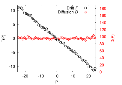
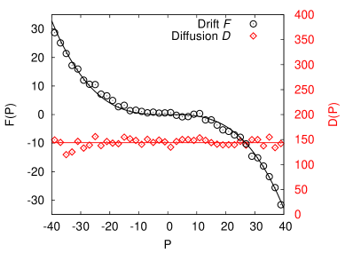
Figure 1: Drift and diffusion coefficients for the Langevin Equation describing $P$, inferred from simulations. Left: model (12) with $M=200$, $k=2500$, $2N=2000$, $\beta\simeq 1.0$; integration step $\delta t=10^{-3}$. Right: model (14) with $M=50$, $k=2500$, $2N=2000$, $\beta\simeq 0.45$; integration step $\delta t=4\cdot 10^{-4}$. Drifts are fitted with functions in the form (7), diffusivities with constant values.

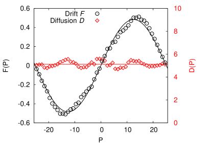
Figure 2: Drift and diffusion coefficients for the Langevin Equation describing $P$ in model (16), inferred from simulations. Left: $\beta=+0.11$; right: $\beta=-0.10$. In both cases $M=8$, $k=0.5$, $N=600$, $n=15$; integration step $\delta t=5\cdot 10^{-2}$. As in Fig. 1, drifts are fitted with functions in the form (7), diffusivities with constant values.

The results of our extrapolation procedure are shown in Figs. 1, 2. In all the considered cases, $D(P)$ is quite constant with respect to the momentum, therefore equation (7) applies; indeed, $F(P)$ seems to match quite well our phenomenological prediction.
Of course there is a pragmatic way to decide of the goodness of the above approach: compare the results from the LE and those obtained with the exact results of the deterministic system. In Fig. 3 we superimpose velocity autocorrelation functions and stationary p.d.f. obtained by stochastic simulations of the Langevin Equations to their deterministic analogues. The similarity between the two cases is quite evident.

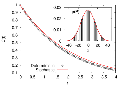
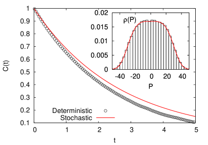
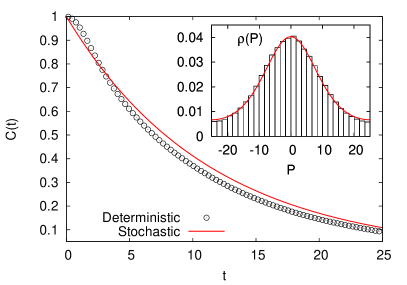
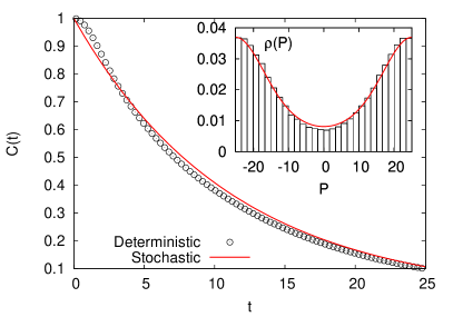
Figure 3: Autocorrelation functions for the velocity $\dot{Q}$ of the intruder in the same cases of Figs. 1, 2. Top-left: model (12); top-right: model (14); bottom-left: model (16) with $\beta>0$; bottom-right: model (16) with $\beta<0$. Black circles represent the outcomes of molecular dynamics simulations, solid red lines are computed by simulating Langevin Equations with the previously inferred coefficients. Insets: momentum p.d.f. from the same deterministic (histograms) and stochastic (solid red lines) simulations.

3.1 Some caveats

The hypothesis of a delta-correlated noise term in Eq. (17) is quite natural (in addition it is based on an old tradition); on the other hand one can wonder about the possibility of a non white noise: for instance, $\eta$ may be replaced by a stochastic process $s$ with a non zero correlation time $\tau$, described by

$${ds\over dt}=-{1\over\tau}s+c\eta\,.$$

At first, one can say that the agreement between the statistical features obtained with the Langevin equation and the numerical simulation is an indirect check of the validity of the assumption on the white noise. For a direct check one can compute the correlation function of the variable

$$Z(t)={dP(t)\over dt}-F(P(t))\,,$$ (19)

where $F(P)$ is determined by our fitting procedure and $P(t)$ is obtained by the numerical simulation.
In Fig. 6 (see Appendix) we show the correlation $C(t)=\langle Z(t)Z(0)\rangle$ in a particular case: since the dynamics is deterministic, $C(t)$ must be non zero for small $t$; on the other hand $C(t)\simeq 0$ for $t>t_{*}$ where $t_{*}$ is $O(\Delta t_{*})$, being $\Delta t_{*}$ the minimum value used in the fitting procedure to determine $F(P)$ and $D(P)$.
Beyond the numerical details, let us note that if a colored noise is present one can always describe the system with a Langevin equation with white noises including additional variables [36]. In other words the (possible) presence of colored noises is nothing but one of the difficulties whose relevance had been clearly stressed by Onsager and Machlup [34].

Let us also stress that a clear separation of the autocorrelation time-scales of our elected degree of freedom with respect to those of the other ones is not sufficient to apply blindly the above procedure. This can be related again to the caveat by Onsager and Machlup about the possible non Markovian character of the variable used to describe the slow motion [34].

As far as we know there are no protocols which allow for a sure decision, a priori, about the Markovian character of the dynamics; sometimes, however, some mathematical results can suggest that our guess is wrong. Let us consider the following system:

$$H=1-\cos(P/\sqrt{M})+\sum_{i=\pm 1,...,\pm N}[1-\cos(p_{i}/\sqrt{m})]+k\sum_{i=-N}^{N+1}[1-\cos(q_{i}-q_{i-1})],\quad\quad q_{-N-1}\equiv q_{N+1}\equiv 0,$$ (20)

where $P,q_{0}$ are momentum and position of the intruder. Note that this definition violates the mass additivity discussed in the paragraph before Eq. (14). In numerical simulations, for a given choice of parameters (see Fig. 4), we have observed that the ratio between the typical time of the intruder and that of the fast variable is $O(10)$, so one may hope that $P$ is described by a $1D$ Markov model. We have used the protocol discussed in Section III to build a Langevin equation for this model. The results can be appreciated in Fig. 4: we see that both the p.d.f. of $P$ and its autocorrelation in the reconstructed model are different from those of the real dynamics. In particular the autocorrelation is in clear disagreement. Such a negative conclusion could have been expected from the simple observation of the autocorrelation of $P$ in the real dynamics: there is a range of times $t$ where $C(t)<0$, a fact which is forbidden in $1D$ at equilibrium [5]. From the feature of numerically computed $C(t)$ and a rigorous mathematical result one has a sure indication that $P$ cannot be described by a $1D$ Markovian model. It is quite natural to guess that there exists a proper set of variables described by a Markovian rule, but unfortunately there is not a procedure to select such a set.

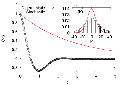
Figure 4: Results for the Hamiltonian in Eq. (20) for $M=200$, $k=2500$ $2N=2000$ and $\beta=1.04$ and the reconstructed Langevin equation. We show the autocorrelations of $\dot{Q}$ in the main graph, and its probability distributions in the inset.

4 Concluding remarks

In the present paper we introduced a practical procedure to build a Langevin equation for slow variables from a long time series, applying it to the data from simulations of Hamiltonian systems. Let us note that the use of such a protocol is not restricted to data from numerical simulations and can be exploited also with experimental results.
In addition we show that systems with negative temperatures does not exhibit any pathology: the dynamics of slow variables is described by a Langevin equation whose parameters can be computed with a well defined protocol. Such an effective equation is able to describe in a proper way the statistical features of the slow variables, including their dynamics.

As a final remark, we briefly comment about the very general problem of building models from data [37, 38, 39, 40]. Such an issue has attracted an increasing interest in the recent years, in particular in the context of the so-called Big Data paradigm and in the use of machine learning. Surely the simplest (and well posed) problem is that of building a model knowing the proper variables and the functional shape of the evolution equation, see for instance [38]. The task is more difficult when one knows the proper variables while the shape of the model is unknown [39]. The most ambitious problem is that of building a model using just data, without any a priori assumption about the structure of the equations and the relevant variables. An approach inspired to Takens has been used to write down evolution equations in ecological systems [40]; however such a procedure only works in low-dimensional systems [41]. The building of a LE, discussed here, is part of these challenges to extract models from data: a pragmatic attempt based on physical intuition and numerical treatment.

Appendix A Details on the numerical protocol

In this Appendix we discuss the numerical method we employ to infer drift and diffusion coefficients for the Langevin Equations of the heavy particle’s momentum. The idea is to perform molecular dynamics simulations of the Hamiltonian systems discussed in Section 3, in order to compute the limits (18) from averages on long time series of data.
All simulations are prepared in equilibrium initial conditions. This is particularly relevant for the harmonic chain case, since this Hamiltonian system is integrable and by no chance it can reach the proper equilibrium p.d.f. starting from out-of-equilibrium conditions; in this case one has to properly distribute the total energy among the normal modes of the chain.
Let $I=(-\tilde{P},\tilde{P})$ be a typical range for the momentum of the heavy particle, $P(t)$, and let us divide it into $n$ intervals $I_{1},I_{2},...,I_{n}$ of equal lengths. During the simulation, our algorithm periodically checks for what $j$ (if any) the relation $P(t)\in I_{j}$ holds; then it stores the values of $P(t+\Delta t)-P(t)$ for several $\Delta t$. In order to avoid correlations, the delay between two measures has been chosen to be at least $2\tau$, where $\tau$ is the velocity autocorrelation time of the intruder. At the end of the process, conditional averages on the r.h.s. of Eqs. (18) are computed as functions of both $j$ and $\Delta t$, and the limit $\Delta t\to 0$ can be inferred.
Let us note that the mathematical limit $\Delta t\to 0$ in the definitions of drift and diffusion coefficients must be interpreted in a proper physical way. It is quite simple to show that the description of a deterministic system in terms of a Langevin equation cannot be completely accurate at any time scale, but only at times larger than a certain characteristic threshold.
This can be easily understood noting that in a deterministic system, for any normalized correlation function,

$$C_{D}(t)=1-{t^{2}\over\tau_{D}^{2}}+O(t^{3})\,;$$

on the contrary, for a system whose evolution is ruled by a LE one has

$$C_{L}(t)=1-{t\over\tau_{c}}+O(t^{2})\,.$$

From the comparison of the two correlation functions it follows that the Markovian approximation can be valid only for

$$t>t_{*}=O\Bigl{(}{\tau_{D}^{2}\over\tau_{c}}\Bigr{)}\,.$$

As an example we can mention the case of an intruder in the harmonic chain seen in section 3, for which some exact results can be used [6]: here $\tau_{D}=\sqrt{M/k}$ and $\tau_{c}=M/\sqrt{4km}$, so that the previous approximation only applies for $t>2\sqrt{m/k}$.
Of course in general it is not simple to find a priori $t_{*}$ and therefore determine the minimum acceptable value of $\Delta t$. In our numerical computations of the drift we adopt a rather pragmatic approach: for a given $P$ we use different $\Delta t$ and then extrapolate the result using values of $\Delta t$ which are not too small. Fig. 5 shows a typical situation: fortunately one has an easy natural way to perform the extrapolation, i.e. using a polynomial function to fit the data and considering its value for $\Delta t=0$. In our analysis we employ linear fits for the drift and parabolic ones for the diffusion.

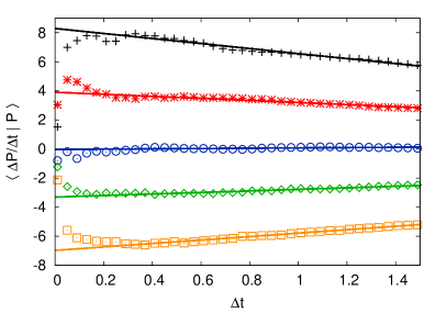
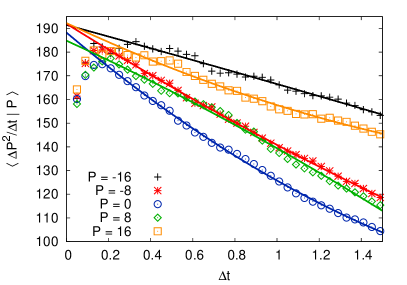
Figure 5: Extrapolating limits (18) for some values of $P$ (in the same conditions of Fig. 1). Drift (left) and diffusion (right) coefficients are inferred by considering linear and parabolic fits, respectively. The considered data interval for each fit is, in this case, $\Delta t\in[0.25,1.5]$.

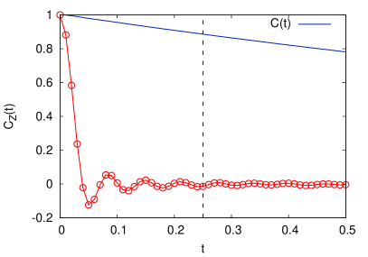
Figure 6: Autocorrelation of the $Z(t)$ function defined by Eq. (19) for model (12) (red circles), in the same conditions of Fig. 5. Velocity correlation function $C(t)$ (blue solid line) is shown for comparison; the minimum time interval that has been used in extrapolating the limits (18) is, in this case, $\Delta t_{*}=0.25$ (dashed vertical line).

With the aim of verifying that the noise is fairly approximated by a delta-correlated process, we compute the autocorrelation of the quantity $Z(t)$ defined in (19), whose plot is shown in Fig. 6. We see that indeed the “noise” $Z(t)$ loses memory in a time clearly smaller than $\Delta t_{*}$, the minimum value of $\Delta t$ we consider for the extrapolations (see dashed line), and certainly much smaller than the correlation time of the slow variable $P$.

To check the goodness of our extrapolation method one could, of course, compare the results to the analytical predictions valid for $M/m\rightarrow\infty$ in the thermodynamical limit. In this case, anyway, the resulting deviation of the measured values from the theoretical ones would be affected not only by the actual errors in the extrapolation procedure, but also by the fact that considering $P(t)$ as a stochastic process is by itself an approximation. At least in the case of the harmonic chain, however, we can do better than this: since the conditional p.d.f of $P$ is known, there is an easy way to compute the Langevin parameters from data without performing the limit $\Delta t\rightarrow 0$, and we can compare these values to the results of the previous method in order to estimate the precision of the extrapolation.

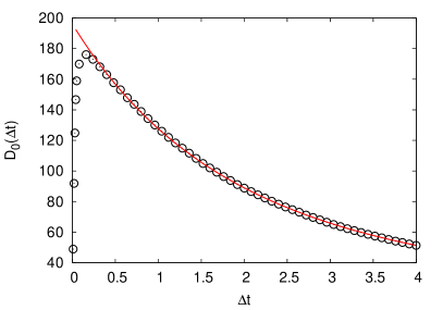
Figure 7: Evolution of $D_{0}(\Delta t)$ with the time interval. The red line is the result of a fit with the functional form (23).

To this end, let us note that since the conditional p.d.f. of $P$ is given by [12]:

$$f(P(t+\Delta t)|P(t))=\frac{1}{\sqrt{2\pi k_{B}TM(1-C(\Delta t)^{2})}}\exp\left\{-\frac{[P(t+\Delta t)-P(t)C(\Delta t)]^{2}}{2k_{B}TM(1-C(\Delta t)^{2})}\right\}\,,$$ (21)

we can explicitly compute the averages in Eq. (18), assuming that the Markovian limit holds and that the autocorrelation function actually verifies $C(\Delta t)=\exp(-\Delta t/\tau)$ for some $\tau$. For the diffusion term we get

$${1\over\Delta t}\langle\Delta P(\Delta t)^{2}|P(t)=P\rangle=D_{0}(\Delta t)+D_{1}(\Delta t)P^{2}\,$$ (22)

where

$$D_{0}(\Delta t)=\frac{k_{B}TM}{\Delta t}\left(1-e^{-2\Delta t/\tau}\right)\,,\quad\quad D_{1}(\Delta t)=\frac{\left(1-e^{-\Delta t/\tau}\right)^{2}}{\Delta t}P^{2}\,.$$ (23)

We can fit our data with the previous formula: in particular, from the fit of $D_{0}(\Delta t)$ (Fig. 7), we infer both $T$ and $\tau$ and calculate the corresponding values of drift and diffusion for Brownian motion [5],

$$F(P)=-P/\tau\,,\quad\quad D(P)=2Mk_{B}T/\tau\,.$$

The resulting values and the previously extrapolated coefficients differ by less than 3%, which is a quite satisfactory precision for our qualitative analysis.

Bibliography

Bibliography

- [1] van Kampen N G 2007 Stochastic Processes in Physics and Chemistry (Elsevier)
- [2] Livi R and Politi P 2017 Nonequilibrium Statistical Physics: A Modern Perspective (Cambridge University Press)
- [3] Langevin P 1908 C. R. Acad. Sci. (Paris) 146 530
- [4] Lemons D S 1997 Am. J. Phys. 65 1079
- [5] Gardiner C W 2009 Stochastic Methods (Springer Berlin)
- [6] Zwanzig R 2001 Nonequilibrium Statistical Mechanics (Oxford University Press)
- [7] Castiglione P, Falcioni M, Lesne A and Vulpiani A 2008 Chaos and coarse graining in statistical mechanics (Cambridge University Press)
- [8] Von Smoluchowski M 1906 Annalen der physik 326 756–780
- [9] Cecconi F, Cencini M and Vulpiani A 2007 J. Stat. Mech. 2007 P12001
- [10] van Kampen N 1961 Canad. J. Phys. 39 551
- [11] Sarracino A, Villamaina D, Costantini G and Puglisi A 2010 J. Stat. Mech. 2010 P04013
- [12] Rubin R J 1960 Journal of Mathematical Physics 1 309
- [13] Turner R 1960 Physica 26 269 – 273
- [14] Zwanzig R 1973 Journal of Statistical Physics 9 215–220
- [15] Seifert U 2012 Rep. Progr. Phys. 75 126001
- [16] Krüger M and Maes C 2017 J. Phys.: Condens. Matter 29 064004
- [17] Basu U, Maes C and Netočný K 2015 Phys. Rev. Lett. 114 250601
- [18] Cerino L, Puglisi A and Vulpiani A 2015 J. Stat. Mech. 2015 P12002
- [19] Puglisi A, Sarracino A and Vulpiani A 2017 Phys. Rep. 709-710 1
- [20] Baldovin M, Puglisi A, Sarracino A and Vulpiani A 2017 J. Stat. Mech. 2017 113202
- [21] Braun S, Ronzheimer J P, Schreiber M, Hodgman S S, Rom T, Bloch I and Schneider U 2013 Science 339 52–5
- [22] Kleinhans D, Friedrich R, Nawroth A and Peinke J 2005 Phys. Lett. A 346 42
- [23] Friedrich R, Peinke J, Sahimi M and Tabar M 2011 Phys. Rep. 506 87
- [24] Ragwitz M and Kantz H 2001 Phys. Rev. Lett. 87 254501
- [25] E W, Engquist B, Li X, Ren W and Vanden-Eijnden E 2007 Commun. Comput. Phys. 2 367
- [26] Givon D, Kupferman R and Stuart A 2004 Nonlinearity 17 R55
- [27] Kifer Y 2004 Some recent advances in averaging Modern Dynamical Systems and Applications ed Brin M, Hasselblatt B and Pesin Y (Cambridge: Cambridge University Press) p 385
- [28] MacKay R S 2010 Langevin equation for slow degrees of freedom of hamiltonian systems Nonlinear dynamics and chaos: advances and perspectives ed Thiel M, Kurths J, Romano M C and ad A Moura G K (Springer) p 89
- [29] Friedrich R, Renner C, Siefert M and Peinke J 2002 Phys. Rev. Lett. 89 149401
- [30] Takeno S and Hori J 1962 Progress of Theoretical Physics Supplement 23 177–184
- [31] Mazur P and Braun E 1964 Physica 30 1973–1988
- [32] Ford G W, Kac M and Mazur P 1965 Journal of Mathematical Physics 6 504–515
- [33] Iubini S, Franzosi R, Livi R, Oppo G L and Politi A 2013 New J. Phys. 15 023032
- [34] Onsager L and Machlup S 1953 Phys. Rev. 91 1505
- [35] Ma S K 1985 Statistical Mechanics (World Scientific Publishing)
- [36] Villamaina D, Baldassarri A, Puglisi A and Vulpiani A 2009 Journal of Statistical Mechanics: Theory and Experiment 2009 P07024
- [37] Chibbaro S, Rondoni L and Vulpiani A 2014 Reductionism, Emergence and Levels of Reality (Springer-Verlag)
- [38] Pikovsky A 2017 arXiv:1711.06453
- [39] Pathak J, Lu Z, Hunt B, Girvan M and Ott E 2017 arXiv:1710.07313
- [40] Ye H, Beamish R, Glaser S, Grant S, Hsieh C, Richards L, Schnute J and Sugihara G 2015 Proceedings of the National Academy of Sciences 112 E1569
- [41] Cecconi F, Cencini M, Falcioni M and Vulpiani A 2012 American Journal of Physics 80 1001