QUALITATIVE ANALYSIS OF

DIFFERENTIAL EQUATIONS

Alexander Panfilov

Chapter 1 Preliminaries

1.1 Basic algebra

1.1.1 Algebraic expressions

Algebraic expressions are formed from numbers, letters and arithmetic operations. The letters may represent unknown variables, which should be found from solutions of equations, or parameters (unknown numbers) on which the solutions depend.

Below, we review examples several basic operations which help us to work with algebraic express of ions.

One of the most basic algebraic operations is opening of parentheses, or simplification of expressions. For that we use the following rule:

$$(a+b)*(c+d)=ac+ad+bc+bd$$

note, that here $ac$ means $a*c$, etc., as in algebra the multiplication is often omitted.

Example (open parenthesis): $(4x+2a)(2-3x)=8x-12x^{2}+4a-6ax$

Sometimes we use parentheses to factor expressions:

Example (factor expression): $9x^{3}+3x^{2}-6a^{4}x^{2}=x^{2}(9x+3-6a^{4})=3x^{2}(3x+1-2a^{4})$

In many cases we also need to work with fractions:

Example (the same denominator): ${a^{2}-ca\over 3}={a^{2}\over 3}-{ca\over 3}$

Example (different denominators): ${a^{2}\over b}+{b\over a}={a^{2}\over b}{a\over a}+{b\over a}{b\over b}={a^{2}*a\over ab}+{b*b\over ab}={a^{3}+b^{2}\over ab}$

Example (fractions simplifications): ${a^{2}-ca\over 3a}={a-c\over 3}$

To divide a fraction ${a\over b}$ by another fraction ${c\over d}$ we just need to multiply it by its inverse ${d\over c}$: ${a\over b}:{c\over d}={a\over b}*{d\over c}={ad\over bc}$,

Example (division): ${4\over 7}:{2a\over 5}={4\over 7}{5\over 2a}={20\over 14a}={10\over 7a}$

Also note that: ${x+y\over z+d}\mathbf{\neq}{x\over z}+{y\over d}$

1.1.2 Limits

We call $A$ a limit of the function $f(x)$ when $x$ approaches $a$, if the value of $f(x)$ get closer and closer to $A$ when $x$ takes values closer and closer to $a$. We write it formally as:

$$\mathop{\lim}\limits_{x\to a}f(x)=A$$ (1.1)

In many cases, finding the limit is trivial: we just need to substitute the value of $x=a$ into our function:

$${\lim_{x\rightarrow a}}f(x)=f(a)$$ (1.2)

Example: $\mathop{\lim}\limits_{x\to 2}\quad x^{3}=2^{3}=8$

Functions which have such property are called continuous and most of the functions used in biology are continuous. However, there are several important exception.

The first case, which will be the most important for us, is finding of limit of the function when $x\rightarrow\infty$. Finding such limits is important as it gives an asymptotic behaviour of our system when the size of a population becomes very large. Unfortunately, there is no such number ’$\infty$’ which we can substitute into our function to find a limit using formula (1.2). For functions without parameters, we can guess the limit by substituting large values to (1.2), e.g. $x=10000,20000,etc$, but what to do for functions with parameters?

Let us discuss this problem for a special class of functions, which are the most relevant to our course, the so called rational functions $f(x)={p(x)\over g(x)}$, where $p(x)$ and $g(x)$ are polynomials. In that case we can always find the limit using the following property of the power function:

$${\lim_{x\rightarrow\infty}}{C\over x^{\alpha}}=0$$ (1.3)

where $C$ is an arbitrary constant and $\alpha>0$.

To prove it note that if $x$ approaches $\infty$ (becomes larger and larger), the power function $x^{\alpha}$ with $\alpha>0$ also becomes larger and larger and therefore ${C\over x^{\alpha}}$ will be closer and closer to zero, thus in accordance with the definition $\mathop{\lim}\limits_{x\to\infty}{C\over x^{\alpha}}=0$

To find the limit using this rule we need to do the following: (1) find the highest power of $x$ in our expression ${p(x)\over g(x)}$, (2) divide each term in our function by $x$ in that power, and (3) find the limit of each term using property (1.3). Let us consider three typical examples:

Example (find the limit): $\mathop{\lim}\limits_{N\to\infty}{aN^{2}-3N\over 3-2N^{2}}$.

The highest power is $N^{2}$, division gives: ${{aN^{2}\over N^{2}}-3{N\over N^{2}}\over{3\over N^{2}}-{2N^{2}\over N^{2}}}={{a}-{3\over N}\over{3\over N^{2}}-{2}}$. The limits of the individual terms are: ${{a}-0\over 0-2}=-{a\over 2}$

Example (find the limit): $\mathop{\lim}\limits_{P\to\infty}{aP-3bP^{3}\over cP-dP^{2}}$, $a,b,c,d\neq 0$.

Similar steps give us: ${aP-3bP^{3}\over cP-dP^{2}}={{aP\over P^{3}}-{3bP^{3}\over P^{3}}\over{cP\over P^{3}}-{dP^{2}\over P^{3}}}={{a\over P^{2}}-{3b}\over{c\over P^{2}}-{d\over P}}={0-{3b}\over 0-0}={-{3b}\over 0}$. This expression does not have sense as we cannot divide by zero and we do not have a finite limit for this function.

Example (find the limit): $\mathop{\lim}\limits_{x\to\infty}{ax^{3}-bx^{2}+c\over ax^{4}-b}$,         $a,b,c\neq 0$ .

${ax^{3}-bx^{2}+c\over ax^{4}-b}={{ax^{3}\over x^{4}}-{bx^{2}\over x^{4}}+{c\over x^{4}}\over{ax^{4}\over x^{4}}-{b\over x^{4}}}={{a\over x}-{b\over x^{2}}+{c\over x^{4}}\over{a}-{b\over x^{4}}}={0-0+0\over{a}-0}={0\over a}=0$.

Another non-trivial situation occurs when the denominator of our function $f(x)={p(x)\over g(x)}$ becomes zero for some value of $x$, for example $f(x)={2\over x-3}$ for $x=3$. In this case the formula (1.2) for limit cannot be used and other more careful analysis is necessary. If using of calculator we substitute some numbers into our function around point $3$ we will find the following: if $x$ becomes closer and closer to $3$ from the left, e.g. $x=3.1;3.05;3.01,3.005;etc$ the function value becomes larger and larger, while if $x$ becomes closer and closer to $3$ from the right, e.g. $x=2.9;2.95;2.99,2.995;etc$ the function value is negative and its absolute value also becomes larger and larger. We can formally write it as $\mathop{\lim}\limits_{x\to 3^{+}}{2\over x-3}=+\infty$, while $\mathop{\lim}\limits_{x\to 3^{-}}{2\over x-3}=-\infty$. However, in a strict sense, as there is no real number for which $f(x)$ approaches for $x$ close to $3$ (from either side) thus the limit here does not exist.

We will use limits for drawing our functions and will see that limits at infinity give us horizontal asymptotes of our graphs, while blow up of functions for some $x$ (as in the last example) give us vertical asymptotes.

1.1.3 Equations

An equation is a mathematical relationship involving unknown variables. These unknowns are usually expressed by letters ’x’, ’y’, however in biology we use many other letters (e.g. ’N’, ’P’. ’T’, ’V’, etc.), which maybe somewhat related to the name of the species they describe. Solving equations means finding unknown(s) such that after substitution in the equation the left and right hand sides will be equal to each other. For example: equation $2x-16=-10$ has a solution $x=3$, as $2*3-16=6-16=-10$.

The usual way to solve equations which have unknown variables in the first power only (linear equations), is to isolate the unknowns:

$$x=[known\;numbers]$$

We can achieve that by using the following rules of equation algebra: (1) we can multiply, or divide both sides of the equation by the same number, and (2) we can move numbers/expressions from one to the other side of the equation, by changing their sign. The proof of these rules is trivial. Indeed if two expressions are the same $X=Y$, then if we multiply (or divide) both of them by the same number $a$, they still will be the same $aX=aY$. Similarly if $X=Y+a$, we can add $-a$ to the both sides of the equation, which will not change the equality, but we get: $X-a=Y+a-a$, or $X-a=Y$. Thus we see, that we were able to move $a$ from the right hand side to the left hand side of our equation, but it changed its sign as a result.

Example(solve equation): $4-2x=2-4x$.

Solution:$-2x+4x=2-4\quad 2x=-2\quad x=-1$

For a quadratic equation $ax^{2}+bx+c=0$ we use the ’abc’ formula, which gives us the solutions as $x_{1,2}={-b\pm\sqrt{b^{2}-4ac}\over 2a}$.

Example (solve equation): $x+1={4\over 1+x}$.

Solution: $(1+x)(x+1)=4\quad 1+x+x^{2}+x=4;\quad x^{2}+2x+1-4=0;\quad x^{2}+2x-3=0$ from the ’abc’ formula $x_{1,2}={-2\pm\sqrt{4-4*1*(-3)}\over 2}={-2\pm\sqrt{16}\over 2}={-2\pm 4\over 2}\quad x_{1}=1;x_{2}=-3$.

Equation may also contain parameters. A parameter is an unknown number (constant) that may have any value. It is different from the unknown variable, as the parameter is just a constant on which our solution depends.

Example (solve equation): $a{k\over P^{2}}-dP=0$, where $P$ in unknown variable and $a,k,d>0$ are parameters.

Solution: By multiplying both sides by $P^{2}$ we get $ak-dP*P^{2}=0$, or $ak=dP*P^{3}$, or $P^{3}={ak\over d}$, thus $P=\sqrt[3]{{ak\over d}}$. We see that the solution depends on 3 parameters and if someone provides us with their values we will be able to find the solution by substituting the parameter values into the final formula.

1.1.4 Systems of equations

To solve a system of two linear equations we express one variable via the other and substitute it into the other equation.

Example (solve the system of equations): $\left\{\begin{array}[]{l}2x+y=5\\ x+y=3\end{array}\right.$

Solution: From the second equation we find $x=3-y$, so we substitute $x$ into the first equation: $2(3-y)+y=5;\quad 6-2y+y=5;\quad-y=-1;\quad y=1$, now substitute this value to $x=3-y$ and find $x=3-1-2$, thus the solution is $x=2,y=1$.

Unfortunately, there are no general rules to solve a system of nonlinear equations. The usual practical way is to start with a more simple equation, try to obtain from it as much information as possible and then substitute it to the other equation. It is also very helpful to factor expressions in order to simplify them.

Example (solve the system of equations): $\left\{\begin{array}[]{l}2n-2n^{2}-2np=0\\ np-2p=0\end{array}\right.$

Solution: From the second equation by factoring we find $np-2p=p(n-2)=0$. The product is zero only if one of the multipliers is zero, thus we have two possibilities $p=0$ or $n=2$. If we substitute $p=0$ into the first equation we find $2n-2n^{2}-0=0$, or $2n(1-n)=0$, thus for $p=0$ we have two solutions $n=0$, or $n=1$; now substitute $n=2$ into the first equation: $2*2-2*4-2*2*p=0$, $4-8-4p=0$, $-4p=4$, thus for $n=2$ we found $p=-1$. Overall, we found the following three solutions of the given system $(n=0,p=0),(n=1,p=0),(n=2,p=-1)$.

Systems may also contain parameters.

Example (solve the system): $\left\{\begin{array}[]{l}an-an^{2}-bnp=0\\ np-kp=0\end{array}\right.$, where $n,p$ are variables and $a,b,k>0$, are the parameters.

Solution: We proceed similarly as in the previous case. From the second equation: $np-kp=p(n-k)=0$, thus we have two cases $p=0$ or $n=k$. After substituting $p=0$ into the first equation we get: $an-an^{2}-0=0$, $an(1-n)-0$, thus $n=0$, or $n=1$; after substituting $n=k$ into the first equation we get: $ak-ak^{2}-bkp=0$, $ak(1-k)=bkp$, $a(1-k)=bp$, thus $p={a(1-k)\over b}$. Therefore, we found three solutions: $(n=0,p=0),(n=1,p=0),(n=k,p={a(1-k)\over b})$. It is easy to see that if we substitute the parameter values $a=2,b=2,k=2$ to these formulas we obtain the solution of the previous problem. Note also, that for systems with parameters we need to be careful as not all operations are allowed for arbitrary parameter values. In our example in order to obtain the solution we had to make several divisions by parameters $a,b$, and $k$. However we can always do that as the parameters are positive numbers ($a,b,k>0$) and thus they cannot be equal to zero.

Finally note, that we can solve systems of three and more equations similarly, by subsequent substitutions from one equation to another, etc..

1.2 Functions of one variable

In science the relationships between quantities are normally expressed using functions. The simplest type of functions are functions of one variable. The function of one variable $f$ is a rule that allows us to find the value of a variable (number) $f$ from a single variable (number) $x$. We denote it as $f(x)$. Below are examples of the most important functions:

1. power functions $x^{a}$, for example

   $$f(x)=x^{1\over 2}=\sqrt{x};\;\;\;f(x)=x^{-2}={1\over x^{2}}.$$ (1.4)

2. polynomials, $ax^{3}+..+cx+d$, for example:

   $$f(x)=3x^{3}-2x^{2}+1$$ (1.5)

3. rational functions $f(x)={p(x)\over g(x)}$:

   $$f(x)={2-x\over x^{2}+1}$$ (1.6)

4. trigonometric functions $sin$, $cos$, $tan$:

   $$f(x)=2*sin(x);\;\;f(x)=cos(2x-1);\;\;f(x)=tan({x\over 2})$$ (1.7)

5. exponential $a^{x}$ and logarithmic function ${}^{a}log(x)$

   $$f(x)=e^{x+1};\;\;f(x)=^{10}log(2x);\;\;f(x)=2^{2x}\;\;$$ (1.8)

6. etc.

The derivative of a function $f(x)$ at point $x^{*}$ is given by the following limit:

$$f^{\prime}(x^{*})={df\over dx}=\mathop{\lim}\limits_{x\to x^{*}}{f(x)-f(x^{*})\over x-x^{*}}$$ (1.9)

The derivative $f^{{}^{\prime}}(x^{*})$ shows the rate of change of a function $f(x)$ at a point $x^{*}$ and has many important applications:

• If x(t) is the distance traveled by a car as a function of time $t$, then $dx/dt$ gives the velocity of the car.

• If $n(t)$ is the size of a population as the function of time, then $dn/dt$ gives the rate of growth of the population.

Geometrically, the derivative $f^{{}^{\prime}}(x^{*})$ gives the slope of the tangent line to the graph of the function at the point $x^{*}$ (fig.1.1).

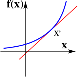
Figure 1.1:

A graph of a line tangent to the function $f(x)$ at point $x^{*}$ (fig.1.1) is given by the following equation:

$$y=f(x^{*})+f^{\prime}(x^{*})*(x-x^{*})$$ (1.10)

Equation (1.10) is also known as a linear approximation of function $f(x)$ at point $x^{*}$:

Let us check formula (1.10) by approximating the function $y=2x^{2}+1$ at $x^{*}=1$. We find: $f(x^{*})=2*1^{2}+1=3,\;f^{\prime}=4x,\;f^{\prime}(1)=4$, hence $f(x)\approx 3+4*(x-1)$. At $x=1.1$ this approximate formula gives $f(1.1)\approx 3+4*(1.1-1)=3.4$. The exact value is $f(1.1)=2*1.1^{2}+1=3.42$. So the error is just 0.6%. However, if $x=0,\;f(0)\approx 3+4*(0-1)=-1$ while the exact value is $f(0)=1$. So we see, that the approximate formula works good if $x$ is close to $x^{*}$ only.

Functions with parameters. Functions may depend not only on variable(s) but also on parameters. We have already seen the following example of the function $f(x)$ that depends on three parameters $a,b,c$:

$$f(x)=ax^{2}+bx+c$$ (1.11)

Equation (1.11) describes a general quadratic polynomial. If we choose, for example $a=3,b=-2,c=1$ we will get the function given by equation (1.5). Studying functions with parameters allows us to obtain results for whole classes of functions. We will frequently use functions with parameters in our course. This is because biological models usually depend on many (up to hundreds) parameters and in many situations the exact values of these parameters are unknown. One of practical difficulties in working with parameters is that use of calculators is very limited, because calculators cannot do calculations with unknown quantities. The most valuable methods to study functions with parameters are direct algebraic computations and analysis of the obtained formulas. In this course we will widely use the graphical methods of representation of function. Let us start with review of the basic function graphs.

1.3 Graphs of functions of one variable

Example of graphs. We usually represent functions using graphs. To do that we plot the value of the variable $x$ along the $x$-axis and the value of the function $f(x)$ along the $y$-axis. Let us start first by listing typical graph shapes that are important in this course.

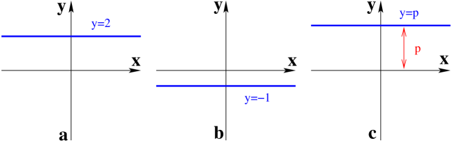
Figure 1.2:

Equation $y=p$ produces a horizontal line at the level $p$ (fig.1.2).

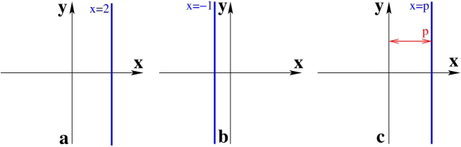
Figure 1.3:

Equation $x=p$ produces a vertical line shifted by $p$ from the $y$-axis (fig.1.3)

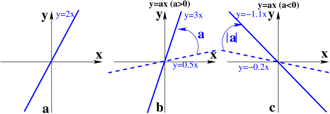
Figure 1.4:

Equation $y=ax+p$ (linear function) produces a straight line with the slope defined by the parameter $a$: the larger the absolute value of $a$, the steeper is the slope (fig.1.4).

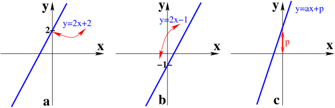
Figure 1.5:

The parameter $p$ in $y=ax+p$ accounts for the vertical shift of the graph fig.1.4.

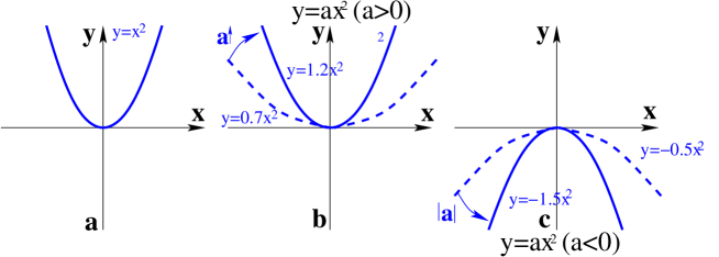
Figure 1.6:

Equation $y=ax^{2}$ produces a parabola, if $a>0$ the parabola is opened upward (fig.a,b), and if $a<0$ the parabola is opened downward (fig.c). The larger the absolute value of $a$ is, the steeper is the parabola.

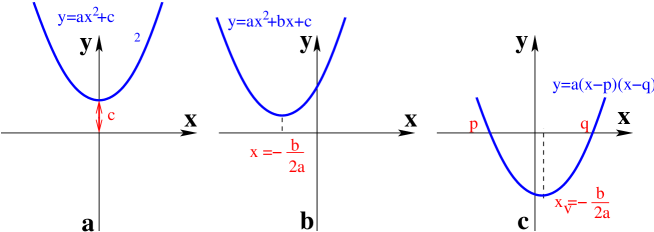
Figure 1.7:

Equation $y=ax^{2}+bx+c$ also produces a parabola. Parameter $c$ (fig.1.7a) accounts for the vertical shift of the graph. Parameter $b$ accounts for a horizontal shift of the parabola. It is possible to show that the horizontal shift of the parabola is given by $-{b\over 2a}$ (fig.1.7b). We can calculate this shift by determining the location of the vertex of the parabola which is a point of extremum (maximum or minimum) of the function. At this point the derivative of the function to zero $(ax^{2}+bx+c)^{\prime}=2ax+b=0$, Thus the $x$ coordinate of the vertex is given by $x_{v}=-{b\over 2a}$, or in other words the (vertex of) parabola is shifted by $x_{v}=-{b\over 2a}$ from its central location in (fig.1.7a. Note also, that a parabola may have up to two points of intersection of the graph with the $x$-axis (zeros of the function). They can be found from the ’abc’ formula for roots of the equation $ax^{2}+bx+c=0$, and if these roots ($p,q$) are known, the graph can easily be depicted using them (fig.1.7c). Note, that in this case the vertex of the parabola is always located at the middle between these two roots.

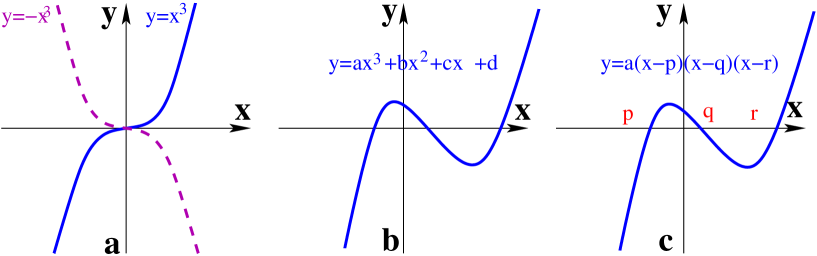
Figure 1.8:

For a general cubic function $y=ax^{3}+bx^{2}+cx+d$ we have much more possibilities and we will not discuss all of them here. The two basic forms are given by the functions $y=x^{3}$ and $y=-x^{3}$ depicted in Fig.1.8a. Important here is the asymptotic behavior of the function at $x\rightarrow\pm\infty$. For $y=x^{3}$ we see that $y$ goes to $+\infty$ when $x$ increases and to $-\infty$ when $x$ decreases; for $y=-x^{3}$ we have the opposite situation. A general graph of $y=ax^{3}+bx^{2}+cx+d$ may have up to three zeros that can be found from the solution of the equation $ax^{3}+bx^{2}+cx+d=0$, and up to two extrema (fig.1.8b). The extrema are points where the derivative of the function is zero, which in this case results in the following quadratic equation: $(ax^{3}+bx^{2}+cx+d)^{\prime}=3ax^{2}+2bx+c=0$. If the zeros of the function $(p,q,r)$ are known, the graph can easily be drawn as shown in Fig.1.8c.

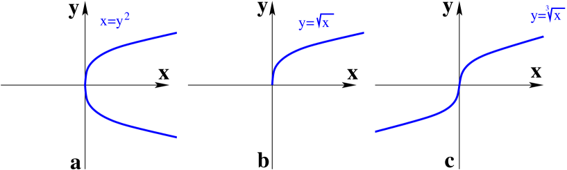
Figure 1.9:

Three examples of graphs of the power function $x^{a}$ involving fractional powers are shown in Fig.1.9. If $0<a<1$ than the graph growth is slower than the function $y=x$ and is concave downward (in the first quadrant). To draw graph $y=\sqrt{x}$ let us use the graph of parabola $y=x^{2}$ discussed in Fig.g1d5a. If in function $y=x^{2}$ we switch the $x$ and $y$ we will get $x=y^{2}$, which is equivalent to $y=\pm\sqrt{x}$. The graph $x=y^{2}$ can be found by switching the $x$ and the $y$-axis for the graph of the parabola $y=x^{2}$ in Fig.1.6a and we get a curve depicted in fig.1.9a in which the upper branch corresponds to $y=\sqrt{x}$ (fig.1.9b) and the lower branch corresponds to $y=-\sqrt{x}$. Similarly, the graph of the function $y=\sqrt[3]{x}$ (Fig.1.9c) can be found by a $90^{o}$ rotation of the graph of the function $y=x^{3}$ from Fig.1.8a.

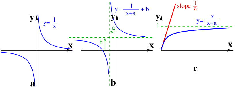
Figure 1.10:

Rational functions ${p(x)\over q(x)}$ are very important in theoretical biology. The graph of the function $y={1\over x}$ (Fig.1.10a) has the vertical asymptote ($x=0$) and the horizontal asymptote ($y=0$). The graph of function $y={1\over x+a}+b$ can be obtained by a shift of the graph $y={1\over x}$ by $b$ units in the $y$ (vertical) direction and by $-a$ units in the $x$ (horizontal) direction. In this case the vertical asymptote ( $x$ at which function goes to infinity) is $x=-a$, as at this point the denominator in ${1\over x+a}$ equals zero. The horizontal asymptote of this graph is $y=b$, given by $\mathop{\lim}\limits_{x\to\infty}{1\over x+a}+b=b$. Another rational function $y={x\over x+a}$ occurs in the classical Michaelis-Menten kinetics. Fig.1.10c shows the graph of this function. Because for biological applications $x$ and $a$ are always considered non-negative ($x\geq 0,a>0$), we show the graph in the first quadrant only. We see that independent of the value of the parameter $a$ the horizontal asymptote is always located at $y=1$, as $\mathop{\lim}\limits_{x\to\infty}{x\over x+a}=1$. The slope of this function at $x=0$ is given by the function derivative $f^{\prime}(x)=({x\over x+a})^{\prime}={a\over(x+a)^{2}}$ at $x=0$, which gives a slope of $f^{\prime}(0)={1\over a}$.

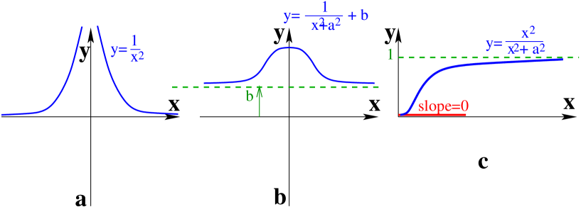
Figure 1.11:

Graphs of similar functions involving a second power: $y={1\over x^{2}}$ and $y={1\over x^{2}+a^{2}}$, are shown in Fig.1.11a,b. We see that function $y={1\over x^{2}}$ has a graph similar to that of $y={1\over x}$ but located in the first and second quadrants, rather than first and third. One more difference is that function $y={1\over x^{2}+a^{2}}$ does not have a vertical asymptote, and always reaches a maximum at $x=0$. Function $y={x^{2}\over x^{2}+a^{2}}$ is an example of famous for its ecological applications Hill function $y={x^{n}\over x^{n}+a^{n}}$ with $n=2$. Its graph (Fig.1.11c) has a horizontal asymptote at $y=1$ (similar to $y={x\over x+a}$), however, the rate of growth of $y={x^{2}\over x^{2}+a^{2}}$ for small $x$ is slower than for $y={x\over x+a}$: the slope of the tangent line at $x=0$ here is $0$, which can be found from the derivative of this function.

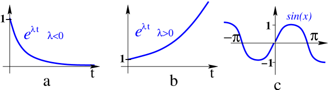
Figure 1.12:

Finally in fig.1.12 we show graphs of two other functions that are important in this course $e^{\lambda t}$ and $sin(x)$. Note that if $t$ grows the function $e^{\lambda t}$ approaches zero if $\lambda<0$ and diverges to infinity if $\lambda>0$. The function $sin(x)$ oscillates with a period of $2\pi$ between $-1$ and $+1$.

Tips on graphs

Let us list important rules that may help to plot graphs of function $y=f(x)$ with parameters.

$\bullet$ The graph of the function $y=f(x)+p$ can be obtained by a vertical shift by $p$ units of the graph of $y=f(x)$.

Example: In function ${N\over N+b}+c$, parameter $c$ just shifts the graph of ${N\over N+b}$ by $c$ units above.

$\bullet$ Important points of the graph are points at which the graph crosses the $y$-axis ($y$-intercept), given by $y=f(0)$, and points where the graph crosses the $x$-axis (zeros of the function), given by $f(x)=0$. Note, that some graphs do not cross the $x$ or the $y$ axis and thus do not have $y$-intercepts or zeros. For example graph of function $f(x)={1\over x}$ (Fig.1.10a) does not have finite zeros or $y$-intercepts.

Example: For function $f(N)={N\over N+b}+c,\;b,c>0$, the $y$-intercept is ${0\over 0+b}+c=c$. Zeros can be found from ${N\over N+b}+c=0$, which gives $N+c(N+b)=0$, or $N+cN+cb=0$, or $N(1+c)=-cb$, thus zero is given by the formula $N=-{cb\over 1+c}$, which is always valid as $c>0$.

$\bullet$ Another important graph feature are asymptotes. To find a horizontal asymptote we need to compute the $\mathop{\lim}\limits_{x\to\infty}f(x)$. For functions without parameters, you can try to compute this limit using calculator by filling in a large numbers 10000, 20000, etc and looking if the function approaches some constant value. For functions with parameter, you can try to fill in some ’reasonable’ parameter value and try to find similarly if the asymptote exists, however the best way here is to find the limit using our plan from section 1.1.2. A vertical asymptote is usually a point where a denominator of a fraction is zero. Not all graphs have asymptotes, for example graph of function $f(x)=x^{2}$ does not have any vertical or horizontal asymptotes. However, even if the asymptotes are absent it is still useful to understand behavior of the functions at large $x$ and show it in the graph.

Example: For function ${N\over N+b}+c$ we can find $\mathop{\lim}\limits_{N\to\infty}$ as ${N\over N+b}+c={{N\over N}\over{N\over N}+{b\over N}}+c={1\over 1+{b\over N}}+c={1\over 1+0}+c=1+c$, thus this graph has a horizontal asymptote $y=1+c$. The vertical asymptote here is at point where $N+b=0$, or line $N=-b$.

$\bullet$ Several features of the graph can be found from the derivative of the function: a function grows if its derivative $f^{\prime}(x)>0$, decreases if $f^{\prime}(x)<0$ and has a local extremum (maximum or minimum) if $f^{\prime}(x^{*})=0$. We do not necessarily need to compute these feature for each graph, but it may be helpful for some functions.

In many applications we will be interested in points of intersection of graphs of two functions $f(x)$ and $g(x)$. Because at the intersection point functions are equal to each other, such points can be found from the equation $f(x)=g(x)$.

The above mentioned tips are represented graphically in fig.1.13.

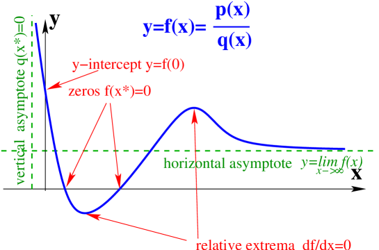
Figure 1.13:

Finally let us formulate the main rules for graphing functions with parameters.

Plan for graphing functions with parameters

1. Try to simplify the function and determine if it belongs to a known class of functions with graphs from (Fig.1.2-1.11).

2. Computer trail:

   1. Put parameters to ’reasonable’ values and plot the graph using a calculator.

   2. Collect qualitative information such as : number of zeros, existence of vertical and horizontal asymptotes.

   3. Vary parameter values to see how this changes the shape of the graph.

3. Algebraic approach (note, not all steps may be possible):

   1. Find $y$-intercept ($f(0)$), and zeros of the function ($f(x)=0$).

   2. Find horizontal asymptote from the limit $y=\mathop{\lim}\limits_{x\to\infty}f(x)$ and vertical asymptote(s) (for rational function ${p(x)\over q(x)}$ they are at the points where the denominator becomes zero ($q(x)=0$)) ( fig.1.13).

   3. Find other special points (e.g. maximum, minimum, etc), if they are important determinants of the graph shape.

   4. Draw the graph and indicate how the graph shape changes for different parameter values.

Example Plot the graph of the function $f(x)={ax\over x^{2}+c^{2}}\;\;x\geq 0\;\;\;\;a>0\;c>0$. Find how the graph depends on the parameters $a$ and $c$

Solution.

1. We do not need to simplify the function. The function equation has some similarities with graph classes listed above, but does not coincide exactly with any of them.

2. Let us put $a=c=1$ and plot the graph using calculator (fig.1.14a).

3. The graph (fig.1.14a) has the following characteristic features: the $y$-intercept here is $y=0$, we see one zero of the function $x=0$. If we fill in large values of $x$, we find that $f(1000)=0.00099$,$f(5000)=0.000199$ and $f(10000)=0.00009$, thus we expect to have a horizontal asymptote $y=0$, we do not see any vertical asymptotes and function has an extremum point (maximum). However, will these features persist for other parameter values? In order to answer that let us perform an algebraic study.

4. $y$-intercept is $f(0)={a*0\over 0^{2}+c^{2}}=0$. Zeros of the function are given by ${ax\over x^{2}+c^{2}}=0$, which has only one solution $x=0$, as $x^{2}+c^{2}\neq 0$ for all $x$.

5. The function does not have vertical asymptotes as the denominator cannot be zero ($x^{2}+c^{2}>0$ for all $x$ and $c>0$). To find the horizontal asymptote let us compute $y=\mathop{\lim}\limits_{x\to\infty}{ax\over x^{2}+c^{2}}=\mathop{\lim}\limits_{x\to\infty}{{a\over x^{2}}\over{x^{2}\over x^{2}}+{c^{2}\over x^{2}}}={0\over 1+0}=0$, thus the horizontal asymptote is the $x$-axis.

6. Important point here is the location of the maximum of the function. Let us find it. For that let us find the points where the derivative of the function is zero. The derivative of the function is $f^{\prime}(x)={a*(x^{2}+c^{2})-2x*ax\over(x^{2}+c^{2})^{2}}={ac^{2}-ax^{2}\over(x^{2}+c^{2})^{2}}=0$, thus the expression is zero if $ac^{2}-ax^{2}=0$, or $x=\pm c$. For $x\geq 0,c>0$ we have just one solution $x=c$. The value of the function at this extreme point is $f(c)={ac\over c^{2}+c^{2}}={a\over 2c}$, thus the maximum is at $(c,{a\over 2c})$.

7. Let us draw the graph now. Because $f(0)=0$ the graph always goes through the origin. Then the graph will reach the maximum at $(c,{a\over 2c})$ (Fig.1.14a, symbol ’1’) and then approaches the $x$ axis. If we put all this information together we obtain a qualitative graph shown in fig.1.14b. We see that it qualitatively coincides with the calculator sketch. Now let us find how the graph shape depends on the parameter values. We see that the graph has a bell-shape, with a single maximum at $(c,{a\over 2c})$. The $x$ location of this maximum depends on the parameter $c$ only, but the maximal value of the function increases if $a$ increases. The solid and the dashed line in Fig.1.14c illustrate how the graph shape changes if $a$ increases while we keep $c$ constant. Alternatively, if we keep the $a$ value constant but increase the value of the parameter $c$ (the solid and the dot-dashed line in fig.1.14c), the $x$ location of the maximum shifts to the right, and the maximal value of the function ${a\over 2c}$ decreases.

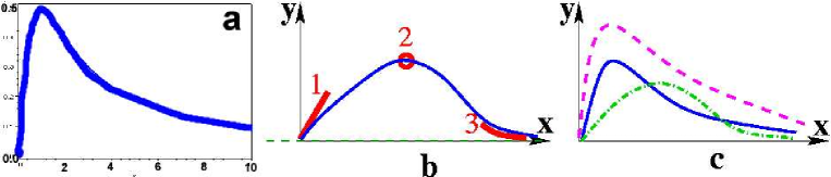
Figure 1.14:

1.4 Implicit function graphs

As we know the relation between two variables $x$ and $y$ can be expressed explicitly in terms of a function $y=f(x)$ that gives us the value of $y$ if we know the value of $x$. It is also possible that the relation between $x$ and $y$ is given implicitly as an equation. Such relations are called implicit functions, and their graphs are implicit function graphs. One of the most effective methods to plot such graphs is to try to solve that implicit equation and rewrite it as one or several explicit functions. In some cases the relations between $x$ and $y$ can be plotted directly. Let us consider two examples:

Example: Draw a graph of the function(s) given by equation: $x^{2}+y^{2}=C^{2}$

Solution: We can either rewrite it as two explicit functions $y=\pm\sqrt{C^{2}-x^{2}}$ and draw the two graphs given by this equation. Alternatively, we can note that $x^{2}+y^{2}$ gives a square of the distance from the point $(0,0)$ to the point $(x,y)$, thus equation $x^{2}+y^{2}=C^{2}$ gives the points located at a distance $C$ from the origin. That is a circle with a radius $C$ with the center at $(0,0)$ (Fig.1.15a). We will use this graph later in our course in chapter 4 to plot fig.4.8a.

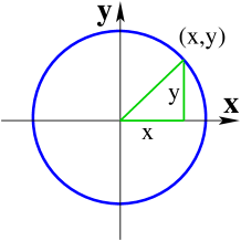
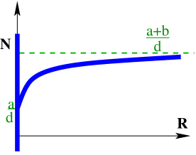
Figure 1.15:

Example: Draw a graph of the function(s) given by equation: $aR+b{R^{2}\over R+c}-dRN=0$, where $R,N\geq 0$ are the variables and $a,b,c,d\geq 0$ are the parameters.

Solution: Let us factor the equation:

$$aR+b{R^{2}\over R+c}-dRN=R(a+b{R\over R+c}-dN)=0$$

The product of two numbers is zero if one of these numbers is zero, therefore this equation is equivalent to:

$$R=0$$

$$or,$$

$$a+b{R\over R+c}-dN=0$$

Graphing of $R=0$ is trivial. In order to graph $a+b{R\over R+c}-dN=0$ let us rewrite it as $dN=a+b{R\over R+c}$, or $N={a\over d}+{{b\over d}R\over R+c}$. The horizontal asymptote of this graph is: $N=\mathop{\lim}\limits_{R\to\infty}{a\over d}+{{b\over d}R\over R+c}={a\over d}+{b/d}={a+b\over d}$. The vertical asymptote occurs if the denominator of the fraction is zero, i.e. at $R=-c$. However, because $R\geq 0$ and $c>0$ this asymptote will be outside the range of our function. Additionally note that this function is similar to the graph of Fig.1.10c, but it is shifted upward by ${a\over d}$. Thus the function graph here contains two branches $R=0$ and $N={a\over d}+{b/dR\over R+c}$ that are plotted in Fig.1.15b

1.5 Exercises

Exercises for section 1.1

1. Perform the indicated operations:

   1. $(ax-2by)*(3y-4bx)+2b*(2ax^{2}+3y^{2})-8xyb^{2}$

   2. ${6\over r}-{5r\over 30r+5}$

2. Find limits:

   1. $\mathop{\lim}\limits_{x\to\infty}{ax+q\over c^{2}+x^{2}}$

   2. $\mathop{\lim}\limits_{N\to\infty}{aN^{2}+q\over{b\over N}+c^{2}+dN^{2}},\;d\neq 0$

3. Solve the equation for the specified variable:

   1. find $r$ in: $3r+2-5(r+1)=6r+4$

   2. find $x$ in: $x+{4\over x}=4$

   3. find $N$ in: $(b-{N\over k})N=0$

   4. find $N$ in: $(b-d(1+{N\over k}))N=0,\;\;d\neq 0;\;k\neq 0$

   5. find $N$ in: $(\frac{b}{1+N/h}-d)N=0,\;b\neq 0;$

4. Solve the system of equations for the specified variables:

   1. find $x,y$ in: $\left\{\begin{array}[]{l}x-2y=-5\\ 2x+y=10\end{array}\right.$

   2. find $x,y$ in: $\left\{\begin{array}[]{l}ax+by=0\\ cx+dy=-b\end{array}\right.$

   3. find $x,y$ in: $\left\{\begin{array}[]{l}x(1-2x)+xy=0\\ 4y-xy=0\end{array}\right.$

   4. find $x,y$ in: $\left\{\begin{array}[]{l}4x-xy-x^{2}=0\\ 9y-3xy-y^{2}=0\end{array}\right.$

   5. find $R,N$ in: $\left\{\begin{array}[]{l}b(1-{R\over k}-d-aN)R=0\\ (R-\delta)N=0\end{array}\right.,\;\;a,b,d,k,\delta\neq 0;$

   Exercises for section 1.2

5. Find the derivative of $f(x)$:

   1. $f(x)={1\over x^{3}}$

   2. $f(x)=e^{-5x};$

   3. $y=(4x-x^{2})*(2x+3)$

   4. $y={x\over a^{2}-x^{2}}$

   Exercises for section 1.3

6. Without plotting the function find the following information about their graph: find the $y$-intercept and zeros; find horizontal or/and vertical asymptotes (if they exist). (Proof of non-existence of asymptotes is not required).

   1. function $y(n)$ given by $y={an^{2}-b\over n^{2}+c^{2}},\;\;a,b,c>0$

   2. function $N(R)$ given by $N={r\over a}(h+R)(1-{R\over K}),\;r,a,h,K\neq 0$

7. Sketch graphs of the following functions:

   1. $y=3-6x$

   2. $y=x-3x^{2}$

   3. $y={3x\over x+a}+4$. Find how the shape of the graph for $x,y\geq 0$ depends on the value of the parameter $a>0$.

   Exercises for section 1.4

8. (a) Sketch qualitative graphs of the following implicit functions. (b) Find how special points of these graphs (intercepts, zeros, asymptotes) depend on parameters. (c) If graph contains several lines find their intersection points. Note, all parameters represent positive numbers.

   1. $x+3y^{2}=0$ on the $xy$ plane

   2. $y^{2}+x^{2}=9$ on the $xy$ plane

   3. $xy=0$ on the $xy$ plane

   4. $dN(a-P)=0$ on the $NP$ plane

   5. $dN+{NP\over N+a}=0$ on the $NP$ plane

   6. $dR(b-R)={cRN\over R+a}$ on the $RN$ plane

   7. $bR(1-{R\over k}-dR)-aNR=0$ on the $RN$ plane

   8. $aN+P(1-eP)+bP=0$ on the $NP$ plane

   Additional exercises

9. Perform the indicated operations:

   1. $((x-2y)*(y-2x)+2y^{2})*{1\over x}$

   2. ${a-2b\over 2p}:{4b-2a\over\sqrt{p}}$

10. Solve the system of equations for the specified variables:

    1. find $A,B,C$ in: $\left\{\begin{array}[]{l}rA(1-{A\over K}-AB)=0\\ AB-dB-BC=0\\ BC-fC=0\end{array}\right.\;\;r,K,d,f>0$

11. Find the derivative of $f(x)$:

    1. $f(x)=2^{x}$

    2. $f(x)=\sqrt{1\over x^{3}}$

    3. $f(g)=cos(x^{2});$

    4. $f=(cos(x))^{2};$

    5. $y=ax*e^{bx}\;a,b>0$

    6. $y={x^{2}-5\over 2x^{2}-3x}$

    7. $y={ax^{2}\over bx-c},\;a,b,c>0$

    8. $y={x\over 1+{x\over d}},\;d>0$

    9. $y={x^{n}\over x^{n}+a^{n}},\;a>0$

12. Solutions of differential equations

    1. Show that function $N(t)=A*e^{3t}$, where $A$ is an arbitrary constant, is a solution of the differential equation: $\frac{dN(t)}{dt}=3N$. For that, compute derivative of this function and substitute this derivative and the function itself to the equation and show that the left hand side of the equation equals to the right hand side.

    2. Show, using the same steps that the function $N(t)=s(1-e^{t})+Ae^{-t}$, where $a$ is an arbitrary constant and $s$ is a parameters, is a solution of the differential equation $\frac{dN(t)}{dt}=s-N$

13. Assume that $x(t)$ is an unknown function of $t$. For $f(x)$ listed below find the following derivatives: ${df\over dx}$ and ${df\over dt}$.

    1. $f(x)=x^{3}$

    2. $f(x)=e^{-ax}$

    3. Find the expression for ${df\over dt}$ for an arbitrary $f(x(t))$.

14. Without plotting the function find the following information about their graph: find the $y$-intercept and zeros; find horizontal or/and vertical asymptotes (if they exist).

    1. function $y(x)$ given by $y={x-4\over x^{2}-3x+2}$

    2. function $y(x)$ given by $y=a:{b\over x^{3}-c}\;\;a,b,c>0$

15. Sketch graphs of the following functions:

    1. $x=4e^{-3t}$

    2. $y=x^{2}+2x-3$

    3. $y={2\over x+3}$

    4. $y={bx^{2}\over x^{2}+a^{2}}+4$. Find how the shape of the graph depends on the value of the parameters $a>0$ and $b>0$.

    5. $y={bx^{2}\over x^{3}+c^{3}}$, Find how the shape of the graph depends on the value of the parameter $c>0$ and $b>0$.

    6. $f(n)=rn*(1-{n\over k})-h$, $k\neq 0$ find for which values of the parameter $h>0$ the graph touches the $n$-axis. Tip: draw graph for $h=0$ and think about how $h$ affects this graph.

16. Sketch qualitative graphs of the following pairs of implicit functions on the same graph. Find all intersection points.

    1. $aN-P(1+eP)-bP=0\quad and\quad bP-cN=0\quad parameters\;\;a,b,c,e>0$

    2. $rR(1-R/K)-\frac{NR}{h+R}=0\quad and\quad\frac{NR}{h+R}-dN=0\quad parameters\;\;r,K,h,d>0$

Chapter 2 Selected topics of calculus

In this chapter we introduce several new notions on calculus and algebra which are important for our course.

2.1 Complex numbers

Complex numbers were introduced for the solution of algebraic equations. It turns out that in many cases we can not find the solution of even very simple quadratic equations. Consider the general quadratic equation:

$${\lambda}^{2}+B\lambda+C=0$$ (2.1)

The roots of (2.1) are given by the well known ’abc’ formula:

$$\lambda_{12}={-B\pm\sqrt{B^{2}-4C}\over 2}={-B\pm\sqrt{D}\over 2}$$ (2.2)

where

$$D=B^{2}-4C$$ (2.3)

What happens with this equation if $D<0$? Does the equation have roots in this case?

Complex numbers help to solve such kind of problems. The first step is to consider the equation

$$\lambda^{2}=-1$$ (2.4)

Let us claim that (2.4) has a solution and denote it in the following way:

$$\lambda_{12}=\pm i$$ (2.5)

where

$$i=\sqrt{-1}$$ (2.6)

Here $i$ is the basic complex number which is similar to ${}^{\prime}1^{\prime}$ for real numbers. Using it we can denote solutions of other similar equations. For example if

$$\lambda^{2}=-4,\;\lambda=\sqrt{-1*4}=\sqrt{-1}\sqrt{4}=i*(\pm 2)=\pm 2i.$$

Similarly the equation $\lambda^{2}=-a^{2}$, has solutions $\lambda=\pm ai$. Although we call $ai$ a complex number, it is quite different from usual real numbers. Using complex numbers $ai$ we cannot count how many books we have in the library, for example. The only meaning of $i$ is that $i^{2}=-1$, and $ai$ is just a designation of a root of the equation $\lambda^{2}=-a^{2}$.

Now we can solve equation (2.1) for the case $D<0$. If $D<0$, then $\sqrt{D}=i\sqrt{-D}$ and

$$\lambda_{12}={-B\pm i\sqrt{-D}\over 2}$$ (2.7)

Example. Solve the equation $\lambda^{2}+2\lambda+10=0$

Solution.

$$\lambda_{12}={-2\pm\sqrt{4-4*10}\over 2}={-2\pm\sqrt{-36}\over 2}={-2\pm 6i\over 2},$$ (2.8)

or $\lambda_{1}=-1+3i,\;\;\;\lambda_{2}=-1-3i.$

We see, that solution of this equation $\lambda_{1,2}$ has two parts, one part is just a real number ’-1’, which is the same for $\lambda_{1}$ and $\lambda_{2}$ and the other part, is $i$ times another real number ’3’ which has opposite signs for $\lambda_{1}$ and $\lambda_{2}$. This is a general form of representation of complex number. Any complex number can be represented in the form:

$$z=\alpha+i\beta$$ (2.9)

where $\alpha$ is called the real part of the complex number $z$, and $\beta$ is called the imaginary part of $z$. The notation for the real part is $Rez$ and for the imaginary part is $Imz$. In our example $Re\lambda_{1}=-1;Im\lambda_{1}=3.$ and $Re\lambda_{2}=-1;Im\lambda_{2}=-3.$

We can work with complex numbers in the same way as with usual real numbers and expressions. The only thing which we need to remember, is that $i^{2}=-1$.

To add two complex numbers we need to add their real and imaginary parts. For example

$$z_{1}=3+10i,z_{2}=-5+4i,\;\;z_{1}+z_{2}=(3+10i)+(-5+4i)=3+10i+-5+4i=-2+14i.$$

Similarly, multiplication by a real number results in multiplication of the real and imaginary part by this number

$$z_{1}=3+10i;\;10z_{1}=10*(3+10i)=30+100i.$$

Multiplication of two complex numbers is just an exercise in multiplication of two expressions $z_{1}=3+10i,z_{2}=-5+4i;\;z_{1}*z_{2}=(3+10i)*(-5+4i)=3*(-5)+3*4i+10i*(-5)+10i*4i=-15+12i-50i+40i^{2}=-15-38i-40\;(as\;i^{2}=-1)=-55-38i.$

Similarly

$$(z_{1})^{2}=(3+10i)^{2}=3^{2}+2*3*10i+(10i)^{2}=9+60i+100i^{2}=9+60i-100=-91+60i.$$

Now we can check that $\lambda_{1}=-1+3i$ is a solution of the equation in example (2.8). In fact: $\lambda^{2}+2\lambda+10=(-1+3i)^{2}+2*(-1+3i)+10=(-1)^{2}+2*(-1)*3i+(3i)^{2}-2+6i+10=1-6i-9-2+6i+10=(1-9-2+10)-6i+6i=0-0i=0$, i.e. left hand side of this equation after substitution of $\lambda_{1}=-1+3i$ equals zero and thus $\lambda_{1}=-1+3i$ is the root of this equation.

One more definition. The number $z_{2}=a-ib$ is called the complex conjugate to the number $z_{1}=a+ib$ and is denoted as $\bar{z}_{1}=z_{2}=a-ib$. Complex conjugate numbers have the same real parts, but their imaginary parts have opposite signs.

Roots of a quadratic equation with negative discriminant $D<0$ are complex conjugate to each other. It follows from the formula (2.7)

$$\lambda_{1}={-B+i\sqrt{-D}\over 2}\quad\lambda_{2}={-B-i\sqrt{-D}\over 2}$$ (2.10)

hence:

$$Re\lambda_{1}=Re\lambda_{2}={-B\over 2};\quad Im\lambda_{1}={\sqrt{-D}\over 2};\quad Im\lambda_{2}=-{\sqrt{-D}\over 2}.$$ (2.11)

Finally consider two more basic operations. If $z=a+ib$, then, $|z|=\sqrt{a^{2}+b^{2}}$ is called the absolute value, or modulus of $z$. Note, that ${|z|}^{2}=z\bar{z}$, as $(a+ib)*(a-ib)=a^{2}-(ib)^{2}=a^{2}+b^{2}$.

We use this trick to introduce division of two complex numbers

$${z_{1}\over z_{2}}={z_{1}\bar{z_{2}}\over z_{2}\bar{z_{2}}}$$

So, to divide two complex numbers we multiply the numerator and the denominator by a number which is the complex conjugate to the denominator, and we get the answer in the usual form.

Example

$${1+3i\over 1-4i}={1+3i\over 1-4i}*{1+4i\over 1+4i}={(1+3i)(1+4i)\over 1^{2}+4^{2}}={1+3i+4i+12i^{2}\over 17}={-11+7i\over 17}={-11\over 17}+{7\over 17}i\;$$

2.2 Matrices

From a very general point of view a matrix is a representation of data in the form of a rectangular table. An example of a matrix composed of numbers is given below:

$$A=\left(\begin{array}[]{lcr}1&4&5\\ 2&6&10\end{array}\right)$$ (2.12)

This matrix $A$ has two rows and three columns. We will call this a matrix of the size $2\times 3$. In general matrix size is defined as $number\;of\;rows\times number\;of\;columns$. Even if you did not have matrix algebra in school, you probably know at least one matrix object, that is a vector. Indeed, a vector is an object which is characterized by its components: two numbers in two dimensions or three numbers in three dimensions. In matrix algebra vectors can be represented in two forms: as a column vector, i.e. as $n\times 1$ matrix (preferred representation), or as a row vector, i.e. as $1\times n$ matrix. For example a vector $V$ with the $x$-component $V_{x}=2$ and the $y$-component $V_{y}=1$ can be represented a column or as a row vector as:

$$\vec{V}=\left(\begin{array}[]{c}2\\ 1\end{array}\right)\hskip 36.0ptor\hskip 36.0pt\vec{V}=\left(\begin{array}[]{lr}2&1\end{array}\right)$$

Using matrices we can perform the same operations on large blocks of data simultaneously. For example, if we need to multiply all 6 numbers of matrix $A$ in (2.12) by $4$, we can write it as $4A$ which will mean:

$$4A=4*\left(\begin{array}[]{lcr}1&4&5\\ 2&6&10\end{array}\right)=\left(\begin{array}[]{lcr}4*1&4*4&4*5\\ 4*2&4*6&4*10\end{array}\right)=\left(\begin{array}[]{lcr}4&16&20\\ 8&24&40\end{array}\right)$$ (2.13)

This operation is called multiplication of a matrix by a number. For a general $2\times 2$ matrix this can be written as:

$$\lambda\left(\begin{array}[]{lr}a&b\\ c&d\end{array}\right)=\left(\begin{array}[]{lr}\lambda a&\lambda b\\ \lambda c&\lambda d\end{array}\right)$$

Similarly, addition of matrices is adding the numbers that have the same location. This operation is defined only for two matrices of the same size:

$$A+B=\left(\begin{array}[]{lcr}1&4&5\\ 2&6&10\end{array}\right)+\left(\begin{array}[]{lcr}2&1&4\\ 1&3&5\end{array}\right)=\left(\begin{array}[]{lcr}1+2&4+1&5+1\\ 2+1&6+3&10+5\end{array}\right)=\left(\begin{array}[]{lcr}3&5&6\\ 3&9&15\end{array}\right)$$ (2.14)

For general $2\times 2$ matrices it can be written as:

$$\left(\begin{array}[]{lr}a&b\\ c&d\end{array}\right)+\left(\begin{array}[]{lr}x&y\\ z&w\end{array}\right)=\left(\begin{array}[]{lr}a+x&b+y\\ c+z&d+w\end{array}\right)$$ (2.15)

Multiplication of matrices is not so trivial. In general matrix multiplication is defined as the products of the rows of the first matrix with the columns of the second matrix. Thus, to fund the element in row $i$ and column $j$ of the resulting matrix we need to multiply the $i$th row of the first matrix by the $j$th column of the second matrix. Thus we can multiply two matrices $A*B$ only if the number of columns in matrix $A$ equals the number of rows in matrix $B$.

For a product of two $2\times 2$ matrices this gives:

$$\left(\begin{array}[]{lr}a&b\\ c&d\end{array}\right)\left(\begin{array}[]{lr}x&y\\ z&w\end{array}\right)=\left(\begin{array}[]{lr}ax+bz&ay+bw\\ cx+dz&cy+dw\end{array}\right)$$ (2.16)

From this it follows that multiplication of a matrix by a column vector is given by:

$$\left(\begin{array}[]{lr}a&b\\ c&d\end{array}\right)\left(\begin{array}[]{c}v_{x}\\ v_{y}\end{array}\right)=\left(\begin{array}[]{c}av_{x}+bv_{y}\\ cv_{x}+dv_{y}\end{array}\right)$$ (2.17)

The last equation is useful for representation of linear systems as can be seen from the following example. Assume we have a system of linear equations:

$$\left\{\begin{array}[]{l}x-2y=-5\\ 2x+y=10\end{array}\right.$$ (2.18)

we can write the coefficients at $x$ and $y$ in the left hand side as a square matrix:

$$A=\left(\begin{array}[]{lr}1&-2\\ 2&1\end{array}\right).$$

We also have two numbers in the right hand side which we can write as a column vector:

$$\vec{V}=\left(\begin{array}[]{c}-5\\ 10\end{array}\right).$$

Now if we write $x$ and $y$ as a column vector:

$$\vec{X}=\left(\begin{array}[]{c}x\\ y\end{array}\right).$$

we can represent system (2.18) using matrix multiplication (2.17) as:

$$A\vec{X}=\vec{V};\;\;or\;\;\left(\begin{array}[]{lr}1&-2\\ 2&1\end{array}\right)\left(\begin{array}[]{c}x\\ y\end{array}\right)=\left(\begin{array}[]{c}-5\\ 10\end{array}\right)$$ (2.19)

Indeed, from (2.17) we get $\left(\begin{array}[]{lr}1&-2\\ 2&1\end{array}\right)\left(\begin{array}[]{c}x\\ y\end{array}\right)=\left(\begin{array}[]{c}1*x-2*y\\ 2*x+1*y\end{array}\right)$, that proves this result.

Another important matrix operation is the determinant of a square 2x2 matrix, which for the matrix $A=\left(\begin{array}[]{lr}a&b\\ c&d\end{array}\right)$ is defined as:

$$det\left|\begin{array}[]{lr}a&b\\ c&d\end{array}\right|=ad-cb$$ (2.20)

The determinant of a matrix has many important applications in algebra. For example using determinants it is possible to find solution of system of linear equations (e.g. system (2.18)) in the form of so-called Cramer’s rule, which was published by Gabriel Cramer as early as in mid-18th century. Cramer’s rule is briefly formulated in exercise 7 at the end of this chapter.

Now let us consider one of the most important problems in matrix algebra: the eigen value problem.

2.3 Eigenvalues and eigenvectors

Let us start with a definition:

Definition 1

A nonzero vector $\mathbf{v}$ and number $\lambda$ are called an eigen vector and an eigen value of a square matrix $A$ if they satisfy equation:

$$A\mathbf{v}=\lambda\mathbf{v}$$ (2.21)

Eigen vectors are not unique, and it is easy to see that if we multiply it by an arbitrary constant $k$ we get another eigen vector corresponding to the same eigen value. Indeed by multiplying (2.21) by $k$ we get:

$$kA\mathbf{v}=k\lambda\mathbf{v}\quad or\quad A(k\mathbf{v})=\lambda(k\mathbf{v})$$ (2.22)

therefore, we can say that $k\mathbf{v}$ is also an eigen vector of (2.21) corresponding to eigen value $\lambda$.

For example, for matrix $A=\left(\begin{array}[]{lr}1&2\\ 2&1\end{array}\right)$, number $\lambda=3$ and vector $\mathbf{v}=\left(\begin{array}[]{c}1\\ 1\end{array}\right)$ are an eigen value and eigen vector as:

$$A\mathbf{v}=\left(\begin{array}[]{lr}1&2\\ 2&1\end{array}\right)\left(\begin{array}[]{c}1\\ 1\end{array}\right)=\left(\begin{array}[]{c}1*1+2*1\\ 2*1+1*1\end{array}\right)=\left(\begin{array}[]{c}3\\ 3\end{array}\right)=3\left(\begin{array}[]{c}1\\ 1\end{array}\right)=3\mathbf{v}$$ (2.23)

If we multiply $\mathbf{v}=\left(\begin{array}[]{c}1\\ 1\end{array}\right)$ by any number, e.g. $2$, $25$, or etc., we will get new eigen vectors $\mathbf{v}=\left(\begin{array}[]{c}2\\ 2\end{array}\right)$, $\mathbf{v}=\left(\begin{array}[]{c}25\\ 25\end{array}\right)$ of this matrix for $\lambda=3$. You can check it in the same way as we did in (2.23) for a vector $\mathbf{v}=\left(\begin{array}[]{c}1\\ 1\end{array}\right)$.

Finding eigen values and eigen vectors is one of the most important problems in applied mathematics. It arises in many biological applications, such as population dynamics, biostatistics, bioinformatics, image processing and many others. In our course we will apply it for the solution of systems of differential equations, which we will consider in chapter 4.

Let us consider how to solve the eigen value problem for a 2x2 matrix $A=\left(\begin{array}[]{lr}a&b\\ c&d\end{array}\right)$. For that we need to find $\lambda$ and $\left(\begin{array}[]{c}v_{x}\\ v_{y}\end{array}\right)$ satisfying:

$$A\mathbf{v}=\left(\begin{array}[]{lr}a&b\\ c&d\end{array}\right)\left(\begin{array}[]{c}v_{x}\\ v_{y}\end{array}\right)=\lambda\left(\begin{array}[]{c}v_{x}\\ v_{y}\end{array}\right).$$ (2.24)

We can rewrite it as a system of two equations with three unknowns $\lambda,v_{x},v_{y}$:

$$\left\{\begin{array}[]{l}a*v_{x}+b*v_{y}=\lambda v_{x}\\ c*v_{x}+d*v_{y}=\lambda v_{y}\end{array}\right.$$ (2.25)

If we collect all unknowns at the left hand side we will get the following system:

$$\left\{\begin{array}[]{l}(a-\lambda)*v_{x}+b*v_{y}=0\\ c*v_{x}+(d-\lambda)*v_{y}=0\end{array}\right.\quad or\;in\;matrix\;form\;\left(\begin{array}[]{lr}a-\lambda&b\\ c&d-\lambda\end{array}\right)\left(\begin{array}[]{c}v_{x}\\ v_{y}\end{array}\right)=\left(\begin{array}[]{c}0\\ 0\end{array}\right).$$ (2.26)

This system always has a solution $v_{x}=v_{y}=0$, however it is not an eigen vector, as in accordance with the definition the eigen vector should be nonzero. In order to find non-zero solutions let us multiply the first equation by $d-\lambda$, the second equation by $b$ and subtract them. Multiplication gives:

$$\left\{\begin{array}[]{l}(d-\lambda)*[(a-\lambda)*v_{x}+b*v_{y}]=0\\ b*[c*v_{x}+(d-\lambda)*v_{y}]=0\end{array}\right.$$ (2.27)

Subtraction of the equations results in:

$$\begin{array}[]{l}(d-\lambda)*(a-\lambda)*v_{x}+(d-\lambda)*b*v_{y}=0\\ -\\ b*c*v_{x}+b*(d-\lambda)*v_{y}=0\\ gives\\ (d-\lambda)*(a-\lambda)*v_{x}-b*c*v_{x}+(d-\lambda)*b*v_{y}-b*(d-\lambda)*v_{y}=0\\ or\end{array}$$

$$[(d-\lambda)*(a-\lambda)-b*c]*v_{x}=0$$ (2.28)

as $v_{x}\neq 0$ we get:

$$(d-\lambda)*(a-\lambda)-b*c=\lambda^{2}-(a+d)\lambda+(ad-cb)=0$$ (2.29)

This is a quadratic equation with unknown $\lambda$ and for each particular coefficients $a,b,c,d$ we can find two solutions: $\lambda_{1}$ and $\lambda_{2}$ using the ’abc’ formula. Thus we found that the eigenvalue problem for a $2x2$ matrix (2.24) has solutions for the eigen values $\lambda$. In general, for a $nxn$ matrix that the eigen value problem has $n$ solutions for $\lambda$.

Equation (2.29) is very important in our course and it has a special name: characteristic equation. In most of the courses on mathematics this equation, however, is written in a slightly different matrix form. To derive it let us recall the definition of the determinant of a matrix given in section 2.2:
$det\left|\begin{array}[]{lr}a&b\\ c&d\end{array}\right|=ad-cb.$ Similarly the determinant of matrix $\left(\begin{array}[]{lr}a-\lambda&b\\ c&d-\lambda\end{array}\right)$ is:

$$det\left|\begin{array}[]{lr}a-\lambda&b\\ c&d-\lambda\end{array}\right|=(a-\lambda)(d-\lambda)-bc$$ (2.30)

which coincides with the left hand side of characteristic equation (2.29) and thus the characteristic equation can be rewritten as:

$$det\left|\begin{array}[]{lr}a-\lambda&b\\ c&d-\lambda\end{array}\right|=0$$ (2.31)

Let us use this approach to find the eigen values of matrix $A$ from example (2.23). We get the following characteristic equation:

$$\begin{array}[]{l}Det\left|\begin{array}[]{lr}1-\lambda&2\\ 2&1-\lambda\end{array}\right|=(1-\lambda)(1-\lambda)-2*2\\ =1-\lambda-\lambda+\lambda^{2}-4=\lambda^{2}-2\lambda-3=0\end{array}$$

From the ’abc’ formula:

$$\lambda_{1,2}={2\pm\sqrt{4+12}\over 2}={2\pm\sqrt{16}\over 2};\qquad\lambda_{1}=3\quad\lambda_{2}=-1$$

therefore we found two eigen values $\lambda_{1}=3$ and $\lambda_{2}=-1$.

Now, let us find eigen vectors. For that let us substitute the found eigen values to the original equation (2.26) and solve it for $v_{x}$ and $v_{y}$. Let us do it first for a particular example (2.23) for which we have found eigen values $\lambda_{1}=3$ and $\lambda_{2}=-1$. For eigen vector corresponding to eigen value $\lambda_{1}=3$ we obtain:

$$\left\{\begin{array}[]{l}(1-3)v_{x}+2v_{y}=0\\ 2v_{x}+(1-3)v_{y}=0\end{array}\right.\quad or\quad\left\{\begin{array}[]{l}-2v_{x}+2v_{y}=0\\ 2v_{x}-2v_{y}=0\end{array}\right.\quad or\quad\left\{\begin{array}[]{l}-2v_{x}=-2v_{y}\\ 2v_{x}=2v_{y}\end{array}\right.$$ (2.32)

Both equations give the same solution $v_{x}=v_{y}$. This means that if $v_{y}=1$, then $v_{x}=1$ and a pair $\left(\begin{array}[]{c}1\\ 1\end{array}\right)$ satisfies the system and thus gives an eigen vector of problem (2.23). We can also use any other value for $v_{y}$. For example, if we use $v_{y}=2$ then $v_{x}$ will be $v_{x}=2$ and we get another eigen vector $\left(\begin{array}[]{c}2\\ 2\end{array}\right)$, etc. In general any $v_{x}=k$, and $v_{y}=k$ give an eigen vector. We can express it by the following formula:

$$\left(\begin{array}[]{c}v_{x}\\ v_{y}\end{array}\right)=k\left(\begin{array}[]{c}1\\ 1\end{array}\right)$$ (2.33)

where $k$ is an arbitrary number. Formula (2.33) gives all possible solutions of eq.(2.32). It also illustrates a general property of eigen vectors which we have proven in (2.22), that if we multiply an eigen vector by an arbitrary number $k$ will get also an eigen vector of our matrix. Using this property we can formulate an easy way to write a formula for all eigen vectors. For that we take any found eigen vector and multiply it by an arbitrary number $k$. Note, that if for problem (2.32) we use another found eigen vector $\left(\begin{array}[]{c}2\\ 2\end{array}\right)$, we can write an answer as $\left(\begin{array}[]{c}v_{x}\\ v_{y}\end{array}\right)=k\left(\begin{array}[]{c}2\\ 2\end{array}\right)$. At the first glance this formula is different from (2.33). However, it is easy to see that both formulas give the same result: this is because $k$ in (2.33) is an arbitrary constant and any vector given by the formula (2.33) with $\left(\begin{array}[]{c}1\\ 1\end{array}\right)$ can be obtained using the formula $k\left(\begin{array}[]{c}2\\ 2\end{array}\right)$ for another value of $k$. Thus the answer to our problem: to find eigen vectors of matrix (2.23) for eigen value $\lambda_{1}=3$, can be written as $\left(\begin{array}[]{c}v_{x}\\ v_{y}\end{array}\right)=\left(\begin{array}[]{c}1\\ 1\end{array}\right)$, or $\left(\begin{array}[]{c}v_{x}\\ v_{y}\end{array}\right)=\left(\begin{array}[]{c}2\\ 2\end{array}\right)$, or etc. These vectors give particular solutions of this problem. We can also write a formula for all solutions as $\left(\begin{array}[]{c}v_{x}\\ v_{y}\end{array}\right)=k\left(\begin{array}[]{c}1\\ 1\end{array}\right)$, or $\left(\begin{array}[]{c}v_{x}\\ v_{y}\end{array}\right)=k\left(\begin{array}[]{c}2\\ 2\end{array}\right)$, or etc. As we discussed above all these answers will be correct and equivalent.

Similarly we find the eigen vector corresponding to the other eigen value $\lambda_{2}=-1$:

1. Substitution:

   $$\left\{\begin{array}[]{l}(1-(-1))v_{x}+2v_{y}=0\\ 2v_{x}+(1-(-1))v_{y}=0\end{array}\right.\quad or\quad\left\{\begin{array}[]{l}2v_{x}+2v_{y}=0\\ 2v_{x}+2v_{y}=0\end{array}\right.\quad or\quad\left\{\begin{array}[]{l}2v_{x}=-2v_{y}\\ 2v_{x}=-2v_{y}\end{array}\right.$$ (2.34)

2. Relation between $v_{x}$ and $v_{y}$:

   $$v_{x}=-v_{y}$$

3. Eigen vector: use e.g. $v_{y}=1$, thus $v_{x}=-1$

   $$\mathbf{v}=\left(\begin{array}[]{c}-1\\ 1\end{array}\right)$$

   The general form is $\mathbf{v}=k\left(\begin{array}[]{c}-1\\ 1\end{array}\right)$, where $k$ is an arbitrary number.

Note, that in both cases in order to find eigen vectors we could use the first equation only (see equations (2.32) and (2.34)), and the second equation in both cases did not provide us any new information. It is not a coincidence, and this property is the basis for the following express method for finding eigen vectors:

Express method for finding eigen vectors

Let us derive a formula for finding the eigen vectors of a general system (2.25). We assume that we have found eigen values $\lambda_{1}$ and $\lambda_{2}$ from the characteristic equation (2.31). To find the corresponding eigen vectors we need to substitute the found eigen values into the matrix and solve the following system of linear equations (2.26):

$$\left\{\begin{array}[]{l}(a-\lambda_{1})v_{x}+bv_{y}=0\\ cv_{x}+(d-\lambda_{1})v_{y}=0\end{array}\right.\\$$ (2.35)

It is easy to check that if we use for $v_{x}$ and $v_{y}$ the values $v_{x}=-b$ and $v_{y}=a-\lambda_{1}$ it gives the solution of the first equation:

$$(a-\lambda_{1})v_{x}+bv_{y}=(a-\lambda_{1})(-b)+b(a-\lambda_{1})=-b(a-\lambda_{1})+b(a-\lambda_{1})=0$$

If we substitute these expressions into the second equation we get:

$$cv_{x}+(d-\lambda_{1})v_{y}=-cb+(d-\lambda_{1})(a-\lambda_{1})=0$$

To prove that this expression is also zero, note that $(d-\lambda_{1})(a-\lambda_{1})-cb$ is zero in accordance with the characteristic equation (2.29). Therefore $v_{x}=-b$ and $v_{y}=a-\lambda_{1}$ give a solution of (2.35) which is an eigen vector corresponding to the eigen value $\lambda_{1}$. Similarly we find the eigen vector corresponding to the the eigen value $\lambda_{2}$.

However, this approach does not work if in (2.26) both $b=0$ and $a-\lambda=0$. In this case we can use the second equation $cv_{x}+(d-\lambda_{1})v_{y}=0$ and find an eigen vector as $v_{x}=d-\lambda_{1}$ and $v_{y}=-c$. Indeed:

$$cv_{x}+(d-\lambda_{1})v_{y}=c(d-\lambda_{1})+(d-\lambda_{1})(-c)=0$$

As in the previous case it is easy to show that this vector satisfies the other (first) equation as: $(a-\lambda_{1})v_{x}+bv_{y}=(a-\lambda_{1})(d-\lambda_{1})+b(-c)=0$ due to (2.35).

The final formulas are:

$${\bf v_{1}}=\left(\begin{array}[]{c}v_{1x}\\ v_{1y}\end{array}\right)=\left(\begin{array}[]{c}-b\\ a-\lambda_{1}\end{array}\right)\quad{\bf v_{2}}=\left(\begin{array}[]{c}v_{2x}\\ v_{2y}\end{array}\right)=\left(\begin{array}[]{c}-b\\ a-\lambda_{2}\end{array}\right)$$ (2.36)

or

$${\bf v_{1}}=\left(\begin{array}[]{c}v_{1x}\\ v_{1y}\end{array}\right)=\left(\begin{array}[]{c}d-\lambda_{1}\\ -c\end{array}\right)\quad{\bf v_{2}}=\left(\begin{array}[]{c}v_{2x}\\ v_{2y}\end{array}\right)=\left(\begin{array}[]{c}d-\lambda_{2}\\ -c\end{array}\right)$$ (2.37)

where $a,b$ are the elements of the matrix $A=\left(\begin{array}[]{lr}a&b\\ c&d\end{array}\right)$.

Either (2.36) or (2.37) can be used to find eigen vectors. (Both answers will be valid.) If, however, one of the formulas gives a zero eigen vector, we should use the other one to obtain a non-zero vector.

Let us apply these formulas for the system (2.23) with matrix $A=\left(\begin{array}[]{lr}1&2\\ 2&1\end{array}\right)$ and eigen values $\lambda_{1}=3;\lambda_{2}=-1$. The eigen vectors can be found from (2.36) as:

$$\lambda_{1}=3;\left(\begin{array}[]{c}v_{1x}\\ v_{1y}\end{array}\right)=\left(\begin{array}[]{c}-2\\ 1-(3)\end{array}\right)=\left(\begin{array}[]{c}-2\\ -2\end{array}\right)\quad\lambda_{2}=-1;\left(\begin{array}[]{c}v_{2x}\\ v_{2y}\end{array}\right)=\left(\begin{array}[]{c}-2\\ 1-(-1)\end{array}\right))=\left(\begin{array}[]{c}-2\\ 2\end{array}\right)$$ (2.38)

and from (2.37) as:

$$\lambda_{1}=3;\left(\begin{array}[]{c}v_{1x}\\ v_{1y}\end{array}\right)=\left(\begin{array}[]{c}1-3\\ -2)\end{array}\right)=\left(\begin{array}[]{c}-2\\ -2\end{array}\right)\quad\lambda_{2}=-1;\left(\begin{array}[]{c}v_{2x}\\ v_{2y}\end{array}\right)=\left(\begin{array}[]{c}1-(-1)\\ -2\end{array}\right))=\left(\begin{array}[]{c}2\\ -2\end{array}\right)$$ (2.39)

We see that the vectors differ from the vectors found earlier, but it is easy to find that they are equivalent. For example, if we multiply the first vector by $-{1\over 2}$ we find $-{1\over 2}\left(\begin{array}[]{c}-2\\ -2\end{array}\right)=\left(\begin{array}[]{c}1\\ 1\end{array}\right)$, thus the same vector which we found earlier in (2.33). We also see that formulas (2.38) and (2.39) give equivalent result. Indeed, first vectors obtained form (2.38) and (2.39) are the same. For second vectors note that: $-1\left(\begin{array}[]{c}-2\\ 2\end{array}\right)=\left(\begin{array}[]{c}2\\ -2\end{array}\right).$

2.4 Functions of two variables

A function of two variables $f(x,y)$ describes the rule of finding the value of function $f$, if we know the values of the variables $x$ and $y$. For example, the area of a right-angled triangle with the sides $x$, and $y$ is given by the following function of two variables: $f(x,y)=xy/2$. Another example is the rate of growth of a prey population in a typical ecological predator-prey model: $f(x,y)=3x-3x^{2}-1.5xy$, where $x$ is the prey population and $y$ is the predator population. The graph of the function of one variable $y=f(x)$ is a line on the $Oxy$-plane. To sketch the graph of the function of two variables $f(x,y)$, we must use a three dimensional space $(x,y,z)$: the $Oxy$-plane for the values of the independent ’ input’ variables $x,y$, and the third axis $z$ for the function ’output’ value $z=f(x,y)$. In such a representation the graph will be a surface in a three dimensional space. Fig.2.1 shows a graph of the function $f(x,y)=3x-3x^{2}-1.5xy$ plotted by a computer.

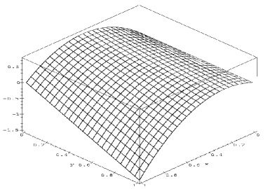
Figure 2.1:

Derivatives. The next step is the definition of the derivative of $f(x,y)$. The main idea of finding the derivative of $f(x,y)$ is to fix one variable at a constant value, say $x=x^{*}$. After that we will get a function of one variable $y$ only ($f(x^{*},y)$). Now, we can find the derivative of $f(x^{*},y)$, as the usual derivative of a function of one variable $y$. For example, $f(x,y)=3x-3x^{2}-1.5xy$. Let us fix $x=x^{*}=2$. We get the following function of one variable: $f(2,y)=3*2-3*2^{2}-1.5*2y=-6-3y$. We can easily find the derivative now: $df(2,y)/dy=d(-6-3y)/dy=-3$.

This type of derivative is called the partial derivative of $f(x,y)$ with respect to $y$ at $x=2$. We denote it as

$$\partial f/\partial y|_{x=2}=-3$$

We can find such a derivative at $x=3$, or at any other value of $x$. In fact for an arbitrary $x=x^{*}$, $f(x^{*},y)=3*x^{*}-3*{x^{*}}^{2}-1.5*x^{*}*y$, and

$$\partial f/\partial y|_{x=x^{*}}=\partial(3*x^{*}-3*{x^{*}}^{2}-1.5*x^{*}*y)/\partial y=0-0-1.5*x^{*}$$

Here $\partial(3*x^{*})/\partial y=0$ as we replaced $x$ by a constant $x^{*}$ and the derivative of a constant is zero. Similarly, $\partial(-3*{x^{*}}^{2})/\partial y=0$, and $\partial(-1.5*x^{*}*y)/\partial y=-1.5*x^{*}$, as $-1.5*x^{*}$ is a constant and the derivative of $(ky)^{\prime}=k$. It is generally accepted to make all these differentiations without explicitly replacing $x$ by $x^{*}$. We just should keep in mind, that for such a differentiation we treat $x$ as a constant. Thus, to find the derivative of $f$ with respect to $y$ we just write:

$$\partial f/\partial y=\partial(3x-3{x}^{2}-1.5xy)/\partial y=-1.5x.$$

keeping in mind that $x$ is considered as a constant and not a variable during this differentiation.

This expression is called the partial derivative of $f(x,y)$ with respect to $y$ and is denoted as $\partial f/\partial y$.

Similarly, we can introduce a partial derivative of $f$ with respect to $x$: $\partial f/\partial x$. To compute it, we fix $y$ (treat $y$ as a constant) and make the usual differentiations with respect to $x$. In our example it gives:

$$\partial f/\partial x=\partial(3x-3{x}^{2}-1.5xy)/\partial x=3-3*2x-1.5y$$

Here $\partial(3x)/\partial x=3$, $\partial(-3x^{2})/\partial x=-3*2x$, and $\partial(-1.5xy)/\partial x=-1.5y$ as $y$ is fixed.

Example. Find $\partial z/\partial x$ and $\partial z/\partial y$ for $z=y^{3}\sin x$

Solution $\partial z/\partial x=y^{3}\cos x$, as for $\partial/\partial x$ we fix $y$, and $\partial(\sin x)/\partial x=\cos x$. Similarly, $\partial z/\partial y=\partial(y^{3}\sin x)/\partial y=3y^{2}\sin x$, as $x$ and hence $\sin x$ is treated as a constant.

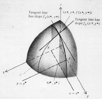
Figure 2.2:

The geometrical representation of a partial derivative is clear from fig.2.2. To compute $\partial f/\partial x$ we fix $y$, i.e. assume that $y$ has some value $y=y^{*}$. The condition $y=y^{*}$ geometrically gives a horizontal line on the $Oxy$ plane fig.2.2a, or a line parallel to the $x$-axis. In 3D this line gives a curve on the 3D surface in graph fig.2.2b, which is a 1D function. The partial derivative with respect to $x$ for this particular $y^{*}$ will give us the slope of the tangent line to this 1D function. Thus (see fig.2.2) $\partial f/\partial x$ gives the slope of the tangent line in the direction of the $x$-axis or the rate of change of $f(x,y)$ in the $x$ direction. Similarly, computing $\partial f/\partial y$ we fix $x$, i.e. assume that $x$ has some value $x=x^{*}$. It gives us a vertical line on the $Oxy$ plane fig.2.2a, or a line parallel to the $y$-axis. Thus $\partial f/\partial y$ gives the slope of the tangent line in the direction of the $y$-axis, or the rate of change of $f(x,y)$ in the $y$ direction. If we consider $f(x,y)$ as a mountain $\partial f/\partial x$ gives the slope of the mountain if we climb in the $x$-direction and $\partial f/\partial y$ gives the slope of the mountain if we climb in the $y$-direction.

Note, that in general at each point on a surface we can draw a tangent line in any direction, and partial derivatives $\partial f/\partial x$ and $\partial f/\partial y$ give the slopes of two of these possible tangent lines. Note, that the slope of a tangent line any direction can be obtained as a combination of these two slopes.

Linear approximation Let us derive a formula for approximating a functions of two variables $f(x,y)$. Let us assume that we know $f(x,y)$ and its partial derivatives at some point $x^{*},y^{*}$ and that we want to find the value of a function at the close point $x,y$ (fig.2.3).

Figure 2.3:

Let us move to the point $x,y$ in two steps. Let us first move from the point $x^{*},y^{*}$ to the point $x,y^{*}$, i.e. in the $x$-direction, and then from $x,y^{*}$ to $x,y$, i.e. in the $y$-direction. Let us apply the formula for approximation of a function of one variable in formulation (1.10) at each part of this motion. Because on the first part we move along the $x$ direction the change of the function ($\Delta f_{1}$) will be given as the product of the rate of change of the function in the $x$ direction ($\partial f/\partial x$) times the distance between the points ($x-x^{*}$):

$$\Delta f_{1}=f(x,y^{*})-f(x^{*},y^{*})=(\partial f/\partial x)(x-x^{*})$$ (2.40)

Similarly, on the second part of our motion, we move along the $y$-axis, and the change of the function here ($\Delta f_{2}$) will be given as the product of the rate of change of the function in the $y$ direction ($\partial f/\partial y$) times the distance between the points ($y-y^{*}$):

$$\Delta f_{2}=f(x,y)-f(x,y^{*})=(\partial f/\partial y)(y-y^{*})$$ (2.41)

If we add equations (2.40) and (2.41) and solve it for $f(x,y)$ we find the following formula which gives the approximation for a function of two variables:

$$f(x,y)\approx f(x^{*},y^{*})+(\partial f/\partial x)(x-x^{*})+(\partial f/\partial y)(y-y^{*})$$ (2.42)

This expression is called a linear approximation, as the independent variables $x,y$ are in the first power only, we do not have terms $x^{2},y^{2}$, or $xy$, or etc.

Example Find the linear approximation for the function $e^{x+2y}$ at the point $x=0,y=0$

Solution. We use the formula (2.42) with $f(x,y)=e^{x+2y}$ and $x=0,y=0$.

$f(x,y)=e^{(0+0)}=1;$

$\partial f/\partial x=e^{x+2y}$; at $x=0,y=0,$ $\partial f/\partial x=e^{0+2*0}=1$

$\partial f/\partial y=\partial(e^{x+2y})/\partial y=e^{x+2y}*\partial({x+2y})/\partial y=2e^{x+2y}$, at $x=0,y=0,$ $\partial f/\partial y=2e^{0+2*0}=2$

Finally, $e^{x+2y}\approx 1+1*x+2*y$.

At $x=0.1,y=0.1$ the approximate formula gives: $e^{x+2y}\approx 1+1*0.1+2*0.1=1.3$. The exact value of $e^{x+2y}=e^{0.3}=1.3498$

2.5 Exercises

Exercises for section 2.1

1. Find all roots of the given equations

   1. $x^{2}+4x+5=0$

   2. $x^{2}-5x+6=0$

   Exercises for section 2.2

2. Write the following linear systems in a matrix form $A\vec{X}=\vec{V}$. Find the determinant of matrix $A$.

   1. $\left\{\begin{array}[]{l}2x-4y=3\\ x+y=1\end{array}\right.$

   2. $\left\{\begin{array}[]{l}ax+by=0\\ cx+dy=-b\end{array}\right.$

   Exercises for section 2.3

3. Find eigen values and eigen vectors of the following matrices:

   1. $\left(\begin{array}[]{lr}-2&1\\ 1&-2\end{array}\right)$

   2. $\left(\begin{array}[]{lr}1&4\\ 1&1\end{array}\right)$

   3. $\left(\begin{array}[]{lr}-1&5\\ -1&3\end{array}\right)$

   Exercises for section 2.4

4. Find partial derivatives of these functions. After fining derivatives evaluate their value at the given point (if asked).

   1. ${\partial z\over\partial x}$ and ${\partial z\over\partial y}$ for $z(x,y)=x^{2}+y^{2}-4;\quad$ at $\quad x=1;y=2$

   2. ${\partial z\over\partial x}$ for $z(x,y)=x(25-x^{2}-y^{2});\quad$at $\quad x=3;y=4$

   3. ${\partial z\over\partial N}$ and ${\partial z\over\partial R}$ for $z(N,R)=N(bR-d)\quad$ at $\quad R=0,N=0;$ and at $\quad R={d\over b},N=1:$

   4. ${\partial z\over\partial P}$ and ${\partial z\over\partial M}$ for $z(P,M)={a\over 1+P}-bM$.

   5. ${\partial z\over\partial N}$ and ${\partial z\over\partial P}$ for $z(N,P)=aN-eN^{2}-bNP$

   6. ${\partial z\over\partial M}$ and ${\partial z\over\partial A}$ for $z(M,A)=ML-\delta A-\frac{vMA}{h+A}$

   7. ${\partial z\over\partial P_{1}}$ and ${\partial z\over\partial P_{2}}$ for $z(P_{1},P_{2})={-aP_{2}\over h+P^{2}_{1}+2P_{2}}$

   8. ${\partial z\over\partial N}$ and ${\partial z\over\partial T}$ for $z(N,T)=\frac{b^{2}N^{2}T}{1+cN+bTN^{2}}$

   Additional Exercises

5. Perform the indicated operations:

   1. $\sqrt{3^{2}-90}$

   2. $(-1+2i)+(4+7i)$

   3. $(4+5i)*(7+2i)$

   4. ${1\over i}$

6. Find all roots of the given equations

   1. $x^{2}+121=0$

   2. $x^{2}+2x+3=0$

7. Cramer’s rule on an example. Cramer’s rule for system of two linear equations:

   $$\left\{\begin{array}[]{l}ax+by=E\\ cx+dy=F\end{array}\right.$$

   allows us to find solutions from determinants of matrices. First we need to find a determinant of the main matrix $A$

   $$detA=det\left|\begin{array}[]{lr}a&b\\ c&d\end{array}\right|.$$

   Then we need to find the determinant of a matrix formed by replacing the $x$-column values of the matrix $A$ with the answer-column values $\left(\begin{array}[]{c}E\\ F\end{array}\right)$ as $detD_{x}=det\left|\begin{array}[]{lr}E&b\\ F&d\end{array}\right|$ and similarly for the $y$-column: $detD_{y}=det\left|\begin{array}[]{lr}a&E\\ c&F\end{array}\right|$. The solutions of the system will be given by the ratios of these determinants as:

   $$x={detD_{x}\over detA};\;\;y={detD_{y}\over detA}$$

   .

   • Find solutions of the following system using the Cramer’s rule:

     $$\left\{\begin{array}[]{l}x+2y=5\\ 2x+y=4\end{array}\right.$$ (2.43)

   • Find also solution of (2.43) by usual method. Show that Cramer’s rule gives a correct result.

8. Find eigen values and eigen vectors of the following matrices:

   1. $\left(\begin{array}[]{lr}-1&6\\ 2&-2\end{array}\right)$

   2. $\left(\begin{array}[]{lr}2&1\\ 7&-4\end{array}\right)$

9. Find a linear approximation for the function at the given point.

   1. $f(x,y)=x^{2}+y^{2};\quad$ at $x=1,y=1$

Chapter 3 Differential equations of one variable

Differential equations are equations that contain a derivative of an unknown function. As we know derivative gives a velocity of a process and differential equations occur when we describe various processes via their velocities. Differential equations are widely used for modeling in a variety of disciplines: in mathematics, physics, chemistry, economics, engineering, medicine, life sciences, etc. Development of methods of study of differential equations is the main subject of this course.

In this chapter we will introduce differential equations, give first definitions, show how to solve simple differential equations analytically and consider a few examples. Then we will develop qualitative methods for the analysis of differential equations of one variable and will apply them for biological models.

3.1 Differential equations of one variable and their solutions

3.1.1 Definitions

Let us construct a first differential equation. Consider a motion of a car with a contact velocity, for example $v=10m/sec$. If we denote the distance traveled by the car at time $t$ as $l(t)$ we can write $velocity=v={dl\over dt}$, as the velocity is the derivative of the distance with respect to time. Thus we can write the following differential equations for this process:

$$dl/dt=10$$ (3.1)

If the car travels with an acceleration, then the velocity will linearly increase with time. If we assume that the acceleration is $a=1.2m/sec^{2}$, then the velocity in the course of time will be given by $v=1.2t$ and we get a differential equation as:

$$dl/dt=1.2t$$ (3.2)

Let us consider a biological example. If $N(t)$ is the population size of a species at time $t$, then the rate of change of the population size is:

$$dN/dt=births-deaths$$ (3.3)

Let us assume that the birth and the death terms are proportional to $N$. This assumption is quite reasonable, as it means, that if, for example, we know the growth rate of a population of some insects on one tree, then the total growth rate of the whole population of insects in the forest will be proportional to the total number of trees. Thus each term in equation (3.3) will be proportional to $N$ and we get the following famous ’Malthus’ equation for population dynamics:

$$dN/dt=(\alpha-\beta)N=kN$$ (3.4)

where $\alpha$ and $\beta$ are the rate constants for the birth and death processes, and we see that $k>0$ if $\alpha>\beta$, and $k<0$, if $\alpha<\beta$.

Another model assumes that there is a maximum population size $K$ (called the carrying capacity) and that the the rate of growth of population depends on how close the population is to this maximum size. This yields the following differential equations:

$$dN/dt=k(K-N)$$ (3.5)

Now note, that in mathematical sense equations of the type (3.2) can be written as

$${dx\over dt}=f(t)$$ (3.6)

as the variable $t$ with respect to which we differentiate function $x$ is also present in the right hand side of our equation.

Alternatively the equations of the type (3.4) and (3.5) can be written as:

$${dx\over dt}=f(x)$$ (3.7)

as here the variable $t$ is not present at the right hand side and we have only the unknown function $x$ (for eqns(3.4),(3.5) $N$) there.

The latter equations are the most important for us in this course and they have a special name an ’autonomous differential equations’:

Definition 2

Equation

$${dx\over dt}=f(x)$$ (3.8)

is called an autonomous differential equation

Example

${dx\over dt}=2x-tan(x)\qquad autonomous$

${dx\over dt}=3sin(x-t)\qquad non-autonomous$

${dx\over dt}=arcsin(x)\qquad autonomous$

Before we find how to solve differential equations, let us discuss from a very general point of view what kind of solutions can we expect here. If we assume that a differential equation describes how the size of a population will change in time, then we may think about two types of problems. The first one it to find this size for a particular population at each time moment. For that we obviously would need to know the initial size of a population. We can also ask a more general question: to find the population size for an arbitrary initial size. This solution will be called the general solution of a differential equation. Because the general solution contains information on solutions for arbitrary initial conditions, it normally depends on an arbitrary constant. The differential equation with given initial condition is called an initial value problem:

Definition 3

The problem ${dx\over dt}=f(x),x(0)=x^{*}$ is called the initial value problem; Its solution is called the orbit or trajectory.

The initial value problem for most $f(x)$ has a unique solution.

Now let us consider how we can solve differential equation.

3.1.2 Solution of a differential equation

e can easily solve an equations of type (3.6) using the method of separation of variables. The main idea of this method is to think about the derivative of an unknown function $x$ in ${dx\over dt}=f(t)$ as a fraction $dx$ over $dt$. If we multiply both sides of this equation by $dt$ we will get:

$$dx=f(t)dt$$

If we integrate both sides of this equation and get:

$$\begin{array}[]{l}\int dx=\int f(t)dt\\ or\\ x=F(t)+C\end{array}$$ (3.9)

where $F(t)$ is an anti-derivative of $f$ and $C$ an arbitrary constant. This is the general solution of differential equation (3.6). We see that this solution contains an arbitrary constant, as expected from the discussion in the previous section.

Let us apply this method to a few examples.

For the simplest differential equation ${dx\over dt}=0$ we get:

$$\begin{array}[]{l}{dx\over dt}=0\\ or\\ dx=0*dt\\ or\\ \int dx=\int 0dt\\ or\\ x=C\end{array}$$ (3.10)

Therefore, the solution of this equation is $x$ equals any constant $C$.

For the equation of motion of a car with a velocity $10m/sec$ (3.1) we get:

$$\begin{array}[]{l}{dx\over dt}=10\\ or\\ \int dx=\int 10dt\\ or\\ x=10t+C\end{array}$$ (3.11)

Thus this solution shows us the position of a car as a function of time $t$, and the arbitrary constant $C$ here accounts for the initial position of the car.

Finally, for the motion from the rest with an acceleration $a=1.2m/sec^{2}$ (3.2) we get:

$$\begin{array}[]{l}{dx\over dt}=1.2t\\ or\\ \int dx=\int 1.2tdt\\ or\\ x=1.2{t^{2}\over 2}+C\end{array}$$ (3.12)

We obtained a formula which is well known to you from your school physics and $C$ here also accounts for the initial position of a car.

It turns out that we can apply the method of separation of variables also for an autonomous equation (3.8) (${dx\over dt}=f(x)$). However, here we will need to separate variables as ${dx\over f(x)}=dt$ and as a result we will not usually get the explicit formula for $x(t)$. However, in many cases we can do it after some transformations.

Let us solve equation for population dynamics (3.4).

$$\begin{array}[]{l}{dN\over dt}=kN\\ or\\ \int{dN\over N}=\int kdt\\ or\\ ln(N)=kt+C\end{array}$$ (3.13)

To find $N$ note that equation $ln(x)=a$ has a solution $x=e^{a}$, thus we find $N=e^{kt+C}=e^{C}*e^{kt}$ and if we denote $e^{C}=A$ we will get:

$$N(t)=Ae^{kt},$$ (3.14)

where $A$ is an arbitrary constant.

Let us apply it for the following initial value problem with $k=4$ and the initial population size of $10$:

$$dN/dt=4N\qquad N(0)=10$$ (3.15)

The general solution here is given by $N=A*e^{4t}$. To find the solution of the initial value problem we note that at $t=0$ the population size was $N(0)=10$, i.e. we can write: $N(0)=Ae^{4*0}=10$, or we find that $A=10.$ Hence, we have the following solution of the initial value problem (3.15): $N=10e^{4t}$.

Similarly, we can solve the general initial value problem (3.4) for an arbitrary initial size of $N(0)$ and find:

$$N=N(0)e^{kt}$$ (3.16)

thus $A$ here gives the initial size of the population.

Finally let us solve equation (3.5), for specific parameter values $K=20,k=4$:

$$\begin{array}[]{l}{dN\over dt}=4(20-N)=-4(N-20)\\ or\\ \int{dN\over N-20}=-\int 4dt\\ or\\ ln(N-20)=-4t+C\\ or\\ N-20=Ae^{-4t}\\ or\\ N=20+Ae^{-4t}\end{array}$$ (3.17)

This is a general solution. Let us find a particular solution, corresponding to the initial size of the population $N(0)=10$, for example. For that we find: $N(0)=20+Ae^{-4*0}=10$, or $A=10-20=-10$, thus the population dynamics in the course of time will be given: $N=20-10e^{-4t}$.

The solutions of equation (3.4) and equation (3.5) are shown in fig.3.1.

Figure 3.1: a- Size of population obtained form the solution of the initial values problem (3.4) with $k=4,N(0)=10$; b-the same for equation (3.5) with $K=20,k=4,N(0)=10$;

We see that the size of the population for eq.(3.4) goes to infinity (fig.3.1a). Quantitatively the size of population increases in $e\approx 2.73$ times each ${1\over 4}=0.25$ seconds. Indeed, from the particular solution $N=10e^{4t}$ we find $N(0)=10;\;N(0.25)=10*e;\;N(0.5)=10*e^{2};\;etc.$ In general, for arbitrary $k$ in (3.4) this characteristic time of change is given by $\tau={1\over k}$, which follows from equation (3.16). For equation (3.5), the population approaches its carrying capacity value of $K=20$ (see fig.3.1b) and the characteristic time is also determined by the value of $k$ in the following sense: the difference between the current population size and its stationary value decreases in $e$ times over the time period $\tau={1\over 4}$. This follows from solution (3.17), which gives for this difference $N-20=Ae^{-4t}$. Similar expression for an arbitrary value of $k$ is given by $N-K=Ae^{-kt}$, which gives for the characteristic time $\tau={1\over k}$.

This concludes our analytical study of differential equations. In the next chapter we will formulate another method of analysis of differential equations that does not require direct integration of these equations.

3.2 Qualitative methods of analysis of differential equations of one variable

In this section we will consider a general non-linear differential equation ${dx\over dt}=f(x)$ and develop an effective method for qualitative analysis of this equation without finding solutions analytically. In the next chapters this method will be extended to the systems of two differential equations.

3.2.1 Phase portrait

Let us start with equation (3.18) which we considered in section 3.1.

$$dN/dt=kN$$ (3.18)

We found that $N=10e^{4t}$ is a solution for this equation for $k=4$ and the initial population size of $N(0)=10$ (see (3.15)). This solution was represented graphically in fig.3.1.

Figure 3.2: Three solutions of equation (3.18) together with tangent lines for these solutions at $N=N^{*}$.

If the initial size of the population was different, for example $N(0)=5,$ or $N(0)=3$, $N(0)=0.1$ etc., we get other solutions of equation (3.18) and if we represent these solutions graphically we will obtain the following curves ($a,b,c$) shown in fig3.2. Let us analyze them. An important characteristic of any line is its slope. It turns out that we can easily find the slope for the solutions of (3.18): $slope=dN/dt=4N$. We see that the slope depends only on $N$ (the size of the population) and does not depend on other factors, for example on the initial conditions. For example, if $N=3$ the slope of the line representing solution at point $N=3$ is 4*3=12 for any initial condition. Geometrically this means if we graph several solutions (as in fig3.2) and determine slopes of these functions for given $N$ (at points of intersection of the dotted line $N=N^{*}$ with the solution curves) we will find that all slopes are the same ($slope=4*N^{*}$).

We can use this information and represent a qualitative picture of solutions of (3.18) using only one $N$-axis. For that let us denote the slope of the solution on the $N$-axis for each value of $N$ (see numbers 4,8,12,16, etc.). We see, however, that this is not very helpful for representation of the solution of our equation.

To improve it let us think about biological interpretation of the slope of the curve in fig3.2. The slope of the curve gives us the rate of change of the function and because fig3.2 shows how the size of population depends on time, the slope values (represented above the $N$-axis) show the growth rate of population at given $N$. The most important qualitative aspect of the dynamics here is the gowth of population. We can represent it in the following qualitative way:

i.e. we show the growth of the population by an arrow which is directed to the right. Of course, this is not a complete description of our system, but it gives a good idea about the behavior of our system. It shows that if we start at some initial value of $N^{*}$, then $N$ will grow and the size of the population will be continuously increasing. Note that to obtain this result we have only used the direction of the arrows in the figure.

As we will see in the next section, such representation can be easily obtained for any autonomous differential equation $({dx\over dt}=f(x))$ from the graph of the function $f(x)$ at the right hand size. Such representation is called the phase portrait:

Definition 4

The collection of all possible orbits of a differential equation together with the direction arrows is called the phase portrait.

3.2.2 Equilibria, stability, global plan

Let us consider two differential equations that arise in population ecology:

$$dx/dt=4x$$ (3.19)

and

$$dx/dt=240-0.01x$$ (3.20)

Figure 3.3:

Let us sketch phase portraits for (3.19) and (3.20). We can do it without finding a solution. In general, to sketch a phase portrait of an equation $({dx\over dt}=f(x))$ we need to draw $\rightarrow$ or $\leftarrow$ arrows on the $x$-axis. The $\rightarrow$ arrow means growth of $x$, i.e. ${dx\over dt}>0$. The $\leftarrow$ arrow means decreasing of $x$, or ${dx\over dt}<0$. Because ${dx\over dt}=f(x)$ we will graph function $f(x)$ and then assign $\rightarrow$ to that regions where the graph is above the $x$-axis and $\leftarrow$ to that regions where the graph is below the $x$-axis. For equation (3.19) $dx/dt=4x$, the graph of $f(x)=4x$ is shown at the top panel of fig.3.3a and we draw the right arrow $\rightarrow$ for $x>0$ , and the left arrow $\leftarrow$ for $x<0$ (fig.3.3a bottom).

The interesting point here is $x=0$. Here $dx/dt=4x=0$, thus the rate of change of $x$ here is zero and we cannot assign any direction for the arrow at this point. However, the dynamics of our system here is trivial: $x$ do not change in the course of time, or $x(t)=0$ for all $t$. This means, that if the initial size of the population was zero, it will be zero forever. Such points of a phase portrait are called equilibria. They occur at points where the rate of change is zero (${dx\over dt}=0$) For equation $({dx\over dt}=f(x))$ equilibria occur if $f(x)=0$, which is also used as a definition of an equilibrium.

Definition 5

A point $x^{*}$ is called an equilibrium point of $dx/dt=f(x)$, if $f(x^{*})=0$

Finally the phase portrait of eq.(3.19) in fig.3.3a gives the following dynamics of $x$: if the initial value of $x$ is to the right or to the left left of the equilibrium point $x=0$, it will go to plus or minus infinity respectively.

Let us study equation (3.20). Again, our plan is: $f(x)\;graph\rightarrow phase$ $portrait$ (fig.3.3b). Here we have an equilibrium point $x=24000$ which is the root of the function $240-0.01x$, and the arrows (flow) for this case are shown in fig.3.3b. So, the dynamics of solutions of our equation will be as in the following figure:

Figure 3.4:

i.e. for any initial condition, $x$ will eventually approach the equilibrium point.

If we compare the equilibria of equations (3.19) and (3.20), we can see that they are different. The variable $x$ diverges from the equilibrium point of equation (3.19). Such equilibrium points are called non-stable equilibria. On the contrary, the variable $x$ converges to the equilibrium point of equation (3.20). Such equilibria points of are called stable equilibria or attractors.

Now we can formulate a general plan for finding the phase portrait of $dx/dt=f(x)$.

Global plan.

1. Sketch the graph of $f(x)$.

2. Draw the phase portrait. For that transform the points where $f(x)=0$ to equilibria points, the regions where $f(x)>0$ to right headed arrows ($\rightarrow$), and the regions where $f(x)<0$ to left headed arrows ($\leftarrow$). This gives the overall phase portrait.

Let us apply it to the logistic equation for population growth

$$dn/dt=rn(1-n/k)\;\;\;n\geq 0$$ (3.21)

This equation describes growth of a population in a medium with limited resources. We can study (3.21) for arbitrary values of parameters $r,k$. However for simplicity let us fix $r=2$ and $k=3$. The equation becomes

$$dn/dt=2n(1-n/3)=(2/3)*n*(3-n)$$ (3.22)

Let us find the phase portrait and the dynamics of the solutions of (3.22). First we use the global plan.

1. The right hand side of our equation is $(2/3)*n*(3-n)=2n-(2/3)n^{2}$. The graph of this function is a parabola, opened below with the roots $n=0;n=3$.

   

   Figure 3.5:

2. The construction of the phase portrait is clear from fig.3.5a.

The dynamics of the system for different initial conditions is shown in fig. 3.5b, for an initial size of the population $0<n<3$, and in fig.3.5c for $n>3$. We see that in the course of time the size of the population becomes $n=3$, i.e. the stable equilibrium point $n=3$ is the only attractor of our system.

Sometimes, differential equations have several stable equilibria (attractors). For example, the model for the spruce bud-worm population (3.23) has the following phase portrait (fig.3.6).

$$du/dt=f(u)$$ (3.23)

Figure 3.6:

We see that there are two attractors: A1 and A2 which correspond to bud-worm populations of different size. We see that if the initial size of the population is $0<u_{0}<u_{2}$, then the population eventually reaches A1; if $u_{2}<u_{0}<\infty$, then population eventually reaches A2. These intervals are called basins of attraction.

Definition 6

The basin of attraction of a stable equilibrium point $x^{*}$ is the set of values of $x$ such that, if $x$ is initially somewhere in that set, it will subsequently move to the equilibrium point $x^{*}$.

In the case of fig3.6, the basin of attraction of the equilibrium $u_{1}$ (A1) is the interval $0<u_{0}<u_{2}$; the basin of attraction of the equilibrium $u_{3}$ (A2) is the interval $u_{2}<u_{0}<\infty$. It is very important to know basins of attraction of a system in order to predict its behavior.

3.3 Systems with parameters. Bifurcations.

One of the aims of modeling in biology is to predict the behavior of a system for different conditions. In that case we differential equations will contain parameters. Let us consider two examples. The first is a general linear equation with one parameter $k$

$$dn/dt=k*n$$ (3.24)

If we draw the graph of the right hand side function $y=kn$ for different values of the parameter $k$ we find that we can have two possibilities depending on the sign of the parameter $k$ (fig.3.7): a non-stable equilibrium point at $n=0$ for $k>0$ (fig.3.7a) and a stable equilibrium point at $n=0$ for $k<0$ (fig.3.7b).

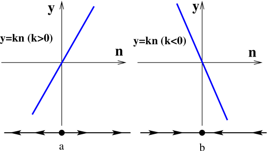
Figure 3.7:

Another example of an equation with parameters is the logistic equation for population growth (3.21). This equation depends on two parameters $r$ and $k$, where $r$ accounts for the growth rate and $k$ accounts for the carrying capacity. Let us consider a slight modification of equation (3.21) for a population which is subject to harvesting at a constant rate $h$:

$$dn/dt=r*n*(1-n/k)-h$$ (3.25)

where $h$ is the harvesting rate (an extra parameter).

Let us fix the parameters $r=2$ and $k=3$ (the same values as in equation (3.22)), and study only the effect of varying the harvesting parameter $h$ on, the dynamics of the population.

$$dn/dt=2*n*(1-n/3)-h$$ (3.26)

When $h=0$ equation (3.26) coincides with equation (3.22) which was studied in fig.3.5. Now assume that the harvesting $h$ is not zero. Let us plot graphs of $2*n*(1-n/3)-h$ for $h=0;h=0.8;h=1.6$ (fig.3.8a).

Figure 3.8:

The phase portraits for $h=0.0;h=0.8;h=1.6$ are shown in fig3.8b. We see that at $h=0.8$ the behavior of the system is qualitatively similar to the behavior of the system without harvesting ($h=0.0$): the population eventually approaches the stable non-zero equilibrium. However the final size of the population in this case is slightly smaller than for the population without harvesting (fig.3.5a) At $h=1.6$ the situation is different. We do not have a stable and non-stable equilibrium anymore. The flow is always directed to the left and the size of the population decreases. In this simple model this means the extinction of the population. The important question here is, what is the maximal possible harvesting rate at which the population still survives. From the previous analysis it is clear that the critical harvesting is reached when the parabola $2*n*(1-n/3)-h$ touches the $n$-axis (fig.3.8c). To find this critical value we note, that $h$ just shifts the parabola $2n(1-n/3)$ downward. Therefore, the situation of (fig.3.8c) occurs, when the shift equals the maximum of the parabola $2*n*(1-n/3)$. To find the maximal value we find a point where the derivative $df/dn=0$

$$\begin{array}[]{l}df/dn=2/3(3-n)-(2/3)*n*3=2-4n/3=0\\ n_{max}=3/2;\quad f(n_{max})=(2/3)*(3/2)*(3-3/2)=3/2\end{array}$$ (3.27)

So the maximal value of $(2/3)*n*(3-n)$ equals $3/2$ and therefore the maximal harvesting is $h=3/2$

If $h>3/2$ there are no equilibria and the population will go extinct. If $h<3/2$ there is a stable and non-stable equilibrium and the population will go to the stable equilibrium. At $h=3/2$ we are at a boundary between these two qualitatively different cases. Such a qualitative change in system behavior is called a bifurcation. Bifurcations are studied in a special section of mathematics: theory of dynamical systems.

3.4 Exercises

Exercises for section 3.1

1. Assume that a population grows in accordance with the following equation:

   $${dn\over dt}=1.5n$$

   If the initial size of the population was $n(0)=30$, find what will be size at time $t=4$. Find at what time the population will double its initial size.

2. A bacterial population doubles its size each 20 minutes. The growth of this population $N$ satisfies the differential equation ${dN\over dt}=kN$. Find the value of $k$ in $sec^{-1}$.

   Exercises for section 3.2

3. Study the listed differential equations by answering the following questions:

   • Draw the phase portrait.

   • How many equilibria do we have here? At which $x$?

   • For each equilibrium tell whether is it stable or non-stable

   • What will be the final value of $x$ if $t\rightarrow\infty$. (e.g. $x$ converges to equilibrium, or $x$ goes to infinity, etc.)

   • List attractor/attractors and determine their basin/basins of attraction.

   1. ${dx\over dt}=-15+8x-x^{2}$

   2. ${dx\over dt}=-4+5x-x^{2}$

   3. ${dx\over dt}=-x(x^{2}+x-6)$

   4. ${dx\over dt}=8x-x^{3}$

   5. ${dx\over dt}=f(x)$ with the following graphs of $f(x)$:

      

   6. ${dx\over dt}={3x^{2}\over 2+x^{2}}-x$ (this equation (Adler 1996) describes the dynamics of population of species which cannot bread successfully when numbers are too small or too large)

4. The following equation describes the production of a gene product with concentration $x$:

   $$dx/dt=-x(x-0.2)(x-1)+s$$

   Here $s$ is the parameter accounting for a chemical which produces the gene product. The initial state of the system was: $x=0$ and the value of $s=0$. At some moment of time the value of $s$ was slowly increased from $s=0$ to $s=s_{max}$ and then slowly decreased back to the value $s=0$.

   1. The value of function $-x(x-0.2)(x-1)$ at its local minimum is $-0.009$. (Optional) Show this from function derivative, or using calculator.

   2. What will be the value of the concentration of the gene product $x$ at the end of the described process for $s_{max}=0.005$?

   3. The same for $s_{max}=0.02$?

   4. Show that there is a critical value of $s_{max}$ that separates different outcomes of this process. Find this critical value of $s_{max}$.

5. Consider a model population with logistic growth which is subject to harvesting at a constant rate $h$

   $$dn/dt=r*n*(1-n/k)-h$$ (3.28)

   Find the maximal yield $h$.

   Additional Exercises

6. Assume that the growth of a mass of an animal can given by the following differential equation:

   $${dW\over dt}=400-0.3W$$

   where W is the weight in grams and $t$ time in weeks.

   1. Find the solution for the initial $W(0)=10$.

   2. At what time the mass will reach half of the saturated value.

   3. If we assume that the linear size of the animal is proportional to the cubic root of the mass, find at what time the object will reach half of its saturated linear size.

7. The dynamics of the ionic channels in the famous Hodgkin-Huxley model for a nerve cell is described by the following type of equations:

   $${dm\over dt}=\alpha(1-m)-\beta m$$

   where $m$ is a gating variable and $\alpha,\beta$ are the parameters.

   Find the steady state values of the gating variable $m$ and the characteristic time of approaching this steady state.

8. Consider a model where the harvesting $(hn)$ is proportional to the size of the population:

   $$dn/dt=r*n*(1-n/k)-hn$$ (3.29)

   Find the maximal yield.

9. Compare the harvesting strategies (3.28) and (3.29). Which strategy is better. Why?

Chapter 4 System of two linear differential equations

Many biological systems are described by several differential equations. One of the most simple types of such systems is a system of two linear differential equations that on a general form can be written as:

$$\left\{\begin{array}[]{l}{dx\over dt}=ax+by\\ {dy\over dt}=cx+dy\end{array}\right.$$ (4.1)

here $x(t)$ and $y(t)$ are unknown functions of time $t$, and $a,b,c,d$ are constants (parameters).

System (4.1) by itself has many practically important applications, for example compartmental models in biology and pharmacology, electrical circuits in physics, models in economics, etc. System (4.1) will also be very important for study so-called nonlinear system of differential equations which is widely used in theoretical biology and will be considered in chapter 5.

This chapter we will introduce main definitions for linear systems (phase portrait and equilibria points) we will derive a formula for general solution of this system and classify possible solutions of this system and their phase portraits. These results will be used later to study models of biological processes.

4.1 Phase portraits and equilibria

Let us consider an example of system (4.1) with particular values for the parameters $a,b,c,d$:

$$\left\{\begin{array}[]{l}{dx\over dt}=-2x+y\\ {dy\over dt}=x-2y\end{array}\right.$$ (4.2)

Let us first solve this system on a computer. For that we need to choose initial values for $x$ and $y$ and let the computer find their dynamics in the course of time. Solutions for $x(0)=1,y(0)=2$ are shown in fig.4.1. We see, that in the course of time, $x$ and $y$ approach the stationary values $x=0.,y=0.$

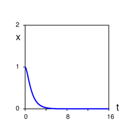
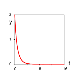
Figure 4.1:

Let us represent this solution graphically. For a differential equation with one variable $({dx\over dt}=f(x)$) we presented the solutions in terms of a one-dimensional phase portrait using the $x$-axis. For system with two variables, we need to use two axes to represent the dynamics. Let us consider a two dimensional coordinate system $Oxy$ with the $x$-axis for the variable $x$ and the $y$-axis for the variable y. Such a coordinate system is called a phase space. Let us represent the trajectory from fig.4.1 on the $Oxy$-plane. The initial sizes of the populations were $x(0)=1,y(0)=2$, thus we put this point ($1,2$) on the $Oxy$-plane. At the next moment of time we get other values for $x$ and $y$ and we also put them on the $Oxy$-plane and the $x$ and the $y$ coordinates of the next point, etc. Finally, we will get the line shown in fig.4.2a that starts at ($2,1$) and ends at ($0,0$). To show how $x$ and $y$ change in the course of time we draw an arrow as in fig.4.2a. This trajectory is the first element of the phase portrait. If we start trajectories from many different initial conditions we will get the complete phase portrait of system (4.2) (fig.4.2b). Each trajectory represents a certain type of dynamics of $x(t),y(t)$, which can be easily shown on time plots similar to fig.4.1. The phase portrait in fig.4.2b give us the overall qualitative dynamics of our system: the variables $x$ and $y$ approach $0,0$ from all possible initial conditions.

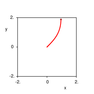
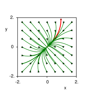
Figure 4.2:

Phase portrait of system (4.2): (${dx\over dt}=-2x+y;{dy\over dt}=x-2y$) found numerically.

The main aim of our course is to develop a procedure of drawing a phase portrait of a general system of two differential equations without using a computer which will allow us to study models of biological processes. In the 1D case the phase portrait consisted of two main elements: equilibria points and flows (trajectories) between them. Similar elements also compose the phase portrait of a system of two differential equations. Let us start with the first main element and define equilibria of the system.

In the 1D case equilibria were points where our system is stationary: placed at an equilibrium point the system will stay there forever. Mathematically equilibria for eq. ${dx\over dt}=f(x)$ (3.8) were determined as the points where ${dx\over dt}=0$, i.e. where $f(x)=0$. In the 2D case it is required that at the equilibrium point both variables $x$ and $y$ do not change their values, i.e. both ${dx\over dt}=0$ and ${dy\over dt}=0$. For system (4.2) these conditions give the following the system of two algebraic equations for finding equilibria:

t

$$\left\{\begin{array}[]{l}{dx\over dt}=0=-2x+y\\ {dy\over dt}=0=x-2y\end{array}\right.\begin{array}[]{l}\Rightarrow\end{array}\left\{\begin{array}[]{l}y=2x\\ x-2y=0\end{array}\right.\begin{array}[]{l}\Rightarrow\end{array}\left\{\begin{array}[]{l}y=2x\\ x-2*2x=0\end{array}\right.\begin{array}[]{l}\Rightarrow\end{array}\left\{\begin{array}[]{l}y=2x\\ -3x=0\end{array}\right.$$ (4.3)

that have the only solution $x=0,y=0$. Therefore system (4.2) has an equilibrium point $(0,0)$. As we see in fig.4.2b this equilibrium is an attractor for all trajectories.

For a general linear system (4.1) the equilibria will be given by:

$$\left\{\begin{array}[]{l}ax+by=0\\ cx+dy=0\end{array}\right.$$ (4.4)

This system always has a solution $x=0,y=0$ and thus the general linear system (4.1) always has an equilibrium at the point $x=0,y=0$. In the next sections we will find out how to sketch a phase portrait of (4.1) around this equilibrium. Our plan will be the following. We will first find the general analytical solution of this system and then will use it to draw the phase portraits.

4.2 General solution of linear system

Consider a general system of two differential equations with constant coefficients:

$$\left\{\begin{array}[]{l}{dx\over dt}=ax+by\\ {dy\over dt}=cx+dy\end{array}\right.$$ (4.5)

The general solution of (4.5) can be written in the following form

$$\left(\begin{array}[]{c}x\\ y\end{array}\right)=C_{1}\left(\begin{array}[]{c}v_{1x}\\ v_{1y}\end{array}\right)e^{\lambda_{1}t}+C_{2}\left(\begin{array}[]{c}v_{2x}\\ v_{2y}\end{array}\right)e^{\lambda_{2}t}$$ (4.6)

where $\lambda_{1},\lambda_{2}$ are eigen values of the matrix $A=\left(\begin{array}[]{lr}a&b\\ c&d\end{array}\right)$, and $\left(\begin{array}[]{c}v_{1x}\\ v_{1y}\end{array}\right)$, $\left(\begin{array}[]{c}v_{2x}\\ v_{2y}\end{array}\right)$ are the corresponding eigen vectors.

We will not derive the formula (4.6), we will show the main ideas behind the real derivation. For that let us consider first the one dimensional case, and then extend it to a two dimensional system.

The easiest way to find solutions of system (4.5) is by the method of substitution. Let us illustrate this method on example of 1D analog of system (4.5) which is 1D linear differential equation:

$${dx\over dt}=ax$$ (4.7)

We can easily solve (4.7) using the direct method of separation of variables and subsequent integration. However, let us find the solution using another method, the method of substitution. The main idea of this method is to look for a solution in some known class of functions which should be chosen in advance from some preliminary analysis. It was found that for linear systems this class is the class of exponential functions $Ce^{\lambda t}$. Important questions such as: how was this class found and is this class unique etc, will not be discussed. Our aim here will be an illustration of the main components of the solution rather than comprehensive analysis of linear systems, which is a large special section of mathematics. Once the class of functions is given (in our case the class of exponential functions), we need to check under which circumstances it will satisfy the equations we are solving. Thus we will look for a solution of (4.7) of the form $x=Ce^{\lambda t}$, where $C$ and $\lambda$ are unknown coefficients. The main idea of the method of substitution is to find these unknown coefficients for a particular system. Let us substitute $x=Ce^{\lambda t}$ into (4.7). We find: ${dx\over dt}=(Ce^{\lambda t})^{\prime}=\lambda Ce^{\lambda t}$ , or:

$$\lambda Ce^{\lambda t}=aCe^{\lambda t}$$

We can cancel $e^{\lambda t}$ and $C$, and we get:

$$\lambda=a$$ (4.8)

Hence we found the following the solutions of (4.7):

$$x=Ce^{at}$$ (4.9)

where $C$ is an arbitrary constant.

Now, let us use the same approach for the two dimensional system (4.5). It turns out that the class of functions in two dimensions will be the same as in one dimension, but because we have two variables, we need to introduce different constants for $x$ and $y$, so our substitution will be

$$x=C_{x}e^{\lambda t};y=C_{y}e^{\lambda t}\quad or\quad\left(\begin{array}[]{c}x\\ y\end{array}\right)=\left(\begin{array}[]{c}C_{x}\\ C_{y}\end{array}\right)e^{\lambda t}$$ (4.10)

where $C_{x},C_{y},\lambda$ are unknown coefficients. Let us make this substitution for a particular example:

$$\left(\begin{array}[]{c}{dx\over dt}\\ {dy\over dt}\end{array}\right)=\left(\begin{array}[]{lr}1&4\\ 1&1\end{array}\right)\left(\begin{array}[]{c}x\\ y\end{array}\right)$$ (4.11)

Substitution for ${dx\over dt}=\lambda C_{x}e^{\lambda t},{dy\over dt}=\lambda C_{y}e^{\lambda t},x=C_{x}e^{\lambda t},y=C_{y}e^{\lambda t}$ gives:

$$\left\{\begin{array}[]{l}\lambda C_{x}e^{\lambda t}=C_{x}e^{\lambda t}+4C_{y}e^{\lambda t}\\ \lambda C_{y}e^{\lambda t}=C_{x}e^{\lambda t}+C_{y}e^{\lambda t}\end{array}\right.$$ (4.12)

we can cancel $e^{\lambda t}$, (but not $C_{x},C_{y}$ as in one dimensional case), and get:

$$\left\{\begin{array}[]{l}\lambda C_{x}=C_{x}+4C_{y}\\ \lambda C_{y}=C_{x}+C_{y}\end{array}\right.$$ (4.13)

or in the matrix form:

$$\lambda\left(\begin{array}[]{c}C_{x}\\ C_{y}\end{array}\right)=\left(\begin{array}[]{lr}1&4\\ 1&1\end{array}\right)\left(\begin{array}[]{c}C_{x}\\ C_{y}\end{array}\right)$$ (4.14)

We see that to find the solution of (4.11) we need to solve the problem (4.14), which is the eigen value problem considered in section 2.3. To solve it we find eigen values from the characteristic equation (2.31): $Det\left|\begin{array}[]{lr}1-\lambda&4\\ 1&1-\lambda\end{array}\right|=(1-\lambda)*(1-\lambda)-4=\lambda^{2}-2\lambda-3=0\;\;\lambda_{12}={2\pm\sqrt{2^{2}+3*4}\over 2}=1\pm{1\over 2}\sqrt{16}=1\pm 2$. Hence $\lambda_{1}=-1,\lambda_{2}=3$

We use the express formula (2.36) for eigen vectors and get:

$$\lambda_{1}=-1;\left(\begin{array}[]{c}v_{1x}\\ v_{1y}\end{array}\right)=\left(\begin{array}[]{c}-4\\ 1-(-1)\end{array}\right)=\left(\begin{array}[]{c}-4\\ 2\end{array}\right)\quad\lambda_{2}=3;\left(\begin{array}[]{c}v_{2x}\\ v_{2y}\end{array}\right)=\left(\begin{array}[]{c}-4\\ -2\end{array}\right).$$ (4.15)

Formula (4.15) gives just one eigen vector for each eigen value. We also know (see formula (2.33 in section 2.3) that all eigen vectors can be found by multiplication of this eigen vector by an arbitrary constant. If we denote by $C_{1}$ the constant for the first eigen vector and by $C_{2}$ the constant for the second eigen vector we will get the following solution of the eigen value problem (4.14):

$$\lambda_{1}=-1;\left(\begin{array}[]{c}v_{1x}\\ v_{1y}\end{array}\right)=C_{1}\left(\begin{array}[]{c}-4\\ 2\end{array}\right)\quad\lambda_{2}=3;\left(\begin{array}[]{c}v_{2x}\\ v_{2y}\end{array}\right)=C_{2}\left(\begin{array}[]{c}-4\\ -2\end{array}\right).$$ (4.16)

If we substitute these eigen vectors into the formula (4.10) we find the following solutions of (4.11)

$$\left(\begin{array}[]{c}x\\ y\end{array}\right)=C_{1}\left(\begin{array}[]{c}-4\\ 2\end{array}\right)e^{-1*t}\quad\left(\begin{array}[]{c}x\\ y\end{array}\right)=C_{2}\left(\begin{array}[]{c}-4\\ -2\end{array}\right)e^{3*t}$$ (4.17)

Now let us prove the following property of system (4.5):
$\bullet$ If $x_{1},y_{1}$ and $x_{2},y_{2}$ are two solutions of (4.5), then $x_{1}+x_{2},y_{1}+y_{2}$ is also a solution of (4.5).
Proof: As $x_{1},y_{1}$ and $x_{2},y_{2}$ are the solution this means that they satisfy (4.5), i.e.

$$\left\{\begin{array}[]{l}{dx_{1}\over dt}=ax_{1}+by_{1}\\ {dy_{1}\over dt}=cx_{1}+dy_{1}\end{array}\right.\qquad\left\{\begin{array}[]{l}{dx_{2}\over dt}=ax_{2}+by_{2}\\ {dy_{2}\over dt}=cx_{2}+dy_{2}\end{array}\right.$$ (4.18)

If we add equations for ${dx_{1}\over dt}$ and ${dx_{2}\over dt}$ we get: ${dx_{1}\over dt}+{dx_{2}\over dt}=ax_{1}+by_{1}+ax_{2}+by_{2}$, which can be re-written as: ${d(x_{1}+x_{2})\over dt}=a(x_{1}+x_{2})+b(y_{1}+y_{2})$. If we do the same for equations for ${dy_{1}\over dt}$ and ${dy_{2}\over dt}$ we will finally get:

$$\left\{\begin{array}[]{l}{d(x_{1}+x_{2})\over dt}=a(x_{1}+x_{2})+b(y_{1}+y_{2})\\ {d(y_{1}+y_{2})\over dt}=c(x_{1}+x_{2})+d(y_{1}+y_{2})\end{array}\right.$$ (4.19)

which explicitly shows that $x_{1}+x_{2},y_{1}+y_{2}$ is a solution of (4.5).

If we apply this result for two found solutions (4.17) of (4.11) we can conclude that the sum of these two solutions is also a solution of (4.11):

$$\left(\begin{array}[]{c}x\\ y\end{array}\right)=C_{1}\left(\begin{array}[]{c}-4\\ 2\end{array}\right)e^{-1*t}+C_{2}\left(\begin{array}[]{c}-4\\ -2\end{array}\right)e^{3*t}$$ (4.20)

We proved formula (4.6) for a particular system. If we apply the same steps for a general system (4.5) we will get the general solution in the form (4.6).

So, we solved system (4.5). In the next sections we will find out how to draw its phase portraits.

4.3 Real eigen values. Saddle, node.

As we know, the general solution of (4.1) is given by (4.6). We can use this formula to sketch a phase portrait of this system. It turns out, that we can have several different types of equilibria depending on the eigen values $\lambda_{1},\lambda_{2}$. As we know $\lambda_{1},\lambda_{2}$ are the roots of the characteristic equation (2.31), which is a general quadratic equation. Therefore, the roots can be real or complex numbers. In this section we consider the case of real roots.

So, assume that the eigen values $\lambda_{1}$ and $\lambda_{2}$ are real. This yields the following three cases:

1. Eigen values have different signs ($\lambda_{1}<0;\lambda_{2}>0$, or $\lambda_{1}>0;\lambda_{2}<0$).

2. Both eigen values are positive ($\lambda_{1}>0;\lambda_{2}>0$)

3. Both eigen values are negative ($\lambda_{1}<0;\lambda_{2}<0$)

Note, that we do not consider the case when $\lambda=0$. This situation is quite rare and is not considered in this course.

4.3.1 Saddle; $\lambda_{1}<0;\lambda_{2}>0$, or $\lambda_{1}>0;\lambda_{2}<0$

System (4.11), which we solved in section 4.2, had eigen values $\lambda_{1}=-1,\lambda_{2}=3$. Let us draw its phase portrait. The general solution of this system is given by (4.20)

$$\left(\begin{array}[]{c}x\\ y\end{array}\right)=C_{1}\left(\begin{array}[]{c}-4\\ 2\end{array}\right)e^{-1*t}+C_{2}\left(\begin{array}[]{c}-4\\ -2\end{array}\right)e^{3*t}.$$ (4.21)

Because $C_{1},C_{2}$ are arbitrary constants let us consider three simple cases, in which one of these constants, or both of them are zero.

1) If $C_{1}=0,C_{2}=0$, then $x=0,y=0$ and do not depend on time. The trajectory is just one point (0,0), which is the equilibrium point of the system (4.11).

2) If $C_{1}=0,C_{2}=$ any number, then $\left(\begin{array}[]{c}x\\ y\end{array}\right)=C_{2}\left(\begin{array}[]{c}2\\ 1\end{array}\right)e^{3*t}$. Because $e^{3*t}$ can change from 1 (at $t=0$) to any infinitely large number and $C_{2}$ is an arbitrary positive or negative number, this expression can be rewritten as:

$$\left(\begin{array}[]{c}x\\ y\end{array}\right)=C_{2}\left(\begin{array}[]{c}-4\\ -2\end{array}\right)e^{3*t}=\left(\begin{array}[]{c}-4\\ -2\end{array}\right)K={\bf V_{2}}K$$ (4.22)

where $K$ is an arbitrary number from $-\infty<K<\infty$ and ${\bf V_{2}}$ is a vector $\left(\begin{array}[]{c}-4\\ -2\end{array}\right)$. Thus expression (4.22) means multiplying of the eigen vector ${\bf V_{2}}$ by an arbitrary number $K$. In general, if we multiply a vector by a positive number $K$ we get a vector with the same direction but the length will be increased $K$ times. If we multiply the vector by a negative number, the direction of the vector will be changed to the opposite and the length will be changed by a factor $|K|$. Because in (4.22) $K$ assumes all values from $-\infty<K<\infty$, this will give a straight line along this vector $\left(\begin{array}[]{c}2\\ 1\end{array}\right)$ (fig.4.3a). To complete drawing the trajectory we need to show arrows indicating the motion of a point along the trajectory in the course of time. Because time dynamics is given by $e^{3t}$, $|K|$ in (4.22) will grow in the course of time, i.e. it will become either more positive, or more negative depending on its initial sign. Geometrically this means that a point will move apart from the origin of the $Oxy$ coordinate system and we will get a picture as in fig.4.3b.

Figure 4.3:

3) The third case is $C_{1}=\;$any number, $C_{2}=0$. The solution in this case is

$$\left(\begin{array}[]{c}x\\ y\end{array}\right)=C_{1}\left(\begin{array}[]{c}-4\\ 2\end{array}\right)e^{-t}.$$ (4.23)

As in previous case we conclude, that all trajectories in this case will be located on a straight line along the vector $\left(\begin{array}[]{c}-4\\ 2\end{array}\right)$ and we just need to show the direction of flow along this line. In this case, time dynamics is given by the function $e^{-t}$, which approaches zero when $t$ goes to infinity. Therefore, independent of initial conditions (independent of the value of $C_{1}$) we will approach the point $x=0,y=0$, and the arrows will have the following direction (fig.4.4).

Figure 4.4:

Finally let us draw the phase portrait for arbitrary $C_{1}$ and $C_{2}$ (fig.4.4b). Let us consider one trajectory for which $C_{1}\neq 0;C_{2}\neq 0$, for example: $C_{1}=0.1,\;C_{2}=0.1$. The solution in this case is given by:

$$\left(\begin{array}[]{c}x\\ y\end{array}\right)=0.1\left(\begin{array}[]{c}-4\\ 2\end{array}\right)e^{-t}+0.1\left(\begin{array}[]{c}-4\\ -2\end{array}\right)e^{3t}$$ (4.24)

This trajectory starts as point $x=-0.4+0.2=-0.2;\;y=0.2-0.1=0.1$. In the course of time $e^{-t}$ will become smaller and smaller, while $e^{3t}$ will grow. So, the first term in (4.24) $0.1\left(\begin{array}[]{c}-4\\ 2\end{array}\right)e^{-t}$ will be small compared to the second term $0.1\left(\begin{array}[]{c}-4\\ -2\end{array}\right)e^{3t}$, and the dynamics at large $t$ will be described by an approximate formula : $\left(\begin{array}[]{c}x\\ y\end{array}\right)\approx 0.1\left(\begin{array}[]{c}-4\\ -2\end{array}\right)e^{3t}$, thus the trajectory will approach the line (4.22) presented in fig.4.3b. There will be similar behavior for any other trajectories: independently on staring points they will approach line of fig.4.3b from various directions. The qualitative picture will be as in fig.4.4b.

Such a phase portrait is called a saddle point. It has the following important features: (1) There is an equilibrium point at $x=0,y=0$. (2) There are two lines associated with eigen vectors of our system (fig.4.3b,fig.4.4a). These lines are called manifolds. The manifolds in fig.4.3b and fig.4.4a are different. If we follow the trajectory along the manifold in fig.4.3b the distance to the equilibrium increases (see fig.4.4). On the contrary, if we follow the trajectory along the manifold in fig.4.4a the distance to the equilibrium decreases. The manifold from fig.4.3b is called a non-stable manifold. The manifold from fig.4.4a is called a stable manifold.

Conclusions of this study can be easily generalized. If we consider an expression:

$$\left(\begin{array}[]{c}x\\ y\end{array}\right)=C\left(\begin{array}[]{c}v_{x}\\ v_{y}\end{array}\right)e^{\lambda t},$$ (4.25)

it will obviously determine a manifold (straight line) along the vector $\left(\begin{array}[]{c}v_{x}\\ v_{y}\end{array}\right)$ and the stability of this manifold will be determined by $e^{\lambda t}$. There are two main types of behavior of the function $e^{\lambda t}$ (fig.4.5). If $\lambda<0,e^{\lambda t}$ approaches zero, when $t$ increases. If $\lambda>0,e^{\lambda t}$ grows to infinity with increasing $t$. Hence, if $\lambda<0$, eq.(4.25) will determine a stable manifold: $x,y$ will approach $0$ in the course of time (as in fig.4.4a). If $\lambda>0$, then $x,y$ will diverge to infinity and we will get a non-stable manifold.

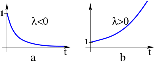
Figure 4.5:

Conclusion 1

The equation (4.25) on a phase portrait gives a manifold in the form of a straight line. This line goes through the origin and is directed along the vector $\left(\begin{array}[]{c}v_{x}\\ v_{y}\end{array}\right)$. This manifold is stable if $\lambda<0$ and non-stable if $\lambda>0$.

Finally the formal definition of a saddle point:

Conclusion 2

Fig.4.4 shows the phase portrait of a saddle point. It occurs close to equilibrium, at which eigen values of the system are real and have different signs, i.e. $\lambda_{1}<0;\lambda_{2}>0$, or $\lambda_{1}>0;\lambda_{2}<0$. The phase portrait of a saddle point has two manifolds directed along the eigen vectors. One manifold is stable (corresponding to the negative eigen value of the system). The other manifold is non-stable (corresponding to the positive eigen value of the system).

4.3.2 Non-stable node; $\lambda_{1}>0;\lambda_{2}>0$

Let us draw the phase portrait for the case when eigen values are real and are both positive. The general solution of the system is given by (4.6):

$$\left(\begin{array}[]{c}x\\ y\end{array}\right)=C_{1}\left(\begin{array}[]{c}v_{1x}\\ v_{1y}\end{array}\right)e^{\lambda_{1}t}+C_{2}\left(\begin{array}[]{c}v_{2x}\\ v_{2y}\end{array}\right)e^{\lambda_{2}t}$$ (4.26)

From the previous analysis we immediately conclude, that the phase portrait in this case has the equilibrium point at $(0,0)$ and two unstable manifolds along the vectors $\left(\begin{array}[]{c}v_{1x}\\ v_{1y}\end{array}\right)$ and $\left(\begin{array}[]{c}v_{2x}\\ v_{2y}\end{array}\right)$ (fig.4.6a). Let us put that on the graph (fig.4.6b).

Figure 4.6:

To complete the picture we need to add several trajectories which start between the manifolds. For such trajectories $C_{1}\neq 0\;C_{2}\neq 0$ and both terms in (4.26) will diverge to plus or minus infinity. So, we get trajectories as in fig.4.6b. Such an equilibrium is called a non-stable node.

Conclusion 3

If the eigen values of system (4.1) are real and both positive ($\lambda_{1}>0,\lambda_{2}>0$) we have an equilibrium point called a non-stable node. To draw a phase portrait at this equilibrium we need to show two non-stable manifolds along the eigen vectors of system (4.1) and add several diverging trajectories between the manifolds.

4.3.3 Stable node; $\lambda_{1}<0;\lambda_{2}<0$

The general solution in this case has the same form (4.26). The phase portrait will be similar to fig.4.6, but because $\lambda_{1}<0;\lambda_{2}<0$ both manifolds will be stable. So we get a picture fig.4.7a

Figure 4.7:

If the trajectory starts between the manifolds $(C_{1}\neq 0\;C_{2}\neq 0)$ it will also approach equilibrium as both terms in (4.26) will converge to 0, because $\lambda_{1}<0;\lambda_{2}<0$ (fig.4.7b). Such an equilibrium is called a stable node.

Conclusion 4

If the eigen values of system (4.1) are real and both negative ($\lambda_{1}<0,\lambda_{2}<0$) we have an equilibrium point called stable node. To draw a phase portrait at this equilibrium we need to show two stable manifolds along the eigen vectors of system (4.1) and add several trajectories converging to the equilibrium (0,0).

4.4 Phase portraits for complex eigen values: spiral, center

In the previous section we have studied the case when the roots of the characteristic equation (2.31) are real, and found three possible types of phase portrait (equilibria): saddle, stable node and unstable node. Here we will study the case when the roots of the characteristic equation (2.31) are complex.

4.4.1 General ideas on equilibria with complex eigenvalues

From section 4.2 we know that in order to find the type of phase portrait of linear system we need to solve the characteristic equation (2.31) which is a general quadratic equation, and because the parameters $a,b,c,d$ of the linear system are arbitrary the coefficients of the characteristic equation are also arbitrary. Therefore, it may happen that the discriminant of this quadratic equation will be negative and we will have complex eigen values. From equation (2.7) we know that these eigen values will be given by

$$\lambda_{1}={-B+i\sqrt{-D}\over 2}\quad\lambda_{2}={-B-i\sqrt{-D}\over 2}$$ (4.27)

or if we denote the real part of these complex numbers as : $\alpha={-B\over 2}$ and the imaginary part as $\beta={\sqrt{-D}\over 2}$ we can rewrite (4.27) as

$$\lambda_{1,2}=\alpha\pm i\beta$$ (4.28)

Which type of dynamics do we expect here. If we drop for a while the imaginary part $i\beta$ in (4.28), we get that $\lambda_{1}=\lambda_{2}=\alpha$, i.e. both eigen values will be the same and hence they will have the same sign. Which type of equilibria do we have for two real eigen values which have the same sign? We can have either a non-stable node if $\lambda_{1}>0,\lambda_{2}>0$ , or a stable node, if $\lambda_{1}<0,\lambda_{2}<0$ (see section 4.2). In the case of a non-stable node all the trajectories diverge from the equilibrium (fig.4.6b), while in the case of a stable node all the trajectories converge to it (fig.4.7b). It turns out that we will get similar behavior for complex eigen values: if $Re\lambda_{1,2}>0$ we will get divergence of the trajectories, if $Re\lambda_{1,2}<0$ we will get convergence of the trajectories to the equilibrium. However, the picture will be slightly different from fig.4.6b and fig.4.7b, as the imaginary part of the eigen values $Im\lambda_{1,2}$ will add rotation to the trajectories.

The complete derivation of the formula for the general real solution of system (4.1) with complex eigen values is given in the appendix at the end of this chapter for extra reading. Here we will just demonstrate that $Im\lambda_{1,2}$ adds rotation.

4.4.2 Center, spiral

Let illustrate that the imaginary part of the complex eigen value of the characteristic equation results in a rotation of the trajectories. For that let us consider a system:

$$\left(\begin{array}[]{c}{dx\over dt}\\ {dy\over dt}\end{array}\right)=\left(\begin{array}[]{lr}0&2\\ -2&0\end{array}\right)\left(\begin{array}[]{c}x\\ y\end{array}\right)\qquad or\qquad\left\{\begin{array}[]{l}{dx\over dt}=2y\\ {dy\over dt}=-2x\end{array}\right.$$ (4.29)

In this case the eigen values are given by: $Det\left|\begin{array}[]{lr}-\lambda&2\\ -2&-\lambda\end{array}\right|=\lambda^{2}+4=0\;\;\lambda_{1,2}=\pm 2i$. Thus we have purely imaginary eigen values. It turns out that we can draw a phase portrait of this system using the following trick. Let us multiply the first equation in (4.29) by $x$, the second equation by $y$ and let us add them together. We get

$$\begin{array}[]{l}x{dx\over dt}=x2y\\ +\\ y{dy\over dt}=-y2x\\ gives\\ x{dx\over dt}+y{dy\over dt}=2xy-2xy=0\end{array}$$ (4.30)

Now note that

$$x{dx\over dt}={1\over 2}{dx^{2}\over dt}$$

(just check this by applying the chain rule for ${dx^{2}\over dt}$), and similarly

$$y{dy\over dt}={1\over 2}{dy^{2}\over dt}$$

hence eq.(4.30) can be rewritten as:

$$\begin{array}[]{l}{1\over 2}{dx^{2}\over dt}+{1\over 2}{dy^{2}\over dt}=0\\ \\ {d(x^{2}+y^{2})\over dt}=0\end{array}$$

We know that if the derivative of the function $f$ is zero (${df\over dt}=f^{\prime}(x)=0$) then the function $f$ is a constant, thus the above equation implies:

$$x^{2}+y^{2}=Const$$ (4.31)

Expression (4.31) gives a so-called first integral of our system: combination of variables which are preserved in time. It is not equivalent to the solution of our system, but using it we can draw the phase portrait of system (4.29).

Because $Const$ in (4.31) is an arbitrary positive number, let us denote it as $Const=A^{2}$, where $A$ is just another arbitrary constant. Thus we will get the equation $x^{2}+y^{2}=A^{2}$, which represents a graph of a circle with radius $A$ and with the center at the origin (fig.4.8a).

Figure 4.8:

To find the dynamics on this circle let us find ${dy\over dt}$ at a point $x=A,y=0$ (the bold point in fig.4.8a). From eq.(4.29 ${dy\over dt}=-2x=-2A<0$, i.e. the coordinate $y$ decreases at this point in the course of time. Thus we conclude that motions of trajectory along the circle will be in the clockwise direction. If we draw a series of such circles for different $A$ we will get the phase portrait as shown in fig.4.8b. The dynamics of the $x$ and $y$ variables can be found by considering motion along trajectories of the system: motion here is a rotation of a point along the circle. During this rotation the variable $x$ changes periodically (between the values $+A$ and $-A$), and thus we will see periodic oscillations. The same is valid for the variable $y$. An example of such dynamics is represented in fig.4.8c. The equilibrium point $(0,0)$ in such system is called a center. The phase portrait in Fig.4.8 is a set of circles, which is a consequence of the symmetry of system (4.29). In a general case, if $\lambda_{1,2}=\pm i\beta$, we will also get a center point, similar to that in fig.4.8, but instead of circles we can get a series of embedded ellipses. The dynamics of the variables will always be oscillations.

Conclusion 5

If the eigen values of system (4.1) are $\lambda_{1,2}=\pm i\beta$, we have an equilibrium point called a center. The dynamics of variables $x,y$ are oscillations. The phase portrait is a set of embedded ellipses.

A computer generated phase portrait of the system ${dx\over dt}=-x-2y;{dy\over dt}=x+y$ is shown in fig.4.10a. The eigen values in this case are $\lambda_{1,2}=\pm i0.1$. The time-plot for the $x$ and $y$ variables is shown in fig.4.10(left).

Conclusion 6

The imaginary part of the eigen values results in the rotation of trajectories on a phase portrait.

Now let us consider the next two cases: $\lambda_{1,2}=\alpha\pm i\beta$.

As we discussed in section 4.3, $Re\lambda_{1,2}$ determines convergence or divergence of the trajectories to the equilibrium. In the case $\lambda_{1,2}=\alpha\pm i\beta;\alpha<0$ we expect that the real part of the eigenvalue will give a behavior similar to the case of both negative real eigenvalues, hence we expect the convergence of trajectories to the equilibrium, as for a stable node. In addition to this, as we saw in the previous section, the imaginary part of the eigen values causes the rotation of the trajectory. If we add these two processes together we will get convergence to the equilibrium with rotation, hence trajectories will have the form of spirals. A computer generated phase portrait for this case is shown in fig.4.10b. The system is ${dx\over dt}=-x-2y;{dy\over dt}=x+0.7y$. The eigen values in this case are $\lambda_{1,2}=-0.15\pm i0.13$. The time-plot for the $x$ and $y$ variables is shown in fig.4.10(middle). The dynamics of the system are oscillations with gradually decreasing amplitude.

Conclusion 7

If the eigen values of system (4.1) are $\lambda_{1,2}=\alpha\pm i\beta;\alpha<0$, we have an equilibrium point called a stable spiral, fig.4.10b.

The last case occurs if $\lambda_{1,2}=\alpha\pm i\beta;\alpha>0$. This case is similar to the previous one. The only difference is that because $Re\lambda_{1,2}=\alpha>0$, the real part gives motion equivalent to a non-stable node, or divergence of trajectories from the equilibrium. So, together with rotation from the imaginary part of $\lambda$ we get the following phase portrait (fig.4.10c). This phase portrait is generated by computer for the system ${dx\over dt}=-x-2y;{dy\over dt}=x+1.2y$. The eigen values in this case are $\lambda_{1,2}=0.1\pm i0.89$. The time-plot for the $x$ and $y$ variables is shown in fig.4.10(right). The dynamics of the system are oscillations with gradually increasing amplitude.

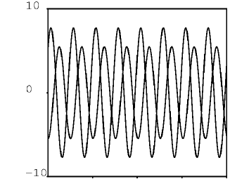
Figure 4.9:

Figure 4.10: The dynamics of variables $x$ and $y$ for the phase portraits shown in fig.4.10. The left picture corresponds to the equilibrium point center, the middle picture corresponds to the equilibrium point stable spiral and the right picture corresponds to the equilibrium point non-stable spiral.

Conclusion 8

If the eigen values of system (4.1) are $\lambda_{1,2}=\alpha\pm i\beta;\alpha>0$, we have an equilibrium point called a non-stable spiral, fig.4.10c.

We have found all possible types of equilibria which can occur in 2D systems: saddle, non-stable node, stable node, center, non-stable spiral and stable spiral. The next question which we will discuss here is the stability of these equilibria.

4.5 Stability of equilibrium

We will call an equilibrium point stable, if there is a neighborhood of this equilibrium, such that all trajectories which start in this neighborhood will converge to the equilibrium (Fig.4.11a). We will call the equilibrium point non-stable, if there is at least one diverging trajectory from the close neighborhood of this equilibrium (fig.4.11b).

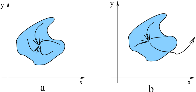
Figure 4.11:

If we analyze the stability of the 6 types of equilibria studied in the previous section we find the following:

Stable equilibria

1. Stable node $\lambda_{1}<0;\lambda_{2}<0$ real

2. Stable spiral $\lambda_{1,2}=\alpha\pm i\beta;\alpha<0$

Non-stable equilibria

1. Non-stable node $\lambda_{1}>0;\lambda_{2}>0$ real

2. Non-stable spiral $\lambda_{1,2}=\alpha\pm i\beta;\alpha>0$

3. Saddle point $\lambda_{1}<0;\lambda_{2}>0$; or $\lambda_{1}>0;\lambda_{2}<0$ real

In case of spirals and nodes the stability and non-stability is obvious. In case of a saddle point we have a converging trajectory, however the existence of the diverging trajectories (fig.4.4b) implies that this equilibrium point is non-stable. The last case, $\lambda_{1,2}=\pm i\beta$ (center point), is non conclusive. Trajectories do not converge and do not diverge from the equilibrium. Usually this case is treated as neutrally stable. All these cases can be formulated in the following theorem.

Theorem 1

If all eigenvalues of the linear system (4.1) have negative real parts, then the equilibrium point $x=0,y=0$ is stable.

It is easy to see, that this theorem includes all listed stable equilibria. It obviously works for a stable spiral, but it also works for a stable node, because any real number can be considered as a complex number with imaginary part equal to zero. For example: $-3$ can be represented as $z=-3=-3+i0$, and $Rez=-3;Imz=0$.

4.6 Exercises

Exercises for section 4.2

1. Find the general solution of the following systems of ordinary differential equations:

   1. $\left(\begin{array}[]{c}{dx\over dt}\\ {dy\over dt}\end{array}\right)=\left(\begin{array}[]{lr}-2&1\\ 1&-2\end{array}\right)\left(\begin{array}[]{c}x\\ y\end{array}\right)$

   2. $\left(\begin{array}[]{c}{dx\over dt}\\ {dy\over dt}\end{array}\right)=\left(\begin{array}[]{lr}3&-1\\ -2&4\end{array}\right)\left(\begin{array}[]{c}x\\ y\end{array}\right)$

2. Find the solution for the following initial value problem:

   $$\left(\begin{array}[]{c}{dx\over dt}\\ {dy\over dt}\end{array}\right)=\left(\begin{array}[]{lr}1&-2\\ 5&8\end{array}\right)\left(\begin{array}[]{c}x\\ y\end{array}\right)\quad\left(\begin{array}[]{c}x(0)\\ y(0)\end{array}\right)=\left(\begin{array}[]{c}3\\ -3\end{array}\right)$$

   (Hint: See an example of solution in section 11.0.1).

3. Two different concentrations of a solution are separated by a membrane through which the solute can diffuse. The rate at which the solute diffuses is proportional to the difference in concentrations between two solutions. The differential equations governing the process are:

   $$\left\{\begin{array}[]{l}dC_{1}/dt=-{k\over V_{1}}(C_{1}-C_{2})\\ dC_{2}/dt={k\over V_{2}}(C_{1}-C_{2})\end{array}\right.$$

   where $C_{1}$ and $C_{2}$ are the two concentrations, $V_{1}$ and $V_{2}$ are the volumes of the respective compartments, and $k$ is a constant of proportionality. If $V_{1}=20liters$, $V_{2}=5liters$, and $k=0.2\;liters/min$ and if initially $C_{1}=3\;moles/liter$ and $C_{2}=0$, find $C_{1}$ and $C_{2}$ as functions of time.

   Exercises for sections 4.3 and 4.4

4. Find eigen values and eigen vectors (for real eigen values only) of the following systems. Determine equilibrium type and sketch phase portraits. For real eigen values show non-stable, stable manifolds and several trajectories between the manifolds.

   1. $\left\{\begin{array}[]{l}{dx\over dt}=x+4y\\ {dy\over dt}=2x+3y\end{array}\right.$

   2. $\left\{\begin{array}[]{l}{dx\over dt}=5x-y\\ {dy\over dt}=3x+y\end{array}\right.$

   3. $\left\{\begin{array}[]{l}{dx\over dt}=3x-5y\\ {dy\over dt}=x-y\end{array}\right.$

   4. $\left\{\begin{array}[]{l}{dx\over dt}=-2x+y\\ {dy\over dt}=x-2y\end{array}\right.$

   5. $\left\{\begin{array}[]{l}{dx\over dt}=-2y\\ {dy\over dt}=x-2y\end{array}\right.$

   6. $\left\{\begin{array}[]{l}{dx\over dt}=-x-y\\ {dy\over dt}=2x+y\end{array}\right.$

   7. $\left\{\begin{array}[]{l}{dx\over dt}=-2x-y\\ {dy\over dt}=3x+2y\end{array}\right.$

5. Study the following linear system with a parameter $a$:

   $$\left\{\begin{array}[]{l}{dx\over dt}=-2x-ay\\ {dy\over dt}=3x-y\end{array}\right.$$

   Find the types of equilibrium which are possible for different values of $-\infty<a<\infty$. Give the parameter region for each equilibrium and draw qualitative phase portraits. For which parameter values is the equilibrium stable?

6. For which values of parameters $a$ and $b$ does the following system has periodic oscillations (i.e. a center equilibrium point):

   $$\left\{\begin{array}[]{l}{dx\over dt}=-ax+y\\ {dy\over dt}=(2a-3)x-by\end{array}\right.$$

7. Compartmental models play an important role in different parts of population biology, pharmacology and biochemistry. They describe the interaction between several processes, which may be interactions of populations, chemical reactions, etc. A two compartment model is schematically shown in fig.4.12. It represents two interacting species $x$ and $y$. The concentration of the species $x$ can be changed either due to a transition to species $y$ with the rate given by $ax$, or $x$ can die with the rate $cx$. Similar transitions exist also for the species $y$. The rates of these processes are specified in the figure.

   

   Figure 4.12:

   1. Derive a system of two differential equations for species $x$ and $y$.

   2. If $a=0.5,b=2,c=4.5,e=3$ find equilibrium type. Is it stable?

   3. Determine the stability of the equilibrium in a general case when $a>0,b>0,c>0,e>0$

4.7 Additional concepts (appendix)

4.7.1 General solution for complex eigen values

Notes about general solution of a system with complex eigenvalues

It turns out that if $\lambda_{1,2}=\alpha\pm i\beta$ formula (4.6) is still valid, so the solution can be represented in the form:

$$\left(\begin{array}[]{c}x\\ y\end{array}\right)=C_{1}\left(\begin{array}[]{c}v_{1x}\\ v_{1y}\end{array}\right)e^{\lambda_{1}t}+C_{2}\left(\begin{array}[]{c}v_{2x}\\ v_{2y}\end{array}\right)e^{\lambda_{2}t}$$ (4.32)

but as $\lambda_{1}=\alpha+i\beta;\lambda_{2}=\alpha-i\beta$ we get

$$\left(\begin{array}[]{c}x\\ y\end{array}\right)=C_{1}\left(\begin{array}[]{c}v_{1x}\\ v_{1y}\end{array}\right)e^{(\alpha+i\beta)t}+C_{2}\left(\begin{array}[]{c}v_{2x}\\ v_{2y}\end{array}\right)e^{(\alpha-i\beta)t}$$ (4.33)

This expression gives the correct solutions of (4.5). However, the form of the solution is not good. First, because $\lambda_{1,2}$ are complex, the eigenvectors $\left(\begin{array}[]{c}v_{1x}\\ v_{1y}\end{array}\right)$ and $\left(\begin{array}[]{c}v_{2x}\\ v_{2y}\end{array}\right)$ will also be complex. Next, we should consider $C_{1},C_{2}$ as general complex constants. Therefore (4.33) is a quite complicated expression which gives $x$ and $y$ as complex valued functions of time $t$. Mathematically it is correct and if we substitute (4.33) into the original equation (4.5) we get an equality. However, we need to draw a phase portrait of (4.5) on the $Oxy$-plane, i.e. we only need the real solutions of our system. Such real solutions are present in the general expression (4.33), i.e. they are a subset of all the possible solutions. However, extracting them from (4.33) is not a simple task. We will highlight the main idea behind this derivation below. To derive the general expressions we will need the following Euler formula.

Euler formula

The Euler formula gives a representation of $e^{i\beta t}$ in terms of trigonometric functions. It is quite unexpected:

$$e^{i\beta t}=\cos{\beta t}+i\sin{\beta t}$$ (4.34)

or in another representation:

$$e^{i\phi}=\cos{\phi}+i\sin{\phi}$$ (4.35)

When you see this formula for the first time it looks quite crazy. We know that $\sin\phi$ and $\cos\phi$ come from the simple geometry of triangles, $i=\sqrt{-1}$ and $e$ is a special exponential function. Why are these functions connected together in such a simple way (4.35)?

To prove this formula, one should use Taylor series. However, here I will present another simpler derivation of (4.35) on the basis of differential equations.

At the beginning of this chapter, in order to find a solution of (4.5), we first considered a one dimensional differential equation ${dx\over dt}=ax$, and we found its solution $Ce^{at}$. Consider the following initial value problem for this equation:

$${dx\over dt}=ax\qquad x(0)=1$$ (4.36)

This initial value problem has the unique solution $x(t)=e^{at}$. So we say, that the solution of (4.36) is $e^{at}$. But we can also say it vice versa: we can define the exponential function $e^{at}$ as the function which satisfies the initial value problem (4.36). For example, if we give to a person just this equation and a computer, he will be able to solve it and to draw the graph of $e^{at}$, even without knowledge about exponential functions. The advantage of such a definition is that it can be easily extended to complex numbers. So, let us define $e^{it}$ as a function which satisfies the initial value problem (4.36) with $a=i$

$${dx\over dt}=ix\qquad x(0)=1$$ (4.37)

In other words: $e^{it}$ must be the function $x(t)$, such that $x(0)=1$, and the derivative of this function ${dx\over dt}(t)$ must be equal to this function times $i$, i.e. ${dx\over dt}(t)=ix(t)$. Let us find an expression which satisfies these conditions. It turns out that it will be $x(t)=\cos{t}+i\sin{t}$. Let us check it. The first condition is satisfied:

$$x(0)=\cos{0}+i\sin{0}=1+0i=1,$$

To check the second condition we write:

$${dx\over dt}(t)=(\cos{t}+i\sin{t})^{\prime}=\cos^{\prime}{t}+i\sin^{\prime}{t}=$$

$$-\sin{t}+i\cos{t}$$

if we replace $-1$ by $i^{2}$ we get:

$${dx\over dt}(t)=-\sin{t}+i\cos{t}=i^{2}\sin{t}+i\cos{t}=$$

$$i(\cos{t}+i\sin{t})=ix(t),$$

i.e. the second condition is also satisfied. So the function $x(t)=\cos{t}+i\sin{t}$ gives the solution of (4.37), hence it is the same as $e^{it}$ or $e^{it}=\cos{t}+i\sin{t}$ and we get the Euler formula (4.35). The formula (4.34) is just the formula (4.35) in which instead of $\phi$ the letters $\beta t$ are used. To find $e^{(\alpha+i\beta)t}$ we write:

$$e^{(\alpha+i\beta)t}=e^{\alpha t}e^{i\beta t}=e^{\alpha t}(\cos{\beta t}+i\sin{\beta t})$$ (4.38)

General solution

Now let us find a solution of a system with imaginary eigenvalues. As we know the general solution is given by the formula (4.33) and because of the Euler formula we can rewrite it in the following way:

$$\left(\begin{array}[]{c}x\\ y\end{array}\right)=C_{1}\left(\begin{array}[]{c}v_{1x}\\ v_{1y}\end{array}\right)e^{\alpha t}(\cos{\beta t}+i\sin{\beta t})+C_{2}\left(\begin{array}[]{c}v_{2x}\\ v_{2y}\end{array}\right)e^{\alpha t}(\cos{\beta t}-i\sin{\beta t}),$$ (4.39)

where $C_{1},C_{2}$ are arbitrary complex constants and $\left(\begin{array}[]{c}v_{1x}\\ v_{1y}\end{array}\right)$ and $\left(\begin{array}[]{c}v_{2x}\\ v_{2y}\end{array}\right)$ are complex eigen vectors. Now we should find a real part of this complicated expression and get a general real solution of our system in this case. A general solution of a system of two differential equations should depend on two arbitrary constants as the initial value of each of the variables can be arbitrary. We will use this fact to find the general solution. Our idea is instead of extracting all real solutions from (4.39) we will find just two real solutions. By multiplying them by two arbitrary constants we will get a general solution.

We will be able to find these two solutions from the first term of (4.39):

$$Y_{1}=\left(\begin{array}[]{c}v_{1x}\\ v_{1y}\end{array}\right)e^{\alpha t}(\cos{\beta t}+i\sin{\beta t})={\bf v_{1}}e^{\alpha t}(\cos{\beta t}+i\sin{\beta t})$$ (4.40)

Let us extract real and an imaginary parts of this term. If we use the formula (2.36) for the eigen value $\lambda=\alpha+i\beta$ we find the eigen vector ${\bf v_{1}}$: It has the real and imaginary parts:

$${\bf v_{1}}=\left(\begin{array}[]{c}v_{1x}\\ v_{1y}\end{array}\right)=\left(\begin{array}[]{c}-b\\ a-\lambda_{1}\end{array}\right)=\left(\begin{array}[]{c}-b\\ a-\alpha-i\beta\end{array}\right)=\left(\begin{array}[]{c}-b\\ a-\alpha\end{array}\right)+i\left(\begin{array}[]{c}0\\ -\beta\end{array}\right)={\bf v_{r}}+i{\bf v_{i}}$$ (4.41)

The vector ${\bf v_{1}}$ has the real part ${\bf v_{r}}$ and imaginary part ${\bf v_{i}}$. So, the term (4.40) can be written as:

$$Y_{1}=({\bf v_{r}}+i{\bf v_{i}})e^{\alpha t}(\cos{\beta t}+i\sin{\beta t})=$$

$$e^{\alpha t}({\bf v_{r}}\cos{\beta t}+i{\bf v_{r}}\sin{\beta t}+i{\bf v_{i}}\cos{\beta t}-{\bf v_{i}}\sin{\beta t})$$

$$=e^{\alpha t}({\bf v_{r}}\cos{\beta t}-{\bf v_{i}}\sin{\beta t})+ie^{\alpha t}({\bf v_{r}}\sin{\beta t}+{\bf v_{i}}\cos{\beta t})$$

If we denote:

$$\begin{array}[]{l}{\bf y_{1}}=e^{\alpha t}({\bf v_{r}}\cos{\beta t}-{\bf v_{i}}\sin{\beta t})\\ {\bf y_{2}}=e^{\alpha t}({\bf v_{r}}\sin{\beta t}+{\bf v_{i}}\cos{\beta t})\end{array}$$ (4.42)

the term (4.40) can be rewritten as

$$Y_{1}={\bf y_{1}}+i{\bf y_{2}}.$$

Let us prove that both ${\bf y_{1}}$ and ${\bf y_{2}}$ are the real solutions of (4.5). For that we will use the fact that (4.39) gives a solution of (4.5) and hence $Y_{1}$ is a complex solution of (4.5) as it is a part of (4.39).

System (4.5) in a matrix form can be written as:

$${\bf{dX\over dt}}=A{\bf X}$$ (4.43)

As $Y_{1}$ is a solution, it satisfies (4.43):

$${dY_{1}\over dt}=AY_{1}$$

$${\bf{dy_{1}\over dt}}+i{\bf{dy_{2}\over dt}}=A({\bf y_{1}}+i{\bf y_{2}})$$

$${\bf{dy_{1}\over dt}}+i{\bf{dy_{2}\over dt}}=A{\bf y_{1}}+iA{\bf y_{2}}$$

Equating the real and imaginary parts yields

$${\bf{dy_{1}\over dt}}=A{\bf y_{1}}\qquad{\bf{dy_{2}\over dt}}=A{\bf y_{2}}$$

Hence ${\bf y_{1}}$ and ${\bf y_{2}}$ are real solutions of (4.5). Finally, because ${\bf y_{1}}$ and ${\bf y_{2}}$ are real solutions of (4.5) the general solution is given by the formula:

$$\left(\begin{array}[]{c}x\\ y\end{array}\right)=C_{1}{\bf y_{1}}+C_{2}{\bf y_{2}}$$ (4.44)

where $C_{1}$ and $C_{2}$ are arbitrary constants and ${\bf y_{1}}$ and ${\bf y_{2}}$ are given by (4.42).

Example Find the general solution of the following system.

$$\left(\begin{array}[]{c}{dx\over dt}\\ {dy\over dt}\end{array}\right)=\left(\begin{array}[]{lr}0&2\\ -2&0\end{array}\right)\left(\begin{array}[]{c}x\\ y\end{array}\right)\qquad or\qquad\left\{\begin{array}[]{l}{dx\over dt}=2y\\ {dy\over dt}=-2x\end{array}\right.$$ (4.45)

Solution. The eigen values are given by: $Det\left|\begin{array}[]{lr}-\lambda&2\\ -2&-\lambda\end{array}\right|={\lambda}^{2}+4=0,\;\lambda_{1,2}=\pm\sqrt{-4}=\pm 2i$. So the eigen vector ${\bf v_{1}}$ corresponding to the eigen value $\lambda=2i$ is:

$${\bf v_{1}}=\left(\begin{array}[]{c}v_{1x}\\ v_{1y}\end{array}\right)=\left(\begin{array}[]{c}-2\\ 0-2i\end{array}\right)=\left(\begin{array}[]{c}-2\\ 0\end{array}\right)+i\left(\begin{array}[]{c}0\\ -2\end{array}\right)={\bf v_{r}}+i{\bf v_{i}}$$ (4.46)

So,

$${\bf y_{1}}=e^{0}(\left(\begin{array}[]{c}-2\\ 0\end{array}\right)\cos{2t}-\left(\begin{array}[]{c}0\\ -2\end{array}\right)\sin{2t})=\left(\begin{array}[]{c}-2\cos{2t}\\ 2\sin{2t}\end{array}\right)$$

$${\bf y_{2}}=e^{0}(\left(\begin{array}[]{c}-2\\ 0\end{array}\right)\sin{2t}+\left(\begin{array}[]{c}0\\ -2\end{array}\right)\cos{2t})=\left(\begin{array}[]{c}-2\sin{2t}\\ -2\cos{2t}\end{array}\right)$$

Therefore the solution from the formulas (4.44) is:

$$\left(\begin{array}[]{c}x\\ y\end{array}\right)=C_{1}\left(\begin{array}[]{c}-2\cos{2t}\\ 2\sin{2t}\end{array}\right)+C_{2}\left(\begin{array}[]{c}-2\sin{2t}\\ -2\cos{2t}\end{array}\right)$$ (4.49)

Or if we denote $-2C_{1}=A$ and $-2C_{2}=B$ we get:

$$\left\{\begin{array}[]{l}x=A\cos 2t+B\sin 2t\\ y=-A\sin 2t+B\cos 2t\end{array}\right.$$ (4.50)

Let us check that (4.50) does gives a solution of (4.45). Substitution of (4.50) into equation (4.45) yields:

$$\left\{\begin{array}[]{l}(A\cos 2t+B\sin 2t)^{\prime}=2*(-A\sin 2t+B\cos 2t)\\ (-A\sin 2t+B\cos 2t)^{\prime}=-2*(A\cos 2t+B\sin 2t)\end{array}\right.\quad or$$

$$\left\{\begin{array}[]{l}-2A\sin 2t+2B\cos 2t=2*(-A\sin 2t+B\cos 2t)\\ -2A\cos 2t-2B\sin 2t=-2*(A\cos 2t+B\sin 2t)\end{array}\right.$$

So, (4.50) is a solution of (4.45).

Finally note that formula (4.31) which we got for the same equation (4.45) is of course valid for functions given in (4.50). For that you need to find $x^{2}+y^{2}$ with $x$ and $y$ given by (4.50). A direct computation will give us

$$x^{2}+y^{2}=A^{2}+B^{2}=Const$$

i.e. the same result as in (4.33). (Note that in order to get the final result you need to apply several times the well-known formula from trigonometry $sin^{2}(\alpha)+cos^{2}(\alpha)=1$).

Chapter 5 System of two non-linear differential equations

5.1 Introduction and first definitions

5.1.1 Phase portrait

After analyzing linear systems let us consider a general non-linear system which can be written in the following general form:

$$\left\{\begin{array}[]{l}{dx\over dt}=f(x,y)\\ {dy\over dt}=g(x,y)\end{array}\right.$$ (5.1)

Many biological systems are described by such systems. One of the classical examples of ecological models (the predator-prey model) can be derived as follows. Let us consider the prey population $x$ with a logistic growth given by eq.(3.21): ${dx\over dt}=rx(1-x/k)$ , which interacts with the predator $y$ and let us assume that the effect of the predator on the prey population is given by the term $-bxy$. Then, if we assume that the growth of the predator population is proportional to the predator prey interaction $cxy$ and that the death rate of the predator is given by $-dy$, we will get the following system of differential equations:

$$\left\{\begin{array}[]{l}{dx\over dt}=rx(1-x/k)-bxy\\ {dy\over dt}=cxy-dy\end{array}\right.$$ (5.2)

Formally system (5.2) describes the predator-prey interactions with competition in the prey population. It has several parameters, which account for the specific properties of the populations. Let us study it for $r=3,k=1,b=1.5,c=0.5,d=0.25$:

$$\left\{\begin{array}[]{l}{dx\over dt}=3x(1-x)-1.5xy\\ {dy\over dt}=0.5xy-0.25y\end{array}\right.$$ (5.3)

If, as in section 4.1, we solve this system on a computer, we will get the following phase portrait (fig.5.1b). We see, that in the course of time all trajectories approach the stationary values of $x=0.5;y=1$.

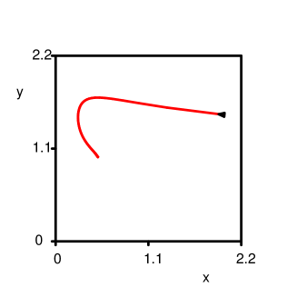
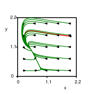
Figure 5.1: A trajectory starting at point $x(0)=2,y(0)=1.5$ (a) and the complete phase portrait of system (5.3) generated by a computer

The main aim of our course is to develop the procedure of drawing a phase portrait of a general system of two non-linear differential equations without using a computer. We expect that as for 1D differential equation (section 3.2.1) and for 2D linear systems (section 4.1) the phase portrait should include two main elements: equilibria points and flows (trajectories) between them. Let us define first equilibria points of a general non-linear system (5.1).

5.1.2 Equilibria

In the 1D case and for 2D linear systems the equilibria were the points where our system is stationary: placed at equilibrium point the system will stay there forever. Therefore, for 1D equation ${dx\over dt}=f(x)$ equilibria were determined as the points where ${dx\over dt}=0$, i.e. where $f(x)=0$. For 2D linear system (section 4.1) we required that both variables $x$ and $y$ are stationary at equilibria points, i.e. both ${dx\over dt}=0$ and ${dy\over dt}=0$. For a general non-linear system (5.1) these conditions yield the following definition of equilibria:

Definition 7

A point $(x^{*},y^{*})$ is called an equilibrium point of a system (5.1) if

$$f(x^{*},y^{*})=0,\quad g(x^{*},y^{*})=0$$ (5.4)

Equilibria in two dimensions are also stationary points, i.e. if system is placed at the equilibrium it will stay there forever. Thus this trajectory will contain just one point.

Example. Find the equilibria of the system (5.3):

Solution To find the equilibria we need to solve a system of algebraic equations (5.4) which in our case becomes:

$$\left\{\begin{array}[]{l}3x(1-x)-1.5xy=0\\ 0.5xy-0.25y=0\end{array}\right.$$ (5.5)

From the second equation we find $y(0.5x-0.25)=0$, which can be either when $y=0$ or when $x=0.5$. Substitution of $y=0$ to the first equation yields $3x(1-x)-0=0$. This equation has two solutions $x=0$ and $x=1$. Substitution of the other case $x=0.5$ to the first equation gives $3*0.5*(1-0.5)-1.5*0.5y=0$, or $y=1$. Thus we have found three equilibria points: $(0,0),(1,0)$ and $(0.5,1)$.

We see in fig.5.1 that point $(0.5,1)$ is indeed an important attractor of our system which determines the final state of the populations. The other two points are not apparent in fig.5.1, however, as we will see later they also account for important changes of trajectories of our system.

Thus we have defined equilibria for 2D systems. Our next step is to understand what is the 2D analog of flows, which on the 1D phase portrait were represented by the ’$\rightarrow$’ or $\leftarrow$ arrows.

5.1.3 Vector field

In 1D flows, visualizations of the direction of change of the variable $x$ were given via the sign of its derivative ${dx\over dt}$. In 2D, both variables can change and the rate of their change is given by the derivatives ${dx\over dt}$ and ${dy\over dt}$. In 1D we were able to find the direction of flow at any point $x$ from the right hand side function of the equation ${dx\over dt}=f(x)$. Similarly in 2D we can find ${dx\over dt}$ and ${dy\over dt}$ at any point $(x,y)$ from the right hand sides of system (5.1) ( functions $f(x,y)$ and $(g(x,y)$). For example for system (5.3) at a point $x=1,y=1$ we find ${dx\over dt}=f(x,y)=3x-3x^{2}-1.5xy=3-3-1.5=-1.5$, and ${dy\over dt}=g(x,y)=0.5xy-0.25y.=0.5-0.25=0.25.$ However, what do these two numbers show? They tell us that if the size of the prey population $x=1$ and the size of the predator population is $y=1$, then the prey population decreases with the rate of $-1.5$ and the predator population grows with the rate of $0.25$. On the phase plane $x,y$ this will result in a shift of a point representing populations from point (1,1) (point $A$ in fig.5.2a) to some point $B$ which is to the left and upward from point $A$. Let us make it more quantitative. We know that the rate of change of $x$ in our case is $1.5/0.25$ times larger than the rate of change of $y$. This determines the direction of shift of point $B$ relative to point $A$. The easiest way to represent it is to draw from point $(1,1)$ a horizontal arrow heading to the left with the length of $1.5$ and a vertical arrow heading upward with the length of $0.25$. The direction of the overall shift will be given by the resultant vector of these two vectors fig.5.2b. The resultant vector will give us the direction tangent to the trajectory which goes through the given point. We can generalize this result as:

Figure 5.2:

Conclusion 9

At any point $(x,y)$ of a phase space for system (5.1), we can define the vector $\vec{v}$ with the components $(f(x,y),g(x,y))$. Such vectors will be tangent to the trajectories of our system. We can find this vector field without a solution of our system, just from the right hand sides of our system.

Note, that the length of the vector in fig.5.2 is not important, as we are interested in the direction, only. If we apply the same procedure at many points and represent the directions by shorter vectors we will get the following vector field of the system (5.3) (fig.5.3).

Figure 5.3:

We see that although the vector field describes qualitatively the direction of trajectories in the phase portrait of our system, it does not give us information on convergence/divergence of trajectories, thus we cannot determine the attractors of our system, which is crucial for our study. However, as we will see in chapter 6 we can elaborate the vector field based methods and in many cases will be able to obtain convergence/divergence information using the so-called graphical Jacobian approach.

But in order to derive this approach we need to understand how to find attractors of a general non-linear system (5.1) using an analytical approach. For that we need to establish the relation of the general non-linear system (5.1) and the general linear system (4.1) that we studied in chapter 4.

5.2 Linearization of a system: Jacobian

Consider a general system of two differential equations:

$$\left\{\begin{array}[]{l}{dx\over dt}=f(x,y)\\ {dy\over dt}=g(x,y)\end{array}\right.$$ (5.6)

In this section we will show that close to equilibrium point the phase portrait of this general non-linear system (5.6) can be found from the solution of the linear system (4.1) that we studied in chapter 4. As a consequence we will get six possible types of equilibria, that are: saddle, non-stable and stable node, non-stable and stable spiral, and a center.

Our main tool here will be a formula (5.7) for the approximation of function of two variables $f(x,y)$ around point $(x^{*},y^{*})$ which we derived in section 2.4:

$$f(x,y)\approx f(x^{*},y^{*})+(\partial f/\partial x)(x-x^{*})+(\partial f/\partial y)(y-y^{*})$$ (5.7)

where $\partial f/\partial x$ and $\partial f/\partial y$ are the values of the partial derivatives at the point $(x^{*},y^{*})$, i.e. they are just numbers.

We will apply this formula to approximate the functions $f(x,y)$ and $g(x,y)$ of our system (5.6) and later solve the approximated system and find the phase portraits close to the equilibrium.

Let us start the derivation. Assume that system (5.6) has an equilibrium point at ($x^{*},y^{*}$). This means (see (5.4)) that:

$$\left\{\begin{array}[]{l}f(x^{*},y^{*})=0\\ g(x^{*},y^{*})=0\end{array}\right.$$ (5.8)

Let us approximate $f(x,y)$ close to the equilibrium using the formula (5.7):

$$f(x,y)\approx f(x^{*},y^{*})+(\partial f/\partial x)(x-x^{*})+(\partial f/\partial y)(y-y^{*})$$

As we assumed ($x^{*},y^{*}$) is an equilibrium, i.e. $f(x^{*},y^{*})=0$ and we get

$$f(x,y)\approx(\partial f/\partial x)(x-x^{*})+(\partial f/\partial y)(y-y^{*})$$ (5.9)

A similar approach for $g(x,y)$ yields:

$$g(x,y)\approx(\partial g/\partial x)(x-x^{*})+(\partial g/\partial y)(y-y^{*})$$ (5.10)

If we replace the right hand sides of (5.6) by their approximations (5.9), (5.10), we get the following system:

$$\left\{\begin{array}[]{l}{dx\over dt}=(\partial f/\partial x)(x-x^{*})+(\partial f/\partial y)(y-y^{*})\\ {dy\over dt}=(\partial g/\partial x)(x-x^{*})+(\partial g/\partial y)(y-y^{*})\end{array}\right.$$ (5.11)

The system (5.11) is simpler than the original system (5.6), as the partial derivatives in (5.11) are constants (numbers, as they are evaluated at the equilibrium point $x^{*},y^{*}$). So we can rewrite (5.11) as :

$$\left\{\begin{array}[]{l}{dx\over dt}=a(x-x^{*})+b(y-y^{*})\\ {dy\over dt}=c(x-x^{*})+d(y-y^{*})\end{array}\right.$$ (5.12)

where $a=\partial f/\partial x;b=\partial f/\partial y;c=\partial g/\partial x,d=\partial g/\partial y$. We can simplify (5.12) even more. For that let us introduce new variables:

$$u=x-x^{*}\qquad v=y-y^{*}$$ (5.13)

were $u,v$ are new unknown functions of $t$. If we substitute them into the right hand side of (5.12),we get:

$$\left\{\begin{array}[]{l}{dx\over dt}=au+bv\\ {dy\over dt}=cu+dv\end{array}\right.$$ (5.14)

In order to substitute $u$ and $v$ into the left hand side of (5.14), note that $u(t)=x(t)-x^{*}$, i.e. ${du\over dt}={dx\over dt}-0$ (here ${dx^{*}\over dt}=0$ because $x^{*}$ is a constant). Similarly, ${dv\over dt}={dy\over dt}$. After replacing ${dx\over dt}$ by ${du\over dt}$ and ${dy\over dt}$ by ${dv\over dt}$ in (5.14) we get:

$$\left\{\begin{array}[]{l}{du\over dt}=au+bv\\ {dv\over dt}=cu+dv.\end{array}\right.$$ (5.15)

System (5.15) coincides with a general linear system (4.1) that we studied in chapter 4 and for which we found six possible types of solutions resulting in six possible phase portraits: saddle, non-stable and stable node, non-stable and stable spiral, and a center. However, how can we use the results of study of system (5.15) for the study of the original system (5.6)? In order to derive (5.15) we made two steps: (1) we used formula (5.7) for function approximation; (2) we changed variables $x,y$ to $u,v$. Let us analyze each of these two steps. (1) As we discussed earlier, formula (5.7) gives a good approximation of the function $f(x,y)$ only if $x,y$ is close to the point of approximation $x^{*},y^{*}$. So we can use the linear system (5.15) for approximating the solutions of the non-linear system (5.6) only close to the equilibrium point $(x^{*},y^{*})$. (2) about change of variables. Equation (5.13) gives the variables $u,v$ via the variables $x,y$. However, we can also solve the equations and find how $x,y$ will be expressed in terms of $u,v$:

$$x=u+x^{*}\qquad y=v+y^{*}$$ (5.16)

Using this expression we can draw the trajectories for our original variables $x(t),y(t)$ if we know the trajectories $u(t),v(t)$ of the linearized system (5.15). Indeed, as the $x$ coordinate of the trajectory equals $u$ plus number $x^{*}$, and the $y$ coordinate equals $v$ plus number $y^{*}$, the only thing what we need to do is just to draw the trajectory $u(t),v(t)$ and shift its $x$-coordinate by $x^{*}$ and the $y$-coordinate by $y^{*}$ units. As we know in a general linear system (5.15) the phase portrait is centered around a point $(0,0)$, therefore all what we would need to do in order to draw the phase portrait of the non-linear system (5.6) close to its equilibrium $(x^{*},y^{*})$ is just to shift the phase portrait of the linear system (5.15) to a location of equilibrium in non-linear system (5.6). If, for example, the linearized system (5.15) will have a stable node type phase portrait, then a non-linear system (5.6) will have the same stable node point but around an equilibrium $(x^{*},y^{*})$ as shown in fig.5.4.

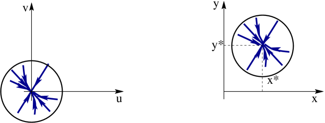
Figure 5.4:

Conclusion 10

The phase portrait of liner system (5.15) close to the origin ($u=0,v=0$) is similar to the phase portrait of non-linear system (5.6) close the to equilibrium point $(x^{*},y^{*})$. To draw the phase portrait of non-linear system (5.6) close to equilibrium, we need to shift a phase portrait of linear system (5.15) from the origin the equilibrium point $(x^{*},y^{*})$.

To find the linearized system (5.15) we need to find the equilibrium point ($x^{*},y^{*}$) and compute the following four numbers: the values of derivatives of right hand sides of our system at this equilibrium:

$$a=\partial f/\partial x\;\;b=\partial f/\partial y\;\;c=\partial g/\partial x\;\;d=\partial g/\partial y$$

So, system (5.15) can be written as:

$$\left\{\begin{array}[]{l}{du\over dt}={\partial f\over\partial x}u+{\partial f\over\partial y}v\\ {dv\over dt}={\partial g\over\partial x}u+{\partial g\over\partial y}v.\end{array}\right.$$ (5.17)

From coefficients of this system we can construct a matrix $J$ that is called the Jacobian

$$J=\left(\begin{array}[]{lr}{\partial f\over\partial x}&{\partial f\over\partial y}\\ {\partial g\over\partial x}&{\partial g\over\partial y}\end{array}\right)$$ (5.18)

Example Find qualitative phase portrait of system (5.3) close to a nontrivial equilibrium point (i.e. at the equilibrium where $x\neq 0,y\neq 0$).

$$\left\{\begin{array}[]{l}{dx\over dt}=3x(1-x)-1.5xy\\ {dy\over dt}=0.5xy-0.25y\end{array}\right.$$

Solution In section 5.1.2 we found that this system has three equilibria $(0,0)$, $(1,0)$, and $(0.5,1)$. The nontrivial equilibrium is $(0.5,1)$. To find the Jacobian of our system we compute the partial derivatives (5.18) and evaluate them at the equilibrium point. In our case $f(x,y)=3x(1-x)-1.5xy;\;g(x,y)=0.5xy-0.25y$.

${\partial f/\partial x}=3-6x-1.5y$ at point $(0.5,1)$ this derivative equals ${\partial f/\partial x}=3-3-1.5=-1.5$. Similarly: ${\partial f/\partial y}=-0.75;\;{\partial g/\partial x}=0.5;\;{\partial g/\partial y}=0$, hence the linearization of our system at point $(0.5,1)$ is

$$\left\{\begin{array}[]{l}{du\over dt}=-1.5u-0.75v\\ {dv\over dt}=0.5u\end{array}\right.$$

or the Jacobian is:

$$J=\left(\begin{array}[]{lr}-1.5&-0.75\\ 0.5&0\end{array}\right).$$

In order to find a phase portrait of this linear system we need to find eigen values of the Jacobian matrix from the following characteristic equation (2.31):

$$Det\left|\begin{array}[]{lr}-1.5-\lambda&-0.75\\ 0.5&0-\lambda\end{array}\right|=(-1.5-\lambda)(-\lambda)+0.5*0.75$$

$$=\lambda^{2}+1.5\lambda+0.375=0$$

Using ’abc’ formula we find that:

$$\lambda_{12}={-1.5\pm\sqrt{2.25-1.5}\over 2}={-1.5\pm\sqrt{0.87}\over 2}$$ (5.20)

or, $\lambda_{1}=-1.36$ and $\lambda_{1}=-0.138$. Because both eigen values are real and negative we will have a stable node and a phase portrait qualitatively similar to that in fig.5.4b.

5.3 Determinant-trace method for finding the type of equilibrium

In this section we derive a simple method for finding signs of eigen values and the type of equilibrium of the linear system (4.1). The results will also be applicable for a general non-linear system (5.6), because, as discussed in the previous section, the equilibrium type of a non-linear system can be found from its linearization.

The eigen values of system (4.1) are the roots of the characteristic equation (2.31):

$$Det\left|\begin{array}[]{lr}a-\lambda&b\\ c&d-\lambda\end{array}\right|=0,$$ (5.21)

or:

$Det\left|\begin{array}[]{lr}a-\lambda&b\\ c&d-\lambda\end{array}\right|=(a-\lambda)(d-\lambda)-cb={\lambda}^{2}-\lambda(a+d)+ad-cb=0$

Let us express the last equation in a slightly different form using the following definition:

Definition 8

The trace of the matrix $\left(\begin{array}[]{lr}a&b\\ c&d\end{array}\right)$ is $trA=a+d$.

The determinant of the matrix $A$ is $detA=ad-cb$

So we can rewrite the characteristic equation using the definition of the trace and the determinant as follows:

$${\lambda}^{2}-trA\lambda+detA=0$$ (5.22)

We see that although the original system depends on four parameters $a,b,c,d$ the characteristic equation depends only on two parameters $trA$ and $detA$, thus if we know the determinant and the trace of our system we can find the eigen values and the type of the equilibrium of the system. Indeed, from (5.22) we can easily find that the eigen values are:

$$\lambda_{1,2}={trA\pm\sqrt{D}\over 2}\quad where\quad D=(trA)^{2}-4detA$$ (5.23)

Roots of the equation (5.23) are as the roots of any quadratic equation, connected in the following way to the coefficients of the equation:

$$\lambda_{1}+\lambda_{2}=trA$$ (5.24)

$$\lambda_{1}*\lambda_{2}=detA$$ (5.25)

To prove the properties (5.24) and (5.25), just note that if $\lambda_{1}$ and $\lambda_{2}$ are the roots of a quadratic (5.22), then it can be written as: ${\lambda}^{2}-trA\lambda+detA=(\lambda-\lambda_{1})((\lambda-\lambda_{2})$. The direct computation yields:

$$\begin{array}[]{l}{\lambda}^{2}-trA\lambda+detA=(\lambda-\lambda_{1})((\lambda-\lambda_{2})\\ or\\ {\lambda}^{2}-trA\lambda+detA=\lambda^{2}-\lambda_{1}\lambda-\lambda_{2}\lambda+\lambda_{1}\lambda_{2}\\ or\\ {\lambda}^{2}-trA\lambda+detA=\lambda^{2}-(\lambda_{1}+\lambda_{2})\lambda+\lambda_{1}\lambda_{2}\end{array}$$

If we now compare the left and the right hand sides of the last equation we will get both properties (5.24) and (5.25).

Let us start classification.

1. If $detA<0$, then $D=(trA)^{2}-4detA>0$, so we have real roots. From (5.25) we conclude that their product is negative, i.e. roots have different signs, i.e. $\lambda_{1}<0,\lambda_{2}>0$, or $\lambda_{1}>0,\lambda_{2}<0$ and we have a saddle point.

2. If $detA>0$, then $D=(trA)^{2}-4detA$ can be negative as well as positive. This means the roots can be real, or complex. Let us consider the case of real roots first, i.e.

   $$D=(trA)^{2}-4detA\geq 0$$ (5.26)

   If (5.26) holds, the roots are real. Next, let us use the property $\lambda_{1}*\lambda_{2}=detA$. In the case of $detA>0$, the product of the roots is positive, i.e. the roots have the same sign. They can be both positive, or both negative. The sign of the roots can be found from the trace of the matrix ($\lambda_{1}+\lambda_{2}=trA$). When $trA>0$, then $\lambda_{1}>0$, and $\lambda_{2}>0$ and we have a non-stable node. When $trA<0$, $\lambda_{1}<0$ and $\lambda_{2}<0$ and we have a stable node. Let us formulate it as a separate case:

3. If $detA>0$, $D>0$ and $trA<0$ the equilibrium is a stable node.

   Let us put this information into a graph (fig.5.5). On this graph let us use $trA$ as the $x$-axis and $detA$ as the $y$-axis. Case 1 of a saddle point then corresponds to the lower half plane (region 1). The line (5.26), which separates real and complex roots, is the parabola given by $detA=(trA)^{2}/4$, or $y=x^{2}/4$. Real roots are below this line. Therefore, in region 2, where $trA>0$, we have case 2 of a non-stable node. In region 3 $trA<0$ and we have case 3 of a stable node.

4. If $detA>0$, and $D<0$, we have complex roots. In accordance with (5.24) and (4.27) they are:

   $$\lambda_{1,2}={trA\over 2}\pm i{\sqrt{-D}\over 2}$$

   Hence, $Re\lambda_{1,2}={trA/2}$. From this we immediately see that if $trA>0$, we have a non-stable spiral (region 4).

5. If $detA>0$, $D<0$ and $trA<0$, we have a stable spiral (region 5).

6. The last case of a center point appears when $Re\lambda_{1,2}={trA/2}=0$, or when $trA=0$ and $detA>0$. In our graph is it the upper part of the $detA$ axis (region 6)

Figure 5.5:

Let us apply this method for several examples:

Example. Find the equilibrium type for the following systems:

a)$\left(\begin{array}[]{c}{dx\over dt}\\ {dy\over dt}\end{array}\right)=\;\left(\begin{array}[]{lr}1&2\\ 3&4\end{array}\right)\left(\begin{array}[]{c}x\\ y\end{array}\right);\quad$    b)$\left(\begin{array}[]{c}{dx\over dt}\\ {dy\over dt}\end{array}\right)=\;\left(\begin{array}[]{lr}4&1\\ 1&2\end{array}\right)\left(\begin{array}[]{c}x\\ y\end{array}\right);\quad$
c)$\left(\begin{array}[]{c}{dx\over dt}\\ {dy\over dt}\end{array}\right)=\left(\begin{array}[]{lr}-2&3\\ -2&1\end{array}\right)\left(\begin{array}[]{c}x\\ y\end{array}\right);\quad$ d)$\left(\begin{array}[]{c}{dx\over dt}\\ {dy\over dt}\end{array}\right)=\left(\begin{array}[]{lr}1&-1\\ 2&-1\end{array}\right)\left(\begin{array}[]{c}x\\ y\end{array}\right);\quad$

Solution Our plan is to find $detA,trA$ for the corresponding matrices and make a conclusion.

a) The matrix is $A=\left(\begin{array}[]{lr}1&2\\ 3&4\end{array}\right);\;trA=1+4=5;\;detA=1*4-2*3=-2$. Therefore we have case 1, hence the system has a saddle point.

b) The corresponding matrix is $A=\left(\begin{array}[]{lr}4&1\\ 1&2\end{array}\right);\;trA=4+2=6;\;detA=4*2-1*1=7$. As $detA>0$ we need to check that the roots are real. We have $D=(trA)^{2}-4detA=6*6-4*7=36-28>0$, hence the roots are real and we have case 2, hence the system has a non-stable node.

c) $trA=-2+1=-1;\;detA=-2+6=4;\;D=(trA)^{2}-4detA=1-4*4=-15<0$, we have complex roots and we are in region 5 and have a stable spiral

d) $trA=1-1=0;\;detA=-1+2=1$, so we have case 6 and we have a center point, or oscillation in our system.

5.4 Exercises

Exercises sec.5.1

1. (A) Find equilibria of the following systems $\left\{\begin{array}[]{l}{dx\over dt}=f(x,y)\\ {dy\over dt}=g(x,y)\end{array}\right.$ (see definition in section 5.1.2).
   (B) Find the following partial derivatives at each equilibrium point (${\partial f\over\partial x},{\partial f\over\partial y},{\partial g\over\partial x},{\partial g\over\partial y}$).
   (a) $\left\{\begin{array}[]{l}{dx\over dt}=-4y\\ {dy\over dt}=4x-x^{2}-0.5y\end{array}\right.$ (b) $\left\{\begin{array}[]{l}{dx\over dt}=9x+y^{2}\\ {dy\over dt}=x-y\end{array}\right.$

   (c) $\left\{\begin{array}[]{l}{dx\over dt}=2x-xy\\ {dy\over dt}=-y+y^{2}x\end{array}\right.$ (d) $\left\{\begin{array}[]{l}{dx\over dt}=(1-x-3y)x\\ {dy\over dt}=(1-2x-2y)y\end{array}\right.$

   (Hint: See an example of solution in section 11.0.2).

2. Find equilibria of the following Lotka Volterra model with competition in the prey population. Determine for which parameter values all equilibria are non-negative.

   $$\left\{\begin{array}[]{l}dN/dt=aN-eN^{2}-bNP\\ dP/dt=cNP-dP\;\;\;\;\;\;\;a,b,c,d,e>0\end{array}\right.$$

3. Protein synthesis depends on DNA transcription ($a$) making mRNA molecules ($M$) and translation ($c$) of mRNA into proteins ($P$). Some proteins inhibit the transcription of their own mRNA ($\frac{1}{1+P}$). mRNA and proteins are degraded at rates b and d, respectively. This process gives the following of two differential equations. Find equilibria of this model.

   $$\left\{\begin{array}[]{l}dM/dt={a\over 1+P}-bM\;\;P,M\geq 0\\ dP/dt=cM-dP\;\;\;\;\;\;\;a,b,c,d>0\end{array}\right.$$

4. Mathematical epidemiology also makes use of simple ODE models. One of these models describes the number of susceptible individuals ($S$) and infected individuals ($I$). Individuals are born at rate ($B$), and die at rate ($\mu$). Susceptible individuals can become infected when they come into contact with infected individuals ($-\beta SI$). Once infected, an individual has a certain death rate ($\alpha$); this may be different from the death rate of non-infected individuals. This process can therefore be modeled by the following equations: $\left\{\begin{array}[]{l}dS/dt=B-\beta SI-\mu S\\ dI/dt=\beta SI-\alpha I\;\;\;\;\;\;\;B,\alpha,\beta,\mu>0\end{array}\right.$
   Find equilibria of this model. Determine for which parameter values all equilibria are non-negative.

   Exercises sec. 5.2 and 5.3

5. Find the type of equilibria using the $det$-$tr$ method. Determine the stability of the equilibrium.
   (a) $\left\{\begin{array}[]{l}{dx\over dt}=3x+y\\ {dy\over dt}=-20x+6y\end{array}\right.$ (b) $\left\{\begin{array}[]{l}{dx\over dt}=2x+y\\ {dy\over dt}=2x-10y\end{array}\right.$ (c) $\left\{\begin{array}[]{l}{dx\over dt}=2x+y\\ {dy\over dt}=5x-2y\end{array}\right.$ (d) $\left\{\begin{array}[]{l}{dx\over dt}=x+10y\\ {dy\over dt}=-10x-y\end{array}\right.$

6. Consider the following model for the algae population: $\left\{\begin{array}[]{l}{dx\over dt}=2x(1-y)\;\;x\geq 0;\\ {dy\over dt}=2-y-x^{2}\;\;y\geq 0.\end{array}\right.$

   1. Find equilibria

   2. Find the general expression for the Jacobian of this system

   3. Determine type of each equilibrium using $det$-$tr$ method

   4. Draw qualitative local phase portraits around each equilibrium point

7. Consider the following biological model:

   $$\left\{\begin{array}[]{l}de/dt=b*e-e^{3}-g\\ dg/dt=e-g\;\;\;b\geq 0\end{array}\right.$$ (5.27)

   • For which values of parameter $b$ the system has only one equilibrium?

   • Determine stability and type of this equilibrium in found parameter range (in which system (5.27) has only one equilibrium).

8. Study the Lotka-Volterra model for a predator-prey system: $\left\{\begin{array}[]{l}{dN\over dt}=aN-bNP\\ {dP\over dt}=cNP-dP\end{array}\right.$
   here $N$ denotes the prey population, $P$ denotes the predator population and $a>0,b>0,c>0,d>0$ are parameters

   1. Find the nontrivial equilibrium of the system (i.e. an equilibrium where $N\neq 0,P\neq 0$).

   2. Find the linearization of the system at this point (i.e. the Jacobian matrix)

   3. Determine the type of the equilibrium

   4. Sketch the phase portrait around this equilibrium. Which kind of dynamics do we expect here?

   Additional exercises

9. Consider the system: ${dx\over dt}=x+4y+e^{x}-1;{dy\over dt}=-y-y*e^{x}$

   1. Check that ($0,0$) is an equilibrium point of the system

   2. Find the general expression for the Jacobian of this system

   3. Find the Jacobian at the point ($0,0$)

   4. Write the linearization of the system close to the equilibrium ($0,0$)

10. Find the equilibria of the following systems. Compute the Jacobian at the equilibria points. Determine type of each equilibrium using $det$-$tr$ method. Draw qualitative local phase portraits around each equilibrium point.
    (a)$\left\{\begin{array}[]{l}{dx\over dt}=y^{2}-3x+2\\ {dy\over dt}=x^{2}-y^{2}\end{array}\right.$ (b) $\left\{\begin{array}[]{l}{dx\over dt}=y\\ {dy\over dt}=-x+x^{3}\end{array}\right.$

11. Revisit solutions of problems 1. Use found equilibria and partial derivatives at these equilibria points to determine type of each equilibrium using $det$-$tr$ method. Draw qualitative local phase portraits around each equilibrium point.

12. Consider a modification of the Lotka-Volterra model, which includes competition in the prey population ($-eN^{2}$): $\left\{\begin{array}[]{l}{dN\over dt}=aN-eN^{2}-bNP\\ {dP\over dt}=cNP-dP\end{array}\right.$, where the parameters $a,b,c,d,e>0$ and the variables $N\geq 0$, $P\geq 0$.

    1. Find all equilibria of this system.

    2. Compute the Jacobian at each equilibrium point.

    3. At which parameter values do we have a non-trivial equilibrium (i.e. an equilibrium at which both $N$ and $P$ are positive). Find stability of this equilibrium.

13. Consider the following model for cardiac tissue:

    $$\left\{\begin{array}[]{l}de/dt=-e(e-a)(e-1)-g\qquad 0<a<1\\ dg/dt=\varepsilon e\qquad\varepsilon>0\end{array}\right.$$ (5.28)

    Here the variable $e$ accounts for the transmembrane potential, the variable $g$ accounts for the refractory period and $a,\varepsilon$ are the parameters.

    The shape of the action potential in cardiac tissue is an important characteristic of myocardium. If the recovery of the transmembrane potential shows oscillation as in fig.5.6b. it can cause dangerous cardiac arrhythmias. From a mathematical point of view the oscillations in fig5.6b occur when system (5.28) has an equilibrium point which is a stable spiral. Monotonous recovery occurs when this equilibrium is a stable node.

    

    Figure 5.6: The monotonous (a) and oscillatory recovery (b) in an excitable medium

    Determine for which parameter values we will have situation fig.5.6a and for which parameter values we will have situation fig.5.6b.

Chapter 6 Graphical methods to study systems of differential equations

In the first section of this chapter we will start from the vector field of a general non-linear system introduced in section 5.1.3, and find how we can approximate the vector field by the so-called null-cline method, without using a computer. Then, in section 6.2, we will show that the null-clines can be used not only for vector field approximation but also for determining the type of an equilibrium point without explicit computation of the Jacobian of the system.

6.1 Null-clines

We introduced the vector field in section 5.1.3, where we showed that for a general 2D system

$$\left\{\begin{array}[]{l}{dx\over dt}=f(x,y)\\ {dy\over dt}=g(x,y)\end{array}\right.$$ (6.1)

the direction of the trajectories on the phase portrait will be along the vector $\vec{v}$ with the components $(f(x,y),g(x,y))$. Thus, to draw the vector field of a particular system we need to evaluate the values of the functions $(f(x,y),g(x,y))$ in many points which usually requires using a computer. In this section we will develop a so-called method of null-clines, which will allow us to sketch a qualitative picture of the vector field analytically. The main idea here is similar to what we did in the 1D case, where we have represented the derivative ${dx\over dt}$ by arrows of two types: ’$\rightarrow$’ for ${dx\over dt}>0$ and ’$\leftarrow$’ for ${dx\over dt}<0$. In 2D the vector field has two components $V=(v_{x},v_{y})=({dx\over dt},{dy\over dt})$. Each of these components ${dx\over dt},{dy\over dt}$ can be positive, or negative. Therefore, we can have the following four cases shown fig.6.1. (Note, that we use different line types there that will be important in the future).

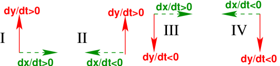
Figure 6.1:

The method of null-clines represents the vector field using these four cases. The main idea behind this method is the following. If we compare cases I and II we see that they differ by the sign of the ${dx\over dt}$ derivative: for case I ${dx\over dt}>0$ and for case II ${dx\over dt}<0$. Therefore these cases are separated by the boundary where ${dx\over dt}=0$ (fig.6.2a). We know that for system (6.1) ${dx\over dt}=f(x,y)$, therefore the boundary between cases I and II is given by the condition

$$f(x,y)=0$$ (6.2)

Figure 6.2:

Geometrically equation (6.2) gives a graph of one or more lines in the $Oxy$-plane (see section 1.4). Note that at this line the horizontal component of the vector field is zero, therefore the vector is vertical.

Similarly, the transition from case I to case III occurs when ${dy\over dt}=0$ (fig.6.2b). As we know for the system (6.1) ${dy\over dt}=g(x,y)$, hence the separation line in this case is given by the equation:

$$g(x,y)=0$$ (6.3)

and the direction of the vector field at this line is horizontal.

Equation (6.3) will give us not only the boundary between cases I and III but also a boundary between cases II and IV, as the transition between cases II and IV also occurs when ${dy\over dt}=0$. In general equations (6.2),(6.3) give two (or more) lines on the $Oxy$-plane, which separate the plane into several regions with different directions of vectors (cases I-IV).

These lines are called null-clines.

Definition 9

The $x$-null-cline (or ${dx\over dt}=0$ null-cline) is the set of points satisfying the condition $f(x,y)=0$. The $y$-null-cline (or ${dy\over dt}=0$ null-cline) is the set of points satisfying the condition $g(x,y)=0$.

To use the method of null-clines it is useful to note that at the $x$-null-cline the $x$-component of the vector changes its sign, and at the $y$-null-cline the $y$-component of the vector changes its sign. To use this rule effectively we will always denote the vector field components using lines of different types: the horizontal component as a dashed line and the vertical component as a solid line. Let us use these ideas and formulate a plan for finding the vector field using null-clines.

Plan of null-cline analysis for system (6.1)

We assume that on the $Oxy$-plane the $x$-axis is the horizontal axis and the $y$-axis is the vertical axis.

1. Draw ${dx\over dt}=0$ null-clines from the equation $f(x,y)=0$ using a dashed line and ${dy\over dt}=0$ null-clines from the equation $g(x,y)=0$ using a solid line.

2. Choose a point in one of the regions in the $x,y$ plane and find the $x$ and the $y$ -components of the vector field. Use the dashed line for the $x$ component and the solid line for the $y$ component. For finding the directions use the following rule: if $f(x,y)>0$ the $x$ component is directed as ’$\rightarrow$’, if $f(x,y)<0$ it is directed as ’$\leftarrow$’; if $g(x,y)>0$ the $y$-component is directed as $\uparrow$, $g(x,y)<0$ it is directed as $\downarrow$.

3. Find the vector field in the adjacent regions using the following rule:

   1. change the direction of the dashed component of the vector field if in order to get to the adjacent region you cross the dashed null-cline

   2. change the direction of the solid component of the vector field if in order to get to the adjacent region you cross the solid null-cline

   3. show the direction of the vector field on the null-clines.

Note, that instead of dashed and solid lines you can use lines of different colors. Then the last step of this plan would be: change the direction of the component of the same color as the color of the null-cline which we cross to get to the adjacent region.

Note, that although this plan works good in most of cases, there are some situations when components of the vector field do not change their sign at the corresponding null-cline. These are special so-called degenerate cases (exceptions). We will not consider them in our course.

Example Find the vector field of the following system using null-clines.

$$\left\{\begin{array}[]{l}{dx\over dt}=3x(1-x)-1.5xy\\ {dy\over dt}=0.5xy-0.25y\end{array}\right.$$ (6.4)

Solution. We follow our plan as follows

1. The ${dx\over dt}=0$ null-clines are given by the equation $f(x,y)=0$, i.e. $3x(1-x)-1.5xy=x(3-3x-1.5y)=0$. This equation has two solutions: $x=0$ (the vertical line which coincides with the $y$-axis) and $y=2-2x$ which is a straight line with the negative slope $-2$ which goes through the point $(2,0)$. The graphs are shown using dashed lines in fig.6.3. The ${dy\over dt}=0$ null-clines are given by the equation $g(x,y)=0$, i.e. $0.5xy-0.25y=y(0.5x-0.25)=0$, which also has two solutions: $y=0$ (horizontal line which coincides with the $x$-axis) and $x=0.5$ (vertical line through the point $x=0.5$). Graphs are shown by solid lines in fig.6.3.

2. We find that at point $(2,2)$ ${dx\over dt}=3*2*(1-2)-1.5*2*2=-12<0$ and ${dy\over dt}=0.5*2*2-0.25*2=1>0$, hence the direction of the dashed arrow is to the left ’$\leftarrow$’ and of the solid arrow is upward $\uparrow$.

3. Now we complete the picture. For example, to get into the region to the left from point ($2,2$) we cross the solid line, thus we change the direction of the solid component here. Similarly for the other regions. We get the picture as in fig.6.3. Finally we show the vector field on the null-clines.

Figure 6.3:

We see that the vector field in fig.6.3 is a good approximation of the flow in fig.5.3. We also see that attractor ($0.5,1$) is a special point in fig.6.3: the point of intersection of the $x$ and $y$ null-clines. This is not a coincidence. If we compare the conditions for finding the equilibrium point (5.4) and equations for null clines (6.2), (6.3), we see that the first equation for finding equilibria $f(x,y)=0$ is also the equation for $x$ null-cline and the second equation for finding the equilibrium point $g(x,y)=0$, is the equation for the $y$-null-cline. Thus, the solution of system (5.4), which gives the points satisfying both equations, gives the points which belong to both null-clines, i.e. the points of intersection of the null-clines. So we found that:

Conclusion 11

Equilibria are the points of intersection of the $x$ and $y$-null-clines.

Note that this definition applies points of intersection of different null-clines only. For example intersection of null clines of the same type in fig.6.3 at points (0.5,0) and (0,2) do not give equilibria of system (5.3), while intersection of the different null-clines at points (0,0),(1,0), (0.5,1) give the equilibria of this system.

Our next step will be to study how can we apply the null-clines for finding the types of equilibrium.

6.2 Graphical Jacobian

The method which we present here allows, in a number of cases, to find the type of an equilibrium from the null-clines of the system, i.e., even without computation of partial derivatives of the Jacobian in the equilibrium. The main idea behind this method can be seen from the scheme in Fig.6.4. Let us consider an equilibrium point $(x^{*},y^{*})$ and two close points: one located to the right, with the coordinates $(x^{*}+h,y^{*})$, the other upward with the coordinates $(x^{*},y^{*}+h)$. Because we assume that $(x^{*},y^{*})$ is an equilibrium point, $f(x^{*},y^{*})=$ and $g(x^{*},y^{*})=0$ (see (5.4)). We can approximate the partial derivative ${\partial f\over\partial x}$ at $(x^{*},y^{*})$ using a formula similar to (1.9) as : ${\partial f\over\partial x}\approx{f(x^{*}+h,y^{*})-f(x^{*},y^{*})\over h}$, but because $f(x^{*},y^{*})=0$, we get ${\partial f\over\partial x}\approx{f(x^{*}+h,y^{*})\over h}$. If we apply the same approach for all derivatives constituting the Jacobian at the equilibrium point $(x^{*},y^{*})$ we get:

$$J=\left(\begin{array}[]{lr}{\partial f\over\partial x}\approx{f(x^{*}+h,y^{*})\over h}&{\partial f\over\partial y}\approx{f(x^{*},y^{*}+h)\over h}\\ {\partial g\over\partial x}\approx{g(x^{*}+h,y^{*})\over h}&{\partial g\over\partial y}\approx{g(x^{*},y^{*}+h)\over h}\end{array}\right)$$ (6.5)

This approximation will be better if points $(x^{*}+h,y^{*})$ and $(x^{*},y^{*}+h)$ are closer to the equilibrium point, i.e., if $h$ is small. It turns out that in many cases the exact values of the derivative will not be important for us and we will be able to find the equilibrium type from just the sign of the components of the Jacobian. From (6.5) it is clear that the sign of the Jacobian components is the same as the sign of the functions at the appropriate points, e.g. the sign of ${\partial f\over\partial x}$ is the same as the sign of $f(x^{*}+h,y^{*})$, etc. Let us now recall, that the sign of the functions $f(x,y),g(x,y)$ is represented on the vector field of our system. In fact, ’$\rightarrow$’ means that ${dx\over dt}>0$ and occurs at the points where $f(x,y)>0$, the ’$\uparrow$’ means that ${dy\over dt}>0$ and occurs at the points where $g(x,y)>0$ (see fig.6.2), etc. Thus from the vector field we can easily determine the sign of the components of the Jacobian matrix. For example, the negative direction of the $x$-component in fig.6.4a will mean that $f(x^{*}+h,y^{*})<0$ and hence ${\partial f\over\partial x}<0$, the positive direction of the $y$-component in fig.6.4a will mean that $g(x^{*}+h,y^{*})>0$ and thus ${\partial g\over\partial x}>0$. Similarly, in Fig.6.4b the vector field at point $(x^{*}+h,y^{*})$ is vertical, thus ${\partial g\over\partial x}>0$ and ${\partial f\over\partial x}=0$.

Figure 6.4:

We will formulate this result as the following conclusion:

Conclusion 12

The sign of the $x$ and $y$ vector field components to the right from the equilibrium point give the sign of ${\partial f\over\partial x}$ and ${\partial g\over\partial x}$ components of the Jacobian. The sign of the $x$ and $y$ vector field components upward from the equilibrium point give the sign of ${\partial f\over\partial y}$ and ${\partial g\over\partial y}$ components of the Jacobian matrix $J=\left(\begin{array}[]{lr}{\partial f\over\partial x}&{\partial f\over\partial y}\\ {\partial g\over\partial x}&{\partial g\over\partial y}\end{array}\right)$ at this equilibrium point (fig.6.4c).

Three notes on the application of this rule:

• The testing points must be exactly horizontal $(x^{*}+h,y^{*})$ and exactly vertical $(x^{*},y^{*}+h)$ with respect to the equilibrium point.

• Testing points should be as close as possible to the equilibrium and should never cross a null cline when going from the equilibrium. (Putting the testing point to the right from the dashed line in fig.6.4a will be wrong).

• If a null cline is exactly horizontal or exactly vertical then one of the corresponding derivatives will be zero. ( In fig.6.4b,${\partial f\over\partial x}=0;{\partial g\over\partial x}>0$ ).

  

  
  

  Figure 6.5:

Examples. Let us consider several examples of the application of this graphical approach for null-clines presented in Fig.6.5 and Fig.6.6. On all these figures the testing points are marked by filled circles.

From fig.6.5a we find the following components of the Jacobian: $J=\left(\begin{array}[]{lr}-\alpha&-\beta\\ +\gamma&-\delta\end{array}\right)$, where $\alpha,\beta,\gamma,\delta$ stand for unknown positive numbers. Thus we see that $detJ=\alpha\delta+\beta\gamma>0$, and $trJ=-\alpha-\delta<0$, thus (see fig.5.5) we have a stable equilibrium (stable node or stable spiral). On the basis of these data we cannot say whether this equilibrium is a node or a spiral as we cannot compute whether the discriminant of the Jacobian is positive or negative, as this depends on the exact values of the partial derivatives.

From fig.6.5b we find: $J=\left(\begin{array}[]{lr}-\alpha&0\\ 0&-\delta\end{array}\right)$. Thus $detJ=\alpha\delta>0$, $trJ=-\alpha-\delta<0$ and $D=tr^{2}-4Det=(\alpha+\delta)^{2}-4\alpha\delta=\alpha^{2}+2\alpha\delta+\delta^{2}-4\alpha\delta=\alpha^{2}-2\alpha\delta+\delta^{2}=(\alpha-\delta)^{2}>0$, thus we have a stable node.

From fig.6.5c we find: $J=\left(\begin{array}[]{lr}+\alpha&0\\ 0&-\delta\end{array}\right)$. Thus $detJ=-\alpha\delta<0$, and we have a saddle.

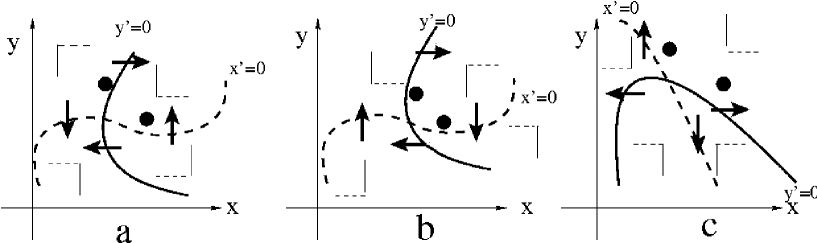
Figure 6.6:

From fig.6.6a we find: $J=\left(\begin{array}[]{lr}+\alpha&+\beta\\ +\gamma&-\delta\end{array}\right)$, hence $detJ=-\alpha\delta-\gamma\beta<0$, and we again have a saddle.

From fig.6.6b we find: $J=\left(\begin{array}[]{lr}+\alpha&+\beta\\ -\gamma&-\delta\end{array}\right)$. $detJ=-\alpha\delta+\gamma\beta$, $trJ=\alpha-\delta$. Because we do not know the values of the coefficients $\alpha,\beta,\gamma,\delta$, just their signs, we do not know if the $detJ$ and $trJ$ are positive or negative, thus we cannot determine the equilibrium type in this case using the graphical Jacobian.

Finally from 6.6c we find: $J=\left(\begin{array}[]{lr}+\alpha&+\beta\\ +\gamma&+\delta\end{array}\right)$. Thus $detJ=\alpha\delta-\gamma\beta$, $trJ=\alpha+\delta>0$. Again we cannot determine the sign of the $detJ$, but positive $trJ$ implies that the equilibrium will be unstable. We do not know its type: non-stable node, non-stable spiral and a saddle are all possible.

We see that the method of graphical Jacobian is a useful tool for finding the equilibrium type from the vector field, but sometimes it is not sufficient and we need to know not only the sign but also the values of the Jacobian coefficients.

6.3 Exercises

1. Sketch the phase portraits of the following systems using null-clines. Try to find the type of equilibrium using the graphical Jacobian (section 6.2). If you are unable to find the equilibrium type using the graphical Jacobian, find it using the method of sec.5.3. Sketch a qualitative phase portrait (without computation of eigen values and eigen vectors).

   1. $\left\{\begin{array}[]{l}{dx\over dt}=3x+y\\ {dy\over dt}=-x-y\end{array}\right.$

   2. $\left\{\begin{array}[]{l}{dx\over dt}=x+2y\\ {dy\over dt}=-2x-2y\end{array}\right.$

   3. $\left\{\begin{array}[]{l}{dx\over dt}=y\\ {dy\over dt}=3x\end{array}\right.$

   4. $\left\{\begin{array}[]{l}{dx\over dt}=x-4y\\ {dy\over dt}=x+y\end{array}\right.$

2. The figure below shows the null-clines of three systems of two non-linear differential equations

   

   1. Complete the figures by showing the direction of the vector field in all regions on the plane and on the null-clines.

   2. Mark the equilibria and find their types using the graphical Jacobian (if possible).

3. Algae model using graphical Jacobian (see also problem 6 from section 5.4):

   $$\left\{\begin{array}[]{l}{dx\over dt}=2x(1-y)\;\;x\geq 0;\\ {dy\over dt}=2-y-x^{2}\;\;y\geq 0.\end{array}\right.$$

   1. Sketch the vector field for the Algae system using null-clines.

   2. Find equilibria.

   3. Find the type of each equilibrium using the graphical Jacobian and draw qualitative local phase portraits.

4. Lotka Volterra model using graphical Jacobian (see also problem 8 from section 5.4):

   $$\left\{\begin{array}[]{l}dN/dt=aN-bNP\quad N\geq 0\\ dP/dt=cNP-dP\quad P\geq 0\end{array}\right.\;\;\;\;\;\;\;a,b,c,d,e>0$$

   1. Sketch the vector field of the system using null-clines.

   2. Find equilibria.

   3. Find the type of each equilibrium using the graphical Jacobian and draw qualitative local phase portraits.

   4. Does the vector field change if we change the values of parameters $a,b,c,d$?

   Additional exercises

5. Find the vector fields of these systems using null-clines. Find equilibria. Determine the type of each equilibrium using the graphical Jacobian and draw qualitative local phase portraits.

   1. $\left\{\begin{array}[]{l}{dx\over dt}=x-3y\\ {dy\over dt}=x+y\end{array}\right.$

   2. $\left\{\begin{array}[]{l}{dx\over dt}=y\\ {dy\over dt}=-x\end{array}\right.$

   3. $\left\{\begin{array}[]{l}{dx\over dt}=9x+y^{2}\\ {dy\over dt}=x-y\end{array}\right.$

   4. $\left\{\begin{array}[]{l}{dx\over dt}=y^{2}-x^{2}\\ {dy\over dt}=y-1\end{array}\right.$

Chapter 7 Plan of qualitative analysis and examples

7.1 Plan

Let us now formulate a plan to qualitatively study a system of two differential equations with two variables and consider several examples.

We study the system:

$$\left\{\begin{array}[]{l}{dx\over dt}=f(x,y)\\ {dy\over dt}=g(x,y)\end{array}\right.$$ (7.1)

Our main aim is to plot the phase portrait of this system and then predict its dynamics. Based on methods which we have developed we will do it in two steps:

1. Null-cline analysis

2. Jacobian analysis

Where the Jacobian analysis can be either performed using the determinant-trace method from section 5.3, or using the graphical Jacobian from sec.6.2. Note, that the determinant-trace method always give us a definitive answer, while the graphical Jacobian method sometimes fails. In more details:

Null-cline analysis

We assume that on the $Oxy$-plane the $x$-axis is the horizontal axis and the $y$-axis is the vertical axis.

1. Draw the ${dx\over dt}=0$ null-clines from the equation $f(x,y)=0$ using dashed lines and the ${dy\over dt}=0$ null-clines from the equation $g(x,y)=0$ using solid lines.

2. Choose a point in one of the regions on the $x,y$ plane and find the vector field for the $x$-component. Denote the $x$ component as a dashed ’$\rightarrow$’ if $f(x,y)>0$ and as a dashed ’$\leftarrow$’ if $f(x,y)<0$.

3. Find the vector field for the $y$-component at the same point. Denote the $y$ component as a solid $\uparrow$ if $g(x,y)>0$ and as a solid $\downarrow$ if $g(x,y)<0$

4. Find the vector field in the adjacent regions using the following rule:

   1. change the direction of the dashed component of the vector field if to get to the adjacent region you cross the dashed null-cline.

   2. change the direction of the solid component of the vector field if to get to the adjacent region you cross the solid null-cline.

   3. show the direction of the vector field on the null-clines close to the equilibrium

Jacobian analysis using the determinant-trace method

1. Find equilibria from equations:

   $$\left\{\begin{array}[]{l}f(x,y)=0\\ g(x,y)=0\end{array}\right.$$ (7.2)

2. For each equilibrium $(x^{*},y^{*})$, find the Jacobian at that equilibrium point

   $$J={\left(\begin{array}[]{lr}{\partial f/\partial x}&{\partial f/\partial y}\\ {\partial g/\partial x}&{\partial g/\partial y}\end{array}\right)}_{(x^{*},y^{*})}$$ (7.3)

   Note: Do not forget to substitute $x=x^{*},y=y^{*}$ into the Jacobian.

3. Determine the type of each equilibrium $(x^{*},y^{*})$. For this compute

   $$detJ={\left({\partial f\over\partial x}*{\partial g\over\partial y}-{\partial f\over\partial y}*{\partial g\over\partial x}\right)}_{(x^{*},y^{*})}$$ (7.4)

   $$trJ={\left({\partial f\over\partial x}+{\partial g\over\partial y}\right)}_{(x^{*},y^{*})}$$ (7.5)

   $$D=(trJ)^{2}-4detJ$$ (7.6)

   To find the type of equilibrium use fig.5.5, or the following list:

   1. If $detJ<0$; the point is a saddle point

   2. If $detJ>0,trJ>0,D\geq 0$; the point is a non-stable node

   3. If $detJ>0,trJ<0,D\geq 0$; the point is a stable node

   4. If $detJ>0,trJ>0,D<0$; the point is a non-stable spiral

   5. If $detJ>0,trJ<0,D<0$; the point is a stable spiral

   6. If $detJ>0,trJ=0$; the point is a center

4. Draw local phase portraits using both knowledge on the equilibrium type and the vector fields obtained using null-cline analysis

5. Connect local phase portraits to get the global picture and show attractors and their basins of attraction.

Jacobian analysis using the graphical Jacobian

1. For each equilibrium point (point of intersection of different null-clines) choose two points, one of which is located to the right and the other upward from the equilibrium. Find the components of the Jacobian using the following rule: the sign of the $x$ component of the vector field to the right of the equilibrium point gives the sign of ${\partial f\over\partial x}$ and the sign of the $y$ component of the vector field to the right of the equilibrium point gives the sign of ${\partial g\over\partial x}$. The sign of the $x$ and $y$ vector field components upward of the equilibrium point give the sign of ${\partial f\over\partial y}$ and ${\partial g\over\partial y}$.

2. Note that if one of the components is zero, then the corresponding derivative of the Jacobian will be zero. The latter can happen if at a given equilibrium point one or both null-clines are exactly horizontal or exactly vertical.

3. Try to compute the sign of the determinant and of the trace of the Jacobian and try to identify the type of equilibrium from fig.5.5.

4. If the type of equilibrium cannot be identified, use the analytical determinant-trace method formulated above.

5. Draw local and then global phase portraits of the system and make predictions about its dynamics.

7.2 Examples

Example 1 Study system (5.3), using null-clines and the determinant-trace method.

$$\left\{\begin{array}[]{l}{dx\over dt}=3x(1-x)-1.5xy\\ {dy\over dt}=0.5xy-0.25y\end{array}\right.$$ (7.7)

Solution We have made studies of different aspects of this model throughout the reader, so let us collect the information.

I.Null-cline analysis.

The null-clines of this system are given in fig.6.3. We repeat it here in fig7.1a:

Figure 7.1:

II.Jacobian analysis:

1. Equilibria. In example eq.(5.5) we found that this system has three equilibria points: $(0,0),(1,0)$ and $(0.5,1)$.

2. Jacobian. We compute the Jacobian as: ${\partial f/\partial x}=3-6x-1.5y;\;{\partial f/\partial y}=-1.5x;\;{\partial g/\partial x}=0.5y;\;{\partial g/\partial y}=0.5x-0.25$, thus: $J=\left(\begin{array}[]{lr}3-6x-1.5y&-1.5x\\ 0.5y&0.5x-0.25\end{array}\right)$.

   Let us find equilibria types from the Jacobian.

   At point $(0,0)$ the Jacobian is: $J_{1}=\left(\begin{array}[]{lr}3&0\\ 0&-0.25\end{array}\right)$, $detJ_{1}=3*(-0.25)<0$, thus this is a saddle point.

   At the point $(1,0)$ the Jacobian is: $J_{2}=\left(\begin{array}[]{lr}-3&-1.5\\ 0&0.25\end{array}\right)$, $detJ_{2}=(-3)*0.25<0$, thus this is a saddle point.

   At the point $(0.5,1)$ the Jacobian is: $J_{3}=\left(\begin{array}[]{lr}-1.5&-0.75\\ 0.5&0\end{array}\right)$, $detJ_{3}=(-1.5)*0-0.5*(-0.75)<0.375$, thus we need to find $trJ_{3}=-1.5$ and $D=(-1.5)^{2}-4*0.375=0.75>0$ thus this is a stable node.

3. Local phase portraits are presented in fig.7.1b. From the null-cline analysis we find the approximate locations of the manifolds of the saddle points and the direction of the trajectories around the stable node.

4. Global picture. There are no general rules to draw the global picture. However in the case of fig.7.1b we can expect that the non-stable manifold of the saddle point at $(0,0)$ will end at the other saddle point $(1,0)$, the non-stable manifold of the saddle point $(1,0)$ as well as most of other trajectories should go to the stable node at $(0.5,1)$ as this is the only attractor here. Thus we get the phase portrait presented in fig.7.1c. We see that we will have a stable global attractor with the basin of attraction the whole region $x>0,y>0$ (except two axes $x=0;\;y=0$).

We see that the phase portrait which we got as a result of our study is qualitatively the same as the phase portrait of this system obtained using a computer (see fig.5.1b).

Let us try to apply for this problem the method of the graphical Jacobian

Example 2 Study the same system (7.7), using the graphical Jacobian method.

Solution From fig.7.1a we find in the following components of the Jacobian:

1. Point $(0,0)$, $J=\left(\begin{array}[]{lr}+\alpha&0\\ 0&-\delta\end{array}\right)$. Thus $detJ=-\alpha\delta<0$, thus we have a saddle.

2. Point $(1,0)$, $J=\left(\begin{array}[]{lr}-\alpha&-\beta\\ 0&+\delta\end{array}\right)$. Thus $detJ=-\alpha\delta<0$, thus we have a saddle.

3. Point $(0.5,1)$, $J=\left(\begin{array}[]{lr}-\alpha&-\beta\\ +\gamma&0\end{array}\right)$. Thus $detJ=\gamma\beta>0$, $trJ=-\alpha<0$, thus we have a stable equilibrium (stable node or stable spiral).

4. Drawing of the local and global phase portraits is exactly the same as with the previous method

Thus we see that in this case we were able to solve the problem completely using the graphical Jacobian method. The only difference with the determinant-trace method is that we were not able to say that the stable equilibrium is a node. However, this has almost no consequences for the phase portrait.

7.3 Exercises

1. Complete the vector field approximations for the null-clines shown in fig7.2a,b,c. Mark equilibria and determine their type using the graphical Jacobian method. Draw local and then global phase portraits. Try to describe the dynamics of the system, by saying what happens with the variables $x$ and $y$ in the course of time.

   

   Figure 7.2:

2. Draw the phase portrait of the following systems of differential equations. Explain their dynamics.

   1. $\left\{\begin{array}[]{l}{dx\over dt}=x(1-x-y)\\ {dy\over dt}=y(1-2x)\end{array}\right.x\geq 0;\;y\geq 0$

   2. $\left\{\begin{array}[]{l}{dN\over dt}=2N-NP-N^{2}\\ {dP\over dt}=3P-2NP-P^{2}\end{array}\right.N\geq 0;\;P\geq 0$

3. In theoretical biology the following model has been used to study mRNA ($M$) protein ($P$) interaction:

   $$\left\{\begin{array}[]{l}dP/dt=bM-d_{P}P\;\;\;\;\;\;\;a,b,d>0\\ dM/dt=a{K^{2}b\over K^{2}+P^{2}}-d_{M}M\qquad P>0;M>0\end{array}\right.$$ (7.8)

   Study this system using the graphical Jacobian approach, i.e. draw null-clines, mark equilibria as points of intersection of the null-clines, determine stability of these equilibria and sketch a qualitative phase portrait.

4. The following equations describe the dynamics of predator ($P$) and prey ($N$) populations:

   $$\left\{\begin{array}[]{l}dN/dt=rN(1-{\displaystyle N\over\displaystyle K})-bNP\quad\quad N\geq 0\quad P\geq 0\\ \\ dP/dt=bNP-2bP\quad\quad\quad\quad b\geq 0\;\;K\geq 0\;\;r\geq 0\end{array}\right.$$

   here $K,b,r$ are parameters

   This system of differential equations always has an equilibrium corresponding to an extinct population of the predator and non-zero population of prey ($P=0;N\neq 0$).

   1. Find this ($P=0;N\neq 0$) equilibrium.

   2. Find the Jacobian at this equilibrium point.

   3. For which values of the parameters the predator population can be driven to extinction (i.e. to that equilibrium ).

   (N.B. Do not use the ’graphical Jacobian approach for this problem!).

   Additional exercises

5. Draw the phase portrait of the following systems of differential equations. Explain their dynamics.

   1. $\left\{\begin{array}[]{l}{dx\over dt}=2y\\ {dy\over dt}=x-x^{2}-0.5y\end{array}\right.$

   2. $\left\{\begin{array}[]{l}{dx\over dt}=x+y^{2}\\ {dy\over dt}=x+y\end{array}\right.$

   3. $\left\{\begin{array}[]{l}{dx\over dt}=x(25-x^{2}-y^{2})\\ {dy\over dt}=y(x-3)\end{array}\right.x\geq 0;\;y\geq 0$

   4. $\left\{\begin{array}[]{l}{dx\over dt}=xy\\ {dy\over dt}=4-y-x^{2}\end{array}\right.\quad-\infty<x<\infty;\quad-\infty<y<\infty$

6. Lotka Volterra model with competition in the prey population:

   $$\left\{\begin{array}[]{l}dN/dt=aN-eN^{2}-bNP\\ dP/dt=cNP-dP\end{array}\right.$$

   for $a=3,b=1.5,c=0.5,d=0.25,e=3$.

7. A swimming pool is infested with algae whose population is $N(t)$. The owner attempts to control the infestation with an algicidal chemical, poured into the pool at a constant rate. In the absence of algae, the chemical decays naturally; when algae are present it is metabolized by them and kills them. The equations of the rates of change of $N(t)$ and the concentration of the chemical in the pool, $C(t)$, are

   $$\left\{\begin{array}[]{l}dN/dt=aN-bNC\\ dC/dt=Q-\alpha C-\beta NC\end{array}\right.$$

   where $a,b,Q,\alpha,\beta$ are positive constants. Discuss the meaning of each term in these equations.

   1. Put $a=1,b=1,\alpha=1,\beta=1$ and show, that the system has two non-negative equilibria if $Q>1$, find them, draw the phase portrait of this system and explain the dynamics.

   2. What happens if $Q<1$?

   3. * Find the conditions for control of the infestation for arbitrary positive values of $a,b,Q,\alpha,\beta$.

Chapter 8 Limit cycle

8.1 Stable and non-stable limit cycles

In previous chapters we found several possible types of equilibria: saddle, node, spiral and center. Some of these equilibria can be attractors which determine the ultimate dynamics of a system. However, it turns out that there exists another important attractor for systems of two differential equations. It is called a limit cycle. The geometrical image of a limit cycle on a phase portrait is a closed curve. The usual phase portrait of a system with a limit cycle is shown in fig.8.3a. Here the limit cycle is shown as a bold ellipse. The figure also shows two more trajectories: one inside the limit cycle and one outside the limit cycle. Inside the limit cycle you can see a spiral. This is not unusual. There is a theorem which states that for systems of two equations there is always at least one equilibrium point inside the limit cycle. In most of the cases such an equilibrium point is a spiral. Outside the limit cycle we can see a trajectory which approaches the limit cycle and winds onto it.

The limit cycle which is shown in fig.8.3a is called a stable limit cycle. This is because if we start on a trajectory close to this limit cycle, this trajectory will approach this limit cycle in the course of time.

There also exists another type of limit cycle called a non-stable limit cycle (fig.8.3b). If we start on a trajectory close to a non-stable limit cycle, it will diverge from this limit cycle. In order to distinguish the stable and non-stable limit cycles we will draw the non-stable limit cycle using a dashed line.

The main questions regarding the limit cycle are: what will be the dynamics of systems with limit cycles and how do limit cycles occur in systems of two differential equations? We will also consider an example of a biological system with a limit cycle.

Figure 8.1: Phase portrait of a system of two differential equations with a limit cycle.

Figure 8.2: Dynamics of a system with a stable limit cycle from fig.8.3a.

Figure 8.3: Dynamics of a system with an non-stable limit cycle from fig.8.3b.

8.2 Dynamics of a system with a limit cycle.

What will be the dynamics of systems with a limit cycle? In section 4.4.2 we studied an equilibrium point called a “center”. The phase portrait of that point (fig.4.8) was a set of embedded ellipses. The corresponding dynamics are oscillations of the $x$ and $y$ variables. Therefore, the dynamics which corresponds to the trajectory which starts on the limit cycle will also be oscillations. Fig.8.3a, fig.8.3a shows an example of dynamics of the variable $x$ for the trajectory which starts on the limit cycle (at the point C in fig.8.3).

The dynamics of trajectories originating around the limit cycles will depend on its type. If the limit cycle is stable, then a trajectory which starts inside the limit cycle will approach it in the course of time and we obtain oscillations with initially increasing amplitude (fig.8.3b). If the trajectory starts outside the limit cycle, then we obtain oscillations with an initial decrease of amplitude until the trajectory reaches the limit cycle (fig.8.3c).

For a non-stable limit cycle the dynamics are different. Only the trajectory which starts on a limit cycle will have oscillatory dynamics (fig.8.3a). Other trajectories will have different behavior. The trajectory which originates inside the limit cycle will approach the stable equilibrium inside the limit cycle and we obtain oscillations with gradually decreasing amplitude (fig.8.3b). The trajectory which starts outside the limit cycle blows up to infinity or to another equilibrium (fig.8.3c). The oscillations in fig.8.3a with a non-stable limit cycle are highly improbable in real systems. This is because for such oscillations the trajectory must start exactly on the limit cycle and even small disturbances will switch our system either to the behavior of fig.8.3b or fig.8.3c. Therefore, for real systems the non-stable limit cycle just determines the basin of attraction of the stable equilibrium which is located inside this limit cycle.

8.3 How do limit cycles occur?

In many cases the limit cycle occurs as a result of the changing of a parameter in a system of differential equations. The most usual process of formation of a limit cycle is the following. Assume we have a system of two differential equations with a parameter $c$:

$$\left\{\begin{array}[]{l}{dx\over dt}=f(x,y,c)\\ {dy\over dt}=g(x,y,c)\end{array}\right.$$ (8.1)

Assume that at some parameter value $c=c_{1}$ system (8.1) has a global attractor which is a stable spiral (fig.8.4a). This means that all the trajectories which originate close to or even far from this equilibrium approach it in the course of time. Because our equilibrium point is a stable spiral the Jacobian of the system at this point will have two complex eigen values $\lambda_{1,2}=\alpha\pm i\beta;\alpha<0$. However, because our system will now depend on the parameter $c$ the eigen values will also depend on this parameter:

$$\lambda_{1,2}(c)=\alpha(c)\pm i\beta(c);$$ (8.2)

Because we have assumed that at $c=c_{1}$ system (8.1) has an equilibrium which is a stable spiral, then $\alpha(c_{1})<0$. When we change the parameter $c$ the value of $\alpha(c)$ will change and at some $c_{2}$ it can become a positive number $\alpha(c_{2})>0$. This means that the stable spiral in fig.8.4a will become an unstable spiral. However, as we found in chapter 4 (fig.4.3), the eigenvalues only give us the dynamics close to the equilibrium point of our system. Therefore, it can happen that although close to the equilibrium point our spiral becomes unstable, the global behavior far from the equilibrium remains the same, i.e. far from the equilibrium we still have a converging flow (fig.8.4b). Hence, in our phase portrait we have two types of flow: the diverging flow from the unstable spiral around the equilibrium and the converging flow from the periphery. Simple geometrical consideration shows that these two flows must be separated from each other. The line of separation will be the limit cycle in our system. Therefore, we will obtain a phase portrait as in fig.8.3a.

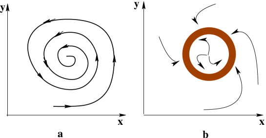
Figure 8.4: Appearance of a limit cycle in a system with a parameter.

Note, that such a mechanism of limit cycle formation frequently occurs in systems of two equations. It is called the Hopf bifurcation. From our analysis it follows that the Hopf bifurcation occurs when $\alpha(c)$ changes its sign, i.e. at the parameter value $c^{*}$ where:

$$\alpha(c^{*})=0$$ (8.3)

8.4 Example of a system with a limit cycle

Let us consider the Holling-Tanner model for predator-prey interactions.

$$\left\{\begin{array}[]{l}dP/dt=rP(1-{P\over K})-{aRP\over d+P}\\ dR/dt=bR(1-{R\over P})\qquad P>0;R>0\end{array}\right.$$ (8.4)

here $P$ denotes the prey and $R$ the predator population, the term $rP(1-P/K)$ describes the growth of the prey in absence of predator, ${aRP\over d+P}$ accounts for the predator-prey interaction. At $a=1,b=0.2,r=1.,d=1.,K=0.7$ system (8.4) has one equilibrium point (for $P>0,R>0$) which is a stable spiral. The null-clines, phase portrait and dynamics of this system are shown in fig.8.5.

Figure 8.5: Dynamics of system (8.4) for $K=0.7$. a-null-clines; b-an orbit; c-time-plot for the both variables for the orbit from fig.b

If we increase the value of the parameter $K$ which accounts for the carrying capacity ($K=1.0$) the type of equilibrium changes and it becomes an unstable spiral. As we discussed in section 8.3 we expect the formation of a stable limit cycle. We can clearly see it in fig.8.6b. The trajectory, which starts from the same initial conditions as the trajectory from fig.8.5b will now approach some closed curve which is a limit cycle and the dynamics of the system will be oscillatory (fig.8.6c).

Figure 8.6: Dynamics of system (8.4) for $K=1.0$. a-null-clines; b-an orbit; c-time-plot for both variables for the orbit from fig.b

Figure 8.7: Dynamics of system (8.4) for $K=1.0$. a-an orbit originating inside the limit cycle; b-time-plot for the both variables for the orbit from fig.a; c-phase portrait of system (8.4)

If we start a trajectory inside the limit cycle then, as we predicted in fig.8.3a and fig.8.3b, the trajectory will approach the limit cycle and the dynamics will be oscillation with increasing amplitude fig.8.7a,b. The complete phase portrait of this system at $K=1$ is shown in fig.8.7c.

You will learn more about the biological consequences of this type of dynamics in the course “Theoretical Biology” by R. de Boer.

Conclusion 13

A limit cycle is a closed trajectory on the phase portrait of a system of two differential equations.

If trajectories around the limit cycle converge onto it, then the limit cycle is called a stable limit cycle. If trajectories around the limit cycle diverge away from it, then the limit cycle is called a non-stable limit cycle.

The dynamics of a system with a stable limit cycle is oscillatory. The dynamics of a system with an non-stable limit cycle is either converging to the equilibrium which is located within the limit cycle or diverging, possibly to infinity.

Limit cycles can appear as a result of a Hopf bifurcation, i.e. the process where the real part of the complex eigenvalues change their sign.

8.5 Exercises

1. Assume that a system of two differential equations has two equilibria which are a saddle point and a non-stable spiral. The phase portrait of this system is partially shown in fig.8.8a What is missing here?

   1. Complete the phase portrait of this system

   2. Qualitatively sketch the dynamics of the variable $x$ ( dependence of the variable $x$ on time) for the initial conditions which are shown in fig.8.8 by the point A in fig.8.8a.

2. Complete the phase portrait of this system shown in fig.8.8b,c. Qualitatively sketch the dynamics of the variable $x$ ( dependence of the variable $x$ on time) for the initial conditions which are shown by points A,B,C in fig.8.8b,c. (Note, that in fig.8.8b,c a stable limit cycle is shown by the solid line and a non-stable limit cycle is shown by the dashed line)

   

   Figure 8.8:

3. As we discussed in (8.3) the necessary condition for the appearance of a limit cycle via a Hopf bifurcation is that the eigenvalues of the Jacobian matrix of a system at the equilibrium point are complex and the real part of the eigenvalues are zero $\alpha(c^{*})=0$. Prove that this condition can be rewritten in the following way using the $det$ and $tr$ of the Jacobian matrix:

   $$trJ(c^{*})=0;\qquad detJ(c^{*})>0$$ (8.5)

4. One of the classical models for oscillatory phenomena in biochemical systems is a model called the Brusselator. In dimensionless form this model can be written as the following system of two differential equations:

   $$\left\{\begin{array}[]{l}{dx\over dt}=a-(b+1)x+x^{2}y\qquad x>0;y>0\\ {dy\over dt}=bx-x^{2}y\qquad a>0;b>0\end{array}\right.$$ (8.6)

   here $x$ and $y$ are concentrations of two biochemical species and $a$ and $b$ are parameters. Study system (8.6) for $a=1$.

   1. Find a non-trivial equilibrium.

   2. Determine the stability of this equilibrium as a function of the parameter $b$.

   3. Find the value of $b$ when system (8.6) undergoes a Hopf bifurcation. (Note: it can be helpful to use equations (8.5)).

   4. For which values of $b$ do you expect oscillations in system (8.6)?

5. Study the following predator-prey model

   $$\left\{\begin{array}[]{l}dP/dt=rP(1-{P\over K})-{aRP\over h+P}\\ dR/dt={caRP\over h+P}-dR\qquad P\geq 0;R\geq 0\end{array}\right.$$ (8.7)

   1. Draw null-clines of this system for $r=1,a=3,h=0.1,c=1.,d=2.5$ and two values of $K$, $K=0.8$ and $K=1.6$. (Hint: the maximum of the parabola $A(x-a)(x-b)$ is reached at the middle between its roots (i.e. at $x={a+b\over 2}$)).

   2. Determine the stability of non-trivial equilibrium in both cases using the graphical Jacobian.

   3. For which value of $K$ do you expect oscillatory behavior?

   4. Extend your analysis for arbitrary positive values of the parameters ($r,a,h,c,d,K>0$) provided $ca>d$. Find for which values of $K$ the non-trivial equilibrium is stable. When do we expect oscillations? (Note, that critical values of $K$ should be a function of the other parameters of the system).

Chapter 9 Historical notes

I developed this course in 1995-2010 for biology students from Utrecht University. The main idea was to develop a course which will allow students with minimal mathematical background to understands basic methods used in mathematical biology. Over the years the course was many times adjusted and modified. The current text contains the latest version of the course from 2010.

Chapter 10 Dictionary

absolute value	absolute waarde
autonomous system	autonoom systeem
attractor	attractor
basin of attraction	basin van attractie
bifurcation	bifurcatie
carrying capacity	draagkracht
center point	centrumpunt
complex conjugate number	complex toegevoegde
component of the vector	component van de vector
determinant	determinant
derivative	afgeleide
differential equation	differentiaal vergelijking
direction field	vectorveld
eigen value	eigenwaarde
eigen vector	eigenvector
equilibrium	evenwicht
general solution	algemene oplossing
harvesting	oogsten
imaginary part of complex number	het imaginaire deel van een complex getal
initial value problem	beginwaarde probleem
Jacobian	Jacobi-matrix
linear approximation	lineaire benadering
modulus	modulus
node	knooppunt
non-stable manifold	instabiele manifold

null-cline	isocline
parameter	parameter
partial derivative	partiële afgeleide
particular solution	specifieke oplossing
phase space	faseruimte
phase portrait	faseplaatje
real part of complex number	het reëele deel van een complex getal
saddle	zadelpunt
spiral	spiraalpunt
stability	stabiliteit
stable manifold	stabiele manifold
system of differential equations	stelsel differentiaal vergelijkingen
trajectory	trajectorie
trace of the matrix	spoor van de matrix
variable	variabele
vector	vector

Chapter 11 Hints:

11.0.1 Solution of the initial value problem for a linear system

Let us illustrate how we can find a solution for the initial value problem, on example of system (4.11).

Problem: Find the solution for the following initial value problem:

$$\left(\begin{array}[]{c}{dx\over dt}\\ {dy\over dt}\end{array}\right)=\left(\begin{array}[]{lr}1&4\\ 1&1\end{array}\right),\quad\left(\begin{array}[]{c}x\\ y\end{array}\right)\left(\begin{array}[]{c}x(0)\\ y(0)\end{array}\right)=\left(\begin{array}[]{c}4\\ 6\end{array}\right)$$ (11.1)

Solution: We already found a general solution of (11.1) as formula (4.20):

$$\left(\begin{array}[]{c}x\\ y\end{array}\right)=C_{1}\left(\begin{array}[]{c}-4\\ 2\end{array}\right)e^{-1*t}+C_{2}\left(\begin{array}[]{c}-4\\ -2\end{array}\right)e^{3*t}$$ (11.2)

Using it we can find a particular solution, corresponding to any given initial conditions.

We proceed as follows. At time $t=0$ (11.2) gives:

$$\left(\begin{array}[]{c}x\\ y\end{array}\right)=C_{1}\left(\begin{array}[]{c}-4\\ 2\end{array}\right)e^{-1*0}+C_{2}\left(\begin{array}[]{c}-4\\ -2\end{array}\right)e^{3*0}=C_{1}\left(\begin{array}[]{c}-4\\ 2\end{array}\right)+C_{2}\left(\begin{array}[]{c}-4\\ -2\end{array}\right).$$

This expression will satisfy the initial conditions if: $C_{1}\left(\begin{array}[]{c}-4\\ 2\end{array}\right)+C_{2}\left(\begin{array}[]{c}-4\\ -2\end{array}\right)=\left(\begin{array}[]{c}4\\ 6\end{array}\right)$. This gives the following system of equations for unknowns $C_{1}$ and $C_{2}$: $\left\{\begin{array}[]{l}-4C_{1}-4C_{2}=4\\ 2C_{1}-2C_{2}=6\end{array}\right.$

We now solve this system using the method described in section 1.1.4. From the second equation we find:
$2C_{1}=6+2C_{2}$, or $C_{1}=3+C_{2}$. After substitution of this expression to the first equation we find:
$-4(3+C_{2})-4C_{2}=4$, i.e. $-12-4C_{2}-4C_{2}=4$, or $-8C_{2}=4+12=16$ and $C_{2}=16/(-8)=-2$.
We now find $C_{1}$ from our substitution as $C_{1}=3+C_{2}=3-2=1$.

Thus $C_{1}=1,C_{2}=-2$ give the solution of our system satisfying given initial conditions. Let us rewrite it as:

$$\left(\begin{array}[]{c}x\\ y\end{array}\right)=1*\left(\begin{array}[]{c}-4\\ 2\end{array}\right)e^{-1*t}-2*\left(\begin{array}[]{c}-4\\ -2\end{array}\right)e^{3*t}=\left(\begin{array}[]{c}-4e^{-1*t}-2*(-4)e^{3*t}\\ 2e^{-1*t}-2*(-2)e^{3*t}\end{array}\right),$$

thus the particular solution is given by $x(t)=-4e^{-1*t}+8e^{3*t}$, and $y(t)=2e^{-1*t}+4e^{3*t}$.

11.0.2 Equilibria/derivatives

Problem:(A) Find equilibria of the following systems $\left\{\begin{array}[]{l}{dx\over dt}=f(x,y)\\ {dy\over dt}=g(x,y)\end{array}\right.$ (see definition in section 5.1.2).
(B) Find the following partial derivatives at each equilibrium point (${\partial f\over\partial x},{\partial f\over\partial y},{\partial g\over\partial x},{\partial g\over\partial y}$).
(a) $\left\{\begin{array}[]{l}{dx\over dt}=4x-2xy\\ {dy\over dt}=2xy-4y\end{array}\right.$

Solution: (A) We rewrite the first equation as $4x-2xy=2x(2-y)=0$. It has solutions $x=0$ or $y=2$.
Let us substitute them to the second equation:
For $x=0$, we get $2*0*y-4y=-4y=0$, thus $y=0$. Therefore we found one equilibrium $x=0,y=0$.
Now substitute $y=2$. We get $2*x*2-4*2=4x-8=0$, thus $x=2$. We found the second equilibrium $x=2,y=2$.

(B) $f(x,y)=4x-2xy$, thus ${\partial f\over\partial x}=4-2y;{\partial f\over\partial y}=-2x$.
$g(x,y)=2xy-4y$, thus ${\partial g\over\partial x}=2y;{\partial g\over\partial y}=2x-4$.
At the equilibiria points:

Equilibrium $x=0,y=0$: ${\partial f\over\partial x}=4-2*0=4;{\partial f\over\partial y}=-2*0=0;{\partial g\over\partial x}=2*0=0;{\partial g\over\partial y}=2*0-4=-4$.

Equilibrium $x=2,y=2$: ${\partial f\over\partial x}=4-2*2=0;{\partial f\over\partial y}=-2*2=-4;{\partial g\over\partial x}=2*2=4;{\partial g\over\partial y}=2*2-4=0$.

Chapter 12 Answers for selected exercises and Formulas lists

Exercises Chapter 1

1. 1. $3axy$

   2. ${6\over r}-{5r\over 30r+5}={-r^{2}+36r+6\over r(6r+1)}$

2. 1. ${\lim_{x\rightarrow\infty}}{ax+q\over c^{2}+x^{2}}=0$

   2. ${\lim_{N\rightarrow\infty}}{aN^{2}+q\over{b\over N}+c^{2}+dN^{2}}={a\over d}$

3. 1. $3r+2-5(r+1)=6r+4$; $r=-{7\over 8}$

   2. $x+{4\over x}=4$; $x_{1,2}=2\pm\sqrt{0}=2$

   3. $(b-{N\over k})N=0$; $N=0$, or $N=bk$.

   4. $N=0$, or $b-d(1+{N\over k})=0$, thus $N={k(b-d)\over d}$.

   5. $N=0$, or $N=h({b\over d}-1)$

4. 1. From 1st eq. $x=2y-5$, substitution to 2nd eq. gives $y=4$, thus $x=3$.

   2. from 1st eq.$x=-{b\over a}y$ to 2nd eq. gives $x=-{b\over a}y=-{b\over a}{-ba\over da-bc}={b^{2}\over da-bc}$

   3. From 2nd eq. $y(4-x)=0$, this $y=0$ or $x=4$. Substitution to the 1st eq. gives or $x=0$ and $x=0.5$. Now substitute $x=4$, we get $y=7$, thus all solutions are given: $(0,0),(0.5,0),(4,7)$.

   4. From 2nd eq. $y(9-3x-y)=0$, thus $y=0$ or $y=9-3x$. Substitution to the 1st eq. gives:
      $(0,0),(4,0),(0,9),(2.5,1.5)$.

   5. From 2nd eq. $N=0$, or $R=\delta$. Substitution to the 1st eq. gives: : $(0,0),(k(1-d),0),(\delta,{1-d\over a}-{\delta\over ak})$.

5. 1. $f^{\prime}(x)={1\over x^{3}}=-{3\over x^{4}}$

   2. $f(x)=e^{-5x}$ and $f^{\prime}(x)=-5e^{-5x}$

   3. $((4x-x^{2})*(2x+3))^{\prime}=10x+12-6x^{2}$

   4. $y^{\prime}={x^{2}+a^{2}\over(a^{2}-x^{2})^{2}}$

6. 1. $y$-intercept $y=-{b\over c^{2}}$, zeros $n=\pm\sqrt{b\over a}$, horizontal asymptote: $y=a$

   2. $y$-intercept $y={hr\over a}$, zeros $R=-h$ and $R=K$.

7. 1. fig.a

   2. fig.b

   3. horizontal asymptote $y=7$, intercept $y(0)=4$. (fig.c). Dependence on $a$. If $a$ increases, the horizontal asymptote $y=7$ will be approached at a slower rate. (fig.c)

      

8. 1. (see below,fig.a)

   2. (see below,fig.b)

      

   3. (see above, fig.c)

   4. (see above, fig.d)

   5. $N=0$ and $P=-d(N+a)$ (see below, fig.a)

   6. $R=0$ and ${d\over c}(b-R)(R+a)=N$ (see below, fig.b)

      

   7. $R=0$ and ${b\over a}(1-({1\over k}+d)R)=N$ (see above, fig.c).

   8. $N={P\over a}(eP-(1+b))$ (see above, fig.d).

9. 1. $((x-2y)*(y-2x)+2y^{2})*{1\over x}={5xy-2x^{2}\over x}=5y-2x$

   2. ${a-2b\over 2p}:{4b-2a\over\sqrt{p}}=-{1\over 4\sqrt{p}}$

10. no answer provided for this exercise

11. 1. $2=e^{ln(2)}$, thus $(2^{x})^{\prime}=(e^{ln(2)x})^{\prime}=ln(2)(e^{ln(2)x})=ln(2)2^{x}$

    2. $\sqrt{1\over x^{3}}=\sqrt{x^{-3}}=x^{-{3\over 2}}$, thus $(x^{-{3\over 2}})^{\prime}=-{3\over 2}x^{-{5\over 2}}$

    3. $f(x)=cos(x^{2})$ and $f^{\prime}(x)=-2xsin(x^{2})$

    4. $f(x)=cos^{2}(x)$ and $f^{\prime}(x)=-2sin(x)cos(x)$

    5. $(ax*e^{bx})^{\prime}=ae^{bx}+abxe^{bx}$

    6. $y^{\prime}={2x(2x^{2}-3x)-(4x-3)(x^{2}-5)\over(2x^{2}-3x)^{2}}={-3x^{2}+20x-15\over(2x^{2}-3x)^{2}}$

    7. $y^{\prime}={2ax(bx-c)-abx^{2}\over(bx-c)^{2}}={abx^{2}-2acx\over(bx-c)^{2}}$

    8. $y^{\prime}={(1+{x\over d})-{x\over d}\over(1+{x\over d})^{2}}={1\over(1+{x\over d})^{2}}$

    9. $y^{\prime}={nx^{n-1}(x^{n}+a^{n})-nx^{n-1}x^{n}\over(x^{n}+a^{n})^{2}}={nx^{n-1}a^{n}\over(x^{n}+a^{n})^{2}}$

12. no answer provided for this exercise

13. 1. ${df\over dx}=3x^{2}$, ${df\over dt}=3x^{2}{dx\over dt}$

    2. ${df\over dx}=-ae^{-ax}$, ${df\over dt}=-ae^{-ax}{dx\over dt}$

    3. ${df\over dt}={df\over dx}{dx\over dt}$

14. 1. $y$-intercept $y=-2$,zero $x=4$,horizontal asymptote $y=0$, as $y={\lim_{x\rightarrow\infty}}{x-4\over x^{2}-3x+2}={\lim_{x\rightarrow\infty}}{x\over x^{2}}=0$, vertical asymptote is at $x^{2}-3x+2=0$, i.e. $x=1$, and $x=2$.

    2. $y=a:{b\over x^{3}-c}={a\over b}(x^{3}-c),$ thus $y$-intercept $y=-{ac\over b}$, one zero: $x=\sqrt[3]{c}$

15. 1. no answer provided for this exercise

    2. $y=x^{2}+2x-3=(x-1)(x+3)$, as we have ’+’ at $x^{2}$ the parabola is opened upward. (Graph fig.a)

    3. horizontal asymptote $y=0$, vertical asymptote $x=-3$, no zeros (fig.b)

       

    4. (fig.a below). Parameter $b$ shifts the horizontal asymptote.

    5. no answer provided for this exercise

    6. $h={kr\over 4}$.

    

16. no answer provided for this exercise

Exercises Chapter 2

1. 1. $x_{1,2}=-2\pm i$.

   2. $x_{1}=2,x_{2}=3$.

2. 1. $\left(\begin{array}[]{lr}2&-4\\ 1&1\end{array}\right)\left(\begin{array}[]{c}x\\ y\end{array}\right)=\left(\begin{array}[]{c}3\\ 1\end{array}\right)$, $detA=2+4=6$.

   2. $\left(\begin{array}[]{lr}a&b\\ c&d\end{array}\right)\left(\begin{array}[]{c}x\\ y\end{array}\right)=\left(\begin{array}[]{c}0\\ -b\end{array}\right)$, $detA=ad-bc$.

3. 1. $\lambda_{1}=-1$, $\mathbf{v_{1}}=k\left(\begin{array}[]{c}-1\\ -1\end{array}\right)$; $\lambda_{1}=-3$, $\mathbf{v_{2}}=k\left(\begin{array}[]{c}-1\\ 1\end{array}\right)$, where $k$ is an arbitrary number.

   2. $\lambda_{1}=-1$, $\mathbf{v_{1}}=k\left(\begin{array}[]{c}-4\\ 2\end{array}\right)$; $\lambda_{1}=3$, $\mathbf{v_{2}}=k\left(\begin{array}[]{c}-4\\ -2\end{array}\right)$, where $k$ is an arbitrary number.

   3. $\lambda_{1}=1+i$, $\mathbf{v_{1}}=k\left(\begin{array}[]{c}-5\\ -2-i\end{array}\right)$; $\lambda_{1}=1-i$, $\mathbf{v_{2}}=k\left(\begin{array}[]{c}-5\\ -2+i\end{array}\right)$, where $k$ is an arbitrary number.

4. 1. ${\partial z\over\partial x}=2x$ at $(1,2)$ it is 2; ${\partial z\over\partial y}=2y$ at $(1,2)$ it is 4;

   2. ${\partial z\over\partial x}=25-3x^{2}-y^{2}$, at $(3,4)$ it is -18;

   3. ${\partial z\over\partial N}=bR-d$, at $0,0$ it is $-d$; at $R={d\over b},N=1$ it is $0$; ${\partial z\over\partial R}=bN$, at $0,0$ it is $0$; at $R={d\over b},N=1$ it is $b$.

   4. ${\partial z\over\partial P}=-{a\over(1+P)^{2}}$, ${\partial z\over\partial M}=-b$;

   5. ${\partial z\over\partial N}=a-2eN-bP$, ${\partial z\over\partial P}=-bN$;

   6. ${\partial z\over\partial M}=L-{\nu A\over h+A}$, ${\partial z\over\partial A}=-\delta-{\nu Mh\over(h+A)^{2}}$;

   7. ${\partial z\over\partial P_{1}}={2aP_{1}P_{2}\over(h+P^{2}_{1}+2P_{2})^{2}}$ and ${\partial z\over\partial P_{2}}=-{a(h+P^{2}_{1})\over(h+P^{2}_{1}+2P_{2})^{2}}$

   8. ${\partial z\over\partial N}=\frac{b^{2}NT(2+cN)}{(1+cN+bTN^{2})^{2}}$ ${\partial z\over\partial T}=\frac{b^{2}N^{2}(1+cN()}{(1+cN+bTN^{2})^{2}}$

5. 1. $\sqrt{3^{2}-90}=\sqrt{-81}=\pm 9i$

   2. $(-1+2i)+(4+7i)=3+9i$

   3. $(4+5i)*(7+2i)=28+8i+35i+10i^{2}=18+43i$

   4. ${1\over i}={i\over i^{2}}=-i$

6. 1. $x_{1,2}=\pm 11i$

   2. $x_{1,2}=-1\pm i\sqrt{2}$

7. • $A=\left(\begin{array}[]{lr}1&2\\ 2&1\end{array}\right)$, $detA=-3$; $D_{x}=\left(\begin{array}[]{lr}5&2\\ 4&1\end{array}\right)$, $detD_{x}=-3$ $D_{y}=\left(\begin{array}[]{lr}1&5\\ 2&4\end{array}\right)$, $detD_{y}=-6$, thus $x={-3\over-3}=1;y={-3\over-3}=2$.

   • By usual method: $x=5-2y$ thus after subs into 2nd eq. we get $10-4y+y=4$, or $y=2$ and hence $x=5-2*2=1$.

8. 1. $\lambda_{1}=2$, $\mathbf{v_{1}}=k\left(\begin{array}[]{c}-6\\ -3\end{array}\right)$; $\lambda_{1}=-5$, $\mathbf{v_{2}}=k\left(\begin{array}[]{c}-6\\ 4\end{array}\right)$, where $k$ is an arbitrary number.

   2. $\lambda_{1}=3$, $\mathbf{v_{1}}=k\left(\begin{array}[]{c}-1\\ -1\end{array}\right)$; $\lambda_{1}=-5$, $\mathbf{v_{2}}=k\left(\begin{array}[]{c}-1\\ 7\end{array}\right)$, where $k$ is an arbitrary number.

9. $f(x,y)\approx-2+2x+2y$

Exercises Chapter 3

1. at $t=4,n=30e^{6}\approx 12102.86$, The double size at : $t={ln(2)\over 1.5}\approx 0.46$.

2. $k={ln(2)\over 1200}\approx 0.58\cdot 10^{-3}sec^{-1}$.

3. 1. $-15+8x-x^{2}=(3-x)(-5+x)$ Phase portrait in fig.a. (below), (zeros of parabola $x_{1}=3$ and $x_{2}=5$), attractor $x=5$, basin $x>3$.

   2. Phase portrait in fig.a. (below), attractor $x=4$, basin $x>1$.

   3. Phase portrait in fig.c. (below), attractor $x=-3$, basin $x<0$ and $x=2$, basin, $x>0$.

      

   4. fig.d. (above), attractor $x=-2\sqrt{2}$, basin $x<0$ and $x=2\sqrt{2}$, basin, $x>0$.

   5. fig.a (below) attractor $x=4$ basin $0<x<10$; fig.b (below), attractor $x=0$, basin $x<1$ and attractor $x=6$, basin $x>1$.

      

   6. graph is shown in fig.c (above), attractor $x=0$, basin $x<1$ and attractor $x=2$, basin $x>1$.

4. General consideration. Typical graphs are shown in the figure. $s$ shifts the graph upward. If the total shift is less then the minimum of the graph, nothing will change. If the shift is more than the minimum (fig.b), the $x$ will go to the right equilibrium.

   

   For questions (a) $f_{min}\approx-0.009$ (b) $x$ final is $x=0$, for question (c) $x$ final is $x=1$. (d) $s_{max}=0.009$

5. The maximal yield if $h$ equals maximum of $r*n*(1-n/k)$ (see the last section of this chapter), which gives $h_{max}=\frac{rk}{4}$

6. (a) the general solution $W=400/0.3+Ae^{-0.3t}$, $W=1333-1323e^{-0.3t}$;

   (b) $t=-ln(0.504)/0.3=2.29$;

   (c) $t=-ln(0.9)/0.3=0.42$;

7. the steady state value is $m={\alpha\over\alpha+\beta}$ and the characteristic time $\tau={1\over\alpha+\beta}$.

8. stable equilibrium at $n^{*}={k(r-h)\over r}$, yield is given by $yield=hn^{*}={kh(r-h)\over r}$, which has maximal value $yield_{max}=\frac{kr}{4}$.

9. the last strategy is better as population is more stable: small decrease in population size is OK for the last strategy, but for the other case small decrease will result in the population extinction.

Exercises chapter 4

1. 1. $\left(\begin{array}[]{c}x\\ y\end{array}\right)=C_{1}\left(\begin{array}[]{c}-1\\ -1\end{array}\right)e^{-t}+C_{2}\left(\begin{array}[]{c}-1\\ 1\end{array}\right)e^{-3*t}$

   2. $\left(\begin{array}[]{c}x\\ y\end{array}\right)=C_{1}\left(\begin{array}[]{c}1\\ 1\end{array}\right)e^{2t}+C_{2}\left(\begin{array}[]{c}1\\ -2\end{array}\right)e^{5t}$

2. $\left(\begin{array}[]{c}x\\ y\end{array}\right)=\frac{3}{2}\left(\begin{array}[]{c}2\\ -2\end{array}\right)e^{3t}$

3. system is $\left\{\begin{array}[]{l}\frac{dC_{1}}{dt}=-0.01C_{1}+0.01C_{2}\\ \frac{dC_{2}}{dt}=0.04C_{1}-0.04C_{2}\end{array}\right.$, the solution: $\left(\begin{array}[]{c}C_{1}\\ C_{2}\end{array}\right)=-240\left(\begin{array}[]{c}-0.01\\ -0.01\end{array}\right)-60\left(\begin{array}[]{c}-0.01\\ 0.04\end{array}\right)e^{-0.05t}$, or $C_{1}=2.4+0.6e^{-0.05t}$, and $C_{2}=2.4-2.4e^{-0.05t}$.

4. 1. $det\left|\begin{array}[]{lr}1-\lambda&4\\ 2&3-\lambda\end{array}\right|=(1-\lambda)(3-\lambda)-8=\lambda^{2}-4\lambda-5=0$, $\lambda_{1}=5$,$\mathbf{v_{1}}=k\left(\begin{array}[]{c}-4\\ -4\end{array}\right)$; $\lambda_{2}=-1$,$\mathbf{v_{2}}=k\left(\begin{array}[]{c}-4\\ 2\end{array}\right)$, thus this is a saddle point (the corresponding phase portrait form the figure (a) below).

   2. characteristic eq. is $\lambda^{2}-6\lambda+8=0$, $\lambda_{1}=2$,$\mathbf{v_{1}}=k\left(\begin{array}[]{c}1\\ 3\end{array}\right)$; $\lambda_{2}=4$,$\mathbf{v_{2}}=k\left(\begin{array}[]{c}1\\ 1\end{array}\right)$, i.e. a non-stable node (phase portrait see fig.b).

   3. characteristic eq. is $\lambda^{2}-2\lambda+2=0$, $\lambda_{1}=1+i$, $\lambda_{2}=1-i$,(no eigen vectors required). A non-stable spiral (qualitative phase portrait see fig.c).

      

   4. characteristic eq. is $\lambda^{2}+4\lambda+3=0$, $\lambda_{1}=-3$,$\mathbf{v_{1}}=k\left(\begin{array}[]{c}-1\\ 1\end{array}\right)$, $\lambda_{2}=-1$,$\mathbf{v21}=k\left(\begin{array}[]{c}-1\\ -1\end{array}\right)$ i.e. a stable node ( phase portrait see fig.a below).

   5. characteristic eq. is $\lambda^{2}+2\lambda+2=0$, $\lambda_{1}=-1+i$, $\lambda_{2}=-1-i$,(no eigen vectors required). A stable spiral (qualitative phase portrait see fig.b).

   6. characteristic eq. is $\lambda^{2}+1=0$, $\lambda_{1}=+i$, $\lambda_{2}=-i$,(no eigen vectors required). A center (qualitative phase portrait see fig.c).

   7. characteristic eq. is $\lambda^{2}-1=0$, $\lambda_{1}=+1$,$\mathbf{v_{1}}=k\left(\begin{array}[]{c}1\\ -3\end{array}\right)$; $\lambda_{2}=-1$,$\mathbf{v_{1}}=k\left(\begin{array}[]{c}1\\ -1\end{array}\right)$, i.e. a saddle ( phase portrait see fig.d).

      

5. Characteristic equation is given by
   $det\left|\begin{array}[]{lr}-2-\lambda&-a\\ 3&-1-\lambda\end{array}\right|=(-2-\lambda)(-1-\lambda)+3a=\lambda^{2}+3\lambda+2+3a=0$, $\lambda_{1,2}={-3\pm\sqrt{1-12a}\over 2}$. If $1-12a<0$, i.e. $a>{1\over 12}$ we have complex roots. Because the real part for complex roots is negative we have a stable spiral. If the roots are real ($a>{1\over 12}$), then $\lambda_{2}={-3-\sqrt{1-12a}\over 2}$ is always negative. The first root $\lambda_{1}={-3+\sqrt{1-12a}\over 2}$ will be positive is $-3+\sqrt{1-12a}>0$, i.e. if the expression under the root we have a value more than $9$ ( $\sqrt{9}=3$), this gives us $1-12a>9$, or $a<{-8\over 12}=-{2\over 3}$. Thus if $a<-{2\over 3}$, then $\lambda_{1}>0$ and we have a saddle point. In the interval $-{2\over 3}<a<{1\over 12}$ we have $\lambda_{1}<0$, thus both real roots negative, and we have a stable node. Conclusion, if we increase $a$ from $-\infty$, we will first have a saddle point (unstable eq.) till $a=-{2\over 3}$, then the saddle will become stable node (stable eq.), until $a={1\over 12}$ . If $a$ becomes more than ${1\over 12}$ we will have a stable spiral (stable eq.). Qualitative phase portrait can be plotted as in the previous exercise.

6. In linear system oscillation occur if the equilibrium type is a center. Characteristic equation is given by $\lambda^{2}+(a+b)\lambda+ab+3-2a=0$. The center occurs if the roots complex with a zero real part ($b=-a$). These conditions give $a^{2}+2a-3<0$, thus oscillations occur, if $b=-a$ and $-3<a<1$.

7. (a) system is $\left\{\begin{array}[]{l}\frac{dx}{dt}=-(a+c)x+by\\ \frac{dy}{dt}=ax-(b+e)y\end{array}\right.$,
   (b) system is $\left\{\begin{array}[]{l}\frac{dx}{dt}=-5x+2y\\ \frac{dy}{dt}=0.5x-5y\end{array}\right.$, eigen values $\lambda_{1}=-4$, $\lambda_{2}=-6$, stable node, stable equilibrium. (c) formula for eigen values in general case are:
   $\lambda_{1,2}=\frac{-(a+b+c+e)\pm\sqrt{(a+b+c+e)^{2}-4*[(a+c)(b+e)-ab]}}{2}$. We see that $(a+c)(b+e)-ab=ae+bc+ce>0$, thus expression under $\sqrt{}$ is less than $(a+b+c+e)^{2}$, thus we can have either stable node or stable spiral, both types of equilibria are stable.

Exercises chapter 5

1. (a) Equilibria: $(0,0),(4,0)$. ${\partial f\over\partial x},{\partial f\over\partial y},{\partial g\over\partial x},{\partial g\over\partial y}$ are:
   at $(0,0)$:$0,-4,4,-0.5$;
   at $(4,0)$: $0,-4,-4,-0.5$.

2. Equilibria: $(0,0),(-9,-9)$. Derivatives are:
   at $(0,0)$:$9,0,1,-1$;
   at $(-9,-9)$: $9,-18,1,-1$.

3. Equilibria: $(0,0),(0.5,2).$ Derivatives are:
   at $(0,0)$: $2,0,0,-1$; at $(0.5,2)$: $0,-0.5,4,1$.

4. Equilibria: $(0,0),(0,0.5),(1,0),(0.25,0.25).$ Derivatives are: at $(0,0)$:$1,0,0,1$;
   at $(0,0.5)$: $-0.5,0,-1,-1$; at $(1,0)$:$-1,-3,0,-1$;
   at $(0.25,0.25)$: $-0.25,-0.75,-0.5,-0.5$.

5. From 2nd $P=0$ or $N=\frac{d}{c}$, which after substitution to 1st equation gives 3 equilibria $(0,0)$, $(\frac{a}{e},0)$,$(\frac{d}{c},\frac{a}{b}-\frac{ed}{bc})$. All non-negative if: $ac\geq ed$

6. From 2nd $M=\frac{d}{c}P$. Substitution to 1st gives one non-negative equilibrium: $P_{1}=\frac{-1+\sqrt{1+\frac{4ac}{bd}}}{2}$ and thus $M_{1}=\frac{d}{c}P_{1}$

7. From 2nd $I=0$, or $S={\alpha\over\beta}$. Substitution to 1st gives equilibria: ($I=0,S={B\over\mu}$) and ($I={B\over\alpha}-{\mu\over\beta},S={\alpha\over\beta}$. The first equilibrium is always positive, the second one is positive if $B\beta>\alpha\mu$.

8. 1. non-stable spiral, non-stable.

   2. saddle, non-stable.

   3. saddle, non-stable.

   4. center, neutrally stable.

9. (a) 2 equilibria $(0,2)$, $(1,1)$ which are stable node and saddle; (d) see fig.a below.

   

10. only one equilibrium $(0,0)$. At this equilibrium, $detJ>0$,$trJ<0$, thus equilibrium is stable.

11. (a) $(\frac{d}{c},\frac{a}{b})$, linearization $\mathbf{\frac{dv}{dt}}=J\mathbf{v}$, where $J=\left(\begin{array}[]{lr}0&-\frac{bd}{c}\\ \frac{ac}{b}&0\end{array}\right)$; (c) center point; (d) see fig.b above.

12. no answer provided for this exercise

13. no answer provided for this exercise

14. no answer provided for this exercise

15. no answer provided for this exercise

16. Equilibria of system. From 2nd $e=0$, to 1st eq., $0-g=0$, i.e. equilibrium is $(0,0)$. Jacobian at the equilibrium is: ${\partial F\over\partial e}={\partial(-e^{3}+(1+a)e^{2}-ae-g)\over\partial e}=-3e^{2}+2(1+a)e-a$, at $(0,0)$ it is $-a$, ${\partial F\over\partial g}=-1$, ${\partial G\over\partial e}=\varepsilon$ ${\partial G\over\partial g}=0$, thus $J=\left(\begin{array}[]{lr}-a&-1\\ \varepsilon&0\end{array}\right)$ and we get $detJ=\varepsilon>0,trJ=-a,D=a^{2}-4\varepsilon$, thus equilibrium is always stable, and it is a node if $D>0$, i.e. $a^{2}>4\varepsilon$, and a stable spiral if $a^{2}<4\varepsilon$.

Exercises chapter 6

1. (a) Null-clines are given below in fig.a, thus the graphical Jacobian on basis of ’black’ points is: $J=\left(\begin{array}[]{lr}\alpha&\beta\\ -\gamma&-\delta\end{array}\right)$. This gives for $detJ=-\alpha\delta+\beta\gamma$, and we do not know what is the sign. Thus graphical Jacobian does not work here. The real Jacobian here is: $J=\left(\begin{array}[]{lr}3&1\\ -1&-1\end{array}\right)$, that gives $detJ=-2<0$, thus we have a saddle point. Phase portrait is in fig.b.

   

2. Null-clines are given above in fig.c, Graphical Jacobian does not work here. The real Jacobian gives stable spiral. Phase portrait is in fig.d.

3. Null-clines are given below in fig.a, the graphical Jacobian gives saddle point. Phase portrait in fig.b.

4. Null-clines are given below in fig.c, the graphical Jacobian gives a non-stable equilibrium (node, spiral). The real Jacobian gives a non-stable spiral. Phase portrait fig.d.

   

5. For fig.a below we have two equilibria (marked). For the left one the graphical Jacobian gives a stable equilibrium (stable node or stable spiral). The right equilibrium gives a saddle.

   

   For fig.b we have one equilibrium (marked). The graphical Jacobian gives a stable equilibrium (stable node or stable spiral).

   For fig.c we have one equilibrium (marked). The graphical Jacobian gives a stable node.

6. (a) See fig.a below. (b,c) equilibria: $(0,2)$,graphical Jacobian gives a stable node; $(1,1)$: saddle. For phase portrait see solution problem 6 chapter 5.

   

7. (a) See fig.b above. (b,c) equilibria: $(0,0)$,graphical Jacobian: saddle; 2nd equilibrium $(\frac{d}{c},\frac{a}{b})$, graphical Jacobian: center. Phase portrait fig.c above. (d) no, for positive parameters.

8. (a), (b) no answer provided for this exercise

9. vector field see fig.a; Equilibria $(0,0)$,graphical Jacobian: $J=\left(\begin{array}[]{lr}\alpha&\beta\\ \gamma&-\delta\end{array}\right)$, $detJ=-\alpha\delta-beta\gamma<0$,saddle; 2nd equilibrium $(-9,-9)$,graphical Jacobian: $J=\left(\begin{array}[]{lr}\alpha&-\beta\\ \gamma&-\delta\end{array}\right)$, $detJ=-\alpha\delta+\beta\gamma$, sign unknown, $trJ=\alpha-\delta$, equilibrium type unknown; phase portrait fig.b.

   

10. no answer provided for this exercise

Exercises chapter 7

1. (a) graphical Jacobian: at 1 stable node. At 2 saddle. Null-clines fig.a above, phase portrait fig.d.

2. At 1 saddle. At 2 not known, stable node/spiral. At 3 saddle. Null-clines fig.b above, phase portrait fig.e.

3. At 1 not known, stable node/spiral. At 2 saddle. At 3 not known, stable node/spiral. Null-clines fig.c above, phase portrait fig.f.

4. (a) Null-clines $x$: $x=0,y=1-x$, $y$: $y=0,x={1\over 2}$, fig.a below.
   Equilibria $(0,0),(1,0),({1\over 2},{1\over 2})$. Graphical Jacobian: $(0,0)$ unstable node. $(1,0)$: stable node. $({1\over 2},{1\over 2})$ saddle. Phase portrait fig.b. One attractor $(1,0)$. Basin of attraction shaded.

   

5. Null-clines $N$: $N=0,P=2-N$, $P$: $P=0,P=3-2N$, fig.c above
   Equilibria $(0,0),(2,0),(0,3),(1,1)$. Graphical Jacobian: $(0,0)$ , unstable node; $(2,0)$ , stable node; $(0,3)$, stable node: $(1,1)$ cannot determine equilibrium type using graphical Jacobian. Need ’real’ Jacobian, which gives saddle. Phase portrait fig.d. Two attractors $(2,0)$ and $(0,3)$, basins of attraction shaded.

6. Null-clines $P$: $M=\frac{d_{P}P}{b}$, $M$: $M=\frac{abK^{2}}{d_{M}(K^{2}+P^{2})}$, fig.a below
   One equilibrium. Graphical Jacobian gives stable equilibrium node/spiral. Phase portrait fig.b. One attractor 1. Basin of attraction shaded.

   

7. (a)Equilibrium $(K,0)$; (b) $J=\left(\begin{array}[]{lr}r-\frac{2rN}{K}-bP&-bN\\ bP&bN-2b\end{array}\right)=\left(\begin{array}[]{lr}-r&-bK\\ 0&bK-2b\end{array}\right)$; (c) Equilibrium is stable if $0<K<2$.

8. (a)-(d) no answer provided for this exercise

9. Fig c,d above

Exercises Chapter 8

1. see figure below

   

2. see figure below