Resolution of the 300-Year-Old Vibrating String Controversy

Abstract

The dispute about the well-known 1D vibrating string model and its solutions, known as ”The Vibrating String Controversy”, spanned the whole of 1700s and involved a group of the most eminent scientists of the time. After that, the model stood undisputed for over two centuries. In this study, it is shown that not only this 300-year-old model cannot correspond to reality, but it is theoretically not quite plausible, either. A new 2D model is developed removing all the assumptions of the classical model. The result is a pair of non-linear partial differential equations modeling 2D motions of a finite 1D string. A theorem that can be used to determine the initial displacement functions from the initial shape of the string is proven. The new model is capable of representing initial conditions that cannot be handled in the classical model. It also allows initially non-taut/non-slack strings and self-intersecting shapes. The classical model and the non-taut strings emerge as special limit cases. It is proven that pure transverse motions of a 1D string are possible only in very rare cases. A theorem that sets the conditions for pure transverse motions is also presented. Numerical studies of interesting cases are presented in support of the new model. High-speed camera experiments are also conducted, the results of which also support the new theory.

year number number identifier LABEL:FirstPage1 LABEL:LastPage#123

I INTRODUCTION

About 267 years ago d’Alembert published his results on the vibrating string problem (1747). He gave the model in the form of a now-well-known partial differential equation (PDE), namely, the one dimensional wave equation: $y_{xx}=y_{tt}$. He also found the general solution as $f(x+t)+f(x-t)$, Dalembert1 , Dalembert2 . Following this, Euler published his results (1748, 1749), in which, using d’Alembert’s solution, he showed how to construct the solution in terms of initial conditions, Euler . A few years later, Daniel Bernoulli presented his work on the subject, claiming that any solution to the wave equation can be given as an infinite sum of a fundamental sine function and its harmonics, although he did not know how to determine the coefficients in the sum, BernoulliD1753 .

The communications between these three scientists were somewhat bitter and seemed irreconcilable at the time. D’Alembert didn’t like Euler’s kinky initial conditions, Euler argued with infinitesimals, Bernoulli insisted on trigonometric series, and, neither d’Alembert nor Euler thought that the trigonometric series were general enough. The matter was not resolved until 1829 when, based on Fourier’s seminal work (1819), Dirichlet was able to end the discussion by presenting his work on the convergence of Fourier series, Fourier , Dirichlet . This otherwise fruitful activity in the history of mathematics and classical physics is known as The Vibrating String Controversy. Detailed accounts of this debate are given in two excellent articles: one by Wheeler and Crummett, Wheeler , and the other by Zeeman, Zeeman .

What was known until the mid 1700s was comprised of the knowledge from the antiquity (Pythagoreans and successors) and works of earlier contemporaries, mostly concerning harmonics and the fundamental mode. Then, a slow but persistent development of the vibrating string theory ensued. Most notable achievements among these were the following.

• Joseph Sauveur’s experimental work on harmonics (1700), Zeeman .

• Brook Taylor’s (of Taylor series) discovery of the shape and the frequency of the fundamental mode (1713), Taylor .

• Johann Sebastian Bach’s work on musical intervals (1722), which he demonstrated in his well-known collection of compositions called The Well-Tempered Clavier, Zeeman .

• Johann Bernoulli’s method of finding the shape of the fundamental mode from the infinite limit of lumped masses on an elastic string (1727), BernoulliJ1732 .

• Daniel Bernoulli’s work on harmonics (1733, 1740), BernoulliD1732 , BernoulliD1740 .

• Lagrange’s work on sound (1759), Lagrange .

• Fourier’s development of the infinite trigonometric series (1819), Fourier .

• Dirichlet’s work on the convergence of Fourier series (1829), Dirichlet .

For all who participated in the debate the main concerns were mostly about the existence, the admissibility, and the generality of the functions proposed as solutions. Otherwise, all of them, except d’Alembert, considered the model a sufficiently faithful representation of the actual physical phenomenon, especially as it pertains to stringed musical instruments.

The classical model of d’Alembert neglects the effects of bending and other mechanical causes such as damping and rotational motion, which would have rendered the model non-linear, or increased the degree of the differential equation, at the least. It also assumes a constant tension, although it does not introduce any material behavior.

All of these assumptions and omissions, the debaters defended by arguing small deflections and slopes. Euler actually used the infinitesimal argument to show the feasibility of admitting solutions with kinks, which left spatial derivatives at such kinks undefined. Today, it is understood that such discontinuities can be handled with special functions (distributions) or by using $C^{\infty}$ approximations (e.g. Fourier series or Legendre polynomials approximations to the Dirac Delta Function).

Nevertheless, d’Alembert objected to Euler’s suggestions by arguing that the assumption of small deviations from the unloaded equilibrium, which enabled him to derive the wave equation, precluded any real physical connections. He was probably trying to indicate that the model was of purely mathematical nature, nothing to do with the actual physics of a vibrating string.

D’Alembert was both right and wrong. We know that models obtained by such approximations, usually yielding linear models, can quite accurately predict the corresponding physical phenomena within limits, as in the cases of linear theory of elasticity, simple pendulum, linearized constitutive models of numerous mechanical, electrical, and electromechanical elements, and many others. So, he was wrong. Yet, he was right, too: the assumptions of the classical model were so strict that it would only amount to wishful thinking to expect the real string vibrations to be so described. This point is what we make in this study, too.

However, more importantly, the classical model makes a very crucial assumption: purely transverse motions. This, no one seemed to contest. In this study, this assumption will be shown to be indefensible and, further, that its removal is the key to settling all other issues.

Then, again, the question remains: why does the classical string model seem to fit the experimental observations, anyway? Or, does it, really? There had been numerous attempts to determine whether or not the classical model fits the actual string vibrations. An account of these can be found in an article by Armstead and Karls, Armstead2006 , in which they also present their own experimental results. They use a vertical motion model with a variable tension, based on Kreysig Kreysig1983 and Powers Powers . This will be another question that we will try to resolve. Indeed, we show by actual experiments that the classical string model is simply untenable.

I.1 Framework of the classical model

We will now scrutinize the assumptions of the classical vibrating string model. However, before doing this, we have to deal with the important declaration of the classical model, which one may consider as a rule or requirement, rather than an assumption. Namely, the requirement that all motion is to be “transverse” or “lateral”, which is the reason that the problem is sometimes referred to as “transverse vibrations of …” More correctly, in the classical model the points are considered to move only in transverse (lateral, perpendicular) directions with respect to the unloaded string at rest.

Nevertheless, we will continue using the same terminology. Thus, if anyone asks “Can a string be made to execute transverse motions?” We understand that the inquiry is actually about “up/down” motion with respect to the initial horizontal configuration.

One can imagine infinitely many constraints on each point of the string that allow them only move in lateral directions. However, as d’Alembert did, one also has to admit that such a contraption is almost impossible to achieve in reality. Further, one would have to redefine the meaning of ”free vibrations” if such constraints are introduced. Nevertheless, we consider this as a separate class of string motions and, for now, restrict the discussion to transverse motions.

The basic assumptions of the classical string model with transverse vibrations are as follows.

1. Perfect Flexibility. This basically implies that the string exhibits no reaction to bending. This assumption is necessary to propose that the only internal reaction to deformation is tension. Any attempt to include bending will increase the degree of the PDE. Further, without small deformations assumptions, the bending effect will be non-linear (see Gottlieb1990 , Lai2008 , Rao2002 ). As before, we may consider this assumption as a matter of classification rather than an approximation.

2. Constant Tension. This is one of the most destructive assumptions of the classical model because it deceives one into believing that without it the model would become more complicated. We shall show here that not only is it completely unnecessary, but it is not justifiable, either. That is, one cannot develop a string model for transverse motions with a constant tension assumption. However, once this assumption is removed, it will also be necessary to remove certain others as explained below. There are studies that allow variable tension, yet they fall into other traps, eventually resulting in the classical model.

3. Inextensibility. Some models declare this assumption, the need for which is difficult to understand simply because it is used nowhere. If the tension is variable so has to be the length. Some authors who use energy methods declare a constant length and go on to investigate behavior of the integral $\int_{0}^{L_{0}}\sqrt{1+y_{x}^{2}}dx$ under the assumption of small deformations and slopes, without any reference to the obvious contradiction that the integral is the length of the string in motion and is varying. It will be shown here that not only are the variable tension and the variable length considerations necessary, but they are also bound to each other. We cannot claim one without the other. There are many studies that consider the string as perfectly elastic, yet they still assume all other assumptions of the classical model, which, in the end, yields the classical model again (see, for example, Weinstock1974 ). It will be seen here that they are not distinguishable from the classical model.

4. Small Displacements and Slopes. These would have been acceptable assumptions, as if proposing a problem classification, had they not been used to justify previous unjustifiable assumptions. One can easily accept these while still allowing variable tension and length. The result would only be small variations in tension and length. We show here that it is straightforward to work out the classical model using these assumptions while still rejecting the constancy of tension and/or length.

5. Constancy of Density. Since the mass of any segment, with an initial length of $dx$, moves only up and down, the linear density (a distribution) $dm/dx$ does stay constant in time. This is not an assumption, but a consequence of the requirement of transverse motion, and of conservation of mass. Spatial variation, however, is allowable and it does not effect the final result. Note that the actual linear density is $dm/ds$, where $ds$ is along the curve of the string, which may not be constant. Classical or other similar models do not make this distinction between the two definitions of the linear density, which is justified in the end because of small displacements and slopes assumption.

6. Constancy of Cross-sectional Area. If the string is idealized as a curve without thickness, the cross-sectional geometry becomes irrelevant, which eliminates the issue. However, if a model closer to the reality is desired then the variability of the area becomes important. Spatial variation of the area can be handled as in the case of density. We have to point out that for real strings the case of spatial variation of the area is far more likely than the density case – an unavoidable result of real manufacturing processes.

In summary, in this study the assumptions of constant tension, inextensibility, and, small deformations and slopes are removed. This brings the model much closer to the reality as well as making it theoretically more consistent. For example, in any stringed musical instrument both the tension and the length exhibit significant variations, so much so that the pitch of the sound may shift audibly from the first plucked moment to the end. Many virtuoso players use this fact to create beautiful artistic effects. Further, variation in tension can be so high that the string may simply break.

It is ironic that after more than 300 years, if the results here are of any merit, we find ourselves back in the middle of that old debate, this time questioning the model itself, rather than the solutions and the related mathematical machinery.

II LARGE DISPLACEMENT MODEL FOR TRANSVERSE VIBRATIONS

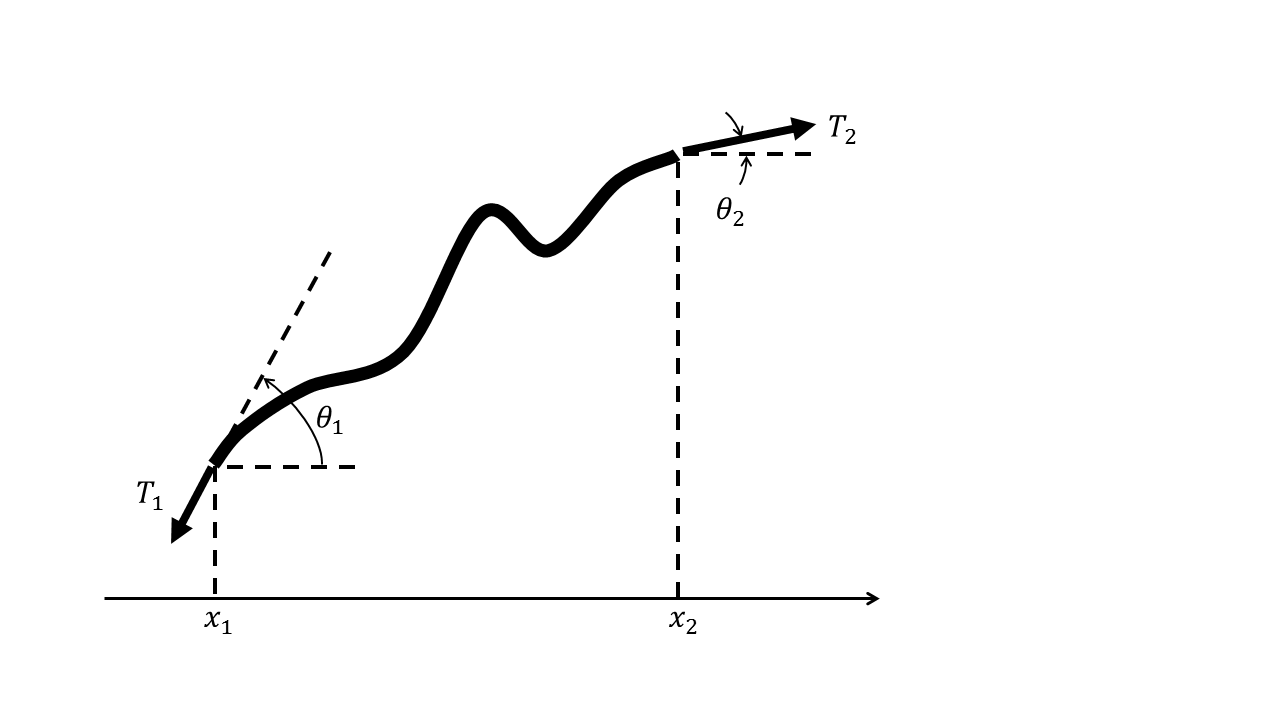
Figure 1: A finite string piece in motion.

Here, we develop a vibrating string model for transverse motions without arguing limits, infinitesimals, or first order approximations. We start with a really finite string piece. Let $T_{1}$ and $T_{2}$ be the tensions, and, $\theta_{1}$ and $\theta_{2}$ be the angles at left and right cuts, respectively (Figure 1). Then, the force balance in $x$ direction dictates

$$T_{1}\cos\theta_{1}=T_{2}\cos\theta_{2}$$ (1)

This relation must hold for any segment, hence for any pair of end points $x_{i}$ and $x_{j}$, at all times. Letting $f(x,t)=T(x,t)\cos(\theta(x,t))$, the fact that $f(x_{i},t)=f(x_{j},t)$ for all $x_{i}$ and $x_{j}$ leads to $f(x,t)=g(t)$. Hence, $T(x,t)=g(t)\sec\theta(x,t)$.

However, tension in the string appears as a reaction to changes in local geometry. Thus, given a shape at any $t^{\ast}$, the tension is dependent on the shape regardless of $t^{\ast}$. As such, explicit dependence of tension on time is not admissible. As a result, we propose

$$T(x,t)=C\sec\theta(x,t)$$ (2)

where $C$ is a constant.

Note that we have not employed any differentials or approximations in obtaining this result. Therefore, simply in order to be compatible with Newton’s second law, regardless of such details as whether bending is included or not, a constitutive model is utilized or not, and so on, and regardless of how complicated or higher order the model is, any string model must conform to this result, provided that only transverse motions are allowed.

Similar things can be done to the transverse motions. The force balance for the finite string piece in transverse direction at any time gives

$$T_{2}\sin\theta_{2}-T_{1}\sin\theta_{1}=y_{tt}(\bar{x})m(x_{1},x_{2})$$ (3)

where $m(x_{1},x_{2})$ is the mass of the segment from $x_{1}$ to $x_{2}$, and $y_{tt}(\bar{x})$ is the acceleration of the center of mass ($\bar{x}$) of the same. Since the mass in $[x_{1},x_{2}]$ is constant, we have

$$m(x_{1},x_{2})=(x_{2}-x_{1})m/L_{0}=(x_{2}-x_{1})\rho$$ (4)

where $\rho$ is the linear density at rest. Therefore,

$$\frac{T_{2}\sin\theta_{2}-T_{1}\sin\theta_{1}}{x_{2}-x_{1}}=\rho y_{tt}(\bar{x})$$ (5)

Letting $x_{1}=x$, $x_{2}=x+h$, $\bar{x}=x_{1}+\alpha\left(x_{1},h,y\right)h$, $\alpha\left(x_{1},h,y\right)>0$, and taking the limit as $h\rightarrow 0$, yields

$$\frac{\partial}{\partial x}(T(x,t)\sin\theta(x,t))=\rho y_{tt}(x,t)$$ (6)

which, with $T(x,t)=C\sec\theta(x,t)$, gives

$$\frac{\partial\theta}{\partial x}\sec^{2}\theta=\frac{\rho}{C}y_{tt}$$ (7)

Now, keeping time fixed and using the fact that $\partial y/\partial x=\tan\theta$, one has

$$\frac{\partial^{2}y}{\partial x^{2}}=\frac{\partial\theta}{\partial x}\frac{\partial\tan\theta}{\partial\theta}=\frac{\partial\theta}{\partial x}\sec^{2}\theta$$ (8)

As a result

$$y_{xx}=\frac{\rho}{C}y_{tt}$$ (9)

This result was obtained by Ciblak (2013) in a more or less similar fashion, Ciblak2013 . Equation 9 is the equation of motion for a vibrating string under the assumption of purely transverse motions, which is exactly what d’Alembert discovered. There are significant differences concerning other things, however. Now,

1. neither the tension nor the length is constant,

2. neither the displacement nor the slopes are assumed to be small,

3. no first order approximations are applied and,

4. both density and area can vary spatially.

Whether or not this departure from the classical model is significant will be demonstrated later.

II.1 Nature of C

Note that the tension can be written as $T(x,t)=Cds/dx$, where $ds$ is the length of a segment over $dx$. Then, one may argue that if at some time $t^{\ast}$ the string has $ds=dx$ everywhere, then the tension would be the same everywhere, say $T_{0}$, i.e. $C=T_{0}$. The existence of a configuration in which $ds(t^{\ast})=dx$ everywhere means $y_{x}(x,t^{\ast})=0$. Then, $y(x,t^{\ast})=0$, due to the boundary conditions. Here, we ignored the discussion of cases in which $ds=dx$ holds in finite intervals of distinct displacements.

Such configurations, $y(x,t^{\ast})=0$, can always be contrived to exist (e.g., for $t^{\ast}<0$). If the spring is considered to be unloaded and at rest prior to the application of initial conditions, then one may safely argue that $y(x,t)=0$ for all $x$, and $t<0$, (simply consider the fact that this is a trivial solution of the string PDE, and thus admissible). This also forces that $y_{x}=0$ in the same domain, giving $T(x,t)=T_{0}$ for all $x$ and $t<0$. As a result, $T_{0}$ is to be interpreted as the internal tension that would result had the spring been unloaded and at rest. Note that this is not equal to the tension in the initial condition.

Also note that if we now claim that the variation of $T(x,t)=T_{0}\sec\theta$ is not negligible, then the same is probably true for the total length

$$L\left(t\right) =\int_{0}^{L_{0}}\sqrt{1+y_{x}^{2}}dx$$

$$L\left(t\right) =\int_{0}^{L_{0}}\sec\theta dx=\frac{1}{T_{0}}\int_{0}^{L_{0}}T\left(x,t\right)dx$$ (10)

II.2 What really happens at $t=0$?

Another counter-intuitive conclusion pertains to the situation at initial condition. For any motion to ensue the string must be given an initial displacement or velocity, or both, which have to be achieved by suitable initial loads. Let’s consider a simple initial displacement as shown in Figure 2 with zero initial velocity.

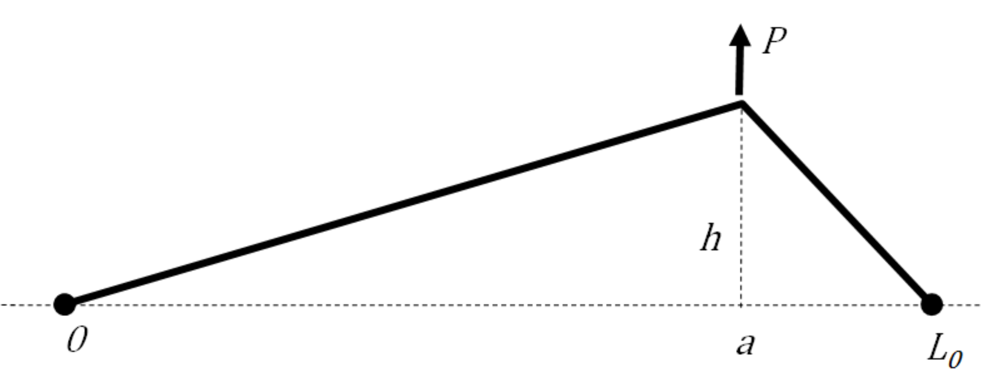
Figure 2: Single kink initial condition with vertical displacement only.

The force $P$ is what is needed to induce the shown displacement. Based on the tension model presented before, the tensions at any point to the left and right of the external force are

$$T_{L} =T_{0}\sec\alpha=T_{0}\sqrt{1+(h/a)^{2}}$$ (11)

$$T_{R} =T_{0}\sec\beta=T_{0}\sqrt{1+(h/\left(L_{0}-a\right))^{2}}$$ (12)

The counter-intuitive point is that these can be quite different, depending on where the force is applied. Why is this so? The answer is simple: it is the result of the requirement that the points move in vertical directions only.

Further, from the force balance in vertical direction at point $a$ one gets

$$P =T_{L}\sin\alpha+T_{R}\sin\beta$$ (13)

$$P =T_{0}(\tan\alpha+\tan\beta)=\frac{T_{0}L_{0}}{a(L_{0}-a)}h$$ (14)

This equation indicates that the string behaves like a linear spring with an equivalent spring stiffness of

$$k_{a}=\frac{T_{0}L_{0}}{a(L_{0}-a)}$$ (15)

Thus, in response to vertical forces, current string model responds like a linear spring, softest at the mid-point ($k_{\min}=4T_{0}/L_{0}$) and stiffening, without bound, as $a$ approaches to the boundaries. This behavior is quite familiar to those who play a plucked string instrument such as guitar.

In any region where the slope vanishes the tension is simply equal to the tension at rest. This could also be the case in the initial condition. This is so even though the tension at neighboring points just outside such portions can differ by a finite amount. For example, if there were two equal forces in the previous figure applied at $a=L_{0}/3$ and $b=2L_{0}/3$ then, as the symmetry would require, the slope within the middle section would have been zero and the tension therein would have to be equal to $T_{0}$.

Again, this behavior is due to the assumption that the string points are allowed to move only in transverse directions. The tension in the mid-section would stay constant because there would be no extension in that section. In reality, however, the tension in the mid-section would increase because some material would leave the region at both ends due to higher tensions in the first and third sections. Thus, in an analysis involving real material behavior the points must be allowed to move in all directions. We shall return to this later.

III UNINTENDED DECEPTION

Up to here, an unsuspecting reader reads with intent and some level of scrutiny, not knowing that he or she was deceived into thinking that everything was fine, equations checked, results made sense, and so on. Yet, the deception is there.

The author of this paper, as a victim of his own writing, also fell for the deception, recovering only recently, after about a year since the original manuscript, Ciblak2013 . That it is an unintended deception does not change the fact that it is a quite powerful one. It is discovered only after the following simple question is posed: what prevents the points of the string from moving horizontally?

From a kinematic point of view, one has the freedom to constrain any point or body to move in certain ways, as long as this does not violate more basic requirements such as continuity. However, this freedom can be bought only in exchange for a constraint force. If a point moves on a circular path, there must be a force that makes it do so. This quite well-known fact was somehow overlooked in both the classical models and the model developed in the previous section, though the latter is intentionally included here only to make a point.

How did these models work, then, if they even did? The classical model escapes this question by invoking the smallness arguments. Whereas, the model developed in previous section does it by tasking the tension to do the balancing. Whether or not this is acceptable we shall show later. For now, the question is how to overcome this obstacle if we still insist on having a transversely vibrating string. We should point out that the material cannot know whether its boundaries or points are constrained or not. Thus, solving the problem by using the material in disguise is meaningless.

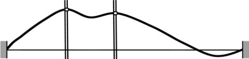
Figure 3: Constraining horizontal motions using vertical rails or slots.

Figure 3 shows a string, two points of which are constrained to move in two vertical slots. We can imagine this to be done for all points of the string. The final result will be a horizontal constraint force distribution that will be responsible for inducing transverse motions. However, this would destroy our basic assumption: the free vibration, or we would have to redefine it.

Such a horizontal force distribution $q(x,t)$ would be given by

$$q(x,t)=-\frac{\partial}{\partial x}(T\cos\theta)$$ (16)

The classical model assumes $\cos\theta\approx 1$ leading to $T=T_{0}$, then yielding $q\left(x,t\right)=0$; whereas the model of the previous section takes $T=T_{0}\sec\theta$, giving $q\left(x,t\right)=-\frac{\partial}{\partial x}(T_{0}\sec\theta\cos\theta)=0$, too. Since the constancy of $T$ is not defendable, we are left with the latter choice, which was developed on the assumption of $q\left(x,t\right)=0$, anyway (the unintended deception).

Thus, our desire to have zero horizontal force distribution determines the tension model for the material, which is only slightly less than magic. Nevertheless, this latter model is really closer to reality, from whence it derives its power, due to the fact that a simple material model reduces to it in a certain limit (see the next section).

III.1 Material model

Instead of the ad hoc material models of previous theories, we now introduce a well-known material model based on Hooke’s law and the linear theory of elasticity. Obviously, one can choose other material models. However, we choose a Hookean model for simplicity and demonstration. Similarly, it is also perfectly allowable to adopt some non-linear theory of elasticity. Considering the cases of finite strain and effects of strain rate, which can actually be quite high, this would have been more prudent. Yet, it would take the focus away from what this study is trying to achieve.

We adopt the definitions of the engineering stress and strain, and the modulus of elasticity, $E$. Let $A_{f}$ be the cross-sectional area of the string when it is non-taut and free, and, $dx_{f}$ be the length of a piece whose length in taut but unloaded case is $dx$. The engineering strain and stress, defined as $\varepsilon=ds/dx_{f}-1$ and $\sigma=T/A_{f}$, respectively, are related as $\sigma=E\varepsilon$. Therefore, one can write

$$T/A_{f} =E(ds/dx_{f}-1)$$ (17)

$$T_{0}/A_{f} =E(dx/dx_{f}-1)$$ (18)

which, after eliminations, gives

$$T=T_{0}\sec\theta+T_{f}(\sec\theta-1)$$ (19)

where $T_{f}=EA_{f}$. Note that $T_{f}$ can be considered as a material constant.

The first term of Equation 19 is the culprit responsible for the deception, with the aid of the second term, of course. For we can now easily see that for very small slopes, the equation reduces to $T=T_{0}$, to that of the classical theory; whereas for small, but not that small slopes, or for $T_{f}=0$, it reduces to that of the model developed here previously, because the second term, $\sec\theta-1$, becomes negligible when compared to the first, $\sec\theta$. The following table summarizes these results.

Slope	Tension Model
General:	$\left(T_{0}+T_{f}\right)\sec\theta-T_{f}$
Small (or $T_{f}=0$):	$T_{0}\sec\theta$
Very Small:	$T_{0}$

Note that the general case is now applicable to strings with zero thickness, too. As to why the linear elastic material model reduces to the classical model may be attributed to the use of lumped masses connected via springs in modeling the string in the latter. However, the reason that it also reduces to the model developed in the previous section remains an open question since we did not invoke any elasticity condition there. This could be taken as a testimony for the ubiquity and success of the Hooke’s law.

The horizontal force distribution needed to induce purely transverse motions can now be given as

$$q(x)=-\frac{T_{f}y_{x}y_{xx}}{\left(1+y_{x}^{2}\right)^{3/2}}=-T_{f}\kappa(x)y_{x}$$ (20)

where $\kappa(x)$ is the curvature. Note that in regions where the string is straight the horizontal load vanishes. This property will be shown to result in important implications.

III.2 True equation of motion for transverse vibrations

Using the new tension relation developed above, the vertical force balance yields the following.

$$\left(1-k\frac{1}{\left(1+y_{x}^{2}\right)^{3/2}}\right)y_{xx} =\frac{1}{c_{f0}^{2}}y_{tt}$$ (21)

$$y_{xx}-k\kappa =\frac{1}{c_{f0}^{2}}y_{tt}$$ (22)

where $k=\frac{T_{f}}{T_{0}+T_{f}}$, $c_{f0}=\sqrt{\frac{T_{0}+T_{f}}{\rho}}$, and $\kappa$ is the curvature. Equation 22 is the correct equation of motion for the transverse vibrations of a string under a horizontal force constraint.

Again, we investigate what happens in certain limits. The results are summarized in the following table.

Slope	Transverse Vibration Model
General:	$\left(1-k\frac{1}{\left(1+y_{x}^{2}\right)^{3/2}}\right)y_{xx}=\frac{1}{c_{f0}^{2}}y_{tt}$
Small:	$(1+\frac{3}{2}\frac{T_{f}}{T_{0}}y_{x}^{2})y_{xx}=\frac{1}{c^{2}}y_{tt}$
Very Small or $k=0$:	$y_{xx}=\frac{1}{c^{2}}y_{tt}$

where $c=\sqrt{\frac{T_{0}}{\rho}}$. Again, the classical model creeps in as a limit case. Note that for $k\rightarrow 0$, either $T_{f}\rightarrow 0$ or $T_{0}\gg T_{f}$.

III.3 Non-taut strings can vibrate, too

In classical treatments, it is as if the case of an initially non-taut string does not exist. Yet, it is a quite familiar reality. What is the equation of motion governing such a string, then? The classical model is completely silent on this question. The model derived above, though still unrealistic, allows one treat initially non-taut, but non-slack, strings. All one has to do is to set $T_{0}=0$, which corresponds to $k=1$. The result is $T=T_{f}(\sec\theta-1)$ and

$$(1-\frac{1}{\left(1+y_{x}^{2}\right)^{3/2}})y_{xx}=\frac{\rho}{T_{f}}y_{tt}=\frac{1}{c_{f}^{2}}y_{tt}$$ (23)

$$y_{xx}-\kappa(x)=\frac{1}{c_{f}^{2}}y_{tt}$$ (24)

where $\kappa(x)$ is the curvature and $c_{f}=\sqrt{\frac{T_{f}}{\rho}}$.

For small slopes, this equation reduces to $y_{tt}=0$, solution of which is $y=v_{0}(x)t+y_{0}(x)$, including the initial conditions. For any fixed boundary conditions, this would yield a non-moving string. For other types, it would yield non-oscillating solutions moving to infinity. Hence, the classical limit of non-taut strings is not meaningful.

However, for the small, but not that small, limit one has:

$$\frac{3}{2}y_{x}^{2}y_{xx} =\frac{1}{c_{f}^{2}}y_{tt}$$ (25)

$$\frac{1}{2}\left(y_{x}^{3}\right)_{x} =\frac{1}{c_{f}^{2}}y_{tt}$$ (26)

Letting $u=y_{x}$, taking the derivatives of both sides with respect to $x$, and using the substitution $\tau=c_{f}t/\sqrt{2}$ gives,

$$(u^{3})_{xx}=u_{\tau\tau}$$ (27)

This is an interesting equation in itself, similar to Burger’s equation.

III.4 Another big oversight

The problems of the classical string models do not end there. Assuming that the proper horizontal force distribution is somewhat maintained during motion so that transverse vibrations are guaranteed, there is still the problem of initial conditions. This discussion can probably be taken as a tribute to what Euler was trying to do.

We shall only concentrate on the initial displacement with zero initial velocity cases. Consider the two distinct initial configurations in Figure 4, which seemingly have identical shapes.

Figure 4: Strings with identical initial shapes, but with distinct displacement fields.

In Figure 4(a), the point of force application is constrained to move along a vertical line, indicated by a linear slot. In this case, the tensions to the left and right of the force are different, in general. Every point to the left of the force experience the same strain thus move vertically without the need for a horizontal force distribution constraint. Same is true for the right section. This can also be found from Equation 20, in which the vanishing second derivatives would result in zero force distributions in each region. The force $Q$ represents the action of the vertical slot. Now, the tensions in left and right regions, $T_{L}$ and $T_{R}$, respectively, are given by

$$T_{L}=(T_{0}+T_{f})\sqrt{1+\left(\frac{h}{a}\right)^{2}}-T_{f}$$ (28)

$$T_{R}=(T_{0}+T_{f})\sqrt{1+\left(\frac{h}{L_{0}-a}\right)^{2}}-T_{f}$$ (29)

The horizontal constraint load is given by

$$Q=T_{f}\left(\frac{1}{\sqrt{1+\left(\frac{h}{a}\right)^{2}}}-\frac{1}{\sqrt{1+\left(\frac{h}{L_{0}-a}\right)^{2}}}\right)$$ (30)

which is curiously independent of the initial tension, and vanishes if $T_{f}=0$. This may be one of the reasons of the apparent success of the classical models.

The vertical force is related to the displacement at $a$ as follows.

$$P =(T_{0}+T_{f})\frac{L_{0}h}{(L_{0}-a)a}$$

$$-T_{f}\left(\frac{h}{\sqrt{(L-a)^{2}+h^{2}}}+\frac{h}{\sqrt{a^{2}+h^{2}}}\right)$$ (31)

Now, the linear dependence of $P$ on $h$ is lost, although it is recovered for sufficiently small $h$ or $T_{f}=0$.

The case in Figure 4(b) is more problematic. The vertical force is applied to a negligibly small and frictionless pulley that allows the tension on both sides to balance. The horizontal force $R$ is responsible for keeping the pulley in a vertical path. In the case shown, i.e. when the point of force application is to the right of the midpoint of the string, the tension would tend to be higher in the right region causing some material to flow from the left to the right, which results in relaxation towards a balance. For example, the material point that was initially at $x=a$ would follow an oblique line into the right region. As a result, despite such a perfectly allowable initial configuration, none of the previous models would be applicable because we now have non-transverse motion or, more correctly, a general motion in $xy$-plane. Note that in this case, when the tension is allowed to balance, the relation $\frac{ds}{d\theta}=\sec\theta$ does not hold any longer.

There are more complicated, yet quite proper, initial configurations that cannot be handled by our simplified models. Figure 5 shows only two of such situations which are quite easily doable, using a simple rubber string, for example. Again, Euler’s assertion, that any initial shape that can be drawn by hand without lifting the pen should be admissible, is true except that he, for some reason, did not consider such simple initial configurations as in Figure 5, which are impossible to handle using d’Alembert’s model.

Obviously, for large displacements one would most likely encounter collisions or self-intersecting shapes. These aside, however, we do not even have a model for small displacements allowing 2D motions or one that can handle simple initial conditions as in Figure 5. All of these point to a need for a more general vibration model for the one dimensional string. One such model is presented in the sequel.

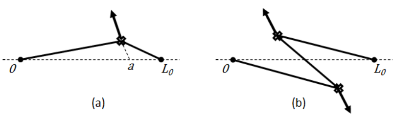
Figure 5: Initial conditions with forced horizontal displacements.

IV 2D VIBRATIONS OF 1D STRING

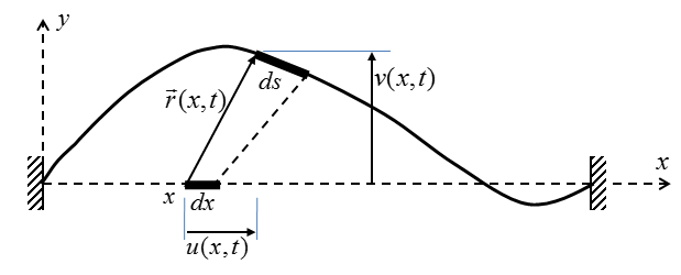
Figure 6: String in 2D motion.

Figure 6 shows a string in general plane motion in which an infinitesimal element originally at $x$, with a length of $dx$, is moved to $(x+u(x,t),v(x,t))$ and stretched to $ds$, where $u(x,t)$ and $v(x,t)$ are the displacement components along the $x$ and $y$ coordinate axes, respectively. The displacement components form scalar fields over the span of $x$ and, for now, we consider them to be at least twice differentiable functions of $x$ and $t$.

The stretched length of the infinitesimal element is given by

$$ds=\sqrt{(1+u_{x})^{2}+v_{x}^{2}}dx$$ (32)

Now, however, $\sec\theta\neq ds/dx$. Nevertheless, the general model for the tension still applies as: $T=(T_{0}+T_{f})ds/dx-T_{f},$ therefore,

$$T=(T_{0}+T_{f})\sqrt{(1+u_{x})^{2}+v_{x}^{2}}-T_{f}$$ (33)

The force balance equations remain simple:

$$u_{tt}dm =d(T\cos\theta)$$ (34)

$$v_{tt}dm =d(T\sin\theta)$$ (35)

Now, we use the following.

$$\cos\theta =\frac{1+u_{x}}{\sqrt{(1+u_{x})^{2}+v_{x}^{2}}}$$ (36a)

$$\sin\theta =\frac{v_{x}}{\sqrt{(1+u_{x})^{2}+v_{x}^{2}}}$$ (36b)

and $$dm=\rho_{0}dx \rho_{0}$$, where is the linear density at rest, to get the final result presented below.

$$\frac{1}{c_{f0}^{2}}u_{tt} =u_{xx}-k\frac{\partial}{\partial x}\frac{1+u_{x}}{\sqrt{(1+u_{x})^{2}+v_{x}^{2}}}$$ (37)

$$\frac{1}{c_{f0}^{2}}v_{tt} =v_{xx}-k\frac{\partial}{\partial x}\frac{v_{x}}{\sqrt{(1+u_{x})^{2}+v_{x}^{2}}}$$ (38)

where $k=\frac{T_{f}}{T_{0}+T_{f}}$ and $c_{f0}=\sqrt{\frac{T_{0}+T_{f}}{\rho_{0}}}$.

Equations 37 and 38 are the equations of motion for the one-dimensional string in $xy$-plane and are the main results of this study.

As a justification, we present below some limit cases, in which $k=0$ cases correspond to $T_{f}=0$ or $T_{0}>>T_{f}$, whereas $k=1$ cases correspond to $T_{0}=0$ or $T_{0}<<T_{f}$. The definitions $c^{2}=T_{0}/\rho_{0}$, $c_{f}^{2}=T_{f}/\rho_{0}$, $c_{f0}^{2}=\left(T_{f}+T_{0}\right)/\rho_{0}$ are used throughout. Also note that, for a string with a vanishing thickness one has $T_{f}=0$, leading to $k=0$.

IV.1 CASE: Transverse motion only

In this mode $u=0$ and Equation 37 can be satisfied only if $k=0$ (since $v_{x}\neq 0$, for motion). Therefore, for transverse motions one must have $T_{f}=0$. This is true only for a vanishingly thin string $(A_{f}=0)$ or a material with no resistance to stretching $(E=0)$. The case of very taut string $(T_{0}>>T_{f})$ also approximates this mode. With $T_{f}=0$ the tension, the horizontal constraint force, and the remaining equation of motion become

$$T =T_{0}\sqrt{1+v_{x}^{2}}=T_{0}\sec\theta$$ (39)

$$q(x,t) =-\frac{\partial}{\partial x}(T\frac{1}{\sqrt{1+v_{x}^{2}}})=0$$ (40)

$$\frac{1}{c_{f0}^{2}}v_{tt} =\frac{1}{c^{2}}v_{tt}=v_{xx}$$ (41)

This is where lies the reason of the apparent success of the classical string theory, as it is modified by Ciblak, Ciblak2013 . This time, however, the tension model based on a simple linear elastic behavior seems to be exactly what is needed to rescue the classical string model. Nevertheless, in following sections we show that pure transverse motions are possible only in rare cases.

Note that pure transverse motions are possible using kinematic constrains such as a discrete vertical rail systems. However, these introduce hidden boundary conditions which are not declared anywhere, as well as making the problem look like an unnatural contraption without any justification. In such cases, the horizontal constraint force vanishes in between the rails. Therefore, kinematic constraints such as discrete rails require discrete, horizontal point forces.

In the rest of this study we only explore the admissibility of pure transverse motions without any kinematic constraints. In other words, we look for cases in which $q\left(x,0\right)$ is whatever needed to induce pure transverse displacements at $t=0$, yet $q\left(x,t\right)=0$ ($t>0$) despite having truly pure transverse motions without any kinematic constraints.

IV.2 CASE: Horizontal motion only

The conditions necessary to induce this mode are: $v=0$ and $\theta=0$, leading to $ds/dx=1+u_{x},$ and $w(x)=0$ (vertical constraint force). The equations of motion become

Limit	Equations
General:	$u_{tt}=c_{f0}^{2}u_{xx}$
$k=0$: (A material model)	$u_{tt}=c^{2}u_{xx}$
$k=1$: (Non-taut string)	$u_{tt}=c_{f}^{2}u_{xx}$

with the following tension models.

Limit	Tension
General:	$T=T_{0}\left(1+u_{x}\right)+T_{f}u_{x}$
$k=0$: (A material model)	$T=T_{0}\left(1+u_{x}\right)$
$k=1$: (Non-taut string)	$T=T_{f}u_{x}$

Interestingly, the pure horizontal motion case does not suffer from any troubles similar to what engulfed the pure transverse motions. This is because the pure horizontal motion, including the initial conditions, does not affect the vertical displacement.

IV.3 CASE: $k=0$ (a material model)

In this case the tension becomes $T=T_{0}\sqrt{(1+u_{x})^{2}+v_{x}^{2}}$, and the equations reduce to

$$u_{tt}=c^{2}u_{xx}$$

(42)

IV.4 CASE: $k=1$ (initially non-taut/non-slack string)

Now, $T=T_{f}\left(\sqrt{(1+u_{x})^{2}+v_{x}^{2}}-1\right)$ and the equations reduce to

$$\frac{1}{c_{f}^{2}}u_{tt}=u_{xx}-\frac{\partial}{\partial x}\frac{1+u_{x}}{\sqrt{(1+u_{x})^{2}+v_{x}^{2}}}$$

(43)

It can be seen that the classical model and the non-taut model are the two distinct limits of the general 2D motions of the 1D string.

IV.5 Vector form and extension to higher dimensions

Using a substitution $\mathbf{r}=[1+u_{x},v_{x}]^{T}\in R^{2}-\{\mathbf{0}\}$, a vector form of 2D vibrations,

$$\frac{1}{c_{f0}^{2}}\mathbf{r}_{tt}=\mathbf{r}_{xx}-k\frac{\partial^{2}}{\partial x^{2}}\left(\frac{\mathbf{r}}{\left\|\mathbf{r}\right\|}\right)$$ (44)

is obtained, which can be used as a basis for extending the result to $n$ dimensional motions of a 1D string. That is, by letting $\mathbf{r}=[1+u_{x},v_{1x},v_{2x},...,v_{(n-1)x}]^{T}\in R^{n}-\{\mathbf{0}\}$, Equation 44 can be interpreted as describing the motion of a 1D string in $n$ dimensional space, where $v_{ix}$ are the displacement gradients in directions perpendicular to $x$.

V INITIAL CONDITIONS FOR 2D MOTIONS

We now return to the question of initial conditions, which is not a straightforward problem as was seen in previous sections. In general, the initial spatial configuration must satisfy the following.

$$q(x) =-(T_{0}+T_{f})\frac{\partial}{\partial x}\left(U_{0x}-k\frac{U_{0x}}{\sqrt{U_{0x}^{2}+v_{0x}^{2}}}\right)$$ (45a)

$$w(x) =-(T_{0}+T_{f})\frac{\partial}{\partial x}\left(v_{0x}-k\frac{v_{0x}}{\sqrt{U_{0x}^{2}+v_{0x}^{2}}}\right)$$ (45b)

where $$U_{0x}=1+u_{0x} u_{0x} v_{0x} t=0 q w Q(x)=\int q(x)dx W(x)=\int w(x)dx$$ and, and are displacement gradients at , and, and are the horizontal and vertical force distributions, respectively. If the force distributions are given, equations 45 can be used to determine the initial displacement gradients. For example, let and . Then, the solutions are

$$u_{0} =\int\left(1+\frac{k}{\sqrt{A_{1}^{2}+A_{2}^{2}}}\right)A_{1}dx+c_{3}-x$$ (46)

$$v_{0} =\int\left(1+\frac{k}{\sqrt{A_{1}^{2}+A_{2}^{2}}}\right)A_{2}dx+c_{4}$$ (47)

$$\left(\frac{ds}{dx}\right)_{0} =k+\sqrt{A_{1}^{2}+A_{2}^{2}}$$ (48)

$$T =(T_{0}+T_{f})\sqrt{A_{1}^{2}+A_{2}^{2}}$$ (49)

where $A_{1}=c_{1}-\frac{Q(x)}{T_{0}+T_{f}}$ and $A_{2}=c_{2}-\frac{W(x)}{T_{0}+T_{f}}$, and $c_{i}$ are arbitrary constants, which should be determined from the boundary conditions on $u_{0}$ and $v_{0}$. A useful special case is summarized in the following proposition.

Proposition 1

A segment of the string in the initial condition is free of external forces if and only if the displacement gradients (or, equivalently, the extension ratio or the tension) are constant therein.

Proof. If a segment if free of external forces then equations 45 yield, after an integration, two algebraic equations of the gradients, whose solution can be shown to uniquely exist. If the gradients are constant in a segment then the same equations give zero external force distributions. Note that in such a segment both the tension and the extension ratio remain constant by virtue of their definitions.   

If, instead of the external forces, the initial shape is given, then the situation is more involved. Now, equations 45 can only be used to determine the required force distributions. Thus, we have to find other ways of determining the initial displacement fields.

However, as discussed earlier, the initial shape alone is not enough to determine the initial situation. There could be infinitely many initial configurations that yield the same shape. Further, in contradiction to what Euler stated, there are initial shapes that can be drawn by hand without lifting the pen, but cannot be represented by a simple function. An example of this was given in Figure 5(b). This issue will be addressed later.

Assuming now that the initial shape can be given as $y_{0}(x)$, we distinguish two major categories: a) those in which the string is allowed to initially equalize the internal tension, b) and those in which it is not. The latter requires the description of each particular case as well as introducing extra boundary conditions. Therefore, we concentrate on the former by stating the following theorem.

Theorem 2

Let the initial shape of the string be given by a continuous and piecewise differentiable function $y_{0}(x)$ that satisfies the boundary conditions. If the tension is the same everywhere initially, then the initial displacement fields are given by

$$u_{0}(x) =L^{-1}\left(\frac{L(L_{0})}{L_{0}}x\right)-x$$ (50)

$$v_{0}(x) =y_{0}\left(x+u_{0}\right)$$ (51)

where $L\left(z\right)=\int_{0}^{z}\sqrt{1+\left(y_{0}^{\prime}\left(\zeta\right)\right)^{2}}d\zeta$ is the length function defined over $[0,L_{0}]$. Further, $u_{0}(x)$ and $v_{0}(x)$ automatically satisfy the boundary conditions.

Proof. Based on the properties of $y_{0}(x)$ and the form of the integrand, the length function

$$L(z)={\displaystyle\int\limits_{0}^{z}}\sqrt{1+\left(y_{0}^{\prime}\left(\zeta\right)\right)^{2}}d\zeta\text{ \ \ \ \ \ }z\in[0,L_{0}]$$ (52)

is continuous and strictly increasing. Therefore, the inverse function $L^{-1}(z)$ exists. Since the tension is constant throughout, then so is

$$\left(\frac{ds}{dx}\right)_{0}=\frac{L(L_{0})}{L_{0}}$$ (53)

where $L(L_{0})$ is the initial length. From the first of equations 36 one gets

$$\sqrt{1+\left(y_{0}^{\prime}\left(x+u_{0}\right)\right)^{2}}d\left(x+u_{0}\right)=\left(\frac{ds}{dx}\right)_{0}dx$$ (54)

Now, by integrating both sides, we have

$$L(x+u_{0})=\frac{L(L_{0})}{L_{0}}x$$ (55)

with the boundary condition at $x=0$ applied. Then

$$u_{0}\left(x\right)=L^{-1}\left(\frac{L(L_{0})}{L_{0}}x\right)-x$$ (56)

where $L^{-1}(z)$ is the inverse function for $L(z)$.

One can see from Figure 6 that a point originally at $x$ is moved horizontally to $x+u_{0}$ and then lifted vertically by an amount of $v_{0}$, ending up at $y_{0}\left(x+u_{0}\right)$. Therefore, it follows that $v_{0}\left(x\right)=y_{0}\left(x+u_{0}\right)$.

The boundary conditions on $u_{0}$ are automatically satisfied: $u_{0}(0)=L^{-1}\left(0\right)-0=0$ and

$$u_{0}(L_{0}) =L^{-1}\left(\frac{L(L_{0})}{L_{0}}L_{0}\right)-L_{0}$$ (57)

$$=L^{-1}\left(L(L_{0})\right)-L_{0}=0$$ (58)

Also, $v_{0}=y_{0}\left(x+u_{0}\right)$ yields

$$v_{0}(0) =y_{0}\left(0+u_{0}(0)\right)=y_{0}\left(0\right)=0$$

$$v_{0}(L_{0}) =y_{0}\left(L_{0}+u_{0}(L_{0})\right)=y_{0}\left(L_{0}\right)=0$$

 

V.1 Analytical verification of Theorem 2

Before proceeding to numerical studies, a verification of the above theorem can be presented. Consider the singly kinked initial condition as depicted in Figure 4(b), where tension equalization is assumed. Clearly,

$$\left(\frac{ds}{dx}\right)_{0}=\frac{\sqrt{a^{2}+h^{2}}+\sqrt{\left(L_{0}-a\right)^{2}+h^{2}}}{L_{0}}$$ (59)

We first derive the forms of the initial displacements using the geometry only. For this, it is sufficient to determine which point $(x_{1},0)$ is mapped to $(a,h)$. From the figure is it seen that $x_{1}$ must be such that

$$\frac{\sqrt{a^{2}+h^{2}}}{x_{1}}=\left(\frac{ds}{dx}\right)_{0}=\frac{L(L_{0})}{L_{0}}$$ (60)

$$x_{1}=\frac{\sqrt{a^{2}+h^{2}}}{\sqrt{a^{2}+h^{2}}+\sqrt{\left(L_{0}-a\right)^{2}+h^{2}}}L_{0}$$ (61)

Now, by Proposition 1, $u_{0}$ and $v_{0}$ are linear functions in force-free segments. Hence,

$$u_{0}\left(x\right)=\left\{\begin{array}[c]{ccc}\frac{a-x_{1}}{x_{1}}x&&0\leq x\leq x_{1}\\ \frac{a-x_{1}}{L_{0}-x_{1}}\left(L_{0}-x\right)&&x_{1}\leq x\leq L_{0}\end{array}\right.$$ (62)

$$v_{0}\left(x\right)=\left\{\begin{array}[c]{ccc}\frac{h}{x_{1}}x&&0\leq x\leq x_{1}\\ \frac{h}{L_{0}-x_{1}}\left(L_{0}-x\right)&&x_{1}\leq x\leq L_{0}\end{array}\right.$$ (63)

Next, we show this result using Theorem 2. The initial shape and the length function are given by

$$y_{0}\left(x\right)=\left\{\begin{array}[c]{ccc}\frac{h}{a}x&&x\leq a\\ \frac{h}{L_{0}-a}\left(L_{0}-x\right)&&x\geq a\end{array}\right.$$ (64)

$$L\left(z\right)=\left\{\begin{array}[c]{ccc}s_{1}z&&z\leq a\\ s_{2}z-\left(s_{2}-s_{1}\right)a&&z\geq a\end{array}\right.$$ (65)

where $z\in\left[0,L_{0}\right]$, $s_{1}=\sqrt{1+\left(\frac{h}{a}\right)^{2}}$, and $s_{2}=\sqrt{1+\left(\frac{h}{L_{0}-a}\right)^{2}}$. The inverse of the length function is

$$L^{-1}\left(z\right)=\left\{\begin{array}[c]{ccc}\frac{z}{s_{1}}&&z\leq s_{1}a\\ \frac{z+\left(s_{2}-s_{1}\right)a}{s_{2}}&&z\geq s_{1}a\end{array}\right.$$ (66)

where $z\in\left[0,L(L_{0})\right]$. Let

$$L(L_{0})=\sqrt{a^{2}+h^{2}}+\sqrt{\left(L_{0}-a\right)^{2}+h^{2}}=L_{i}$$ (67)

Then, by Theorem 2,

$$u_{0}=L^{-1}\left(\frac{L_{i}}{L_{0}}x\right)-x$$ (68)

$$u_{0}=\left\{\begin{array}[c]{ccc}\frac{L_{i}/L_{0}}{s_{1}}x-x&&x\leq\frac{L_{0}}{L_{i}}s_{1}a\\ \frac{L_{i}/L_{0}x-s_{1}a}{s_{2}}+a-x&&x\geq\frac{L_{0}}{L_{i}}s_{1}a\end{array}\right.$$ (69)

Note that $\frac{L_{0}}{L_{i}}s_{1}a$ is equal to $x_{1}$. After manipulations, one gets Equation 62 exactly. The switching point for $y$, $x=a$, corresponds to that of $x+u_{0}$, which corresponds to that of $u_{0}$, $x=x_{1}$. Therefore, we simply insert the piecewise definitions in their corresponding places in $y(x+u_{0})$ to get

$$v_{0}=$$ (70)

$$\left\{\begin{array}[c]{ccc}\frac{h}{a}\left(\frac{a-x_{1}}{x_{1}}x+x\right)&&x\leq x_{1}\\ \frac{h}{L_{0}-a}\left(L_{0}-\left(\frac{a-x_{1}}{L_{0}-x_{1}}\left(L_{0}-x\right)+x\right)\right)&&x\geq x_{1}\end{array}\right.$$ (73)

which, after simplifications, reduces to Equation 63. This verifies the theorem.

For other types of initial shape functions, obtaining the explicit form of $u_{0}$ involving simple functions becomes almost impossible or quite complicated. For example, for an initial sine or cosine shape, $L(z)$ involves elliptic integrals. Nevertheless, numerical implementation is quite straightforward, which is used in every example of the next section on numerical experiments. This clearly demonstrates the usefulness of Theorem 2.

V.2 Initial conditions that are compatible with purely transverse motions

If $u_{0}\neq 0$ at $t=0$, then horizontal motions for $t>0$ are unavoidable because the related equation of motion becomes $u_{tt}=c^{2}u_{xx}$, for which $u\left(x,t\right)=0$ is not a viable solution since it does not satisfy the initial conditions. Therefore, in addition to $k=0$, another necessary condition for purely transverse motions is $u_{0}\left(x\right)=0$. This forces, by Theorem 2, that

$$L\left(x\right)=\frac{L(L_{0})}{L_{0}}x$$ (74)

This can happen only if the $y_{0}^{\prime}\left(x\right)$ is constant in at most a piecewise manner. If $y_{0}^{\prime}\left(x\right)=0$ over the whole domain then by the virtue of the boundary conditions $y_{0}\left(x\right)=0$, which we discard since it results in no motion. Hence, $y_{0}^{\prime}\left(x\right)$ can be constant only in a piecewise manner over finite regions, the union of which would equal $\left[0,L_{0}\right]$. Therefore, a consequence of $u_{0}\left(x\right)=0$ is that the initial shape $y_{0}\left(x\right)$ can only have straight segments in a piecewise continuous manner, simplest case of which is Euler’s singly kinked initial condition. This explains the apparent success of Euler’s proposal.

Note that an initial shape with straight segments in a piecewise manner restricts the initial horizontal forces to be only point forces, a result which we obtained previously after a different line of reasoning.

The initial shape can be obtained in two ways: a) by allowing tension equalization, i.e. with zero horizontal constraint force, b) by using initial horizontal point forces at kinks. In the latter case, as soon as the string is released the horizontal constraint forces disappear. The discontinuity in the initial tension around kinks caused by the horizontal forces now creates an imbalance due to the absence of them just after the release. This will cause horizontal motions. Therefore, for purely transverse motions it is also necessary that the tension be allowed to balance, which amounts to zero horizontal force constraints.

If the initial tension is uniform over the whole string then the slopes of the straight segments on either side a kink must be equal in magnitude and opposite in sign in order to preserve force balance in horizontal direction when the motion starts. It is simple to show that this must be true for all kinks. That is, the magnitudes of the slopes of all segments must be the same. Hence, we proved the following.

Theorem 3

The necessary and sufficient conditions for a string to execute purely transverse motions are:

1. $k=\frac{T_{f}}{T_{0}+T_{f}}=0$, i.e. either $E=0$, $A_{f}=0,$ or $T_{0}\gg T_{f}$.

2. Initial shape must be formed by straight segments around discretely distributed kink points,

3. There are no initial horizontal force constraints, or, equivalently, the initial tension is uniform everywhere,

4. Magnitudes of slopes of all segments must be the same and signs of those on each side of a kink point must be opposite.

It is now seen clearly that pure transverse vibrations of an ideal string are indeed rarities. For a single kink case, the string must be lifted at the mid-span. Therefore, Euler’s proposal is acceptable only when the kink point is at the middle. Otherwise, pure transverse motions are not possible.

For multiple kinks, the situation becomes interesting. If we start with a positive slope at $x=0$, without loss of generality, and if each segment is represented by a vector $\bar{r}_{i}$, $i=1,\cdots,N$, where $N$ is the number of segments, then we can write down the following vector loop equation.

$$\sum_{i=1}^{N}\bar{r}_{i}=\sum_{i=1}^{N}r_{i}\left[\begin{array}[c]{c}\cos\alpha\\ \left(-1\right)^{i+1}\sin\alpha\end{array}\right]=\left[\begin{array}[c]{c}L_{0}\\ 0\end{array}\right]$$ (75)

where $r_{i}$ is the length of $i^{\text{th}}$ segment and $\alpha$ is the magnitude of the slope angle for all segments. By letting $L_{i}=r_{i}\cos\alpha$, projected length on $x$-axis, one gets

$$\sum_{i=1}^{N}\left[\begin{array}[c]{cc}L_{i}&\left(-1\right)^{i+1}L_{i}\tan\alpha\end{array}\right]^{T}=\left[\begin{array}[c]{cc}L_{0}&0\end{array}\right]^{T}$$ (76)

which leads to the following scalar equations.

$$\sum_{i=1}^{N}L_{i} =L_{0}$$ (77)

$$\sum_{i=1}^{N}\left(-1\right)^{i+1}L_{i} =0$$ (78)

regardless of $\alpha$. Note that the special cases $\alpha=\pm\frac{\pi}{2}$ are not viable. These equations have a unique solution only when $N=2$, namely

$$L_{1}=L_{2}=\frac{L_{0}}{2}$$

which correspond to the example of a string lifted at the middle point, as was discussed earlier.

Equations 77 and 78 lead to

$$\sum_{i=1\text{ odds}}^{N}L_{i}=\sum_{i=2\text{ evens}}^{N}L_{i}=\frac{L_{0}}{2}$$ (79)

For $N>2$ one would have a family of solutions that depend on $N-2$ parameters. Let $L_{1}$ and $L_{2}$ be the dependent variables and $L_{i}$, $i>2$, be taken as free parameters. Then, the solutions for $L_{1}$ and $L_{2}$ in terms of the free parameters are

$$L_{1} =\frac{L_{0}}{2}-\sum_{i=3}^{N}L_{i}\text{ \ \ (}i\text{ is odd)}$$

$$L_{2} =\frac{L_{0}}{2}-\sum_{i=4}^{N}L_{i}\text{ \ \ (}i\text{ is even)}$$

provided that $L_{i}\geqslant 0$ for all $i$.

Note that for any given number of segments, $N$, one gets all others, $n=2,3,\cdots,N-1$ by setting the lengths of $N-n$ segments to zero.

As a demonstration we consider $N=3$, for which we have the following result.

$$L_{1} =\frac{L_{0}}{2}-L_{3}$$

$$L_{2} =\frac{L_{0}}{2}$$

where $L_{3}\in\left[0,\frac{L_{0}}{2}\right]$ is the free parameter. Figure 7 shows three examples of initial shapes with two kinks. For all cases the slope angle is $\pm 45{{}^{\circ}}$. The solid line is when $L_{3}=\frac{1}{4}$ and the dashed line below corresponds to $L_{3}=0.4$. The dotted-dashed line above is for $L_{3}=0$. It is seen that the single kink solution is a limit case of two-kink solutions, as discussed earlier. It is easily seen how all other solutions can be obtained geometrically. Also note that the points where the shape intersects the $x-$axis are vibration nodes. Figure 8 illustrates initial shapes with three kinks.

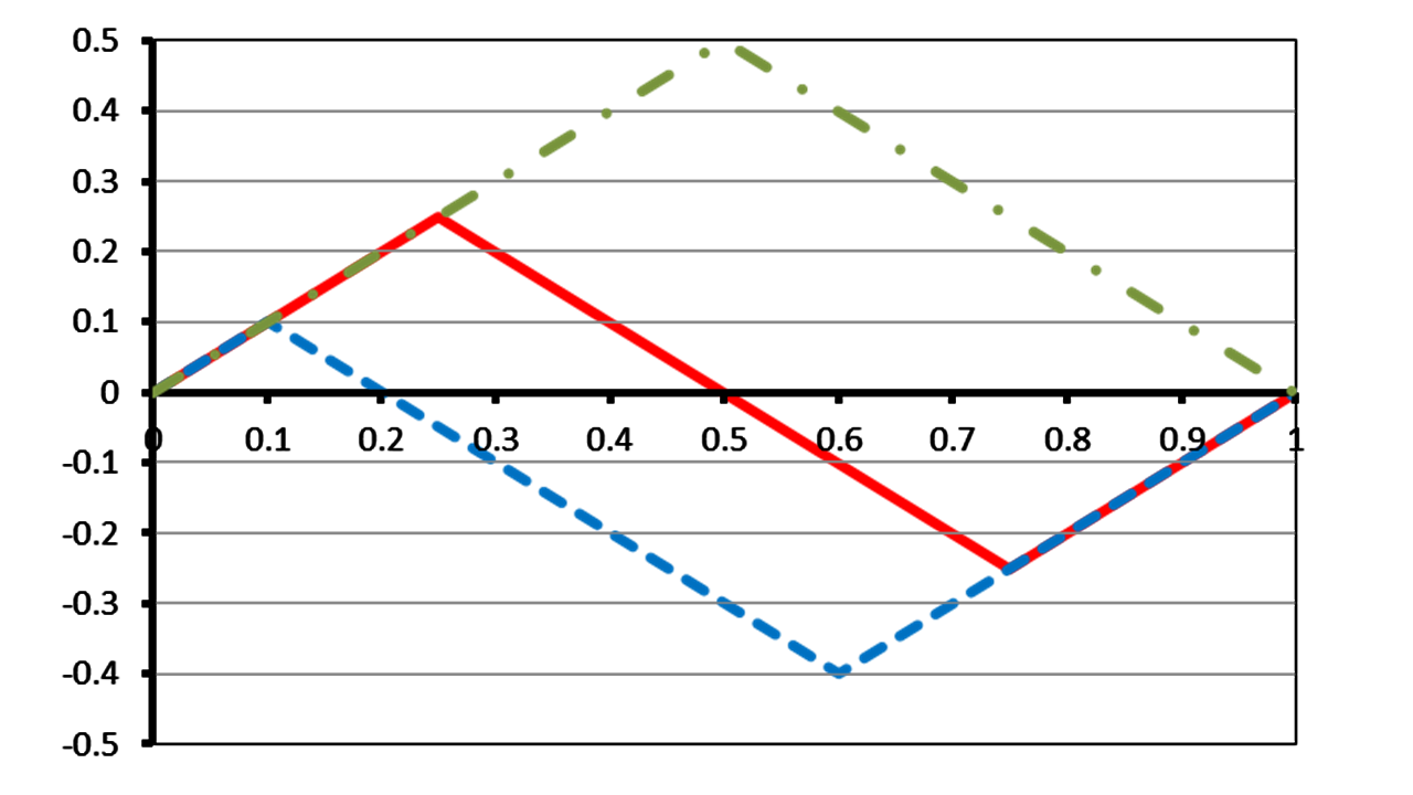
Figure 7: Initial shapes with two kinks and with equal and opposite slopes on each side of kinks. All slope angles are $\pm 45{{}^{\circ}}$.

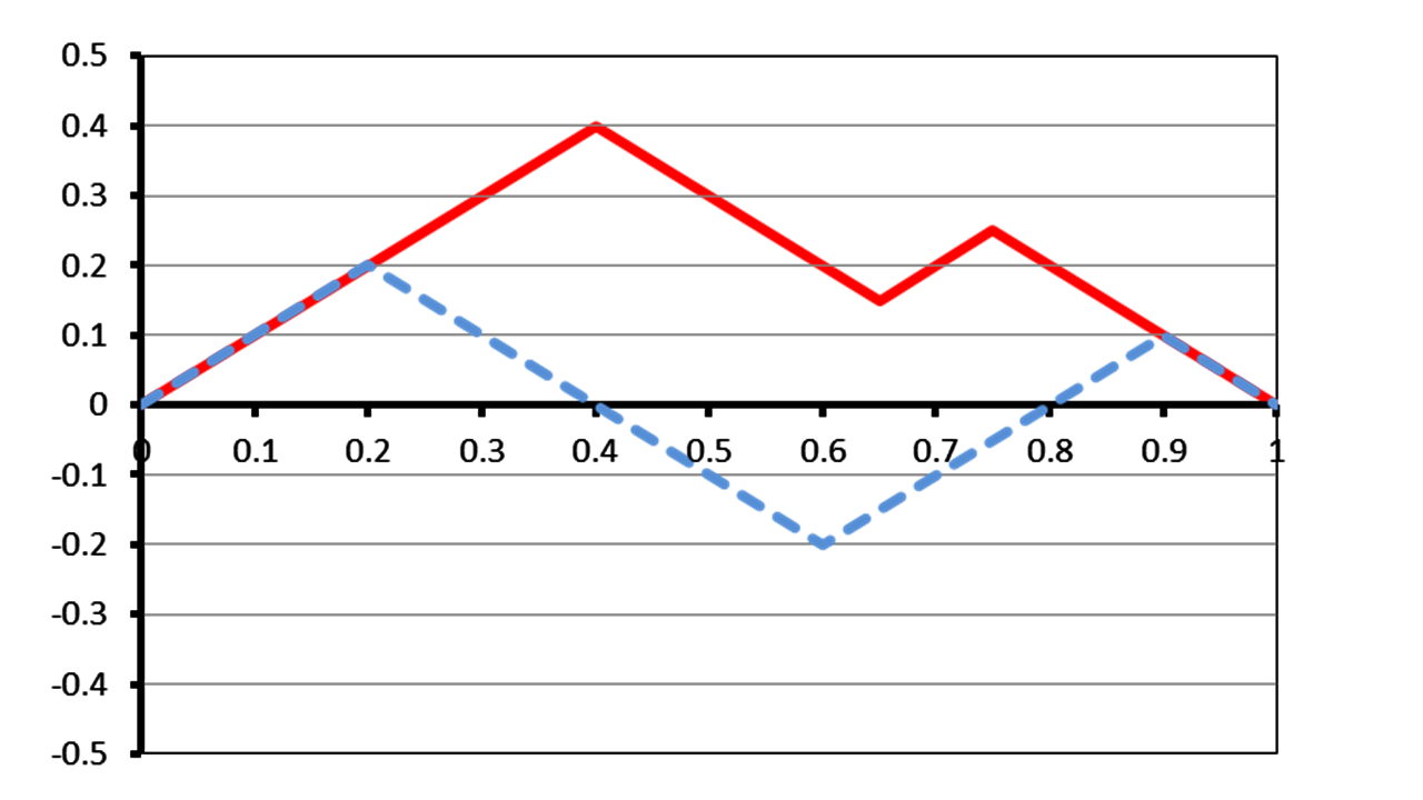
Figure 8: Initial shapes with three kinks and with equal and opposite slopes on each side of kinks. All slope angles are $\pm 45{{}^{\circ}}$.

Another interesting, yet expected, result pertains to the form of the length function. Since the slopes of the segments are constant up to a sign difference the integrand in the definition of the length function becomes

$$\sqrt{1+\left(y_{0}^{\prime}\left(x\right)\right)^{2}}=\sqrt{1+\tan^{2}\alpha}=\sec\alpha$$ (80)

regardless of the segment. Therefore, despite having a piecewise defined shape, the length function is simply given by

$$L\left(z\right)=\left(\sec\alpha\right)z$$ (81)

for all $z\in\left[0,L_{0}\right]$, the inverse of which is

$$L^{-1}\left(z\right)=\frac{1}{\sec\alpha}z=\left(\cos\alpha\right)z$$ (82)

This result can be used to prove the following.

Proposition 4

Provided that the initial tension is equalized, the initial horizontal displacement is zero, $u_{0}\left(x\right)=0$, if and only if the initial shape is formed by straight segments between isolated kinks, on each side of which the segment slopes are equal and opposite.

Proof. That $u_{0}=0$ implies the initial shape is as declared in the proposition was proven in Theorem 3. For the converse, one assumes that the initial shape is as declared. Then, by Theorem 2 (since the tension is uniform), and, equations 81 and 82, one would have

$$u_{0} =L^{-1}\left(\frac{L(L_{0})}{L_{0}}x\right)-x$$ (83)

$$=L^{-1}\left(\frac{\left(\sec\alpha\right)L_{0}}{L_{0}}x\right)-x$$ (84)

$$=L^{-1}\left(\left(\sec\alpha\right)x\right)-x$$ (85)

$$=\left(\cos\alpha\right)\left(\sec\alpha\right)x-x=0$$ (86)

which completes the proof of the proposition.   

This proposition now leads to the following theorem, the proof of which is straightforward and, therefore, omitted.

Theorem 5

Given that $k=0$ and the initial tension is equalized, an ideal string executes purely transverse motions if and only if the initial shape is formed by straight segments between isolated kinks, on each side of which the segment slopes are equal and opposite.

In the sequel, the effect of initial conditions is explicitly demonstrated by numerical experiments. Further, we also present, from the results of actual experiments, the fact that a string with conditions close to the ideal cannot help but execute horizontal motions.

VI NUMERICAL EXPERIMENTS

In this section, we present numerical analyses of various interesting cases in order to demonstrate the findings of previous sections. Both the process of setting up of initial conditions and resulting solutions are discussed. For verification, the solutions are obtained, whenever possible, on two different numerical analysis platforms using different methods.

VI.1 Two distinct cases with the same linear shape

In Figure 4(a), the tensions are different in the left and the right regions. By Proposition 1, the extension ratio in the left region is $\sqrt{1+\left(h/a\right)^{2}}$. Since points $x=0$ and $x=a$ are mapped to themselves, again by Proposition 1, $u_{0}(x)=0$, which, after applying the left boundary condition, gives $v_{0,x}=h/a$, or $v_{0}=(h/a)x$. Similar results are obtained for the right region. Thus, we have $u_{0}=0$ and

$$v_{0}=\left\{\begin{array}[c]{cc}\frac{h}{a}x&0\leqslant x\leqslant a\\ \frac{h}{L_{0}-a}\left(L_{0}-x\right)&a\leqslant x\leqslant L_{0}\end{array}\right.$$ (87)

The case of Figure 4(b), in which the tension is equalized, was studied earlier and the displacement fields were given in equations 62 and 63.

The two problems in Figure 4 are quite different from each other, although they are governed by the same equations of motion and the initial shape of the string looks the same. In Figure 4(a), the points initially move vertically up. However, as soon as the motion starts the points will also execute horizontal motions due to the imbalance between the tensions, unless $a=L_{0}/2$. Whereas, in Figure 4(b) the points will certainly undergo horizontal motions, because they are already displaced horizontally in the initial configuration.

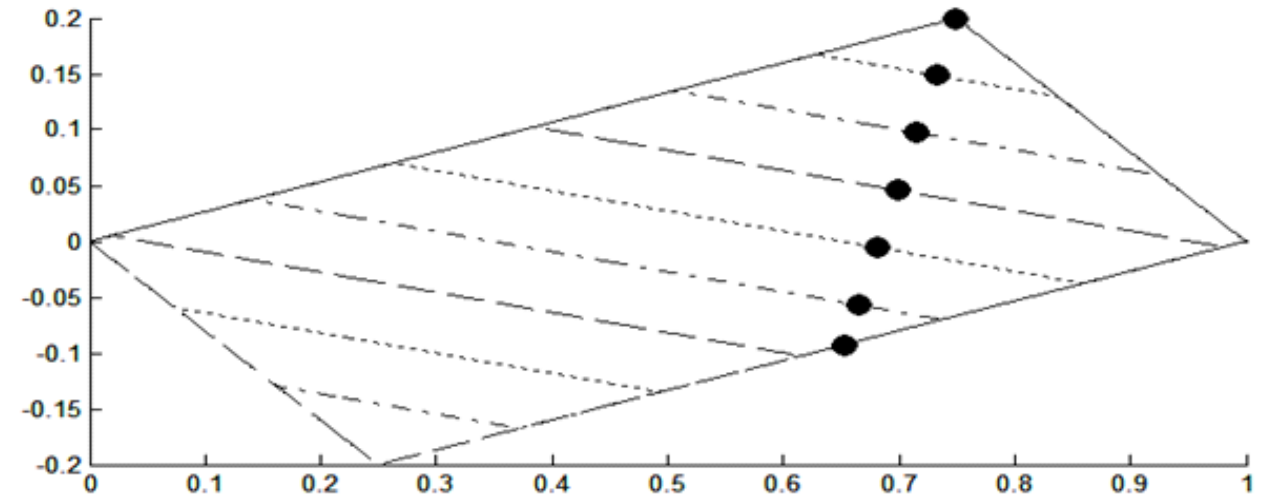
Figure 9: String with an initial single kink in motion. The dark dot is the path of the kink point. Case: $k=0$.

Figure 9 shows the motion for case (b) and the trace of the kink point. All points, except the boundaries, move such that they dwell for a finite duration when they reach the outer envelopes. Then, they move in the opposite direction starting with infinite accelerations, a behavior that can be easily observed using Euler’s solutions. This is an unavoidable consequence of the chosen material model.

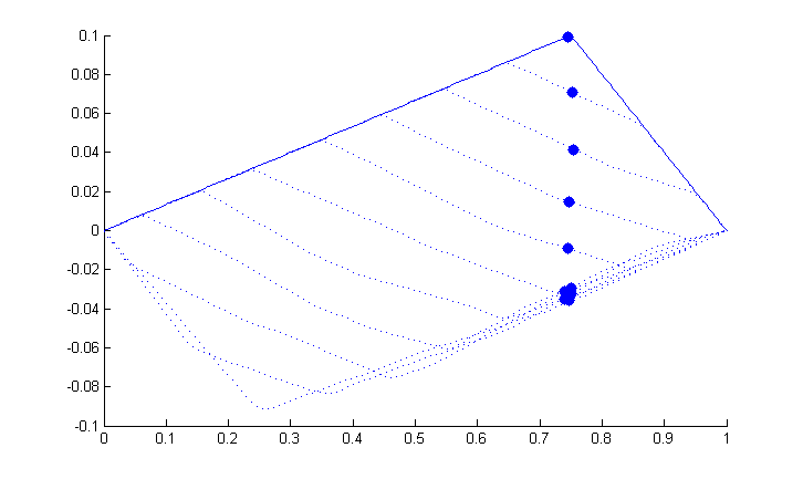
Figure 10: A singly kinked string solution. The kink point was initially constrained to move vertically only. Case: $k>0$.

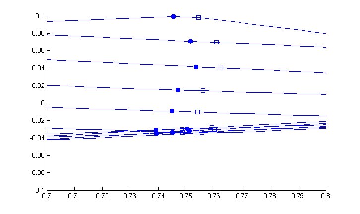
Figure 11: Detail around the single kink (initially constrained). The points first move towards right due to higher tension, then towards left due to horizontal oscillation.

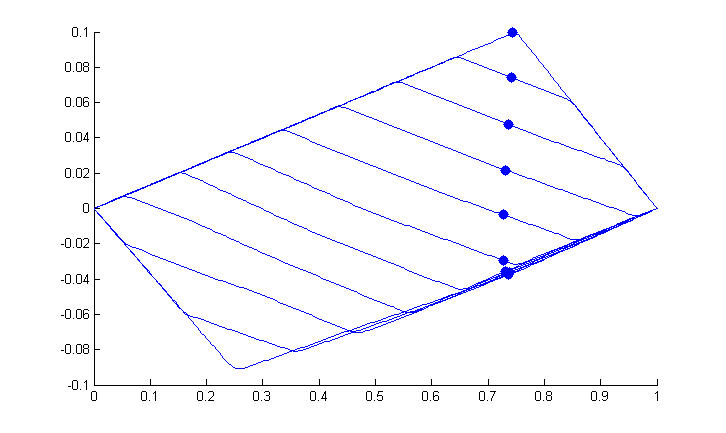
Figure 12: A singly kinked string solution. The tension is equalized initially. The final kink point originates from a point in the left region. Case: $k>0$.

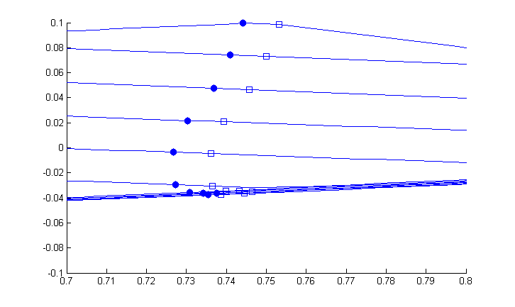
Figure 13: Detail around the single kink (initially relaxed). The points first move towards left due to initial horizontal force field, then towards right due to horizontal oscillation.

VI.2 Linear shape with a double kink

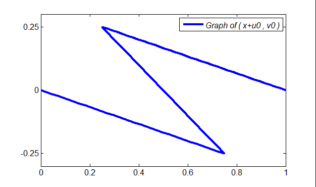
Figure 14: The graph of $(x+u_{0},v_{0})$ for the doubly kinked string.

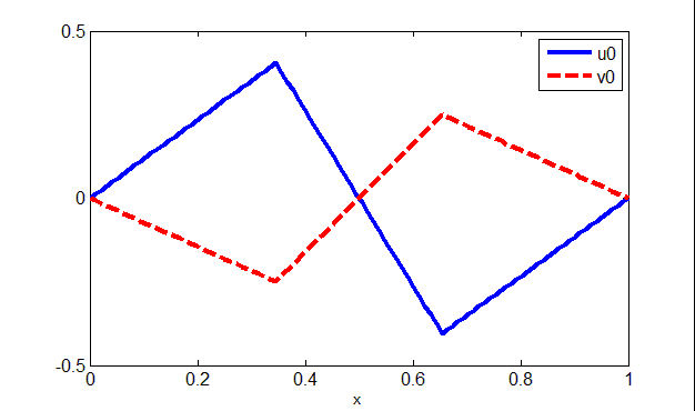
Figure 15: Displacement fields for a doubly kinked string.

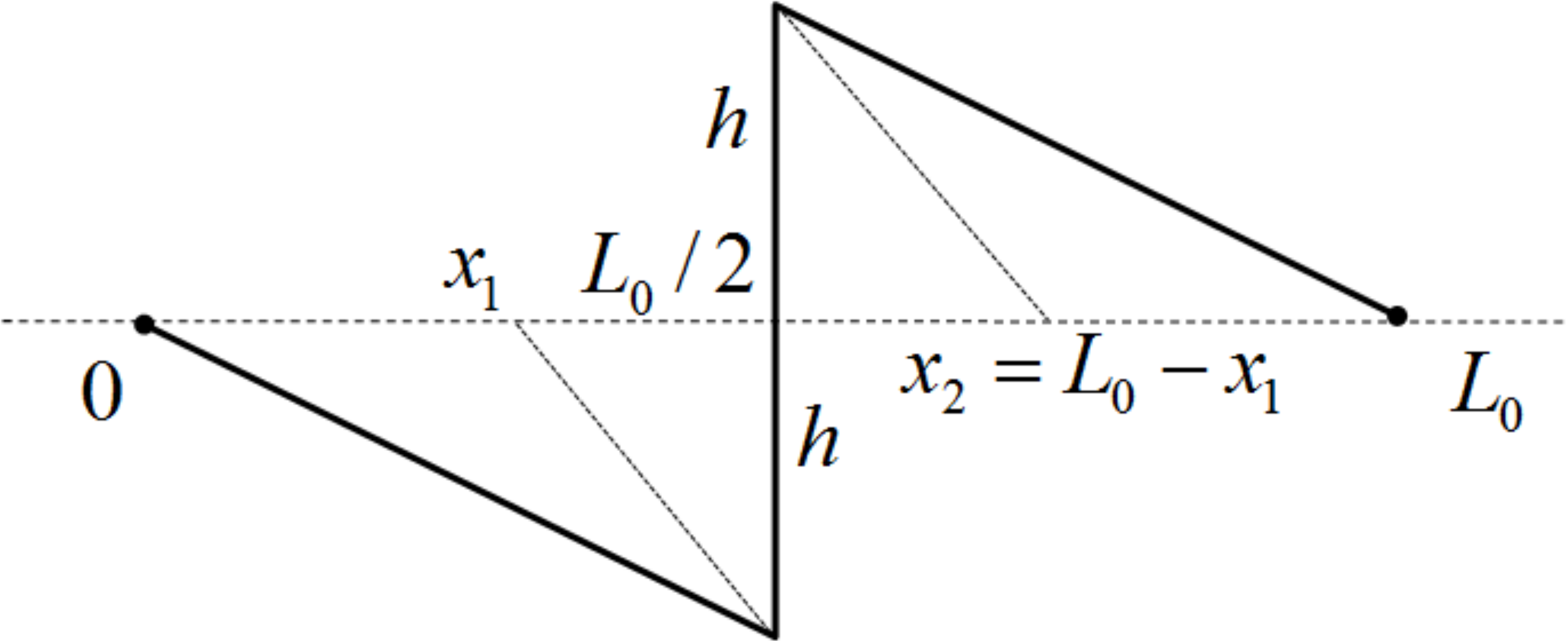
Figure 16: String with an initial double kink and infinite slope at midpoint.

The doubly kinked initial shape shown in Figure 14 is presented as another interesting case, which the classical model has no way of representing. A general case of initial displacement gradients is shown in Figure 15. A particular case is given in Figure 16. The string is allowed to equalize the tension everywhere. Therefore, the extension ratio is constant everywhere in the string. Performing similar analyses as was done above, we obtain the following initial conditions.

$$u_{0}\left(x\right)=\left\{\begin{array}[c]{ccc}\frac{\frac{L_{0}}{2}-x_{1}}{x_{1}}x&&0\leq x\leq x_{1}\\ \frac{L_{0}}{2}-x&&x_{1}\leq x\leq L_{0}-x_{1}\\ -\frac{\left(\frac{L_{0}}{2}-x_{1}\right)\left(L_{0}-x\right)}{x_{1}}&&L_{0}-x_{1}\leq x\leq L_{0}\end{array}\right.$$ (88)

$$v_{0}\left(x\right)=\left\{\begin{array}[c]{ccc}-\frac{h}{x_{1}}x&&0\leq x\leq x_{1}\\ \frac{h\left(2x-L_{0}\right)}{L_{0}-2x_{1}}&&x_{1}\leq x\leq L_{0}-x_{1}\\ \frac{h}{x_{1}}\left(L_{0}-x\right)&&L_{0}-x_{1}\leq x\leq L_{0}\end{array}\right.$$ (89)

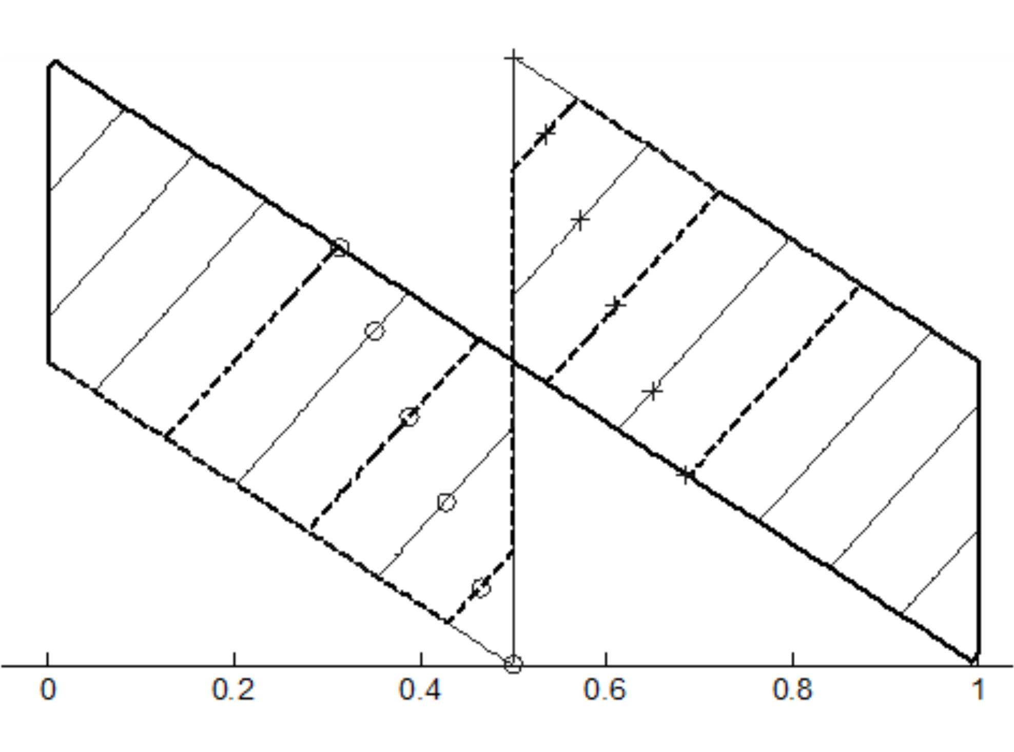
Figure 17: Motion of initially doubly kinked string. Case: $k=0$.

Figure 17 shows the results of numerical analysis for half a period. The thick solid line is the shape at the end of half a period. The motion closely follows Euler’s solutions. All points move along parallel, non-vertical lines and exhibit the characteristic dwelling on envelopes. The midpoint is a vibration node.

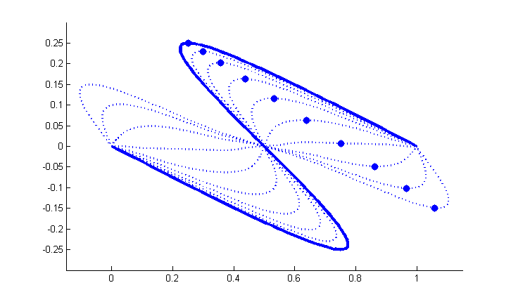
Figure 18: A smoothed double kink solution. The initial conditions were $u_{0}=0.5\sin(2\pi x)$ and $v_{0}=-0.25\sin(2\pi x)$.

Figure 18 shows the solutions to initial conditions approximating a sharp double kink with a smoothed one. The result is obtained with surprisingly simple functions for $u_{0}$ and $v_{0}$.

VI.3 Non-taut string

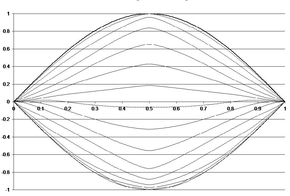
Figure 19: Motion of a string that was non-taut and non-slack at rest.

Figure 19 shows a numerical solution to the general equation for an initially non-taut, non-slack string. The initial conditions were a half sine wave for the shape and zero initial velocity. The numerical solver seems to be reliable since it approaches well to a half sine wave in the negative region even after numerous iteration steps in time. The shape of the curve near zero line deviates significantly from a sine function, which, however, is perfectly recovered at the end of  half period.

VI.4 Twisted loop: a self-intersecting shape

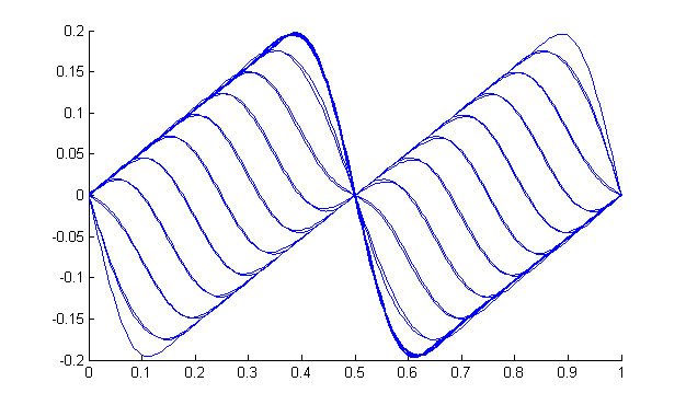
Figure 20: Horizontal motion for the twisted loop initial condition. The darker curve corresponds to $u_{0}$ and $u(x,T/2)$, where $T$ is the period.

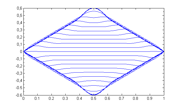
Figure 21: Vertical motion for the twisted loop initial condition. The darker curve corresponds to $v_{0}$ and $v(x,T/2)$, where $T$ is the period

Another interesting initial condition is obtained by the initial conditions depicted in figures 20 and 21. The graph of these is given in Figure 22. The string is allowed to self-intersect. It is interesting that the period of $u(x,t)$ is half those of $v(x,t)$ and the graphed motion. The formation of kinks in the string shape is due to tangent points of lines with the circle in the initial conditions, at which there are curvature discontinuities. These solutions are based on the case of $k=0$. The Euler solutions for individual wave equations and finite element based solutions were both obtained for comparison. They were identical up to numerical accuracies.

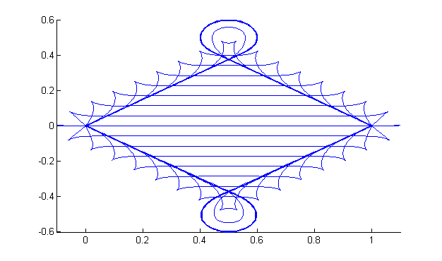
Figure 22: 2D motion for the twisted loop initial condition. The darker curves correspond to the initial shape and the shape after half a period.

VII HIGH-SPEED CAMERA EXPERIMENTS

In order to demonstrate the soundness of the theory and the numerical investigations, a real experiment is conducted using everyday items, except for a high-speed camera.

For the string a common round elastic string with latex fibers is used, which proved to be less than ideal due to its high internal damping. Nevertheless, the first few milliseconds of the motion were sufficient to make a point, at least qualitatively.

The string was stretched between two strong posts approximately 2500 mm apart as measured from the boundaries of the string. A white marker is applied to a small portion of the string, 843 mm from the left end (with respect to the camera), which was used to trace the motion of a material point. The string was pulled up and dragged horizontally away from the left end such that it was displaced by about 100 mm in both directions. Then, the camera was turned on and the string was released.

The camera used was SpeedCam (MiniVis #00655 v1.7.36) with a resolution of 640x512 pixels. The video capture speed was 200 Hz (fps), corresponding to a period of 5 ms.

The resulting image frames were then analyzed using image processing techniques. The first 21 frames after the start of motion were processed. The first frame was used as a substrate onto which the consequent ones were superposed after removing the string image except the marker (Figure 23).

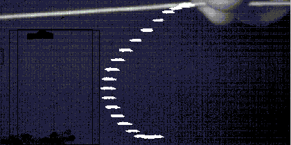
Figure 23: Motion of the marker in the first 105 ms.

A full motion trace was also performed in order to indicate the effect of damping (Figures 24 and 25). The horizontal motion decayed much faster then the vertical motion, due to its faster speed.

In order to be able to compare the experimental results to those obtained from numerical analyses viscous damping terms were introduced to both PDEs. The damping ratios and coefficient were estimated from the camera experiments. Under these conditions the results of the experiment seemed to be quite similar to those of the numerical except for the fact that the real string followed a smoother path. This is due to the effect of bending that was neglected in numerical experiments.

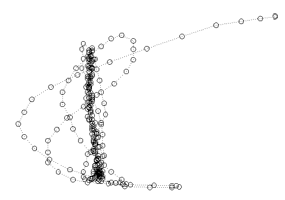
Figure 24: Full trace of the marker in camera experiment.

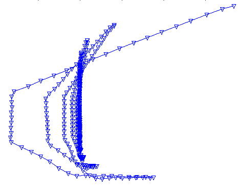
Figure 25: Full trace of the marker in numerical solutions.

As for the other parameters, the following are measured, albeit roughly.

Diameter:	$2.6$ mm
Linear density:	$4.14\times 10^{-3}$ kg/m
Volumetric density:	$779$ kg/m3
Spring constant:	30 N/m
Elastic Modulus:	3.5 MPa
$T_{f}$ and $T_{0}$:	18.5 N and 2.3 N
$k$:	0.89
$c_{f0}$:	71 m/s

The frequency of horizontal motion is measured as 10.5 Hz, whereas that for the vertical was about 5.2 Hz. The horizontal motion was almost twice as fast as the vertical, as was observed in numerical experiments. Whether or not this was a numerical artifact could not be ascertained.

VIII CONCLUSION

It is shown that the classical vibrating string model is not defendable due to lack of accounting for horizontal motions, which are unavoidable except in extremely rare situations. A new 2D motion model, as a pair of non-linear PDEs, is developed in order to account for such shortcomings. Model allows a variety of initial conditions that have no counterparts in the classical model. The most important features of the model are: a) finite displacements, b) variable tension and length, c) reduction to the classical model and others in limit cases, d) handling of previously indescribable cases of non-taut/non-slack strings, self-intersecting shapes, and so on.

Another new result is the determination of initial displacement gradients for strings that are initially allowed to have uniform tension. It is also shown that pure transverse motions are possible only when the string has zero cross-sectional area or zero elastic modulus, the initial tension is uniform (i.e. zero initial horizontal forces), and the initial shape is formed by straight segments around kink points such that the segment slopes on each side of kinks are equal and opposite.

Various numerical experiments are conducted on different platforms for verification of the analytic models, which seem to agree with each other to a high degree of accuracy. High-speed camera experiments were conducted that seemed to unequivocally support the new theory.

IX REFERENCES

References

- (1) D’Alembert, J. L. (1747). Recherches Sur la Courbe Que Forme Une Corde Tenduë Mise en Vibration. Hist. de l’Acad. Roy. de Berlin, 3, pp. 214-219.
- (2) D’Alembert, J. L. (1747). Suite des Recherches Sur la Courbe Que Forme Une Corde Tenduë Mise en Vibration. Hist. de l’Acad. Roy. de Berlin, 3, pp. 220-249.
- (3) Euler, L. (1748). Sur la Vibration des Cordes. Hist. de l’Acad. Roy. de Berlin, 4, pp. 69-85.
- (4) Bernoulli, D. (1732/1733). Theoremata de Oscillationibus Corporum Filo Flexili Connexorum et Catenae Verticaliter Suspensae. Comentarii Academiae Scientiarum Imperialis Petropolitanae, 6, pp. 108-122.
- (5) Bernoulli, D. (1740). De Oscillationibus Composites Praesertim Iss Quae Flunt in Corporibus Ex Filo Flexili Suspensis. Comentarii Academiae Scientiarum Imperialis Petropolitanae, 12, pp. 97-108.
- (6) Bernoulli, D. (1753). Réflexions et Éclaircissemens Sur les Nouvelles Vibrations des Cordes. Hist. de l’Acad. Roy. de Berlin, 9, pp. 147-195.
- (7) Bernoulli, J. (1728). Meditationes de Chordis Vibrantibus. Comentarii Academiae Scientiarum Imperialis Petropolitanae. 3, pp. 13-28. (Translated by NASA: Deliberations On Oscillating Strings, NASA TT F-9515, 1965)
- (8) Fourier, J. B. (1819). Théorie du Mouvement de la Chaleur Dans les Corps Solides. Mém. de l’Acad. Roy. des Sci. de l’Inst. de France, 4, pp. 185-556.
- (9) Dirichlet, P. G. (1829). Sur la Convergence des Séries Trigonométriques Qui Servent À Représenter Une Fonction Arbitraire Entre des Limites Données. J. für Math., 4, 157-169. Retrieved from arXiv:0806.1294v1.
- (10) Wheeler, G. F. and Crummett, W. P. (1987). The Vibrating String Controversy. Am. J. Phys., 55(1), 33-37.
- (11) Zeeman, E. C. (1993). Controversy in Science: on the Ideas of Daniel Bernoulli and René Thom. Nieuw Arch. Wisk. (4), 11(3), pp. 257-282.
- (12) Armstead, D. C. and Karls, M. A. (2006). Does the Wave Equation Really Work?, PRIMUS, 16 (2), pp. 162-177. http://dx.doi.org/10.1080/10511970608984144.
- (13) Benson, D. J., Music: A Mathematical Offering, 2007, Cambridge University Press, UK and USA.
- (14) Byron, F. W. and Fuller, R. W., Mathematics of Classical and Quantum Physics, 1992, Dover Pub. (Original publications, 1969, 1970: General Publishing Co., Canada; and Constable and Company, UK).
- (15) Ciblak, N. (2013). Arbitrarily Large Motion Model For Transverse Vibrations of a String. arXiv:1310.1019v1.
- (16) Gottlieb, H. P. W., (1990), Non-linear Vibration of a Constant-Tension String, J. Sound Vib., v. 143, pp 455-460.
- (17) Kreysig, E., Advanced Engineering Mathematics, 1983, New York: John Wiley and Sons, 5th ed.
- (18) Lagrange, J.-L. (1759). Recherches Sur la Nature et la Propagation du Son. Miscell. Taurin., 1, pp. 39-148.
- (19) Lai, S. K., Xiang, Y., et al., 2008, Higher-Order Approximate Solutions For Non-linear Vibration of a Constant-Tension String, J. Sound Vib., v.317, pp 440-448.
- (20) Powers, D. L., Boundary Value Problems. New York: Saunders College, 3rd ed.
- (21) Rao, G. V., 2002, Moderately Large Amplitude Vibrations of a Constant Tension String: a Numerical Experiment, J. Sound Vib., v. 263, pp 227-232.
- (22) Sagan, H., Boundary and Eigenvalue Problems in Mathematical Physics, 1989, Dover Pub. (Original publication, 1961, Wiley)
- (23) Taylor, B. (1713). De Motu Nervi Tensi. Phil. Trans., 28, pp. 26-32.
- (24) Weinstock, R., Calculus of Variations, 1974, Dover Pub. (Original publications, 1952: General Publishing Co., Canada; and, Constable and Company, UK)