An acoustical analogue of a galactic-scale gravitational-wave detector

Abstract

By precisely monitoring the “ticks” of Nature’s most precise clocks (millisecond pulsars), scientists are trying to detect the “ripples in spacetime” (gravitational waves) produced by the inspirals of supermassive black holes in the centers of distant merging galaxies. Here we describe a relatively simple demonstration that uses two metronomes and a microphone to illustrate several techniques used by pulsar astronomers to search for gravitational waves. An adapted version of this demonstration could be used as an instructional laboratory investigation at the undergraduate level.

I Introduction

A pulsar timing array is a galactic-scale gravitational-wave detector, which can be used to search for gravitational waves from the inspiral of supermassive black-hole binaries (of order $10^{9}$ solar masses) in the centers of distant galaxies(Bizouard et al., 2013; Detweiler, 1979; Hellings & Downs, 1983). The array consists of a set of galactic millisecond pulsars—rapidly-rotating neutron stars, which have masses of order the mass of the Sun and magnetic fields of order a billion times stronger than that of the Earth(Lorimer & Kramer, 2012). Millisecond pulsars rotate nearly a thousand times each second (faster than a kitchen blender), emitting a narrow beam of radio waves along the magnetic axes that sweep across the sky similar to a revolving beacon on top of a lighthouse. If this radio beam crosses our line of sight to the pulsar, a radio telescope on Earth will observe pulses of radiation, which arrive with a regularity that rivals (or even exceeds) that of the best atomic clocks(Hobbs et al., 2012).

By precisely monitoring the pulse arrival times, radio astronomers can determine what the rotation period of the pulsar is, how the rotation is slowing down, whether the pulsar is orbiting a companion star, as well as how the interstellar medium affects the propagation of the pulses(Lorimer & Kramer, 2012). The difference between the measured times of arrival and the expected times of arrival (taking all of these effects into account) are called timing residuals. If the pulsar timing model is good, the residuals should be randomly scattered around zero with a root-mean-square (rms) amplitude determined by measurement noise in the radio receiver and statistical fluctuations in the pulses themselves. The residuals for an individual pulsar may be correlated in time(Cordes & Downs, 1985; Lentati et al., 2016; Lam et al., 2017; Cordes, 2013) (so-called red noise), but residuals associated with different Earth-pulsar baselines should not be correlated with one another in the absence of any common external influence. Deviations from this expected behavior could be due to either an incomplete timing model (e.g., not realizing that the pulsar is in a binary) or the presence of gravitational waves(Condon & Ransom, 2016).

A gravitational wave passing between the Earth and a pulsar will stretch and squeeze space transverse to its motion, slightly advancing or retarding the arrival times of the individual pulses(Estabrook & Wahlquist, 1975). Unlike the measurement noise or intrinsic pulsar timing noise discussed above, the modulation of pulse arrival times induced by a gravitational wave will be correlated across different pulsars in the array, due to its common influence in the vicinity of the Earth. Moreover, this correlation will have a very specific dependence on the angle between a pair of Earth-pulsar baselines, the so-called Hellings and Downs curve(Hellings & Downs, 1983) shown in Figure 1.

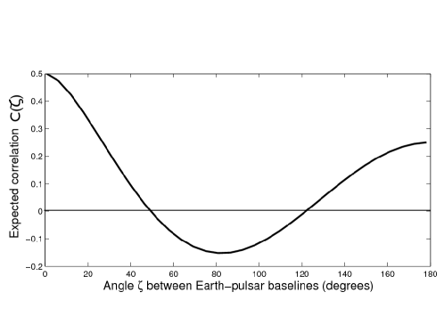
Figure 1: Expected correlation coefficient between the timing residuals for a pair of Earth-pulsar baselines separated by angle $\zeta$.

The detection of this expected correlation in the timing residuals from an array of pulsars would be evidence for the presence of gravitational waves, similar to the recent detections by the advanced LIGO and Virgo detectorsAbbott et al. (2016); LIGOPapers ; Abbott et al. (2017).

I.1 Metronomes and microphones

In order to illustrate how gravitational-wave astronomers are using correlation methods to search for gravitational waves, we have developed a demonstration using metronomes and a microphone, which serves as an acoustical analogue of a pulsar timing array. In this demonstration, radio pulses from an array of Galactic pulsars are represented by ticks of an array of metronomes (only two metronomes are needed for this demonstration); radio receivers on Earth are represented by a single microphone; and the passage of a gravitational wave is represented by the motion of the microphone around its nominal position. The analogy is not perfect as the motion of the microphone does not represent a wave of any kind, and the correlations that it induces have a different angular dependence than that induced by a real gravitational wave(Jenet & Romano, 2015). But what is important is that there are correlations, as the microphone motion modulates the arrival times of the metronome pulses by changing the distance between the metronomes and the microphone. And although the angular dependence of the correlations for the microphone motion is different than that for gravitational waves, it is, nonetheless, a specific function of the angle between a pair of microphone-metronome baselines, which can be calculated theoretically and also verified experimentally by doing the demonstration.

In the following sections, we will describe the metronome-microphone demonstration in detail. In Section II, we describe the specific hardware (i.e., metronomes and microphone) and software routines that we use to do the analysis. In Section III, we list the techniques used in real pulsar timing analyses that are illustrated by the demonstration. They can be thought of as the learning outcomes for the demonstration. In Sections IV and V, we discuss the two main parts of the demonstration (the single-metronome and double-metronome analyses), listing the steps needed to perform the analysis and the function of the graphical user interface (GUI) buttons used to execute each step. In Section VI, we conclude with a discussion of some caveats and possible improvements to the demonstration, and how it might be adapted for use in the collection of high school and undergraduate laboratory(Rubbo et al., 2007; Newburgh, 2008; Ford et al., 2015; Burko, 2017) and classroom(Farr et al., 2012; Kassner, 2015; Mathur et al., 2017; Kaur et al., 2017; Hilborn, 2018) investigations centered around understanding gravitational physics. [Sample data files and analysis routines are available for download from URL http://github.com/josephromano/pta-demo.]

II Required hardware and software

The metronome-microphone pulsar-timing-array demonstration requires two metronomes. Our preferred choice is Seiko model SQ50-V quartz metronomes (Figure 2), as this model has adjustable beats-per-minute (bpm) up to 208 bpm, adjustable volume, and two different tempo sounds—mode $a$ and mode $b$, with mode $b$ having a slightly higher pitch. Having two modes is helpful in distinguishing the pulses from the individual metronomes when both metronomes are on simultaneously, since the pulse shapes (profiles) are different.

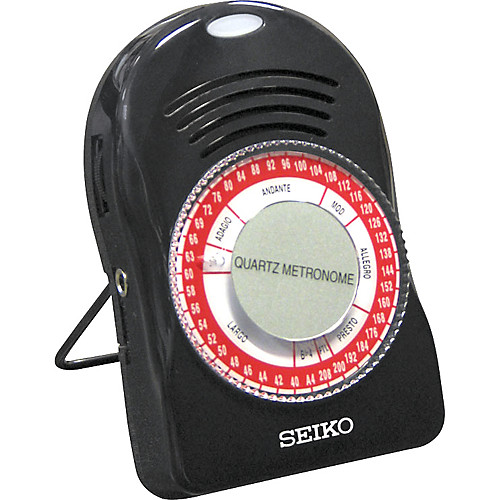
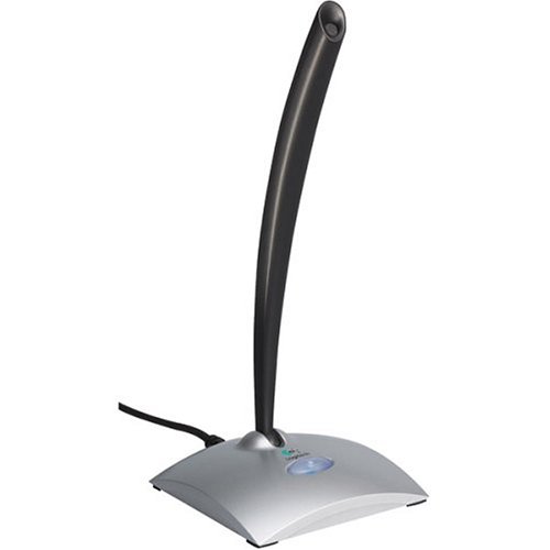
Figure 2: Two Seiko metronomes and one Logitech USB noise-canceling microphone used for the demonstration.

One also needs some type of microphone, either an external USB microphone or an internal microphone, connected to a laptop that is set up to run the relevant data analysis routines (described below). We have found that the internal microphone on a MacBook Pro works best since it has ambient noise reduction, although it is somewhat inconvenient to physically move the laptop to simulate the passage of a gravitational wave. (We move the microphone is a small circle of radius $\sim\!10~{}{\rm cm}$ at constant speed, for reasons we will describe below.) We have also used a Logitech USB Desktop noise-canceling microphone (Figure 2), which is a little easier to maneuver.

In addition, one needs an open space covering an area of about $10~{}{\rm ft}\times 5~{}{\rm ft}$ for the placement of the two metronomes and microphone. A schematic diagram of the setup is shown in Figure 3. A photograph of an actual real-world setup used to take the data is shown in Figure 4.

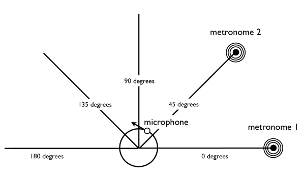
Figure 3: Schematic diagram showing the location of the microphone and metronomes for the different analyses. The stationary microphone is located at the origin; the moving microphone undergoes uniform circular motion, indicated by the counter-clockwise circle. Metronome 2 is placed at angular location $45^{\circ}$ in this figure, but will be placed at the other angular locations for different parts of the demonstration.

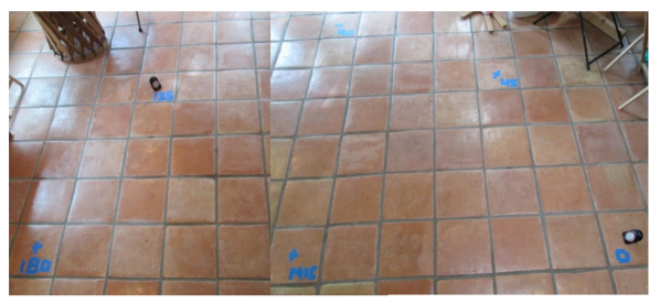
Figure 4: Photograph of an actual setup for data taking. Metronome 1 is shown at angular location $0^{\circ}$; metronome 2 at angular location $135^{\circ}$. The separation between the microphone (located at the origin) and the metronomes at the edge of a semi-circle is approximately 5 feet.

We have written Python-based routines to do the relevant data analysis calculations. These includes routines for: (i) audio recording and play back of metronome pulses, (ii) pulse data folding, (iii) pulse profile calculation, (iv) matched-filter estimation of pulse arrival times, (v) timing residual calculation, (vi) linear detrending of timing residuals, (vii) fitting of sinusoids to the timing residuals, and (viii) correlation coefficient calculation. Two Python-based GUIs exist for performing the two main data taking and data analysis tasks: PTAdemo1GUI.py (for analyzing the single-metronome data) and PTAdemo2GUI.py (for analyzing the double-metronome data). The two GUIs and the data analysis techniques are described in more detail in the following sections.

III Pulsar timing techniques illustrated by the demonstration

The metronome-microphone demonstration is useful as an educational tool since it illustrates several techniques used in real pulsar timing analyses. It does this in the simplified context of metronome pulses recorded by a microphone, which students or the general public can more easily identify with. To set the stage for the analyses that will be described in Secs. IV and V, we describe below the key techniques illustrated by the demonstration.

III.1 Folding data

Folding data is a technique that can be used to find both the pulse period and pulse shape (profile) in noisy time-series data (Lorimer & Kramer, 2012). The time-series (of total duration $T_{\rm tot}$) is first split into smaller segments, each of duration $T$, which are then averaged together. If $T$ matches the true pulse period $T_{\rm p}$, then the pulse contributions in each segment combine coherently when the segments are summed, while the noise contributions combine incoherently (positive and negative values tending to cancel one another). If $T$ does not match the true pulse period, the pulse contributions will effectively cancel out when averaged against the noise. So the basic procedure is to systematically try different values of $T$ until a pulse profile “sticks out of the data”, which will occur when $T$ equals $T_{\rm p}$. The signal-to-noise ratio of the recovered pulse profile grows like $\sqrt{N}$, where $N$ is the number of segments or, equivalently, the number of individual pulses combined(Cordes & Shannon, 2010). Figure 5 illustrates what happens when you fold data with an incorrect and the correct pulse period.

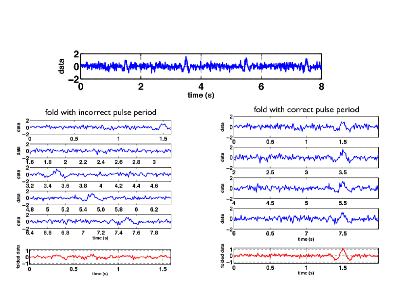
Figure 5: Illustration of folding data with both an incorrect and the correct choice for the pulse period $T_{\rm p}$. Top panel: Noisy time-series data with several injected pulses having $T_{\rm p}=2~{}{\rm s}$. Left column: Segments of the original time-series data each of duration $1.6$ s (in blue), and the average of these segments (in red). Right column: Same as for the left column but for segments of duration 2 s. Note that when the data are folded with the correct pulse period $T_{\rm p}=2~{}{\rm s}$, the signal components combine coherently and the pulse profile is easily visible in the average of the segments (bottom right plot).

III.2 Matched-filter determination of pulse arrival times

The measured times of arrival (TOAs) are determined by correlating a time-shifted version of the pulse profile with the time-series data(Taylor, 1992; Lam et al., 2016). Mathematically, one calculates the correlation function

$$C(\tau)\equiv{\cal N}\int dt\>y(t)p(t-\tau)\,,$$ (1)

where $y(t)$ is the timeseries and $p(t-\tau)$ is the pulse profile shifted forward in time by $\tau$. (${\cal N}$ is a normalization constant, defined below.) In the frequency domain, we have

$$C(\tau)={\cal N}\int df\>\tilde{y}(f)\tilde{p}^{*}(f)e^{i2\pi f\tau}\,,\qquad{\cal N}\equiv\left[\int df\>|\tilde{p}^{*}(f)|^{2}\right]^{-1}\,,$$ (2)

where $\tilde{y}(f)$ and $\tilde{p}(f)$ are the Fourier transforms(FourierFootnote, ) of $y(t)$ and $p(t)$. The correlation function $C(\tau)$ has local maxima at the arrival times of the pulses (Figure 6).

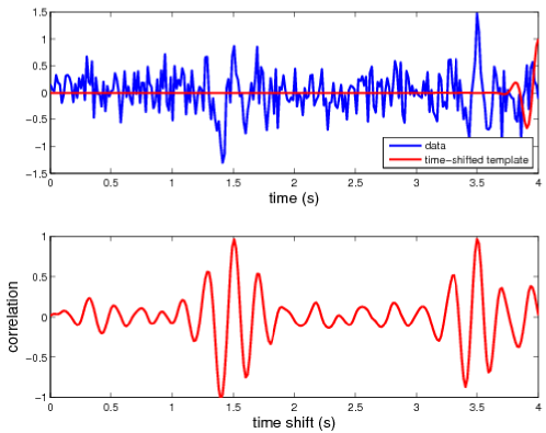
Figure 6: Illustration on simulated data showing that how the correlation function $C(\tau)$ has local maxima at the arrival times of the pulses. An animation showing the calculation of $C(\tau)$ as a function of the timeshift of the pulse profile is available at http://github.com/josephromano/pta-demo/tree/master/code/, with filename matchedfilterdemo.avi.

In what follows, we will denote these measured arrival times by $\tau^{\rm meas}[i]$, where $i=1,2,\cdots$. The normalization constant ${\cal N}$ is included so that the values of the correlation function at the measured TOAs are estimates of the amplitudes of the pulses.

III.3 Calculating timing residuals based on a timing model

Calculating the timing residuals is a simple matter of subtracting the expected TOAs from the measured TOAs of the pulses:

$$\delta\tau[i]=\tau^{\rm meas}[i]-\tau^{\rm exp}[i]\,,$$ (3)

where $i=1,2,\cdots$ labels the individual pulses. As mentioned in Sec. I, for real pulsar timing analyses the expected TOAs are determined by a rather sophisticated timing model, which takes into account the rotation period of the pulsar, its spin-down rate, its location in the sky, etc. But for the metronome-microphone demonstration, the timing model is exceedingly simple:

$$\tau^{\rm exp}[i]=\tau^{\rm meas}[i_{0}]+(i-i_{0})T_{\rm p}\,,$$ (4)

which is just the measured TOA of the pulse having the largest correlation with the pulse profile, indexed by $i_{0}$, plus integer multiples of the pulse period $T_{\rm p}$ of the metronome.

III.4 Improving the timing model by removing a linear trend in the residuals

A linear trend in the timing residuals is an indication that the pulse period (determined by folding the data in Step 1 above) is not quite right. This is because $\delta\tau[i]$ involves a term $-(i-i_{0})T_{\rm p}$, and if there is an error $\epsilon$ in $T_{\rm p}$, this term grows linearly with the pulse number, $i$. By fitting a line to the timing residuals and removing this trend, we obtain an improved estimate of the pulse period, which we can be used for subsequent timing model calculations. Figure 7 show timing residuals for metronome pulses before and after removing a linear trend.

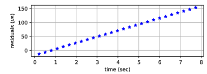
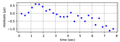
Figure 7: Residuals for metronome pulses: (a) before detrending, and (b) after detrending. Note the different scales on the $y$-axis.

III.5 Calculating correlation coefficients between pairs of timing residuals

The correlation coefficient between a pair of timing residuals is simply the time-averaged product of the timing residuals for a pair of microphone-metronome baselines. More generally, we can define the binned correlation function

$$C_{12}[k]\equiv\frac{1}{N_{\rm bins}}\sum_{i,j}\delta\tau_{1}[i]\delta\tau_{2}[j]\,,$$ (5)

$$\forall i,j\quad{\rm s.t.}\quad\tau^{\rm meas}_{1}[i]-\tau^{\rm meas}_{2}[j]\in\left[k-0.5,k+0.5\right]\Delta t\,,$$

for two sets of timing-residuals $\delta\tau_{1}$, $\delta\tau_{2}$, where $\Delta t$ is the chosen bin size. (The condition on the indices $i$ and $j$ is simply that the difference in the measured times of arrival for the two timing residuals must lie in the $k$th lag bin.) But for the purposes of the demonstration: (i) we are interested in only the zero-lag result (so $k=0$), and (ii) to simplify the calculation, we can fit smooth curves $x_{1}(t)$, $x_{2}(t)$ to the two sets of timing residuals, for which

$$C_{12}[0]\quad\rightarrow\quad\langle x_{1}x_{2}\rangle\equiv\frac{1}{T_{\rm tot}}\int_{0}^{T_{\rm tot}}dt\>x_{1}(t)x_{2}(t)\,.$$ (6)

Normalizing by the rms values $\sqrt{\langle x_{1}^{2}\rangle}$ and $\sqrt{\langle x_{2}^{2}\rangle}$, we get

$$\left.\rho_{12}\equiv{\langle x_{1}x_{2}\rangle}\right/\sqrt{\langle x_{1}^{2}\rangle\langle x_{2}^{2}\rangle}\,,$$ (7)

for the correlation coefficient, which takes values between $-1$ and 1. Note that for timing residuals induced by uniform circular microphone motion (see Secs. III.7 and III.8), the best-fit smooth functions to the timing residuals will be sinusoids.

III.6 Microphone-motion-induced timing residuals

Similar to calculating the response of an Earth-pulsar baseline to a passing gravitational wave, one can calculate the response of a metronome timing residual to the motion of the microphone:

$$\delta\tau_{I}^{\rm mic}(t)\equiv\frac{\Delta L_{I}(t)}{c_{\rm s}}=\frac{L_{I}(t)-L_{I}}{c_{\rm s}}\simeq-\frac{1}{c_{\rm s}}\hat{u}_{I}\cdot\vec{r}(t)$$ (8)

where $L_{I}(t)$ is the distance between metronome $I=1,2$ and the location of the microphone $\vec{r}(t)$ at time $t$, $L_{I}$ is the nominal distance between the metronome and the microphone pointing in direction $\hat{u}_{I}$, and $c_{\rm s}$ is the speed of sound in air. This response is just the change in the metronome pulse propagation time due to the motion of the microphone relative to metronome $I$. The last (approximate) equality above is valid if we ignore correction terms of order $A/L\sim 0.1$, where $A\sim 10~{}{\rm cm}$ is the amplitude of the microphone motion and $L\sim 1~{}{\rm m}$ is the distance from the metronome to the microphone when it is at the origin. Such an approximation amounts to ignoring the curvature of the pulse wavefronts.

III.7 Expected correlations in the timing residuals induced by uniform circular motion

For the microphone undergoing uniform circular motion with amplitude $A$ and frequency $f_{0}$,

$$\vec{r}(t)=A\left[\cos(2\pi f_{0}t+\phi_{0})\,\hat{x}+\sin(2\pi f_{0}t+\phi_{0})\,\hat{y}\right]\,,$$ (9)

it follows immediately that

$$\delta\tau_{I}^{\rm mic}(t)\simeq-\frac{A}{c_{\rm s}}\cos(2\pi f_{0}t+\phi_{0}-\theta_{I})\,,$$ (10)

where $\theta_{I}$ is the angle that the location of metronome $I$ makes with respect to the $x$-axis, and where (as before) we have ignored the higher-order correction terms to the residual. Using the trigonometric identity

$$\cos A\cos B=\frac{1}{2}\left[\cos(A+B)+\cos(A-B)\right]\,,$$ (11)

it is fairly easy to show that the time-averaged correlation coefficient of the microphone-induced timing residuals for metronomes 1 and 2 is

$$\rho_{12}\simeq\cos\zeta\,,$$ (12)

where $\zeta\equiv\theta_{1}-\theta_{2}$ is the angle between the two microphone-metronome baselines. This equality is correct to order $(A/L)^{2}$. This dependence of the correlation coefficient on the angle between the two metronomes is what we confirm experimentally with the double-metronome analysis described in Sec. V. Since the timing residuals for the two metronomes typically are evaluated at different times, we actually correlate the best-fit sinusoids to the timing residuals, as described in Sec. III.5.

III.8 Justification of the choice of uniform circular motion for the microphone

In principle, we could move the microphone in any way whatsoever, and we would still see correlations in the timing residuals associated with the two metronomes. But the form of the expected correlation will be more complicated than the simple $\rho_{12}\simeq\cos\zeta$ dependence that we found above. For example, if instead of uniform circular motion we let the microphone swing back-and-forth sinusoidally in a plane (i.e., along some line in the $xy$-plane), then the correlation coefficient will also depend on the angle that this plane makes with the $x$-axis. Said another way, uniform circular motion has the nice property that the $x$ and $y$ components of its motion are statistically equivalent, but uncorrelated with one another. It turns out that this is also the assumption that goes into the calculation of the Hellings and Downs correlation curve (Figure 1) for the real pulsar-timing gravitational-wave case—i.e., the Hellings and Downs curve is derived under the assumption that the pulsar timing array is responding to a stochastic background of gravitational waves that is both isotropic (no preferred direction) and unpolarized (statistically equivalent and uncorrelated linear polarization components)(Hellings & Downs, 1983).

From a different perspective, the effect of uniform circular motion on the timing residuals is exactly what one sees in real pulsar-timing timing residuals if the yearly orbital motion of the Earth around the Sun is not taken into account in the timing models for the pulsars.

IV Single-metronome analysis

The purpose of the single-metronome analysis is to calculate the pulse period and pulse profile for each metronome separately in the absence of microphone motion. The pulse periods and pulse profiles calculated here can be considered as reference periods and profiles, to be used as inputs for the double-metronome analysis, where both metronomes are running simultaneously and the microphone is moving when it is recording pulses.

A screenshot of the GUI for this analysis, PTAdemo1GUI.py, is shown in Figure 8. The GUI has space for plots of: (i) pulses from the individual metronomes, (ii) pulse profiles (obtained by folding the pulse data), and (iii) timing residuals. The GUI also has several text entry fields and buttons, whose functions are described below:

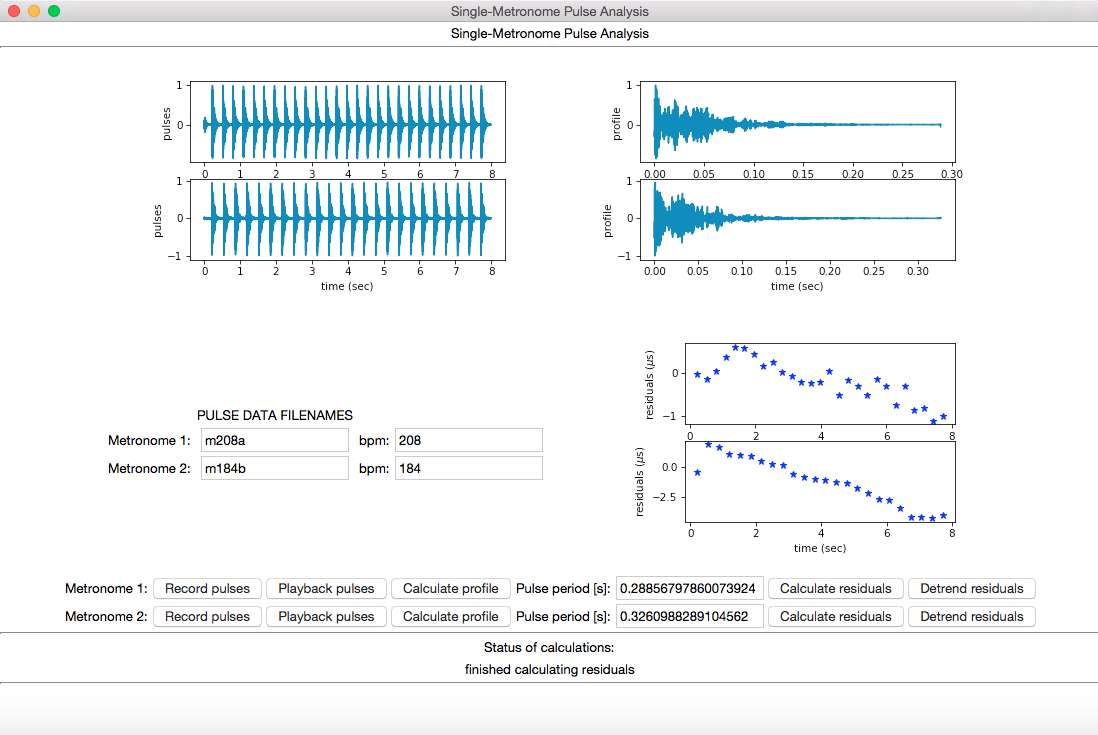
Figure 8: Python GUI for the single-metronome analysis. Plots, text entry fields, and buttons are described in the main text.

Record pulses: Records audio pulse data from a metronome, and save the corresponding timeseries to an ascii .txt file with file prefix specified by the PULSE DATA FILENAMES text entry boxes (default m208a or m184b). The bpm text entry boxes have the beats-per-minute settings for the two metronomes. The pulse recording routine is hard-coded to record 8 seconds of data.

Playback pulses: Plays back and plots the audio pulse data saved in the ascii files, again defaulted to m208a.txt or m184b.txt.

Calculate profile: Either (i) calculates the pulse period $T_{\rm p}$ and pulse profile directly by folding the metronome data, and then saves the profile to the file m208a_profile.txt or m184b_profile.txt, or (ii) reads in the pulse profile data that has already been saved in these files. Method (i) is used only the first time the analysis is run. If the pulse profiles are read-in from the files m208a_profile.txt and m184b_profile.txt, the text entry boxes for the pulse periods need to be entered by hand. For both cases, the pulse profile is plotted from 0 to $T_{\rm p}$.

Calculate residuals: Calculates the timing residuals by subtracting the expected TOAs from the measured TOAs of the pulses as described in Secs. III.3 and III.2.

Detrend residuals: Improves the estimate of the pulse period for a metronome by removing a linear trend from the timing residuals as described in Sec. III.4. Detrending may change the estimate of the pulse period by 1-2 microseconds. The updated period is displayed in the Pulse period text entry box.

IV.1 Steps for doing the analysis

1. Record pulses from each metronome separately, keeping the microphone stationary. The microphone should be located at the origin of coordinates and the two metronomes should be at angular location $0^{\circ}$. The file prefixes and bpms in the text entry boxes should be chosen to match the physical settings of the metronome.

2. After recording the pulse data for each metronome, you can play it back, calculate the corresponding pulse profile and period, calculate the residuals, and detrend the residuals, by simply pressing the relevant GUI buttons.

This analysis produces two pulse profile data files (e.g., m208a_profile.txt and m184b_profile.txt) and the associated pulse periods for the two metronomes, which are needed for the double-metronome analysis described in the next section.

V Double-metronome analysis

The purpose of the double-metronome analysis is to experimentally verify the expected $\rho_{12}\simeq\cos\zeta$ correlation coefficient for the timing residuals for the two metronomes when the microphone is undergoing uniform circular motion. This is analogous to real pulsar timing analyses looking for evidence of the Hellings and Downs correlation curve when correlating timing residuals for pairs of Earth-pulsar baselines.

A screenshot of the GUI for this analysis, PTAdemo2GUI.py, is shown in Figure 9. The GUI has space for plots of: (i) pulses from the two metronomes running simultaneously, (ii) reference pulse profiles for the two metronomes, which were calculated using PTAdemo1GUI.py, and (iii) timing residuals for the two metronomes. The GUI also has several text entry fields and buttons, whose functions are described below:

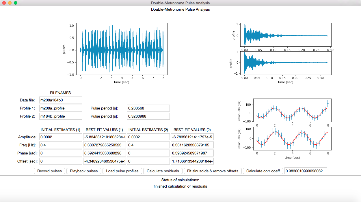
Figure 9: Python GUI for the double-metronome analysis. Plots, text entry fields, and buttons are described in the main text.

Record pulses: Records audio pulse data from the two metronomes running simultaneously, and then saves the corresponding timeseries to an ascii .txt file with file prefix specified by the Data file text entry box under the FILENAMES label (default m208a184b0).

Playback pulses: Plays back and plots the audio pulse data saved in m208a184b0.txt.

Load pulse profiles: Reads-in and plots the reference pulse profiles for the two metronomes, which were calculated by PTAdemo1GUI.py and were saved in ascii .txt files specified by the Profile 1,2 text entry boxes under the FILENAMES label (default m208a_profile and m184b_profile). The text entry boxes for the pulse periods should be filled with in with the values calculated by PTAdemo1GUI.py.

Calculate residuals: Calculates the timing residuals as described previously for PTAdemo1GUI.py.

Fit sinusoids & remove offsets: Simultaneously removes constant offsets and calculates best-fit sinusoids to the timing residuals for the two metronomes, using initial estimates for the amplitude, frequency, and phase of the sinusoids, and the constant offset given in the text entry boxes labeled INITIAL ESTIMATES (1,2) (defaults $2\times 10^{-4}$, $0.4~{}{\rm Hz}$, 0 radians, and 0 sec, respectively). The constant offset arises from the arbitrariness of setting the timing residual of the pulse with the highest correlation to zero. The best-fit parameter values calculated by Fit sinusoids & remove offsets are written to the text entry boxes labeled BEST-FIT VALUES (1,2).

Calculate corr coeff: Calculates the time-averaged correlation coefficient between the best-fit sinusoids for the two sets of timing residuals, as described in Sec. III.5. Theoretically, the value of the correlation coefficient should equally $\cos\zeta$, where $\zeta$ is the separation angle between the line-of-sights to the two metronomes, as described in Sec III.7.

V.1 Steps for doing the analysis

1. Start by placing both metronomes at the same angular location $0^{\circ}$ and at the same distance $L\sim 1~{}{\rm m}$ from the origin. With both metronomes running simultaneously, record the audio data while moving the microphone in uniform circular motion about the origin: Typically, it is best to have $A\approx 10~{}{\rm cm}$ (=0.1 m) and period of oscillation $T_{0}\equiv 1/f_{0}\approx 2~{}{\rm s}$. This leads to microphone-induced timing residuals of order $A/c_{\rm s}\approx 3\times 10^{-4}~{}{\rm s}$, where $c_{\rm s}=340~{}{\rm m/s}$ is the speed of sound in air. This timing precision turns out to be more than an order-of-magnitude larger than the precision to which we can estimate the TOAs of the metronome pulses, meaning that we can easily observe the effect of microphone motion in the timing-residual data.

2. After recording the double-metronome data, you can play it back, load the pulse profiles, and calculate the residuals for each metronome. The timing residuals induced by the microphone motion should be sinusoidal and have large signal-to-noise ratio. You should then fit sinusoids to the residuals for each metronome, adjusting the INITIAL GUESS amplitudes, frequencies, and phases if necessary. (The initial guesses just have to be close, not exact.) Finally, you should calculate the correlation coefficient, which should have a value very close to 1 for this case, since the two microphones are at the same angular location.

3. Repeat the above two steps but with metronome 2 at different angular locations ($45^{\circ}$, $90^{\circ}$, $135^{\circ}$, $180^{\circ}$) with respect to metronome 1 (which should always remain at $0^{\circ}$). The motion of the microphone should be as similar as possible to that for Step 1. Change the name of the file prefix in the Data file text entry box to m208a184bXX, where XX is 45, 90, 135, 180, to reflect the change in the angular location of metronome 2. You should find that the correlation coefficient is approximately equal to $\cos\zeta$, where $\zeta=45^{\circ}$, $90^{\circ}$, $135^{\circ}$, $180^{\circ}$ is the angular separation of the two metronomes.

This analysis produces data files (m208a184bXX.txt, where XX is 0, 45, 90, 135, 180), containing the double-metronome pulse timeseries.

VI Discussion

We have described a demonstration using two metronomes and a microphone that serves as an acoustical analogue of a Galactic-scale gravitational-wave detector, i.e., a pulsar timing array. This demonstration also serves as an educational tool, illustrating several techniques used in real pulsar timing analyses, but in the simplified context of metronome pulses recorded by a microphone. From our experience, we have found that the demonstration is best suited for undergraduates or senior-level high-school students who already have some familiarity with basic physics and astronomy. For less mathematically-inclined audiences, the mathematical discussion of the underlying data analysis techniques needs to be reduced accordingly. But the main idea that a common disturbance (in this case, the microphone motion) can induce correlations in the pulse arrival times, and a graphical display showing the timing residuals from the two metronomes being shifted by an amount equal to their angular separation is accessible to nearly all audiences.

VI.1 Some caveats

The tricky technical aspect of the double-metronome analysis is to properly extract the pulse arrival times when the two metronomes are running simultaneously, producing pulses that can significantly overlap with one another. The fact that the pulse profiles $p_{I}(t)$ for the two metronomes ($I=1,2$) are different for different tempo modes $a$ and $b$ is crucial for distinguishing the pulses from the two metronomes. Still, the correlation functions $C_{I}(\tau)$ have several local maxima, and we need to find the largest local maxima in the vicinity of the expected pulse arrival times to determine the measured TOAs $\tau_{I}^{\rm meas}[i]$. If the search window is not properly centered on the expected arrival time or if it includes a local maximum of the correlation function that doesn’t correspond to the true arrival time of the pulse, then the returned measured TOA will deviate from its true value, thus causing errors in the corresponding timing residual and the subsequent fit to the residuals. To help mitigate such problems, the routine that calculates the measured TOAs currently uses an adaptive width for the search window, which increases in size if it originally does not include a peak in the correlation function (this is usually a sign that the window was not large enough to include the true pulse arrival time).

Even with this adaptive-search-window technique, we sometimes do not get good agreement between the measured and theoretical correlation coefficients for intermediate separation angles between the two metronomes, i.e., $\zeta$ close to 90 degrees. A possible alternative reason for this might be reflections of the sound waves off of the table top or parts of the laptop, when using the laptop’s internal microphone to do the recordings. Recovery of the expected correlation is usually better if we use a USB microphone, which does not have many intervening parts to interfere with the sound waves.

VI.2 Possible use as an instructional laboratory investigation

Although we have not tried to use this demonstration in its full form as an instructional laboratory, we suspect that some variant of this demonstration might be useful for an undergraduate physics or astronomy lab. We have used the single-metronome demonstration at public outreach events and for a high-school Advanced Placement Physics demonstration with good success in getting students to understand the fundamentals of pulsar timing based on questions asked throughout. In a lab for more advanced students, the usefulness of the full demonstration comes in the form of learning the data analysis techniques of folding, matched-filtering, cross-correlation, etc., which are very general and have widespread applicability in many branches of science. Students who are comfortable with computer programming could be asked to code up their own data folding and matched-filtering routines, etc., and apply them to the metronome pulse data. Or the students could take the routines that already exist, but create their own customized GUIs to perform custom analyses on other recorded sound files. Of course, one could simply try to use the existing demonstration (more or less as is) as a lab, but we suspect that it would be best if it were done as a “communal effort”, at least as far as the metronome data taking is concerned. In other words, the two metronomes and single microphone would be shared amongst all lab groups, but each group would be responsible for performing one of the single-metronome or double-metronome analyses (e.g., a double-metronome analysis for a specific angular separation). Otherwise, there would be too much noise contamination from $\sim\!10$ pairs of metronomes running simultaneously!

VI.3 Enhancements under development

To make it easier for people who are not computer savvy to perform the demonstration, we are currently developing a web-based interface for running the data analysis part of the demonstration. This will eliminate the need for the demonstrator to have a working installation of all the requisite Python routines and Python packages on his/her own computer, and should simplify the operation of the GUIs. Although for this scheme the data analysis will be done remotely on the web server, the data taking will still be done locally using the two (physical) metronomes and e.g., a smartphone for recording the pulses. The sound files recorded by the smartphone would then need to be uploaded to the web server for the subsequent single-metronome and double-metronome analyses.

Moving further in this direction, we also have an implementation of the metronome-microphone demonstration that exclusively uses readily-available smartphones to drive the demonstration(Kuhn & Vogt, 2013; Martinez & Garaizar, 2014; Osorio et al., 2018). We have written a smartphone app, called TableTopPTA, which allows a smartphone to operate as either a metronome or a microphone, as well as to perform all of the data analysis calculations needed for the single-metronome and double-metronome analyses. The demonstration can then be done using just three smartphones, two of which run in metronome mode; the other running in microphone mode and performing the subsequent data analysis calculations. The app is written in Javascript and runs on Android smartphones; we have not yet written an iPhone version of the app. The current code is available for public download from URL https://github.com/marcnormandin/tabletop_pta. Although some of the analysis routines for the smartphone app are not currently as up-to-date as those for the Python implementation of the demonstration, we have decided to make the code publicly available in case people want to experiment with what we currently have and possibly improve things in the process.