Transparency by Design: Closing the Gap Between Performance and Interpretability in Visual Reasoning

Abstract

Visual question answering requires high-order reasoning about an image, which is a fundamental capability needed by machine systems to follow complex directives. Recently, modular networks have been shown to be an effective framework for performing visual reasoning tasks. While modular networks were initially designed with a degree of model transparency, their performance on complex visual reasoning benchmarks was lacking. Current state-of-the-art approaches do not provide an effective mechanism for understanding the reasoning process. In this paper, we close the performance gap between interpretable models and state-of-the-art visual reasoning methods. We propose a set of visual-reasoning primitives which, when composed, manifest as a model capable of performing complex reasoning tasks in an explicitly-interpretable manner. The fidelity and interpretability of the primitives’ outputs enable an unparalleled ability to diagnose the strengths and weaknesses of the resulting model. Critically, we show that these primitives are highly performant, achieving state-of-the-art accuracy of 99.1% on the CLEVR dataset. We also show that our model is able to effectively learn generalized representations when provided a small amount of data containing novel object attributes. Using the CoGenT generalization task, we show more than a 20 percentage point improvement over the current state of the art.

1 Introduction

A visual question answering (VQA) model must be capable of complex spatial reasoning over an image. For example, in order to answer the question “What color is the cube to the right of the large metal sphere?”, a model must identify which sphere is the large metal one, understand what it means for an object to be to the right of another, and apply this concept spatially to the attended sphere. Within this new region of interest, the model must find the cube and determine its color. This behavior should be compositional to allow for arbitrarily long reasoning chains.

Figure 1: A diagram of a visual question answering task, in which our proposed Transparency by Design network (TbD-net) composes a series of attention masks that allow it to correctly count two large metal cylinders in the image.

While a wide variety of models have recently been proposed for the VQA task [6, 10, 19, 21, 28, 30], neural module networks [2, 3, 10, 14] are among the most intuitive. Introduced by Andreas et al. [2], neural module networks compose a question-specific neural network, drawing from a set of modules that each perform an individual operation. This design closely models the compositional nature of visual reasoning tasks. In the original work, modules were designed with an attention mechanism, which allowed for insight into the model’s operation. However, the approach did not perform well on complex visual reasoning tasks such as CLEVR [13]. Modifications by Johnson et al. [14] address the performance issue at the cost of losing model transparency. This is problematic, because the ability to inspect each step of the reasoning process is crucial for real-world applications, in order to ensure proper model behavior, build user trust, and diagnose errors in reasoning.

Our work closes the gap between performant and interpretable models by designing a module network explicitly built around a visual attention mechanism. We refer to this approach as Transparency by Design (TbD), illustrated in Figure 1. As Lipton [16] notes, transparency and interpretability are often spoken of but rarely defined. Here, transparency refers to the ability to examine the intermediate outputs of each module and understand their behavior at a high level. That is, the module outputs are interpretable if they visually highlight the correct regions of the input image. This ensures the reasoning process can be interpreted. We concretely define this notion in Section 4.1, and provide a quantitative analysis. In this paper, we:

1. Propose a set of composable visual reasoning primitives that incorporate an attention mechanism, which allows for model transparency.

2. Demonstrate state-of-the-art performance on the CLEVR [13] dataset.

3. Show that compositional visual attention provides powerful insight into model behavior.

4. Propose a method to quantitatively evaluate the interpretability of visual attention mechanisms.

5. Improve upon the current state-of-the-art performance on the CoGenT generalization task [13] by 20 percentage points.

The structure of this paper is as follows. In Section 2, we discuss related work in visual question answering and visual reasoning, which motivates the incorporation of an explicit attention mechanism in our model. Section 3 presents the Transparency by Design networks. In Section 4, we present our VQA experiments and results. A discussion of our contributions is presented in Section 5. The code for replicating our experiments is available at https://github.com/davidmascharka/tbd-nets.

2 Related Work

Visual question answering (VQA) requires reasoning over both visual and textual information. A natural-language component must be used to understand the question that is asked, and a visual component must reason over the provided image in order to answer that question. The two main methods to address this problem are (1) to parse the question into a series of logical operations, then perform each operation over the image features or (2) to embed both the image and question into a feature space, and then reason over the features jointly.

Neural Module Networks (NMNs) follow the first approach. NMNs were introduced by Andreas et al. [2], and later extended by Andreas et al. [3], Johnson et al. [14], and Hu et al. [10]. A natural-language component parses the given question and determines the series of logical steps that should be carried out to answer the question. A module is a small neural network used to perform a given logical step. By composing the appropriate modules, the logical program produced by the natural language component is carried out and an answer is produced. For example, to answer “What color is the large metal cube?”, the output of a module that locates large objects can be composed with a module that finds things made of metal, then with a module that localizes cubes. A module that determines the color of objects can then be given the cube module’s output to produce an answer.

The original work by Andreas et al. [2] provided an attention mechanism, which allowed for a degree of model transparency. However, their model struggled with long chains of reasoning and global context. The later work of Andreas et al. [3] focused on improving the flexibility of the natural-language component and on learning to compose modules rather than dictate how they should be composed. The modifications by Hu et al. [10] built off this work, focusing on incorporating question features into the network modules and improving the natural-language parser that determines how modules should be composed. While achieving higher accuracy than its predecessors, this model also struggles with long chains of reasoning and does not perform as well as other methods on visual reasoning benchmarks such as CLEVR [13].

Johnson et al. [14] built on the NMN approach by modifying the natural language component of their network to allow for more flexibility and developing a set of modules whose generic design is shared across several operations. These modifications led to an impressive increase in performance on the CLEVR dataset. However, their modules are not easily interpretable, because they process high-dimensional features throughout their entire network. The gradient-based mechanism through which they, along with several others [20, 22], visualize attention can be limiting.

Gradient-based methods can provide reasonable visualizations at the penultimate layer [14] of a neural module network. However, as depicted in Figure 2, the regions of attention produced for an intermediate module are unreliable, and because gradient-based methods flow backward through a network, these visualizations inappropriately depend on downstream modules in the network.

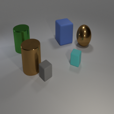
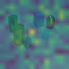
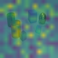
Figure 2: Gradient-based visualizations of an intermediate output (attention on the brown cylinder) of a neural module network produce unreliable attention masks. Furthermore, changing a downstream module from query color (middle) to query size (right) alters the visualization of the attention.

Attention. Some approaches [1, 4, 18, 26, 27, 28] propose an attention mechanism whereby each word corresponds to some feature of an image. One major difficulty with this type of approach is that some words have no clear semantic content in image-space. For example, the word ‘sitting’ does not have a clear region of focus in the question “What object is the man sitting on?”, and seems to rely on further analysis of the semantics of the question. The key components of this question are ‘man’ and ‘object being [sat] on.’ This is a problem for the natural language processing pipeline rather than the visual component of a system.

Several authors [7, 10, 25] have proposed attention mechanisms that a network can use, optionally. In the context of providing transparent models, this can be problematic as a network can learn not to use an attended region at all. By explicitly forcing the attention mechanism to be used, we ensure our network uses attended regions in an intuitive way.

Many authors [1, 4, 6, 12, 17, 18, 26, 27, 23, 28, 33] use a spatial softmax to compute attention weights. This enforces a global normalization across an image, which results in scene-dependent attention magnitudes. For example, in an image with a single car, a model asked to attend to the cars would ideally put zero attention on every region that does not contain a car and full (unity) attention on the region containing the car. In an image with two cars, a spatial softmax will force each car region to have an attention magnitude of one-half. This issue is noted by Zhang et al. [31] in the context of counting, but we note a more general problem. To addres this, we utilize an elementwise sigmoid to ensure that the activation at each pixel lies between zero and one, and do not introduce any form of global normalization. Further details on our network architecture and motivation are supplied in the following section.

3 Transparency by Design

Breaking a complex chain of reasoning into a series of smaller subproblems, each of which can be solved independently and composed, is a powerful and intuitive means for reasoning. This type of modular structure also permits inspection of the the network output at each step in the reasoning process, contingent on module designs that produce interpretable outputs. Motivated by this, we introduce a neural module network that explicitly models an attention mechanism in image space, which we call a Transparency by Design network (TbD-net), following the fact that transparency is a motivating factor in our design decisions. Meant to achieve performance at the level of the model from Johnson et al. [14] while providing transparency similar to Andreas et al. [2] and Hu et al. [10], our model incorporates design decisions from all three architectures. The program generator from Johnson et al. [14] allows for impressive flexibility and performs exceptionally well, so we reuse this component in our network. We thus use their set of primitive operations, listed in Table 1, but redesign each module according to its intended function. The resulting modules are similar in spirit to the approaches taken by Andreas et al. [2] and Hu et al. [10].

To motivate this design decision, consider that some modules need only focus on local features in an image, as in the case of an Attention module which focuses on distinct objects or properties. Other modules need global context in order to carry out their operation, as in the case of Relate modules, which must be capable of shifting attention across an entire image. We combine our prior knowledge about each module’s task with empirical experimentation, resulting in a set of novel module architectures optimized for each operation.

In the visual question answering task, most steps in the reasoning chain require localizing objects that have some distinguishing visible property (e.g. color, material, etc.). We ensure that each TbD module performing this type of filtering outputs a one-dimensional attention mask, which explicitly demarcates the relevant spatial regions. Thus, rather than refine high-dimensional feature maps throughout the network, a TbD-net passes only attention masks between its modules. By intentionally forcing this behavior, we produce a strikingly interpretable and intuitive model. This marks a step away from complex neural networks as black boxes. Figure 3 shows an example of how a TbD-net’s attention shifts appropriately throughout its reasoning chain as it solves a complex VQA problem, and that this process is easily interpretable via direct visualization of the attention masks it produces. Note that our modules’ use of attention is not a learnable option, as it is in the work of Hu et al. [10]. Rather, our modules must utilize the attention that is passed into them, and thus must produce precise attention maps. All the attention masks we display were generated using a perceptually-uniform color map [11].

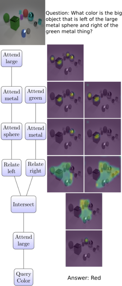
Figure 3: Read from top to bottom, a Transparency by Design network (TbD-net) composes visual attention masks to answer a question about objects in a scene. The tree diagram (left) indicates the modules used by the TbD-net, and their corresponding attention masks are depicted on the right.

3.1 Architecture Details

We now describe the architecture of each of our modules. Table 1 provides an overview of each module type. Several modules share input and output types (e.g. Attention and Relate) but differ in implementation, which is suited to their particular task. Additional details on the implementation and operation of each module can be found in the supplementary material.

Table 1: A summary of the modules used in our Transparency by Design network. ‘Attention’ and ‘Encoding’ refer to single- and high-dimensional outputs, respectively, from a preceding module. ‘Stem’ refers to image features produced by a trained neural network. The variables $x$ and $y$ refer to distinct objects in the scene, while [property] refers to one of color, shape, size, or material.

Module Type	Operation	Language Analogue
Attention	Attention $\times$ Stem $\rightarrow$ Attention	Which things are [property]?
Query	Attention $\times$ Stem $\rightarrow$ Encoding	What [property] is $x$?
Relate	Attention $\times$ Stem $\rightarrow$ Attention	Left of, right of, in front, behind
Same	Attention $\times$ Stem $\rightarrow$ Attention	Which things are the same [property] as $x$?
Comparison	Encoding $\times$ Encoding $\rightarrow$ Encoding	Are $x$ and $y$ the same [property]?
And	Attention $\times$ Attention $\rightarrow$ Attention	Left of $x$ and right of $y$
Or	Attention $\times$ Attention $\rightarrow$ Attention	Left of $x$ or right of $y$

We use image features extracted from ResNet-101 [8] and feed these through a simple convolutional block called the ‘stem,’ following the work of Johnson et al. [14]. Similar to Hu et al. [10], and a point of departure from Johnson et al. [14] and Andreas et al. [2], we provide stem features to most of our modules. This ensures image features are readily accessible to each module and no information is lost in long compositions. The stem translates high-dimensional feature input from ResNet into lower-dimensional features suitable for our task.

Attention modules attend to the regions of the image that contain an object with a specified property. For example, this type of module would be used to locate the red objects in a scene. The Attention module takes as input image features from the stem and a previous attention to refine (or an all-one tensor if it is the first Attention in the network) and outputs a heatmap of dimension $1\times H\times W$ corresponding to the objects of interest, which we refer to as an attention mask. This is done by multiplying the input image features by the input attention mask elementwise, then processing those attended features with a series of convolutions.

Logical And and Or modules combine two attention masks in a set intersection and union, respectively. These operations need not be learned, since they are already well-defined and can be implemented by hand. The And module takes the elementwise minimum of two attention masks, spatially, while the Or module takes the elementwise maximum.

A Relate module attends to a region that has some spatial relation to another region. For example, in the question “What color is the cube to the right of the small sphere?”, the network should determine the position of the small sphere using a series of Attention modules, then use a Relate module to attend to the region that is spatially to the right. This module needs global context in its operation, so that regions to the far right can be influenced by an object on the far left, for instance. Zhu et al. [32] aptly note that common VQA architectures have receptive fields that are too small for this global information propagation. They propose a structured solution using a conditional random field. Our solution is to use a series of dilated convolutions [29] in order to expand the receptive field to the entire image, providing the global context needed by Relate. These modules take as input image features from the stem and the attention mask from the previous module and output an attention mask.

A Same module attends to a region, extracts a relevant property from that region, and attends to every other region in the image that shares that property. As an example, when answering the question “Is anything the same color as the small cube?”, the network should localize the small cube via Attention modules, then use a Same module to determine its color and output an attention mask localizing all other objects sharing that color. As with the Relate module, a Same module must take into account context from distant spatial regions. However, the Same operation differs in its execution, since it must perform a more complex function. We perform a cross-correlation between the object of interest and every other object in the scene to determine which objects share the same property as the object of interest, then send this output through a convolutional layer to produce an attention mask. Hence, the Same modules take as input stem features and an attention mask and produce an attention mask.

Query modules extract a feature from an attended region of an image. For example, these modules would determine the color of an object of interest. Each Query takes as input stem features and an attention mask and produces a feature map encoding the relevant property. The image features are multiplied by the input attention elementwise, then processed by a series of convolutions. A Query module is also used for determining whether a given description matches any object (existence questions) and for counting.

A Compare module compares the properties output by two Query modules and produces a feature map which encodes whether the properties are the same. This module would be used to answer the question “Are the cube and the metal sphere the same size?”, for example. Two feature maps from Query modules are provided as input, concatenated, then processed by a series of convolutions. A feature map is output, encoding the relevant information.

The final piece of our module network is a classifier that takes as input the feature map from either a Query or Compare module and produces a distribution over answers. We again follow the work of Johnson et al. [14], using a series of convolutions, followed by max-pooling and fully-connected layers.

4 Experiments

We evaluate our model using the CLEVR dataset [13] and CLEVR-CoGenT. CLEVR is a VQA dataset consisting of a training set of 70k images and 700k questions, as well as test and validation sets of 15k images and 150k questions about objects in a rendered three-dimensional scene designed to test compositional reasoning. For more details about the task, we refer the reader to Johnson et al. [13].

In our model, all convolutional filters are initialized as described by He et al. [9]. Note that our architectural changes do not affect the natural language processing component from Johnson et al. [14], which determines the composition of a modular network. For simplicity, we use ground truth programs to train our network, because we do not modify the program generator. We find that training on ground truth programs does not affect the accuracy of the model from Johnson et al. [14], compared to training with generated programs. Our training procedure thus takes triplets $(x,z,a)$ of image, program, and answer for training. We use the Adam optimization method [15] with learning rate set to $10^{-4}$ and our module network is trained end-to-end with early stopping. The training procedures for CLEVR and for CoGenT are the same. Ground truth programs are not provided with the CLEVR and CoGenT test sets, so we use the program generator from Johnson et al. [14] to compute programs from questions. The testing procedure thus takes image and question pairs $(x,q)$, produces a program $\pi(q)$ to arrange modules, then produces an answer $\hat{a}=M_{\pi(q)}(x)$ where $M_{\pi(q)}$ is the arrangement of modules produced by the program generator.

4.1 CLEVR

Our initial model achieves 98.7% test accuracy on the CLEVR dataset, far outperforming other neural module network-based approaches. As we will describe, we utilize the attention masks produced by our model to refine this initial model, resulting in state-of-the-art performance of 99.1% accuracy. Given the large number of high-performing models on CLEVR [14, 24, 5, 19], we train our model 5 times for a statistical measure of performance, achieving mean validation accuracy of 99.1% with standard deviation 0.07. Further, we note that none of these other models are amenable to having their reasoning processes inspected in an intuitive way. As we will show, our model provides straightforward, interpretable outputs at every stage of the visual reasoning process.

4.1.1 Attention as a Diagnostic Tool

Regularization. Examining the attention masks produced by our initial model, we noticed noise in the background. While not detrimental to our model’s performance, these spurious regions of attention may be confusing to users attempting to garner an understanding of the model outputs. Our intuition behind this behavior is that the model is not penalized for producing small amounts of attention on background regions because the later Query modules are able to effectively ignore them, since they contain no objects. As a result, no error signal propagates back through the model to push these to zero. To address this, we apply weighted $L_{1}$ regularization to the intermediate attention mask outputs, providing an explicit signal to minimize unnecessary activations. Experimentally, we find a factor of $2.5\times 10^{-7}$ to be effective in reducing spurious attention while maintaining strong attentions in true regions of interest. A comparison of an Attention module output with and without this regularization can be seen in Figure 4. Without regularization, the module produces a small amount of attention on background regions, high attention on objects of interest, and zero attention on all other objects. When we add this regularization term, the spurious background activations fade, leaving a much more precise attention mask.

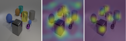
Figure 4: An input image (left) and the attention mask produced by the Attention[large] module overlaid atop the input image. Without penalizing attention mask outputs (middle) the attention mask is noisy and produces responses on background regions. Penalizing the attention outputs (right) provides a signal to reduce extraneous attention.

Spatial resolution. Examining the attention masks from our initial model indicated the resolution of the input feature maps is crucial for performance. Originally, our model took $14\times 14$ feature maps as input to each module. However, this was insufficient for resolving closely-spaced objects. Increasing the resolution of the input feature maps to $28\times 28$ alleviates these issues, which we do by extracting features from an earlier layer of ResNet. Figure 5 shows our model operating over $14\times 14$ and $28\times 28$ feature maps when asked to attend to an object in a narrow spatial region. Operating on $14\times 14$ feature maps, our model coarsely defines the region and incorrectly guesses that the object is a sphere. Using $28\times 28$ feature maps refines the region and allows the model to correctly identify the cylinder.

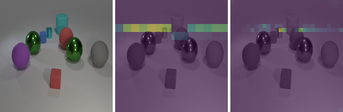
Figure 5: An input image (left) and the attention mask produced by the model when asked to attend to the region behind the blue rubber object and in front of the large cyan rubber cylinder with $14\times 14$ (middle) and $28\times 28$ (right) input features.

Performance improvements. By adding regularization and increasing spatial resolution, two strategies developed by examining our model attentions, we improve the accuracy of our model on CLEVR from 98.7% to 99.1%, a new state of the art. A full table of results including comparisons with several other approaches can be seen in Table 2. While conceptually similar to prior work in modular networks [2, 10, 14], our model differs drastically in module design. In addition to achieving superior performance, our paradigm allows for the verification of module behavior and informs network design.

Table 2: Performance comparison of state-of-the-art models on the CLEVR dataset. Our model performs well while maintaining model transparency. We achieve state of the art performance on Query questions, while remaining competitive in all other categories. Our TbD model is trained without regularizing the output attention masks, while ‘+ reg’ indicates the use of the regularization scheme described in the text. The ‘+ hres’ indicator shows a model was trained using higher-resolution $28\times 28$ feature maps rather than $14\times 14$ feature maps.

Model	Overall	Count	Compare	Exist	Query	Compare
			Numbers		Attribute	Attribute
NMN [2]	72.1	52.5	72.7	79.3	79.0	78.0
N2NMN [10]	88.8	68.5	84.9	85.7	90.0	88.8
Human [13]	92.6	86.7	86.4	96.6	95.0	96.0
CNN + LSTM + RN [21]	95.5	90.1	93.6	97.8	97.1	97.9
PG + EE (700k) [14]	96.9	92.7	98.7	97.1	98.1	98.9
CNN + GRU + FiLM [19]	97.6	94.5	93.8	99.2	99.2	99.0
DDRprog [24]	98.3	96.5	98.4	98.8	99.1	99.0
MAC [5]	98.9	97.2	99.4	99.5	99.3	99.5
TbD-net (Ours)	98.7	96.8	99.1	98.9	99.4	99.2
TbD + reg (Ours)	98.5	96.5	99.0	98.9	99.3	99.1
TbD + reg + hres (Ours)	99.1	97.6	99.4	99.2	99.5	99.6

4.1.2 Transparency

We examine the attention masks produced by the intermediate modules of our TbD model. We show that our model explicitly composes visual attention masks to arrive at an answer, leading to an unprecedented level of transparency in the neural network. Figure 3 shows the composition of visual attentions through an entire question. In this section, we provide a quantitative analysis of transparency. We further examine the outputs of several modules, displayed without any smoothing, showing that each step of any composition is straightforwardly interpretable.

Quantitative Analysis of Attention. Here we propose a quantitative analysis of the interpretability of visual attention, which will allow for direct comparison with subsequent work in this area. In this context, a module’s attention is interpretable if it visually highlights the correct objects in a scene, without ambiguity. Specifically, we measure how often the center-of-mass of an attended region overlaps with the appropriate regions of the ground truth segmentation. We perform this analysis for each of our Attention modules within a given chain of reasoning. The CLEVR dataset generator [13] was used to produce 1k images and 10k questions for evaluation. This analysis produces precision and recall metrics to summarize the interpretable quality of a model’s attention.

Our original TbD-net model has a recall of 0.86 and a precision of 0.41. This low precision is largely due to attention placed on the background (analyzing the performance on foreground objects alone yields a precision of 0.95). The modifications to our model detailed in Section 4.1.1 dramatically improve the interpretability metrics as evaluated on the full image (foreground and background). Adding regularization improves the recall and precision values to 0.92 and 0.90, respectively, and increasing the spatial resolution further improves the values to 0.99 and 0.98, respectively.

Qualitative Analysis of Attention. Figure 6 shows the output of an Attention module that focuses on metal objects. The output is sensible and matches our intuition of where attention should be placed in the image. Maximal attention is given to the metal objects and minimal attention to the rubber objects and to the background region.

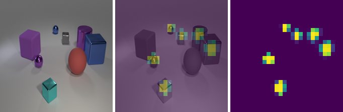
Figure 6: An input image (left) and the attention mask produced by the Attention[metal] module (right). When the attention mask is overlaid atop the input image (middle), it is apparent that the attention is appropriately focused on the metal objects.

The Attention modules are the simplest of the visual primitives. However, more complex operations, such as Same and Relate, still produce intuitive attention masks. We show in Figures 7 and 8 that these modules are just as transparent and easy to understand. The Relate module is given an attention mask highlighting the purple cylinder and shifts attention to the right. We see it highlights the entire region of the image, which it is able to do due to its expanded receptive field. The Same module is given an attention mask focusing on the blue sphere, then is asked to shift its focus to the objects of the same color. It gives maximal attention to the other three blue objects, minimal attention to all other objects, and a small amount of attention to the background.

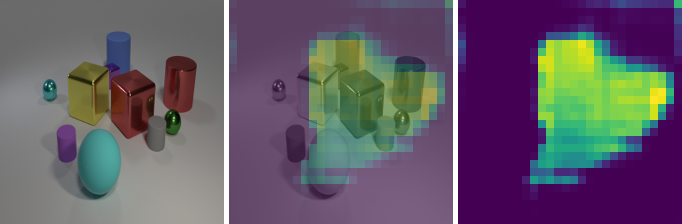
Figure 7: An input image (left) and the attention mask produced by the Relate[right] module (right) when it receives an attention on the purple cylinder. When the attention mask is overlaid atop the input image (middle), it is apparent that the attention is focused on the region to the right of the purple cylinder.

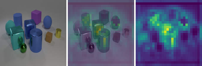
Figure 8: An input image (left) and the attention mask produced by the Same[color] module (right) when it receives an attention on the blue sphere. The attention mask overlaid atop the input image (middle) demonstrates that the module successfully performs the complex operation of (1) determining the color of the sphere (2) determining the color of all the other objects in the scene and (3) attending to the objects with the same color.

Our logical And and Or modules perform set intersection and union operations, respectively. Their behaviors are as intuitive as those set operations. Since Query and Compare modules output feature maps rather than attention masks, their outputs cannot be easily visualized. This is not problematic, as their corresponding operations do not have clear visual anchors. That is, it is not sensible to highlight image regions based on concepts such as ‘what shape’ or ‘are the same number,’ which have no referent without additional textual context.

4.2 CLEVR-CoGenT

The CLEVR-CoGenT dataset provides an excellent test for generalization. It is identical in form to the CLEVR dataset with the exception that it has two different conditions. In Condition A all cubes are colored one of gray, blue, brown, or yellow, and all cylinders are one of red, green, purple, or cyan; in Condition B the color palettes are swapped. This provides a check that the model does not tie together the notions of shape and color. In this section, we report only our best-performing model. Like previous work [14], our performance is worse on Condition B than Condition A after training only using Condition A data. As Table 3 shows, our model achieves 98.8% accuracy on Condition A, but only 75.4% on Condition B. Following Johnson et al. [14], we then fine-tune our model using 3k images and 30k questions from the Condition B data. Whereas other models see a significant drop in performance on the Condition A data after fine-tuning, our model maintains high performance. As Table 3 shows, our model can effectively learn from a small amount of Condition B data. We achieve 96.9% accuracy on Condition A and 96.3% accuracy on Condition B after fine-tuning, far surpassing the highest-reported 76.1% Condition A and 92.7% Condition B accuracy.

Table 3: Performance comparison against the current state-of-the-art model on the CoGenT dataset having trained only on Condition A data (middle column) and after fine-tuning on a small amount of data with novel attributes (right column).

	Train A		Fine-tune B
	A	B	A	B
PG + EE [14]	96.6	73.7	76.1	92.7
TbD + reg (Ours)	98.8	75.4	96.9	96.3

We perform an analysis of conditional probabilities based on shape/color dependencies to determine the cause of our model’s poor performance on Condition B before fine-tuning. Using the dataset from Section 4.1.2, we demonstrate that the model’s ability to identify shape, in particular, depends heavily on the co-occurrence of shape and color. Table 4 shows that the model is only able to effectively identify shapes in colors it has seen before fine-tuning, while it can identify color regardless of shape. Fine-tuning on Condition B rectifies the entanglement.

Table 4: Our model’s ability to determine the shape of an object depends heavily on the co-occurrence of shape and color before fine-tuning, while its ability to determine the color of an object does not. $P(\checkmark)$ indicates the probability of correctly identifying an object. $A$ and $B$ correspond to the CoGenT color/shape splits.

	Predict Shape		Predict Color
	$P(\checkmark|A)$	$P(\checkmark|B)$	$P(\checkmark|A)$	$P(\checkmark|B)$
Train A	0.90	0.22	0.91	0.84
Fine-tune B	0.77	0.81	0.90	0.86

Figure 9 shows this entanglement visually. When asked to attend to cubes before fine-tuning, our model correctly focuses on the gray and blue cubes in that image, but ignores the cyan cube and incorrectly places some attention on the brown cylinder. What is particularly noteworthy is the fact that our model’s representations of color are complete (with respect to CLEVR). When the network is asked to attend to the brown objects, it correctly identifies both the sphere and cylinder, even though it has only seen cubes and spheres in brown. Thus, our model has entangled its representation of shape with color, but has not entangled its representation of color with shape.

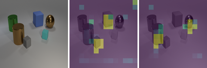
Figure 9: An input image (left) and the overlaid attention masks produced by Attention[cube] (middle) and Attention[brown] (right). Having never seen a cyan cube, Attention[cube] misses that object. Having never seen a brown cylinder, the model mistakenly places some attention on the brown cylinder in the scene. Conversely, Attention[brown] generalizes correctly, regardless of shape.

5 Discussion

We have presented Transparency by Design networks, which compose visual primitives that leverage an explicit attention mechanism to perform reasoning operations. Unlike their predecessors, the resulting neural module networks are both highly performant and readily interpretable. This is a key advantage to utilizing TbD models—the ability to directly evaluate the model’s learning process via the produced attention masks is a powerful diagnostic tool. One can leverage this capability to inspect the semantics of a visual operation, such as ‘same color,’ and redesign modules to address apparent aberrations in reasoning. Using these attentions as a means to improve performance, we achieve state-of-the-art accuracy on the challenging CLEVR dataset and the CoGenT generalization task. Such insight into a neural network’s operation may also help build user trust in visual reasoning systems.

Supplementary Material

6 Module Details

Here we describe each module in detail and provide motivation for specific architectural choices. In all descriptions, ‘image features’ refer to features that have been extracted using a pretrained model [8] and passed through our stem network, which is shared across modules. In all the following tables, $\delta(\cdot)$ will indicate a rectified linear function and $\sigma(\cdot)$ will indicate a sigmoid activation. The input size $R\times C$ indicates $R$ rows and $C$ columns in the input. In our original model, $R=C=14$, while our high-resolution model uses $R=C=28$.

The architecture of the Attention modules can be seen in Table 5. These modules take stem features and an attention mask as input and produce an attention mask as output. We first perform an elementwise multiplication of the input features and attention mask, broadcasting the attention mask along the channel dimension of the input features. We refer to this process as ‘attending to’ the features. We then process the attended features with two 3x3 convolutions, each with 128 filters and a ReLU, then use a single 1x1 convolution followed by a sigmoid to project down to an attention mask. This architecture is motivated by the design of the unary module from Johnson et al. [14].

Table 5: Architecture of an Attention module, which takes as input Features and an Attention and produces an Attention.

Index	Layer	Output Size
(1)	Features	$128\times R\times C$
(2)	Previous module output	$1\times R\times C$
(3)	Elementwise multiply (1) and (2)	$128\times R\times C$
(4)	$\delta$(Conv($3\times 3,128\rightarrow 128$))	$128\times R\times C$
(5)	$\delta$(Conv($3\times 3,128\rightarrow 128$))	$128\times R\times C$
(6)	$\sigma$(Conv($1\times 1,128\rightarrow 1$))	$1\times R\times C$

The And and Or modules, seen in Table 6 and Table 7, respectively, perform set intersection and union operations. These modules return the elementwise minimum and maximum, respectively, of two input attention masks. This is motivated by the logical operations that Hu et al. [10] implement, which seems a natural expression of these operations. Such simple and straightforward operations need not be learned, since they can be effectively and efficiently implemented by hand.

Table 6: Architecture of an And module. This module receives as input two Attentions and produces an Attention.

Index	Layer	Output Size
(1)	Previous module output	$1\times R\times C$
(2)	Previous module output	$1\times R\times C$
(3)	Elementwise minimum (1) and (2)	$1\times R\times C$

Table 7: Architecture of an Or module. This module receives as input two Attentions and produces an Attention.

Index	Layer	Output Size
(1)	Previous module output	$1\times R\times C$
(2)	Previous module output	$1\times R\times C$
(3)	Elementwise maximum (1) and (2)	$1\times R\times C$

The Relate module, shown in Table 8, needs global context to shift attention across an entire image. Motivated by this, we use a series of dilated 3x3 convolutions, with dilation factors 1, 2, 4, 8, and 1, to expand the receptive field to the entire image. The choice of dilation factors is informed by the work of Yu and Koltun [29]. These modules receive stem features and an attention mask and produce an attention mask. Each convolution in the series has 128 filters and is followed by a ReLU. A final convolution then reduces the feature map to a single-channel attention mask, and a sigmoid nonlinearity is applied.

Table 8: Architecture of a Relate module. These modules receive as input Features and an Attention and produce an Attention.

Index	Layer	Output Size
(1)	Features	$128\times R\times C$
(2)	Previous module output	$1\times R\times C$
(3)	Elementwise multiply (1) and (2)	$128\times R\times C$
(4)	$\delta$(Conv($3\times 3,128\rightarrow 128$, dilate 1))	$128\times R\times C$
(5)	$\delta$(Conv($3\times 3,128\rightarrow 128$, dilate 2))	$128\times R\times C$
(6)	$\delta$(Conv($3\times 3,128\rightarrow 128$, dilate 4))	$128\times R\times C$
(7)	$\delta$(Conv($3\times 3,128\rightarrow 128$, dilate 8))	$128\times R\times C$
(8)	$\delta$(Conv($3\times 3,128\rightarrow 128$, dilate 1))	$128\times R\times C$
(9)	$\sigma$(Conv($1\times 1,128\rightarrow 1$))	$1\times R\times C$

The Same module is the most complex of our modules, and the most complex operation we perform. To illustrate this, consider the Same[shape] module. It must determine the shape of the attended object, compare that shape with the shape of every other object in the scene (which requires global information propagation), and attend to all the objects that share that shape. Initially, we used a design similar to the Relate module to perform this operation, but found it did not perform well. After further reflection, we posited this was because the Relate module does not have a mechanism for remembering which object we are interested in performing the Same with respect to. Table 9 provides an overview of the Same module. Here we explicate the notation. Provided with stem features and an attention mask as input, we take the $\arg\max$ of the feature map, spatially. This gives us the $(x,y)$ position of the object of interest (i.e. the object to perform the Same with respect to). We then extract the feature vector at this spatial location in the input feature map, which gives us the vector encoding the property of interest (among other properties). Next, we perform an elementwise multiplication with the feature vector at every spatial dimension. This essentially performs a cross-correlation of the feature vector of interest with the feature vector of every other position in the image. Our intuition is that the vector dimensions that encode the property of interest will be ‘hot’ at every point sharing that property with the object of interest. At this point, a convolution could be learned that attends to the relevant regions. However, the Same operation, by its definition in CLEVR, must not attend to the original object. That is, an object is by definition not the same property as itself. Therefore, the Same module must learn not to attend to the original object. We thus concatenate the original input attention mask with the cross-correlated feature map, allowing the convolutional filter to know which object was the original, and thus ignore it.

Table 9: Architecture of a Same module. These modules receive as input Features and an Attention and produce an Attention.

Index	Layer	Output Size
(1)	Features	$128\times R\times C$
(2)	Previous module output	$1\times R\times C$
(3)	$\arg\max_{x,y}(2)$	$1\times 1\times 1$
(4)	$(1)_{(3)}$	$128\times 1\times 1$
(5)	Elementwise multiply (1) and (4)	$128\times R\times C$
(6)	Concatenate (5) and (2)	$129\times R\times C$
(7)	$\sigma$(Conv($1\times 1,129\rightarrow 1$))	$1\times R\times C$

The Query module architecture can be seen in Table 10. Its design is similar to that of the Attention modules and is likewise inspired by the unary module design of Johnson et al. [14] and adapted for receiving an attention mask and stem features as input. These modules produce a feature map as output, and thus do not have a convolutional filter that performs a down-projection.

Table 10: Architecture of a Query module. These modules receive as input Features and an Attention and produce an Encoding.

Index	Layer	Output Size
(1)	Features	$128\times R\times C$
(2)	Previous module output	$1\times R\times C$
(3)	Elementwise multiply (1) and (2)	$128\times R\times C$
(4)	$\delta$(Conv($3\times 3,128\rightarrow 128$))	$128\times R\times C$
(5)	$\delta$(Conv($3\times 3,128\rightarrow 128$))	$128\times R\times C$

The Compare module, shown in Table 11, is inspired by the binary module of Johnson et al. [14]. These modules take two feature maps as input and produce a feature map as output. Their purpose is to determine whether the two input feature maps encode the same property.

Table 11: Architecture of a Compare module. These modules receive as input two Features and produce an Encoding.

Index	Layer	Output Size
(1)	Previous module output	$128\times R\times C$
(2)	Previous module output	$128\times R\times C$
(3)	Concatenate (1) and (2)	$128\times R\times C$
(4)	$\delta$(Conv($1\times 1,128\rightarrow 128$))	$128\times R\times C$
(5)	$\delta$(Conv($3\times 3,128\rightarrow 128$))	$128\times R\times C$
(6)	$\delta$(Conv($3\times 3,128\rightarrow 128$))	$128\times R\times C$

References

- [1] P. Anderson, X. He, C. Buehler, D. Teney, M. Johnson, S. Gould, and L. Zhang. Bottom-Up and Top-Down Attention for Image Captioning and VQA. ArXiv e-prints, July 2017.
- [2] J. Andreas, M. Rohrbach, T. Darrell, and D. Klein. Deep compositional question answering with neural module networks. CoRR, abs/1511.02799, 2015.
- [3] J. Andreas, M. Rohrbach, T. Darrell, and D. Klein. Learning to compose neural networks for question answering. CoRR, abs/1601.01705, 2016.
- [4] K. Chen, J. Wang, L. Chen, H. Gao, W. Xu, and R. Nevatia. ABC-CNN: an attention based convolutional neural network for visual question answering. CoRR, abs/1511.05960, 2015.
- [5] C. D. M. Drew Arad Hudson. Compositional attention networks for machine reasoning. International Conference on Learning Representations, 2018. accepted as poster.
- [6] A. Fukui, D. Huk Park, D. Yang, A. Rohrbach, T. Darrell, and M. Rohrbach. Multimodal Compact Bilinear Pooling for Visual Question Answering and Visual Grounding. ArXiv e-prints, June 2016.
- [7] A. W. Harley, K. G. Derpanis, and I. Kokkinos. Segmentation-aware convolutional networks using local attention masks. CoRR, abs/1708.04607, 2017.
- [8] K. He, X. Zhang, S. Ren, and J. Sun. Deep residual learning for image recognition. CoRR, abs/1512.03385, 2015.
- [9] K. He, X. Zhang, S. Ren, and J. Sun. Delving deep into rectifiers: Surpassing human-level performance on imagenet classification. CoRR, abs/1502.01852, 2015.
- [10] R. Hu, J. Andreas, M. Rohrbach, T. Darrell, and K. Saenko. Learning to reason: End-to-end module networks for visual question answering. CoRR, abs/1704.05526, 2017.
- [11] J. D. Hunter. Matplotlib: A 2d graphics environment. Computing In Science & Engineering, 9(3):90–95, 2007.
- [12] Z. Ji, K. Xiong, Y. Pang, and X. Li. Video summarization with attention-based encoder-decoder networks. CoRR, abs/1708.09545, 2017.
- [13] J. Johnson, B. Hariharan, L. van der Maaten, L. Fei-Fei, C. L. Zitnick, and R. B. Girshick. CLEVR: A diagnostic dataset for compositional language and elementary visual reasoning. CoRR, abs/1612.06890, 2016.
- [14] J. Johnson, B. Hariharan, L. van der Maaten, J. Hoffman, L. Fei-Fei, C. L. Zitnick, and R. Girshick. Inferring and executing programs for visual reasoning. In ICCV, 2017.
- [15] D. P. Kingma and J. Ba. Adam: A method for stochastic optimization. CoRR, abs/1412.6980, 2014.
- [16] Z. C. Lipton. The Mythos of Model Interpretability. ArXiv e-prints, June 2016.
- [17] N. Liu and J. Han. Picanet: Learning pixel-wise contextual attention in convnets and its application in saliency detection. CoRR, abs/1708.06433, 2017.
- [18] J. Lu, J. Yang, D. Batra, and D. Parikh. Hierarchical Question-Image Co-Attention for Visual Question Answering. ArXiv e-prints, May 2016.
- [19] E. Perez, H. de Vries, F. Strub, V. Dumoulin, and A. Courville. Learning Visual Reasoning Without Strong Priors. ArXiv e-prints, July 2017.
- [20] A. Rahimpour, L. Liu, A. Taalimi, Y. Song, and H. Qi. Person Re-identification Using Visual Attention. ArXiv e-prints, July 2017.
- [21] A. Santoro, D. Raposo, D. G. T. Barrett, M. Malinowski, R. Pascanu, P. Battaglia, and T. Lillicrap. A simple neural network module for relational reasoning. ArXiv e-prints, June 2017.
- [22] R. R. Selvaraju, M. Cogswell, A. Das, R. Vedantam, D. Parikh, and D. Batra. Grad-CAM: Visual Explanations from Deep Networks via Gradient-based Localization. ArXiv e-prints, Oct. 2016.
- [23] K. J. Shih, S. Singh, and D. Hoiem. Where To Look: Focus Regions for Visual Question Answering. ArXiv e-prints, Nov. 2015.
- [24] J. Suarez, J. Johnson, and F.-F. Li. DDRprog: A CLEVR differentiable dynamic reasoning programmer, 2018.
- [25] F. Wang, M. Jiang, C. Qian, S. Yang, C. Li, H. Zhang, X. Wang, and X. Tang. Residual Attention Network for Image Classification. ArXiv e-prints, Apr. 2017.
- [26] H. Xu and K. Saenko. Ask, Attend and Answer: Exploring Question-Guided Spatial Attention for Visual Question Answering. ArXiv e-prints, Nov. 2015.
- [27] K. Xu, J. Ba, R. Kiros, K. Cho, A. C. Courville, R. Salakhutdinov, R. S. Zemel, and Y. Bengio. Show, attend and tell: Neural image caption generation with visual attention. CoRR, abs/1502.03044, 2015.
- [28] Z. Yang, X. He, J. Gao, L. Deng, and A. Smola. Stacked Attention Networks for Image Question Answering. ArXiv e-prints, Nov. 2015.
- [29] F. Yu and V. Koltun. Multi-scale context aggregation by dilated convolutions. In ICLR, 2016.
- [30] Z. Yu, J. Yu, J. Fan, and D. Tao. Multi-modal Factorized Bilinear Pooling with Co-Attention Learning for Visual Question Answering. ArXiv e-prints, Aug. 2017.
- [31] Y. Zhang, J. Hare, and A. Prügel-Bennett. Learning to count objects in natural images for visual question answering. In International Conference on Learning Representations, 2018.
- [32] C. Zhu, Y. Zhao, S. Huang, K. Tu, and Y. Ma. Structured Attentions for Visual Question Answering. ArXiv e-prints, Aug. 2017.
- [33] Y. Zhu, O. Groth, M. Bernstein, and L. Fei-Fei. Visual7W: Grounded Question Answering in Images. ArXiv e-prints, Nov. 2015.