Newton-type Alternating Minimization Algorithm for Convex Optimization

Abstract

We propose NAMA (Newton-type Alternating Minimization Algorithm) for solving structured nonsmooth convex optimization problems where the sum of two functions is to be minimized, one being strongly convex and the other composed with a linear mapping. The proposed algorithm is a line-search method over a continuous, real-valued, exact penalty function for the corresponding dual problem, which is computed by evaluating the augmented Lagrangian at the primal points obtained by alternating minimizations. As a consequence, NAMA relies on exactly the same computations as the classical alternating minimization algorithm (AMA), also known as the dual proximal gradient method. Under standard assumptions the proposed algorithm possesses strong convergence properties, while under mild additional assumptions the asymptotic convergence is superlinear, provided that the search directions are chosen according to quasi-Newton formulas. Due to its simplicity, the proposed method is well suited for embedded applications and large-scale problems. Experiments show that using limited-memory directions in NAMA greatly improves the convergence speed over AMA and its accelerated variant.

I Introduction

We consider convex optimization problems of the form

$$\operatorname*{minimize\ }_{x\in{{\rm I\mathchoice{}{}{}{}R}}^{n}}\ f(x)+g(Ax),$$

where $f$ is strongly convex, $g$ is convex and $A$ is a linear mapping. Problems of this form are quite general and appear in various areas of applications, including optimal control [1], system identification [2] and machine learning [3, 4]. For example, whenever $g$ is the indicator function of a convex set $C$, then (I) models a constrained convex problem: if $C$ is a box, then in particular (I) amounts to minimizing a strongly convex function subject to polyhedral constraints.

A general approach to the solution of (I) is based on the dual proximal gradient method, or forward-backward splitting, also known as alternating minimization algorithm (AMA) [5]. This is the dual application of an algorithm introduced by Lions and Mercier [6] for finding the zero of the sum of two maximal monotone operators, one of which is assumed to be co-coercive. The alternating minimization algorithm is intimately tied to the framework of augmented Lagrangian methods, and its global convergence and complexity bounds are well covered in the literature, see [5]: a global convergence rate of order $O(1/\sqrt{k})$ holds for the primal iterates of AMA under very general assumptions, and can be improved to the optimal rate $O(1/k)$ using a simple acceleration technique due to Nesterov, see [7, 8, 9].

As with all first order methods, the performance of (fast) AMA is severely affected by ill-conditioning of the problem [1]. One way to deal with this issue, which is extensively used in classical smooth, unconstrained optimization, is to precondition the problem using (approximate) second-order information on the cost function, as in (quasi-) Newton methods. However, both (I) and its dual are nonsmooth in general. This motivates considering the concept of alternating minimization envelope (AME): this is a real-valued (as opposed to extended real-valued) exact merit function for the dual problem, and is precisely the augmented Lagrangian associated with (I) evaluated at the primal points computed by AMA. Under mild assumptions on (I), the AME is continuously differentiable around the set of dual solutions and even strictly twice differentiable there. As a consequence, the AME allows to extend classical, smooth unconstrained optimization algorithms to the solution of the dual problem to (I), which is nonsmooth in general. In this work we propose a dual line-search method, which uses the AME as merit function to compute the stepsizes. The convergence properties of the proposed algorithm greatly improve over AMA when fast-converging directions, computed by means of quasi-Newton formulas, are followed. Furthermore, we show that the AME is equivalent to the forward-backward envelope (FBE, see [10, 11, 12]) associated with the dual problem.

I-A Related works

The FBE, as a tool for extending smooth unconstrained algorithms to nonsmooth problems, has first been introduced in [10]: there, two semismooth Newton methods are proposed for minimizing the sum of two convex functions, one of which is smooth and the other having an efficiently computable proximal mapping. This is the classical setting in which the proximal gradient method (and its accelerated variant) can be applied. In [11] the convexity assumption on the smooth term is relaxed, and the authors propose a line-search method with global sublinear rate (in the convex case) and asymptotic superlinear rate when quasi-Newton directions are used: the algorithm relies on descent directions over the FBE which is required to be everywhere differentiable. In [13] classical gradient-based line-search methods are considered for minimizing the FBE, see also [14]. In [12] the most general framework, where both summands are allowed to be nonconvex, is taken into account. In this case differentiability of the FBE cannot be assumed: a new algorithm is proposed which computes fast convergent directions with no need for gradient information on the FBE.

A similar approach was used in [15, 16] to accelerate other splitting algorithms, namely the Douglas-Rachford splitting and its dual counterpart ADMM.

I-B Contributions and organization of the paper

In the present paper we deal with the case where $g$ in (I) is composed with a linear mapping. In this case, even though $g$ may possess an efficiently computable proximal mapping, $g\circ A$ in general does not. This motivates addressing the dual problem of (I) instead. The contributions and organization of the present work can be summarized as follows.

• We propose the Newton-type Alternating Minimization Algorithm (NAMA, Section II, Algorithm 1), a generalization of the alternating minimization algorithm that performs a line-search step over the AME: the proposed algorithm relies on the very same alternating minimization operations of AMA.

• We show that the AME is equivalent to the FBE of the dual problem (Section III). This observation extends a classical result by Rockafellar, relating the Moreau envelope and the augmented Lagrangian, to our setting where an additional strongly convex term is present.

• We show that the proposed method enjoys global sublinear convergence under standard assumptions, and local linear convergence assuming calmness of the subdifferentials of the problem terms (Section IV).

• We analyze the first- and second-order properties of the AME, by linking them to generalized second-order properties of the primal functions $f$ and $g$ (Section V).

• We show that the proposed method converges asymptotically superlinearly when the dual problem has a (unique) strong dual minimum, and the line-search directions are selected so as to satisfy the Dennis-Moré condition, as it is the case when quasi-Newton update formulas are adopted (Section VI). The effectiveness of our approach is demonstrated by numerical simulations on linear MPC problems (Section VII).

Differently from the approaches in [11, 13, 14], NAMA does not require the gradient of the envelope function, therefore no second-order information on the smooth term is needed: this would severely limit its applicability in the present setting where the dual problem is solved. Furthermore, with respect to the approaches of [13, 14], the algorithm presented here possesses strong global convergence properties which are not typical of classical line-search methods. Differently from [12], despite the fact that the selected directions may not be descent directions and the line search is performed on the envelope function, NAMA is a descent method for the dual objective: this allows to simplify the convergence analysis of the method, and to show the global sublinear convergence rate for the dual cost and the primal iterates.

I-C Notation

In what follows $\langle{}\cdot{},{}\cdot{}\rangle$ denotes an inner product over a Euclidean space (whose nature will be clear from the context) and $\|\cdot\|=\sqrt{\langle{}\cdot{},{}\cdot{}\rangle}$ is the associated norm. For a linear $A:{{\rm I\mathchoice{}{}{}{}R}}^{n}\to{{\rm I\mathchoice{}{}{}{}R}}^{m}$, $\|A\|$ is the operator norm induced by the inner products over ${{\rm I\mathchoice{}{}{}{}R}}^{n}$ and ${{\rm I\mathchoice{}{}{}{}R}}^{m}$. For a set $C$, we denote by $\operatorname{ri}(C)$ its relative interior, and by $\operatorname{\Pi}_{C}(x)=\operatorname*{\arg\!\min}_{y\in C}\|y-x\|$ the projection onto $C$ in the considered norm. We denote the extended real line by $\overline{{\rm I\mathchoice{}{}{}{}R}}={{\rm I\mathchoice{}{}{}{}R}}\cup{\mathopen{}\left\{\infty{}\mid{}{}\right\}\mathclose{}}$, and by $\Gamma_{0}({{\rm I\mathchoice{}{}{}{}R}}^{n})$ the set of proper, closed, convex functions defined over ${{\rm I\mathchoice{}{}{}{}R}}^{n}$ with values in $\overline{{\rm I\mathchoice{}{}{}{}R}}$. For $h\in\Gamma_{0}({{\rm I\mathchoice{}{}{}{}R}}^{n})$ its Fenchel conjugate $h^{\ast}$, defined as $h^{\ast}(y)={\sup}_{x\in{{\rm I\mathchoice{}{}{}{}R}}^{n}}{\mathopen{}\left\{\langle{}x{},{}y{}\rangle-h(x){}\mid{}{}\right\}\mathclose{}}$ is also proper, closed and convex. Properties of conjugate functions are well described for example in [17, 18, 19, 20]. Among these we recall the Fenchel-Young inequality [19, Prop. 13.13]

$$\langle{}x{},{}y{}\rangle\leq h(x)+h^{\ast}(y)\quad\forall x,y,$$ (1)

with

$$y\in\partial h(x)\Leftrightarrow\langle{}x{},{}y{}\rangle=h(x)+h^{\ast}(y)\Leftrightarrow x\in\partial h^{\ast}(y),$$ (2)

see [17, Thm. 23.5]. For any $\gamma>0$, the proximal mapping associated with $h$, with stepsize $\gamma$, is denoted as

$$\operatorname{prox}_{\gamma h}(x)={\operatorname*{\arg\!\min}}_{z}{\mathopen{}\left\{h(z)+(\nicefrac{{1}}{{2\gamma}})\|z-x\|^{2}{}\mid{}{}\right\}\mathclose{}}.$$

This satisfies the Moreau identity [19, Thm. 14.3(ii)]

$$y=\operatorname{prox}_{\gamma h}(y)+\gamma\operatorname{prox}_{\gamma^{-1}h^{\ast}}(\gamma^{-1}y)\quad\forall y.$$ (3)

The value function of the problem defining $\operatorname{prox}_{\gamma h}$ is the Moreau envelope

$$h^{\gamma}(x)={\min}_{z}{\mathopen{}\left\{h(z)+(\nicefrac{{1}}{{2\gamma}})\|z-x\|^{2}{}\mid{}{}\right\}\mathclose{}}.$$

An alternative formulation for (I) is

$$\operatorname*{minimize\ }_{x\in{{\rm I\mathchoice{}{}{}{}R}}^{n},z\in{{\rm I\mathchoice{}{}{}{}R}}^{m}}f(x)+g(z)\quad\operatorname*{subject\ to\ }Ax=z.$$ (P^′)

Therefore we can define the augmented Lagrangian associated with (I), denoted as

$$\mathcal{L}_{\gamma}(x,z,y){}={}f(x)+g(z)+\langle{}y{},{}Ax-z{}\rangle+\tfrac{\gamma}{2}\|Ax-z\|^{2},$$

where $\gamma\geq 0$. We indicate by $\mathcal{L}\equiv\mathcal{L}_{0}$ the ordinary Lagrangian function.

We follow the terminology of [20] when referring to the concepts of strict continuity and strict differentiability. We say that a mapping $F:{{\rm I\mathchoice{}{}{}{}R}}^{n}\to{{\rm I\mathchoice{}{}{}{}R}}^{m}$ is strictly continuous at $\bar{x}$ if [20, Def. 9.1(b)]

$$\limsup_{\begin{subarray}{c}(x,y)\to(\bar{x},\bar{x})\\ x\neq y\end{subarray}}{\frac{\smash{\|F(y)-F(x)\|}}{\|y-x\|}}{}<{}\infty.$$

If $F$ is (Frechét) differentiable, we let $JF:{{\rm I\mathchoice{}{}{}{}R}}^{n}\to{{\rm I\mathchoice{}{}{}{}R}}^{m\times n}$ denote the Jacobian of $F$. When $m=1$ we indicate with $\nabla F=JF^{\top}$ the gradient of $F$ and with $\nabla^{2}F=J\nabla F^{\top}$ its Hessian, whenever it makes sense. We say that $F$ is strictly differentiable at $\bar{x}$ if it satisfies the stronger limit [20, Eq. 9(7)]

$$\lim_{\begin{subarray}{c}(x,y)\to(\bar{x},\bar{x})\\ x\neq y\end{subarray}}{\frac{\|F(y)-F(x)-JF({}\bar{x}{})[{}y-x{}]\|}{\|y-x\|}}{}={}0.$$

Some results in the paper are based on generalized second-order properties of extended-real-valued functions.

Definition I.1 ([20, Def. 13.6]).

Function $h:{{\rm I\mathchoice{}{}{}{}R}}^{n}\to\overline{{\rm I\mathchoice{}{}{}{}R}}$ is said to be twice epi-differentiable at $x$ for $v$, if the second-order difference quotient

$${\Delta}_{\tau}^{2}h{(}{x}{|}{v}{)}{[}{d}{]}{}={}\frac{\smash{h(x+\tau d)-h(x)-\tau\langle{}v{},{}d{}\rangle}}{\nicefrac{{\tau^{2}}}{{2}}}$$

epi-converges as $\tau\searrow 0$ (i.e., its epigraph converges in the sense of Painlevé-Kuratowksi, see [20, Def. 7.1]), the limit being the function ${\rm d}^{2}h{(}{x}{|}{v}{)}{[}{{}}{]}$ given by

$${\rm d}^{2}h{(}{x}{|}{v}{)}{[}{d}{]}=\liminf_{\begin{subarray}{c}\tau\searrow 0\\ d^{\prime}\to d\end{subarray}}{\Delta}_{\tau}^{2}h{(}{x}{|}{v}{)}{[}{d^{\prime}}{]}.$$

In this case ${\rm d}^{2}h{(}{x}{|}{v}{)}{[}{d}{]}$, as a function of $d$, is said to be the second-order epi-derivative of $h$ at $x$ for $v$. If ${\Delta}_{\tau}^{2}h{(}{\bar{x}}{|}{\bar{v}}{)}{[}{{}}{]}$ epi-converges as $\tau\searrow 0$, $\bar{x}\to x$ and $\bar{v}\to v$, then $h$ is said to be strictly twice epi-differentiable.

Twice epi-differentiability is a mild requirement, and functions with this property are abundant. Refer to [21, 22, 23, 24, 25] and to [20, §7, §13] for examples and an in-depth account on epi-derivatives, epi-differentiability, and their connections with ordinary differentiability.

II Background and proposed algorithm

Without further specifying it, throughout the paper we will work under the following basic assumption.

Assumption 1.

The following hold for (I):

1. (I) is feasible, i.e., $A\operatorname{dom}f\cap\operatorname{dom}g\neq\emptyset$;

2. $f\in\Gamma_{0}({{\rm I\mathchoice{}{}{}{}R}}^{n})$ is strongly convex with modulus $\mu_{f}>0$;

3. $g\in\Gamma_{0}({{\rm I\mathchoice{}{}{}{}R}}^{m})$.

Remark II.1.

Assumption 1 guarantees, by strong convexity of $f$, that a solution to (I) exists and is unique, be it $x_{\star}$. item 2) also implies that $f^{\ast}$ is Lipschitz continuously differentiable with constant $\mu_{f}^{-1}$ [20, Th. 12.60]. item 3) ensures that $g^{\ast}$ is also proper, closed, convex [19, Cor. 13.33], and its Moreau envelope $(g^{\ast})^{\gamma}$ is strictly continuous [20, Ex. 10.32] with $\gamma^{-1}$-Lipschitz gradient

$$\nabla(g^{\ast})^{\gamma}(y){}={}\gamma^{-1}{\mathopen{}\left(y-\operatorname{prox}_{\gamma g^{\ast}}(y)\right)\mathclose{}},$$ (4)

as shown in [19, Prop. 12.29]. ∎

The Fenchel dual problem associated with (I) is

$$\operatorname*{minimize\ }_{y\in{{\rm I\mathchoice{}{}{}{}R}}^{m}}\ \psi(y){}={}f^{\ast}(-A^{\top}y){}+{}g^{\ast}(y).$$

Under Assumption 1 strong duality holds, see [26, Thm. 5.2.1(b)-(c)] and primal-dual solutions $(x_{\star},y_{\star})$ to (I)-(II) are characterized by the first-order optimality conditions

$$-A^{\top}y_{\star}{}\in{}\partial f(x_{\star})\quad (\Leftrightarrow\ x_{\star}=\nabla f^{\ast}(-A^{\top}y_{\star}))$$ (4a)

$$y_{\star}{}\in{}\partial g(Ax_{\star})\quad (\Leftrightarrow\ Ax_{\star}\in\partial g^{\ast}(y_{\star})).$$ (4b)

A natural way to tackle (I) is to solve (II) by means of forward-backward splitting (or proximal gradient method): starting from an initial dual point $y^{0}\in{{\rm I\mathchoice{}{}{}{}R}}^{m}$, iterate

$$y^{k+1}=T_{\gamma}(y^{k})\coloneqq\operatorname{prox}_{\gamma g^{\ast}}(y^{k}+\gamma A\nabla f^{\ast}(-A^{\top}y^{k}))$$ (5)

for some positive stepsize parameter $\gamma$. If we define the associated fixed-point residual

$$R_{\gamma}(y){}\coloneqq{}\gamma^{-1}(y-T_{\gamma}(y)),$$

then dual optimality can be characterized as follows:

$$y_{\star}\in Y_{\star}\;\Leftrightarrow\;y_{\star}\in\operatorname*{fix}T_{\gamma}\;\Leftrightarrow\;y_{\star}\in\operatorname*{zer}R_{\gamma}\leavevmode\nobreak\ \leavevmode\nobreak\ \forall\gamma>0.$$ (6)

Iterations (5) are easily shown to be equivalent to the following scheme, the alternating minimization algorithm (AMA)

$$x^{k}{}={} \mathchoice{\hskip 12.06032pt\clap{\displaystyle x(y^{k})}\hskip 12.06032pt}{\hskip 12.06032pt\clap{x(y^{k})}\hskip 12.06032pt}{\hskip 8.485pt\clap{\scriptstyle x(y^{k})}\hskip 8.485pt}{\hskip 6.67203pt\clap{\scriptscriptstyle x(y^{k})}\hskip 6.67203pt}{}={}\operatorname*{\arg\!\min}_{x\in{{\rm I\mathchoice{}{}{}{}R}}^{n}}{\mathopen{}\left\{f(x)+\langle{}y^{k}{},{}Ax{}\rangle{}\mid{}{}\right\}\mathclose{}},$$ (7a)

$$z^{k}{}={} z_{\gamma}(y^{k}){}={}\operatorname*{\arg\!\min}_{z\in{{\rm I\mathchoice{}{}{}{}R}}^{m}}\mathcal{L}_{\gamma}(x^{k},z,y^{k}),$$ (7b)

$$y^{k+1}{}={} y^{k}+\gamma(Ax^{k}-z^{k}).$$ (7c)

Note that step (7b) can be equivalently formulated as

$$z^{k}=\operatorname{prox}_{\gamma^{-1}g}(\gamma^{-1}y^{k}+Ax(y^{k})).$$

Using the notation of (7), $T_{\gamma}$ and $R_{\gamma}$ can be expressed as

$$T_{\gamma}(y){}={} y+\gamma(Ax(y)-z_{\gamma}(y))$$ (8a)

$$R_{\gamma}(y){}={} z_{\gamma}(y)-Ax(y).$$ (8b)

It can be shown that $x^{k}\to x_{\star}$ in iterations (7), provided that $\gamma\in(0,\nicefrac{{2\mu_{f}}}{{\|A\|^{2}}})$, see [5, Prop. 3]. Moreover, the dual cost in this case converges sublinearly to the optimum with global rate $O(1/k)$, and the extrapolation techniques introduced by Nesterov [27, 28, 8] allow to obtain accelerated versions of AMA with an optimal global rate $O(1/k^{2})$, see [9]: we will here refer to this variant as fast AMA.

II-A Newton-type alternating minimization algorithm

Algorithm 1

Newton-type AMA (NAMA)

0:  Require            : $y^{0}\in{{\rm I\mathchoice{}{}{}{}R}}^{m}$, $\gamma\in(0,\nicefrac{{\mu_{f}}}{{\|A\|^{2}}})$, $\beta\in(0,1)$

0:  Initialize: $k=0$

1:  $x^{k}=\operatorname*{\arg\!\min}_{x}{\mathopen{}\left\{f(x)+\langle{}y^{k}{},{}Ax{}\rangle{}\mid{}{}\right\}\mathclose{}}$

1:  $\mathchoice{\hskip 8.80693pt\hbox to0.0pt{\hss$\displaystyle z^{k}$}}{\hskip 8.80693pt\hbox to0.0pt{\hss$z^{k}$}}{\hskip 6.20901pt\hbox to0.0pt{\hss$\scriptstyle z^{k}$}}{\hskip 5.06596pt\hbox to0.0pt{\hss$\scriptscriptstyle z^{k}$}}=\operatorname*{\arg\!\min}_{z}\mathcal{L}_{\gamma}(x^{k},z,y^{k})$

2:  Choose a direction $d^{k}\in{{\rm I\mathchoice{}{}{}{}R}}^{m}$

3:   Find the largest $\tau_{k}=\beta^{i_{k}},i_{k}\in{{\rm I\mathchoice{}{}{}{}N}},$ such that

$$\mathcal{L}_{\gamma}(\tilde{x}^{k},\tilde{z}^{k},\tilde{y}^{k})\geq\mathcal{L}_{\gamma}(x^{k},z^{k},y^{k}),$$ (9)

where

$$\tilde{y}^{k} {}={}y^{k}+\tau_{k}d^{k}+\gamma(1-\tau_{k})(Ax^{k}-z^{k})$$

$$\tilde{x}^{k} {}={}{\operatorname*{\arg\!\min}}_{x}{\mathopen{}\left\{f(x)+\langle{}\tilde{y}^{k}{},{}Ax{}\rangle{}\mid{}{}\right\}\mathclose{}}$$

$$\tilde{z}^{k} {}={}{\operatorname*{\arg\!\min}}_{z}\mathcal{L}_{\gamma}(\tilde{x}^{k},z,\tilde{y}^{k})$$

4:   $y^{k+1}=\tilde{y}^{k}+\gamma(A\tilde{x}^{k}-\tilde{z}^{k})$, $k=k+1$, go to step 1

The convergence speed of (fast) AMA is affected by ill-conditioning of the problem, as it is the case for all first-order methods. To accelerate convergence, we propose Algorithm 1. An overview of the algorithm is as follows:

• Algorithm 1 is composed by the very same operations as AMA: in fact, only alternating minimization steps with respect to $x$ and $z$ are performed.

• Step 3 computes a new dual iterate $\tilde{y}^{k}$, by performing a line-search over the augmented Lagrangian associated with (I) evaluated at the alternating minimization primal points: we will see that this is equivalent to the forward-backward envelope function associated with the dual problem (II).

• The line-search is performed using a convex combination of the “nominal” residual direction $\gamma(Ax^{k}-z^{k})$ and an “arbitrary” direction $d^{k}$, to be selected so as to ensure fast asymptotic convergence. This novel choice of direction ensures that the line-search is feasible at every iteration (i.e., condition (9) holds for a sufficiently small stepsize) despite the fact that $d^{k}$ may not be a direction of descent, as we will see.

• Step 4 will allow us to obtain global convergence rates, and it comes at no cost since vectors $\tilde{y}^{k},\tilde{x}^{k},\tilde{z}^{k}$ have already been computed in the line-search. In a sense, this step robustifies the algorithmic scheme.

By appropriately choosing $d^{k}$, the algorithm is able to greatly improve the convergence of AMA: we will prove that the algorithm converges with superlinear asymptotic rate when Newton-type directions are selected. For this reason we refer to Algorithm 1 as Newton-type Alternating Minimization Algorithm (NAMA).

Remark II.2 (AMA as special case).

If in Algorithm 1 one sets $d^{k}=0$ for all $k$, then one can trivially select $\tau_{k}=1$. In this case, $(\tilde{y}^{k},\tilde{x}^{k},\tilde{z}^{k}){}={}(y^{k},x^{k},z^{k})$ and Algorithm 1 reduces to AMA, cf. (7). ∎

Remark II.3 (General equality constrained problems).

For any proper, closed, convex $h:{{\rm I\mathchoice{}{}{}{}R}}^{r}\to\overline{{\rm I\mathchoice{}{}{}{}R}}$, $b\in{{\rm I\mathchoice{}{}{}{}R}}^{m}$ and linear mapping $B:{{\rm I\mathchoice{}{}{}{}R}}^{r}\rightarrow{{\rm I\mathchoice{}{}{}{}R}}^{m}$, a problem of the form

$$\operatorname*{minimize\ }_{x\in{{\rm I\mathchoice{}{}{}{}R}}^{n},w\in{{\rm I\mathchoice{}{}{}{}R}}^{r}}f(x)+h(w)\quad\operatorname*{subject\ to\ }Ax+Bw=b$$ (P^′′)

can be rewritten as (I) by letting

$$g(z)=(Bh)(b-z)=\inf_{w\in{{\rm I\mathchoice{}{}{}{}R}}^{r}}{\mathopen{}\left\{h(w){}\mid{}Bw=b-z\right\}\mathclose{}}.$$ (10)

Function $(Bh)$ is the image of $h$ under $B$, see [17, Thm. 5.7] and discussion thereafter. If we further assume $\operatorname{ri}(\operatorname{dom}h^{\ast})\cap\operatorname{range}(B^{\top})\neq\emptyset$, then $(Bh)$ is proper, closed, convex, see [17, Thm. 16.3], therefore $g$ in (10) satisfies item 3) (if $h$ is piecewise linear-quadratic then it is sufficient to assume $\operatorname{dom}h^{\ast}\cap\operatorname{range}(B^{\top})\neq\emptyset$, see [20, Cor. 11.33(b)]). In this case steps (7b) and (7c) of AMA become

$$w^{k}{}={} \operatorname*{\arg\!\min}_{w\in{{\rm I\mathchoice{}{}{}{}R}}^{r}}{\mathopen{}\left\{g(w)+\langle{}y^{k}{},{}Bw{}\rangle+\tfrac{\gamma}{2}\|Ax^{k}+Bw-b\|^{2}{}\mid{}{}\right\}\mathclose{}}$$

$$y^{k+1}{}={} y^{k}+\gamma(Ax^{k}+Bw^{k}-b).$$

Similar modifications allow to adapt NAMA to this more general setting: in light of these observations, what follows readily applies to problems of the form (P^′′). ∎

II-B Quasi-Newton directions

There is freedom in selecting $d^{k}$ in Algorithm 1. To accelerate the convergence of the iterates, one possible choice is to compute fast converging directions for the system of nonlinear equations $R_{\gamma}(y)=0$ characterizing dual optimal points, cf. (6). Specifically, in Algorithm 1 one can set

$$d^{k}=B_{k}^{-1}(Ax^{k}-z^{k}),$$ (11)

for a sequence of nonsingular matrices $(B_{k})_{k\in{{\rm I\mathchoice{}{}{}{}N}}}$ approximating in some sense the Jacobian $JR_{\gamma}$ at the limit point of the dual iterates $(y^{k})_{k\in{{\rm I\mathchoice{}{}{}{}N}}}$. In quasi-Newton methods, starting from an initial nonsingular matrix $B_{0}$, the sequence of matrices $(B_{k})_{k\in{{\rm I\mathchoice{}{}{}{}N}}}$ is determined by low-rank updates that satisfy the secant condition: in Algorithm 1 fast asymptotic convergence can be proved if

$$B_{k+1}p^{k}=q^{k}\quad\mbox{with}\quad{\mathopen{}\left\{\begin{array}[]{@{}l@{}l@{}}p^{k}{}={}&\tilde{y}^{k}-y^{k},\\ q^{k}{}={}&(\tilde{z}^{k}-A\tilde{x}^{k})-(z^{k}-Ax^{k}),\end{array}\right.\mathclose{}}$$

as will be discussed in Section VI. Note that all quantities required to compute the vectors $p^{k},q^{k}$ are available as by-product of the iterations.

In [29] the modified Broyden update is proposed, that prescribes rank-one updates of the form

$$\text{\it Broyden}\qquad B_{k+1}{}={}B_{k}{}+{}\theta_{k}\frac{(q^{k}-B_{k}p^{k})(p^{k})^{\top}}{\|p^{k}\|^{2}}.$$ (12)

Here, $(\theta_{k})_{k\in{{\rm I\mathchoice{}{}{}{}N}}}\subset[0,2]$ is a sequence used to ensure that all terms in $(B_{k})_{k\in{{\rm I\mathchoice{}{}{}{}N}}}$ are nonsingular, so that (11) is well defined. The original Broyden method [30] is obtained with $\theta_{k}\equiv 1$.

Probably the most popular quasi-Newton scheme is BFGS, which prescribes the following rank-two updates

$$\text{\it BFGS}\qquad B_{k+1}{}={}B_{k}+\frac{q^{k}(q^{k})^{\top}}{\langle{}q^{k}{},{}p^{k}{}\rangle}-\frac{B_{k}p^{k}(B_{k}p^{k})^{\top}}{\langle{}p^{k}{},{}B_{k}p^{k}{}\rangle}.$$ (13)

Note that in this case matrices $B_{k}$ are symmetric, and in fact the fast asymptotic properties of BFGS are guaranteed only if the Jacobian $JR_{\gamma}$ is symmetric [31] at the problem solution. This is not the case in our setting (cf. Example V.3) although we have observed that (13) often outperforms other non-symmetric updates such as (12) in practice.

Using the Sherman-Morrison-Woodbury identity in (12) and (13) allows to directly store and update $H_{k}=B_{k}^{-1}$, so that $d^{k}$ can be computed without inverting matrices or solving linear systems.

Ultimately, instead of storing and operating on dense $m\times m$ matrices, limited-memory variants of quasi-Newton schemes keep in memory only a few (usually $3$ to $30$) most recent pairs $(p^{k},q^{k})$ implicitly representing the approximate inverse Jacobian. Their employment considerably reduces storage and computations over the full-memory counterparts, and as such they are the methods of choice for large-scale problems. The most popular limited-memory method is probably L-BFGS, which is based on the update (13), but efficiently computes matrix-vector products with the approximate inverse Jacobian using a two-loop recursion procedure [32, 33, 34].

III Alternating minimization envelope

The fundamental tool enabling fast convergence of Algorithm 1 is the alternating minimization envelope function associated with (I). This is precisely the (negative) augmented Lagrangian function, evaluated at the primal points given by the alternating minimization steps.

Definition III.1 (Alternating minimization envelope).

The alternating minimization envelope (AME) for (I), with parameter $\gamma>0$, is the function

$$\psi_{\gamma}(y)=-\mathcal{L}_{\gamma}(x(y),z_{\gamma}(y),y).$$

The first observation that we make relates the alternating minimization envelope in Definition III.1 with the concept of forward-backward envelope.

Theorem III.2.

Function $\psi_{\gamma}$ is the forward-backward envelope (cf. [11, Def. 2.1]) associated with the dual problem (II):

$$\psi_{\gamma}(y) {}={}f^{\ast}(-A^{\top}y)+g^{\ast}(T_{\gamma}(y))+\tfrac{\gamma}{2}\|Ax(y)-z_{\gamma}(y)\|^{2}$$

$$\phantom{{}={}}+\gamma\langle{}Ax(y){},{}z_{\gamma}(y)-Ax(y){}\rangle.$$ (14)

Proof.

The optimality conditions for $x(y)$ and $z_{\gamma}(y)$ are

$$\partial f(x(y)) {}\ni{}-A^{\top}y,$$ (15a)

$$\partial g(z_{\gamma}(y)) {}\ni{}T_{\gamma}(y)=y+\gamma(Ax(y)-z_{\gamma}(y)).$$ (15b)

From these, using (2), we obtain

$$f(x(y))+f^{\ast}(-A^{\top}y) {}={}-\langle{}Ax(y){},{}y{}\rangle$$ (16a)

$$g(z_{\gamma}(y))+g^{\ast}(T_{\gamma}(y)) {}={}\langle{}z_{\gamma}(y){},{}T_{\gamma}(y){}\rangle$$ (16b)

Summing (16) and rearranging the terms we get (14). ∎

An alternative expression for $\psi_{\gamma}$ in terms of the Moreau envelope of $g^{\ast}$ is as follows, see [10]:

$$\psi_{\gamma}(y){}={}f^{\ast}(-A^{\top}y){}-{}\tfrac{\gamma}{2}\|Ax(y)\|^{2}{}+{}(g^{\ast})^{\gamma}(y+\gamma Ax(y)).$$ (17)

The AME enjoys several favorable properties, some of which we now summarize. For any $\gamma>0$, $\psi_{\gamma}$ is (strictly) continuous over ${{\rm I\mathchoice{}{}{}{}R}}^{m}$, whereas if $\gamma$ is small enough then the problem of minimizing $\psi_{\gamma}$ is equivalent to solving (II). These properties are listed in the next result.

Theorem III.3.

For any $\gamma>0$, $\psi_{\gamma}$ is a strictly continuous function on ${{\rm I\mathchoice{}{}{}{}R}}^{m}$ satisfying

1. $\psi_{\gamma}(y){}\leq{}\psi(y)+\tfrac{\gamma}{2}\|Ax(y)-z_{\gamma}(y)\|^{2}$,

2. $\psi_{\gamma}(y){}\geq{}\psi(T_{\gamma}(y)){}+{}\tfrac{\gamma}{2}{\mathopen{}\left(1-\tfrac{\gamma\|A\|^{2}}{\mu_{f}}\right)\mathclose{}}\|Ax(y)-z_{\gamma}(y)\|^{2}$,

for any $y\in{{\rm I\mathchoice{}{}{}{}R}}^{m}$. In particular, if $\gamma<\nicefrac{{\mu_{f}}}{{\|A\|^{2}}}$, then the following also holds

1. $\inf\psi_{\gamma}=\inf\psi$ and $\operatorname*{\arg\!\min}\psi_{\gamma}=\operatorname*{\arg\!\min}\psi$.

Proof.

Strict continuity of $\psi_{\gamma}$ follows immediately by the expression (17).

• 1): follows by Lem. .1 using $w=y$.

• 2): due to strong convexity of $f$, $f^{\ast}$ has $1/\mu_{f}$-Lipschitz gradient, and consequently

  $$f^{\ast}(-A^{\top}T_{\gamma}(y)) {}\leq{}f^{\ast}(-A^{\top}y)-\langle{}Ax(y){},{}T_{\gamma}(y)-y{}\rangle$$

  $$\phantom{{}\leq{}}+\tfrac{1}{2\mu_{f}}\|A^{\top}(T_{\gamma}(y)-y)\|^{2}$$

  $${}={}f^{\ast}(-A^{\top}y)-\gamma\langle{}Ax(y){},{}Ax(y)-z_{\gamma}(y){}\rangle$$

  $$\phantom{{}={}}+\tfrac{\gamma^{2}}{2\mu_{f}}\|A^{\top}(Ax(y)-z_{\gamma}(y))\|^{2}.$$ (18)

  Combining (14) with (18):

  $$\psi_{\gamma}(y) {}\geq{}\psi(T_{\gamma}(y))-\tfrac{\gamma^{2}}{2\mu_{f}}\|A^{\top}(Ax(y)-z_{\gamma}(y))\|^{2}$$

  $$\phantom{{}\leq{}}+\tfrac{\gamma}{2}\|Ax(y)-z_{\gamma}(y)\|^{2}$$

  $${}\geq{}\psi(T_{\gamma}(y))+\tfrac{\gamma}{2}{\mathopen{}\left(1-\tfrac{\gamma\|A\|^{2}}{\mu_{f}}\right)\mathclose{}}\|Ax(y)-z_{\gamma}(y)\|^{2}.$$

• 3): easily follows combining 1) and 2) with $y=y_{\star}\in Y_{\star}$, in light of the dual optimality condition (6). ∎

III-A Analogy with the dual Moreau envelope

Theorem III.2 highlights a clear connection between the augmented Lagrangian, the forward-backward envelope and the alternating minimization algorithm. This closely resembles the one, first noticed by Rockafellar [35, 36], relating the augmented Lagrangian, the Moreau envelope and the method of multipliers (also known as augmented Lagrangian method) by Hestenes and Powell [37, 38]. Consider the general linear equality constrained convex problem

$$\operatorname*{minimize\ }_{z\in{{\rm I\mathchoice{}{}{}{}R}}^{k}} g(z)$$ (19)

$$\operatorname*{subject\ to\ } Bz=b,$$

where $g:{{\rm I\mathchoice{}{}{}{}R}}^{m}\rightarrow\overline{{\rm I\mathchoice{}{}{}{}R}}$ is proper, closed, convex, $B\in{{\rm I\mathchoice{}{}{}{}R}}^{m\times k}$ and $b\in{{\rm I\mathchoice{}{}{}{}R}}^{m}$. When applied to the dual of (19), namely

$$\operatorname*{minimize\ }_{y\in{{\rm I\mathchoice{}{}{}{}R}}^{m}}\ \omega(y)=g^{\ast}(-B^{\top}y)+\langle{}b{},{}y{}\rangle,$$

the proximal minimization algorithm [39, §5.2] is equivalent to the following augmented Lagrangian method

$$z^{k}{}={} \operatorname*{\arg\!\min}_{z\in{{\rm I\mathchoice{}{}{}{}R}}^{n}}{\mathopen{}\left\{g(z)+\langle{}y^{k}{},{}Bz-b{}\rangle+\tfrac{\gamma}{2}\|Bz-b\|^{2}{}\mid{}{}\right\}\mathclose{}}$$

$$y^{k+1}{}={} y^{k}+\gamma(Bz^{k}-b).$$

If $\operatorname{range}(B^{\top})\cap\operatorname{ri}(\operatorname{dom}g^{\ast}){}\neq{}\emptyset$ one can show, with a similar proof to that of Theorem III.2, that the Moreau envelope of $\omega$ satisfies

$$\omega^{\gamma}(y^{k}){}={} -g(z^{k})-\langle{}y^{k}{},{}Bz^{k}-b{}\rangle-\tfrac{\gamma}{2}\|Bz^{k}-b\|^{2}$$

$${}={} -\mathcal{L}_{\gamma}(z^{k},y^{k}).$$

Therefore the forward-backward and Moreau envelope functions have the same nice interpretation in terms of augmented Lagrangian, when they are applied to the dual of equality constrained convex problems: in a sense, Theorem III.2 extends and generalizes the classical result on the dual Moreau envelope, by allowing for an additional variable $x$ and a strongly convex term $f$ in the problem.

IV Convergence

We now turn our attention to the global convergence properties of Algorithm 1. In light of Remark II.2, the results in this section directly apply to AMA, which is a special case of NAMA.

Remark IV.1 (Termination of line-search).

The line-search step 3 is well defined regardless of the choice of $d^{k}$: at any iteration $k$, condition (9) holds for $i_{k}$ sufficiently large. To see this, suppose that $\|Ax^{k}-z^{k}\|>0$ (otherwise $(x^{k},y^{k})$ is a primal-dual solution). Then, since $\gamma<\nicefrac{{\mu_{f}}}{{\|A\|^{2}}}$, Theorem III.3 implies that

$$\psi_{\gamma}(T_{\gamma}(y^{k}))<\psi_{\gamma}(y^{k}).$$ (20)

Since $\tilde{y}^{k}\to T_{\gamma}(y^{k})$ as $\tau_{k}\to 0$ and $\psi_{\gamma}$ is continuous, then necessarily $\psi_{\gamma}(\tilde{y}^{k})\leq\psi_{\gamma}(y^{k})$ for $\tau_{k}$ sufficiently small. ∎

Remark IV.2 (Bounded iteration complexity).

In the best case where $\tau_{k}=1$ is accepted in step 3, exactly two alternating minimizations are performed at iteration $k$. In practice, one can also impose a lower bound $\tau_{\min}>0$ for $\tau_{k}$: when $\tau_{k}<\tau_{\min}$ then the ordinary AMA update $y^{k+1}=y^{k}+\gamma(Ax^{k}-z^{k})$ is executed and the algorithm proceeds to the next iteration. This strategy results in a bounded iteration complexity for NAMA, and does not affect the convergence results of this and later sections. ∎

Theorem III.3 ensures that the following chain of inequalities, which will be fundamental for convergence results, holds in Algorithm 1:

$$\psi(y^{k+1}){}\leq{} \psi_{\gamma}(\tilde{y}^{k})$$ (21a)

$${}\leq{} \psi_{\gamma}(y^{k})$$ (21b)

$${}\leq{} \psi(y^{k})-\tfrac{\gamma}{2}\|Ax^{k}-z^{k}\|^{2}.$$ (21c)

In particular, Algorithm 1 is a descent method for $\psi$.

We now prove that the iterates of (1) converge to the dual optimal cost and to the primal solution. Moreover, global convergence rates are provided.

Theorem IV.3 (Global convergence).

In Algorithm 1:

1. $x^{k}\to x_{\star}$, $z^{k}\to Ax_{\star}$, and all cluster points of $(y^{k})_{k\in{{\rm I\mathchoice{}{}{}{}N}}}$ are dual optimal, i.e., they belong to $Y_{\star}$;

2. if $0\in\operatorname{int}(\operatorname{dom}g-A\operatorname{dom}f)$ then $\psi(y^{k})\searrow\inf\psi$ with global rate $O(1/k)$, and $x^{k}\to x_{\star}$ with global rate $O(1/\sqrt{k})$;

3. if $f$ and $g$ are piecewise linear-quadratic then $\psi(y^{k})\searrow\inf\psi$ with global Q-linear rate, and $x^{k}\to x_{\star}$ with global R-linear rate.

Proof.

• IV.3(i): by (21c), for all $i\geq 0$ we have

  $$\psi(y^{i+1})\leq\psi(y^{i})-\tfrac{\gamma}{2}\|Ax^{i}-z^{i}\|^{2}.$$

  By summing up the inequality for $i=1,\ldots,k$ we obtain

  $$\inf\psi\leq\psi(y^{k+1})\leq\psi(y^{1})-\frac{\gamma}{2}\sum_{i=1}^{k}\|Ax^{i}-z^{i}\|^{2}$$

  (the sum starts from $i=1$ since $y^{0}$ may be dual infeasible). In particular (cf. (8)) $R_{\gamma}(y^{k})=z^{k}-Ax^{k}\to 0$, and since $R_{\gamma}$ is continuous, necessarily all cluster points of $(y^{k})_{k\in{{\rm I\mathchoice{}{}{}{}N}}}$ are optimal. Moreover, it follows from Lem. .2 that the sequence $(x^{k})_{k\in{{\rm I\mathchoice{}{}{}{}N}}}$ is bounded. Let $K\subseteq{{\rm I\mathchoice{}{}{}{}N}}$ and $\bar{x}$ be such that $(x^{k})_{k\in K}\to\bar{x}$; then, since $Ax^{k}-z^{k}\to 0$ we also have that $(z^{k})_{k\in K}\to A\bar{x}$. By multiplying (15b) on the left by $A^{\top}$ and summing (15a) we obtain $\gamma A^{\top}(Ax_{k}-z_{k}){}\in{}\partial f(x_{k}){}+{}A^{\top}\partial g(z_{k})$. By letting $K\ni k\to\infty$, from outer semicontinuity of the subdifferential we obtain that

  $$0{}\in{}\partial f(\bar{x}){}+{}A^{\top}\partial g(A\bar{x}){}\subseteq{}\partial(f+g\circ A)(\bar{x})$$

  where the last inclusion follows from [17, Thm.s 23.8 and 23.9]. Thus, $\bar{x}$ is optimal, and being $x_{\star}$ the unique primal optimal (due to strong convexity), necessarily $\bar{x}=x_{\star}$. From the arbitrarity of the cluster point we conclude that $x^{k}\to x_{\star}$ and $z^{k}\to Ax_{\star}$.

• IV.3(ii): the assumed condition is equivalent to $Y_{\star}$ being nonempty and compact, see [26, Thm. 5.2.1], which implies that $\psi$ has bounded level sets [20, Prop. 3.23]. The proof proceeds similarly to that of [8, Thm. 4]. Let $D>0$ be such that $\operatorname{dist}(y,Y_{\star})<D$ for all points $y\in{\mathopen{}\left\{y\in{{\rm I\mathchoice{}{}{}{}R}}^{m}{}\mid{}\psi(y)\leq\psi(y^{0})\right\}\mathclose{}}$. From [11, Prop. 2.5] we know that $\psi_{\gamma}\leq\psi^{\gamma}$ (the Moreau envelope of $\psi$). Therefore,

  $$\psi(y^{k+1}){}\mathrel{{}\mathop{\leq}\limits^{\text{\clap{\eqref{eq:chain2}}}}}{}\psi_{\gamma}(y^{k}){}\leq{}\psi^{\gamma}(y^{k}){}={}\min_{\mathclap{w\in{{\rm I\mathchoice{}{}{}{}R}}^{m}}}{\mathopen{}\left\{\psi(w)+\tfrac{1}{2\gamma}\|w-y^{k}\|^{2}{}\mid{}{}\right\}\mathclose{}}$$

  and in particular, for $y_{\star}\in\operatorname*{\arg\!\min}\psi$,

  $$\psi(y^{k+1}){}\leq{} \min_{\alpha\in[0,1]}{{\mathopen{}\left\{\psi(\alpha y_{\star}+(1-\alpha)y^{k}){}+{}\tfrac{\alpha^{2}}{2\gamma}\|y^{k}-y_{\star}\|^{2}{}\mid{}{}\right\}\mathclose{}}}$$

  $${}\leq{} \min_{\alpha\in[0,1]}{{\mathopen{}\left\{\psi(y^{k})-\alpha(\psi(y^{k})-\inf\psi)+\tfrac{D^{2}}{2\gamma}\alpha^{2}{}\mid{}{}\right\}\mathclose{}}}$$

  where in last inequality we used convexity of $\psi$. In case $\psi(y^{0})-\inf\psi\geq D^{2}/\gamma$, then the optimal solution of the latter problem for $k=0$ is $\alpha=1$, and $\psi(y^{1})-\inf\psi{}\leq{}\nicefrac{{D^{2}}}{{2\gamma}}$. Otherwise, the optimal solution is

  $$\alpha{}={}\tfrac{\gamma}{D^{2}}(\psi(y^{k})-\inf\psi){}\leq{}\tfrac{\gamma}{D^{2}}(\psi(y^{0})-\inf\psi){}\leq{}1$$

  and we obtain

  $$\psi(y^{k+1}){}\leq{}\psi(y^{k}){}-{}\tfrac{\gamma}{2D^{2}}(\psi(y^{k})-\inf\psi)^{2}.$$

  By letting $\lambda_{k}=\frac{1}{\psi(y^{k})-\inf\psi}$ the last inequality becomes

  $$\lambda_{k+1}^{-1}\leq\lambda_{k}^{-1}-\tfrac{\gamma}{2D^{2}}\lambda_{k+1}^{-2}.$$

  By multiplying both sides by $\lambda_{k}\lambda_{k+1}$ and rearranging,

  $$\lambda_{k+1}\geq\lambda_{k}+\tfrac{\gamma}{2D^{2}}\tfrac{\lambda_{k+1}}{\lambda_{k}}\geq\lambda_{k}+\tfrac{\gamma}{2D^{2}},$$

  where the latter inequality follows from the fact that the sequence $(\psi(y^{k}))_{k\in{{\rm I\mathchoice{}{}{}{}N}}}$ is nonincreasing, as shown in (21). By telescoping the inequality we obtain

  $$\lambda_{k}{}\geq{}\lambda_{0}{}+{}k\tfrac{\gamma}{2D^{2}}{}\geq{}k\tfrac{\gamma}{2D^{2}},$$

  and therefore $\psi(y^{k})-\inf\psi{}\leq{}\nicefrac{{2D^{2}}}{{k\gamma}}$. This, together with Lem. .2, proves IV.3(ii).

• IV.3(iii): since the primal optimum is finite (see Rem. II.1), if $f$ and $g$ are piecewise linear-quadratic then $Y_{\star}$ is nonempty, see [20, Thm. 11.42, Ex. 11.43]. Using (21) we have that

  $$\psi(y^{k})-\psi(y^{k+1})\geq\tfrac{\gamma}{2}\|Ax^{k}-z^{k}\|^{2}.$$ (22)

  Furthermore, using Lem. .1 with $w=y_{\star}^{k}=\Pi_{Y_{\star}}y^{k}$ and $y=y^{k}$, we obtain

  $$\psi(y^{k+1})-\inf\psi {}\leq{}\psi_{\gamma}(y^{k})-\inf\psi$$

  $${}\leq{}\langle{}Ax^{k}-z^{k}{},{}y_{\star}^{k}-y^{k}{}\rangle-\tfrac{\gamma}{2}\|Ax^{k}-z^{k}\|^{2},$$

  where first inequality is due to (21c). This implies

  $$\psi(y^{k+1})-\inf\psi\leq\|Ax^{k}-z^{k}\|^{2}{\mathopen{}\left(\tfrac{\operatorname{dist}(y^{k},Y_{\star})}{\|Ax^{k}-z^{k}\|}-\tfrac{\gamma}{2}\right)\mathclose{}}$$

  which, by using (22), yields

  $$\psi(y^{k+1})-\inf\psi\leq{\mathopen{}\left(1-\tfrac{\gamma}{2}\tfrac{\|Ax^{k}-z^{k}\|}{\operatorname{dist}(y^{k},Y_{\star})}\right)\mathclose{}}(\psi(y^{k})-\inf\psi).$$ (23)

  It follows from [20, Thm. 11.14] that $f^{\ast}$ and $g^{\ast}$ are convex piecewise linear-quadratic in this case, and so is $\psi$. Therefore by [40, Thm. 2.7] $\psi$ enjoys the following quadratic growth condition: for any $\nu>0$ there is $\alpha>0$ such that

  $$\tfrac{\alpha}{2}\operatorname{dist}^{2}(y,Y_{\star})\leq\psi(y^{k})-\inf\psi\quad\forall y:\psi(y)-\inf\psi\leq\nu,$$

  which by [41, Cor. 3.6] is equivalent to the following error bound condition for some $\beta>0$

  $$\operatorname{dist}(y,Y_{\star})\leq\beta\|Ax(y)-z_{\gamma}(y)\|$$ (24)

  holding for all $y$ such that $\psi(y)-\inf\psi\leq\nu$. By using (24) in (23) we obtain global Q-linear convergence of $(\psi(y^{k}))_{k\in{{\rm I\mathchoice{}{}{}{}N}}}$, and from Lem. .2 global R-linear convergence of $(x^{k})_{k\in{{\rm I\mathchoice{}{}{}{}N}}}$ also follows. ∎

In general we can prove local linear convergence of Algorithm 1 provided that $\partial f$ and $\partial g$ are calm, according to the following definition (see [42, Sec. 3H, Ex. 3H.4]).

Definition IV.4 (Calmness of a mapping).

A multi-valued mapping $F:{{\rm I\mathchoice{}{}{}{}R}}^{m}\rightrightarrows{{\rm I\mathchoice{}{}{}{}R}}^{n}$ is said to be calm at $\bar{y}\in{{\rm I\mathchoice{}{}{}{}R}}^{m}$ for $\bar{x}\in F(\bar{y})$ if there is a neighborhood $U$ of $\bar{x}$ such that

$$F(y)\cap U\subseteq F(\bar{y})+O(\|y-\bar{y}\|),\quad\forall y\in{{\rm I\mathchoice{}{}{}{}R}}^{m}.$$

We simply say that $F$ is calm at $\bar{y}\in{{\rm I\mathchoice{}{}{}{}R}}^{m}$ (with no mention of $\bar{x}$) if it is calm at $\bar{y}\in{{\rm I\mathchoice{}{}{}{}R}}^{m}$ for all $\bar{x}\in F(\bar{y})$.

Calmness is a very common property of the subdifferential mapping. The subdifferential of all piecewise linear-quadratic functions is calm everywhere, as follows from [42, Prop. 3H.1]. Other examples include the nuclear and spectral norms [43]. Smooth functions, i.e., with Lipschitz gradient, clearly have calm subdifferential: this includes Moreau envelopes of closed, convex functions, such as the Huber loss for robust estimation, and commonly used loss functions such as the squared Euclidean norm and the logistic loss.

Calmness is equivalent to metric subregularity of the inverse mapping [42, Thm. 3H.3]: from [44, Prop. 6, Prop. 8] we then deduce that the indicator functions of $\ell_{1}$, $\ell_{\infty}$ and Euclidean norm balls all have calm subdifferentials.

The following result holds. Its proof is analogous to the one of [41, Thm. 4.2], although our assumption of calmness is equivalent to metric subregularity of $\partial f^{\ast}$ and $\partial g^{\ast}$, which is implied by the firm convexity assumed in [41].

Theorem IV.5 (Local linear convergence).

Suppose that the following hold for (I):

1. $0\in\operatorname{int}(\operatorname{dom}g-A\operatorname{dom}f)$ (nonempty, compact $Y_{\star}$);

2. $0\in\operatorname{ri}\partial(f+g\circ A)(x_{\star})$ (strict complementarity).

Suppose also that $\partial f$ is calm at $x_{\star}$ and $\partial g$ is calm at $Ax_{\star}$. Then in Algorithm 1 eventually $\psi(y^{k})\to\inf\psi$ with $Q$-linear rate and $x^{k}\to x_{\star}$ with $R$-linear rate.

Proof.

As discussed in the proof of IV.3(iii), it suffices to show that an error bound of the form (24) holds for some $\beta,\nu>0$.

The assumed calmness properties of $\partial f$ and $\partial g$ are equivalent to metric subregularity of $\partial f^{\ast}$ at $-A^{\top}y_{\star}$ for $x_{\star}$, and of $\partial g^{\ast}$ at $y_{\star}$ for $Ax_{\star}$, see [42, Thm. 3H.3], for all $y_{\star}\in Y_{\star}$. This can be seen, using [45, Thm. 3.3], to be equivalent to the following: there exist $c_{y_{\star}}>0$ and a neighborhood $U_{y_{\star}}$ of $y_{\star}$ such that for all $y\in U_{y_{\star}}$

$$f^{\ast}(-A^{\top}y){}\geq{} \phantom{{}+{}}f^{\ast}(-A^{\top}y_{\star})+\langle{}x_{\star}{},{}A^{\top}(y_{\star}-y){}\rangle$$

$${}+\tfrac{c_{y_{\star}}}{2}\operatorname{dist}^{2}(-A^{\top}y,(\nabla f^{\ast})^{-1}(x_{\star})),$$

$$g^{\ast}(y){}\geq{} \phantom{{}+{}}g^{\ast}(y_{\star})+\langle{}Ax_{\star}{},{}y-y_{\star}{}\rangle$$

$${}+\tfrac{c_{y_{\star}}}{2}\operatorname{dist}^{2}(y,(\partial g^{\ast})^{-1}(Ax_{\star})).$$

Since $Y_{\star}\subset\bigcup_{y_{\star}\in Y_{\star}}U_{y_{\star}}$ and $Y_{\star}$ is nonempty and compact (due to 1), see [26, Thm. 5.2.1]), we may select a finite subset $W\subset Y_{\star}$ such that $Y_{\star}\subset U_{Y_{\star}}=\bigcup_{y_{\star}\in W}U_{y_{\star}}$. Summing the above inequalities for all $y_{\star}\in W$, and denoting $c=\min{\mathopen{}\left\{c_{y_{\star}}{}\mid{}y_{\star}\in W\right\}\mathclose{}}>0$, we obtain

$$\psi(y){}\geq{}\inf\psi\\ {}+{}\tfrac{c}{2}{\mathopen{}\left[\operatorname{dist}^{2}(-A^{\top}y,\partial f(x_{\star}))+\operatorname{dist}^{2}(y,\partial g(Ax_{\star}))\right]\mathclose{}}$$ (25)

for all $y\in U_{Y_{\star}}$, where we have also used $(\nabla f^{\ast})^{-1}=\partial f$ and $(\partial g^{\ast})^{-1}=\partial g$. Note that 1) implies strict feasibility, therefore from Lem. .3, and the fact that for any $a,b\in{{\rm I\mathchoice{}{}{}{}R}}$, $a^{2}+b^{2}\geq 2ab$, we obtain that (25) implies

$$\psi(y)\geq\inf\psi+\tfrac{\kappa}{2}\operatorname{dist}^{2}(y,Y_{\star}),\quad\forall y\in U_{Y_{\star}},$$

for some $\kappa>0$, i.e., $\psi$ satisfies the quadratic growth condition, which by [41, Cor. 3.6] is equivalent to the error bound condition (24). This completes the proof. ∎

Remark IV.6 (Backtracking on $\gamma$).

In practice, no prior knowledge of the global Lipschitz constant $\nicefrac{{\|A\|^{2}}}{{\mu_{f}}}$ is required for Algorithm 1: instead of a fixed parameter $\gamma$, one can adaptively determine a sequence $(\gamma_{k})_{k\in{{\rm I\mathchoice{}{}{}{}N}}}$ essentially ensuring that inequalities (20) (which guarantees termination of the line-search step 3) and (21a) (which guarantees descent) hold at every iteration. This is done as follows. Select $\alpha\in(0,1)$ and initialize $\gamma_{0}>0$. At iteration $k$, let $\bar{y}^{k}=y^{k}+\gamma_{k}(Ax^{k}-z^{k})$ and $\bar{x}^{k}=x(\bar{y}^{k})$, and if

$$f(x^{k})>f(\bar{x}^{k})-\langle{}A^{\top}\bar{y}^{k}{},{}x^{k}-\bar{x}^{k}{}\rangle+\tfrac{\alpha\gamma}{2}\|Ax^{k}-z^{k}\|^{2},$$

then $\gamma_{k}\leftarrow\gamma_{k}/2$ and restart the iteration. Similarly if

$$f(\tilde{x}^{k})>f(x^{k+1})-\langle{}A^{\top}y^{k+1}{},{}\tilde{x}^{k}-x^{k+1}{}\rangle+\tfrac{\alpha\gamma}{2}\|A\tilde{x}^{k}-\tilde{z}^{k}\|^{2}.$$

As soon as $\gamma_{k}\leq\nicefrac{{\alpha\mu_{f}}}{{\|A\|^{2}}}$, the two inequalities above will never hold. As a consequence, $\gamma_{k}$ will be decreased only a finite number of times and will be constant starting from some iteration $\bar{k}$. The inequalities above are obtained by imposing the usual quadratic upper bound on $f^{\ast}\circ(-A^{\top})$, due to smoothness, and applying the conjugate subgradient theorem (2) in light of (15a). This procedure of adaptively adjusting $\gamma_{k}$ is analogous to what is done in practice in (fast) AMA, see [9, Rem. 3.4] and [7, §3, §4], and does not affect the validity of Thm.s IV.3 and IV.5. ∎

V First- and second-order properties

Algorithm 1 is a line-search method for the unconstrained minimization of $\psi_{\gamma}$ which, by Item 3), is equivalent to solving (II). To enable fast convergence of the iterates, we can apply ideas from smooth unconstrained optimization in selecting the sequence $(d^{k})_{k\in{{\rm I\mathchoice{}{}{}{}N}}}$ of directions. To this end, differentiability of $\psi_{\gamma}$ around dual solutions $y_{\star}$ is a desirable property. We will now see that this is implied by generalized second-order properties of $f$ around $x_{\star}$, which are introduced in the following assumption. Analogous assumptions on $g$ further ensure that $\psi_{\gamma}$ is (strictly) twice differentiable at $y_{\star}$. The interested reader is referred to [20] for an extensive discussion on (second-order) epi-differentiability.

Assumption 2.

The following hold with respect to a primal-dual solution $(x_{\star},y_{\star})$ to (I)-(II):

1. $f$ is strictly twice epi-differentiable at all $x\in\operatorname{dom}f$ close enough to $x_{\star}$, and in particular the second-order epi-derivative at $x_{\star}$ for $-A^{\top}y_{\star}$ is, for $w\in{{\rm I\mathchoice{}{}{}{}R}}^{n}$,

   $${\rm d}^{2}f{(}{x_{\star}}{|}{-A^{\top}y_{\star}}{)}{[}{w}{]}{}={}\langle{}H_{f}w{},{}w{}\rangle+\delta_{S_{f}}(w),$$ (26)

   where $S_{f}$ is a linear subspace of ${{\rm I\mathchoice{}{}{}{}R}}^{n}$ and $H_{f}\in{{\rm I\mathchoice{}{}{}{}R}}^{n\times n}$;

2. $g$ is (strictly) twice epi-differentiable at $Ax_{\star}$ for $y_{\star}$, with

   $${\rm d}^{2}g{(}{Ax_{\star}}{|}{y_{\star}}{)}{[}{w}{]}{}={}\langle{}H_{g}w{},{}w{}\rangle+\delta_{S_{g}}(w),$$ (27)

   for all $w\in{{\rm I\mathchoice{}{}{}{}R}}^{m}$, where $S_{g}$ is a linear subspace of ${{\rm I\mathchoice{}{}{}{}R}}^{m}$ and $H_{g}\in{{\rm I\mathchoice{}{}{}{}R}}^{m\times m}$.

When the stronger condition in parenthesis holds we will say that the assumptions are strictly satisfied.

Without loss of generality, we consider $H_{f}$ and $H_{g}$ symmetric and positive semidefinite, satisfying $\operatorname{range}(H_{f})=S_{f}$, $\operatorname{null}(H_{f})=S_{f}^{\bot}$, $\operatorname{range}(H_{g})\subseteq S_{g}$ and $\operatorname{null}(H_{g})\supseteq S_{g}^{\bot}$.

The requirements on $H_{f}$ and $H_{g}$ can indeed be made without loss of generality: matrix $H_{f}^{\prime}{}={}\frac{1}{2}\operatorname{\Pi}_{S_{f}}(H_{f}+H^{\top}_{f})\operatorname{\Pi}_{S_{f}}$ has the desired properties and satisfies (26) provided $H_{f}$ does, and similarly for $H_{g}$. In particular, it holds that

$$H_{f}{}={}\operatorname{\Pi}_{S_{f}}H_{f}\operatorname{\Pi}_{S_{f}}\quad\text{and}\quad H_{g}{}={}\operatorname{\Pi}_{S_{g}}H_{g}\operatorname{\Pi}_{S_{g}}.$$ (28)

Theorem V.1 (Differentiability of $\psi_{\gamma}$).

Suppose that Item 1) holds for a primal-dual solution $(x_{\star},y_{\star})$. Then $\psi_{\gamma}$ is of class $\mathcal{C}^{1}$ around $y_{\star}$, with

$$\nabla\psi_{\gamma}(y){}={}Q_{\gamma}(y)R_{\gamma}(y)$$

where $Q_{\gamma}(y)=I-\gamma A\nabla^{2}f^{\ast}(-A^{\top}y)A^{\top}$.

Proof.

From Lem. .4 it follows that ${\vphantom{f}\smash{\hat{f}}}=f^{\ast}\circ(-A^{\top})$ is of class $\mathcal{C}^{2}$ around $y_{\star}$. The claim now easily follows from the chain rule of differentiation applied to (17), by using (4). ∎

Twice differentiability of $\psi_{\gamma}$ at a dual solution $y_{\star}$ is very important: when Newton-type directions are used, this implies that eventually unit stepsize will be accepted and fast asymptotic convergence will take place. In other words, unlike standard nonsmooth merit functions for constrained optimization, $\psi_{\gamma}$ does not prevent the acceptance of unit stepsize.

Theorem V.2 (Twice differentiability of $\psi_{\gamma}$).

Suppose that Assumption 2 (strictly) holds with respect to a primal-dual solution $(x_{\star},y_{\star})$. Then,

1. $R_{\gamma}$ is (strictly) differentiable at $y_{\star}$ with Jacobian

   $$JR_{\gamma}({}y_{\star}{})[{}{}{}]=\gamma^{-1}{\mathopen{}\left[I-P_{\gamma}(y_{\star})Q_{\gamma}(y_{\star})\right]\mathclose{}};$$ (29)

   here, $Q_{\gamma}$ is as in Theorem V.1 and

   $$P_{\gamma}(y_{\star}){}={} J\operatorname{prox}_{\gamma g^{\ast}}{\mathopen{}\left(y_{\star}+\gamma A\nabla f^{\ast}(-A^{\top}y_{\star})\right)\mathclose{}}$$

   $${}={} \operatorname{\Pi}_{\bar{S}}{\mathopen{}\left(I+\gamma H_{g}^{\dagger}\right)\mathclose{}}^{-1}\operatorname{\Pi}_{\bar{S}}$$ (30)

   with $\bar{S}={S_{g}}^{\bot}+\operatorname{range}(H_{g})$;

2. $\psi_{\gamma}$ is (strictly) twice differentiable at $y_{\star}$ with symmetric Hessian

   $$\nabla^{2}\psi_{\gamma}(y_{\star}){}={}\gamma^{-1}Q_{\gamma}(y_{\star})\bigl{[}I-P_{\gamma}(y_{\star})Q_{\gamma}(y_{\star})\bigr{]}.$$ (31)

Proof.

Let ${\vphantom{f}\smash{\hat{f}}}=f^{\ast}\circ(-A^{\top})$ and $L_{\vphantom{f}\smash{\hat{f}}}=\nicefrac{{\mu_{f}}}{{\|A\|^{2}}}$. We know from [25, Thms. 3.8, 4.1] and [20, Thm. 13.21] that $\operatorname{prox}_{\gamma g^{\ast}}$ is (strictly) differentiable at $y_{\star}-\gamma{\nabla}\!{\vphantom{f}\smash{\hat{f}}}(y_{\star})$ if and only if $g$ (strictly) satisfies item 2); in fact, by (4) we know that $Ax_{\star}=-\nabla{\vphantom{f}\smash{\hat{f}}}(y_{\star})$. Moreover, due to Lem. .4, ${\vphantom{f}\smash{\hat{f}}}\in\mathcal{C}^{2}$ in a neighborhood of $y_{\star}$ and in particular $\nabla{\vphantom{f}\smash{\hat{f}}}$ is strictly differentiable at $y_{\star}$. The formula for $JR_{\gamma}({}y_{\star}{})[{}{}{}]$ follows from (4) and the chain rule of differentiation.

We now prove the claimed expression for $P_{\gamma}(y_{\star})$. We may invoke Lem. .5 and apply [20, Ex. 13.45] to the tilted function $g+\langle{}\nabla{\vphantom{f}\smash{\hat{f}}}(y_{\star}){},{}{}\cdot{}{}\rangle$ which this tells us that for all $d\in{{\rm I\mathchoice{}{}{}{}R}}^{m}$

$$P_{\gamma}(y_{\star})d$$

$$={} \operatorname{prox}_{(\gamma/2){\rm d}^{2}g^{\ast}{(}{y_{\star}}{|}{Ax_{\star}}{)}{[}{{}}{]}}(d)$$

$$={} \operatorname*{\arg\!\min}_{d^{\prime}\in\bar{S}}{{\mathopen{}\left\{\tfrac{1}{2}\langle{}d^{\prime}{},{}H_{g}^{\dagger}d^{\prime}{}\rangle+\tfrac{1}{2\gamma}\|d^{\prime}-d\|^{2}{}\mid{}{}\right\}\mathclose{}}}$$

$$={} \operatorname{\Pi}_{\bar{S}}\operatorname*{\arg\!\min}_{d^{\prime}\in{{\rm I\mathchoice{}{}{}{}R}}^{n}}{{\mathopen{}\left\{\tfrac{1}{2}\langle{}\operatorname{\Pi}_{\bar{S}}d^{\prime}{},{}\!\!H_{g}^{\dagger}\operatorname{\Pi}_{\bar{S}}d^{\prime}{}\rangle+\tfrac{1}{2\gamma}\|\operatorname{\Pi}_{\bar{S}}d^{\prime}-d\|^{2}{}\mid{}{}\right\}\mathclose{}}}$$

$$={} \operatorname{\Pi}_{\bar{S}}{\bigl{(}\operatorname{\Pi}_{\bar{S}}[I+\gamma H_{g}^{\dagger}]\operatorname{\Pi}_{\bar{S}}\bigr{)}}^{\dagger}\operatorname{\Pi}_{\bar{S}}d$$

where ^† indicates the pseudo-inverse. Observe now that, since $\operatorname{range}H_{g}^{\dagger}=\operatorname{range}H_{g}\subseteq\bar{S}$, we have

$$\operatorname{\Pi}_{\bar{S}}[I+\gamma H_{g}^{\dagger}]\operatorname{\Pi}_{\bar{S}}{}={}AB\quad\mbox{for}\quad A{}={}I+\gamma H_{g}^{\dagger}\leavevmode\nobreak\ \text{and}\leavevmode\nobreak\ B{}={}\operatorname{\Pi}_{\bar{S}}.$$

Moreover,

$$\operatorname{range}(A^{\top}AB){}\subseteq{} \operatorname{range}B,$$

$$\operatorname{range}(B^{\top}BA){}\subseteq{} {{\rm I\mathchoice{}{}{}{}R}}^{n}=\operatorname{range}(A),$$

therefore we can apply [46, Facts 6.4.12 (i)-(ii) and 6.1.6 (xxxii)] to see that ${\bigl{(}\operatorname{\Pi}_{\bar{S}}[I+\gamma H_{g}^{\dagger}]\operatorname{\Pi}_{\bar{S}}\bigr{)}}^{\dagger}{}={}\operatorname{\Pi}_{\bar{S}}[I+\gamma H_{g}^{\dagger}]^{-1}$, yielding (30).

Since $R_{\gamma}(y_{\star})=0$, from [11, Lem. 6.2] it follows that $\nabla\psi_{\gamma}=Q_{\gamma}R_{\gamma}$ is (strictly) differentiable at $y_{\star}$ provided that $Q_{\gamma}$ is (strictly) continuous at $y_{\star}$ and $R_{\gamma}$ is (strictly) differentiable at $y_{\star}$. A simple application of the chain rule of differentiation concludes the proof of 2). ∎

To better understand the requirements of Assumption 2, let us consider the following simple but significant example: when $f$ is $\mathcal{C}^{2}$ and $g\circ A$ models linear inequality constraints, Assumption 2 is implied by strict complementarity.

Example V.3 ($\mathcal{C}^{2}$ functions subject to polyhedral constraints).

Consider problems of the form

$$\operatorname*{minimize\ }_{x\in{{\rm I\mathchoice{}{}{}{}R}}^{n}}\ f(x)+\delta_{C}(Ax),$$

where $g=\delta_{C}$ is the indicator of $C={\mathopen{}\left\{z\in{{\rm I\mathchoice{}{}{}{}R}}^{m}{}\mid{}z\leq b\right\}\mathclose{}}$, $b\in{{\rm I\mathchoice{}{}{}{}R}}^{m}$, and $f\in\mathcal{C}^{2}$. In this case Item 1) holds with $H_{f}=\nabla^{2}f(x_{\star})$, $S_{f}={{\rm I\mathchoice{}{}{}{}R}}^{n}$ (therefore $\operatorname{\Pi}_{S_{f}}={\rm Id}$), see [20, Ex. 13.8]. Regarding Item 2), one can use [20, Ex. 13.17] to see that

$${\rm d}^{2}g{(}{Ax_{\star}}{|}{y_{\star}}{)}{[}{w}{]}{}={}\delta_{K(Ax_{\star},y_{\star})}(w),$$

where $K$ is the critical cone. Denoting as $T_{C}(y)$ the tangent cone of set $C$ at $y\in C$, and as $J={\mathopen{}\left\{i{}\mid{}(Ax_{\star})_{i}=b_{i}\right\}\mathclose{}}$ the set of active constraints at the solution $x_{\star}$, the critical cone is given by

$$K(Ax_{\star},y_{\star}) {}={}{\mathopen{}\left\{w\in T_{C}(Ax_{\star}){}\mid{}\langle{}y_{\star}{},{}w{}\rangle=0\right\}\mathclose{}}$$

$${}={}{\mathopen{}\left\{w{}\mid{}\langle{}y_{\star}{},{}w{}\rangle=0,w_{i}\leq 0\;\forall i\in J\right\}\mathclose{}}.$$

For $K(Ax_{\star},y_{\star})$ to be a subspace, necessarily $(y_{\star})_{i}>0$ for all $i\in J$, i.e., strict complementarity must hold at the primal-dual solution $(x_{\star},y_{\star})$. In this case, Item 2) holds with $H_{g}=0$ and

$$S_{g}=K(Ax_{\star},y_{\star})={\mathopen{}\left\{w{}\mid{}w_{i}=0\;\forall i\in J\right\}\mathclose{}}.$$

We may assume that $J={\mathopen{}\left\{1,\ldots,k{}\mid{}{}\right\}\mathclose{}}$ without loss of generality, i.e., the first $k$ constraints are the active ones, and let $\bar{J}={\mathopen{}\left\{1,\ldots,m{}\mid{}{}\right\}\mathclose{}}\setminus J$. Note that $\nabla^{2}f^{\ast}(-A^{\top}y_{\star})=\nabla^{2}f(x_{\star})^{-1}$ due to strong convexity of $f$, see [20, Ex. 11.9]. By partitioning the inverse Hessian and constraint matrix as

$$\nabla^{2}f(x_{\star})^{-1}=\begin{bmatrix}H_{JJ}&\quad H_{J\bar{J}}\\ H_{\bar{J}J}&\quad H_{\bar{J}\bar{J}}\\ \end{bmatrix},\quad A=\begin{bmatrix}A_{J}\\ A_{\bar{J}}\end{bmatrix},$$

and using the notation of Item 1) we obtain

$$P_{\gamma}(y_{\star})=\begin{bmatrix}I_{k}&0\\ 0&0\end{bmatrix},\quad JR_{\gamma}({}y_{\star}{})[{}{}{}]=\begin{bmatrix}A_{J}H_{J\!J}A_{J}^{\top}&A_{J}H_{J\!\bar{J}}A_{\bar{J}}^{\top}\\ 0&\tfrac{1}{\gamma}I_{m-k}\end{bmatrix},$$

as it follows by elementary computations. ∎

Finally, we can relate strong minimality of $\psi$ and $\psi_{\gamma}$ to nonsingularity of the Jacobian of $R_{\gamma}$ and to the generalized second-order properties of $f$ and $g$ as follows.

Theorem V.4 (Conditions for strong minimality).

If Assumption 2 holds for a primal-dual solution $(x_{\star},y_{\star})$, then for all $\gamma<\mu_{f}/\|A\|^{2}$ the following are equivalent:

1. $y_{\star}$ is a strong minimum for $\psi$;

2. $\nabla^{2}\psi_{\gamma}(y_{\star})$ is nonsingular (in fact, positive definite);

3. $JR_{\gamma}({}y_{\star}{})[{}{}{}]$ is nonsingular (in fact, similar to a symmetric and positive definite matrix);

4. $y_{\star}$ is a strong minimum for $\psi_{\gamma}$.

Proof.

•  V.4(b)  $\mathchoice{\hskip 5.0pt\clap{\displaystyle\Leftrightarrow}\hskip 5.0pt}{\hskip 5.0pt\clap{\Leftrightarrow}\hskip 5.0pt}{\hskip 3.5pt\clap{\scriptstyle\Leftrightarrow}\hskip 3.5pt}{\hskip 2.5pt\clap{\scriptscriptstyle\Leftrightarrow}\hskip 2.5pt}$  V.4(c) : Let $P=P_{\gamma}(y_{\star})$ and $Q=Q_{\gamma}(y_{\star})$ for brevity. Notice first that, due to item 3), $y_{\star}$ minimizes $\psi_{\gamma}$ and therefore $\nabla^{2}\psi_{\gamma}(y_{\star})\succeq 0$. Moreover, since $Q$ is symmetric and positive definite,

  $$JR_{\gamma}({}y_{\star}{})[{}{}{}]{}={}\gamma^{-1}(I-PQ){}\sim{}Q^{-\nicefrac{{1}}{{2}}}\nabla^{2}\psi_{\gamma}(y_{\star})Q^{-\nicefrac{{1}}{{2}}}$$

  the latter matrix being symmetric and positive semidefinite, where $\sim$ denotes the similitude relation.

•  V.4(b)  $\mathchoice{\hskip 5.0pt\clap{\displaystyle\Leftrightarrow}\hskip 5.0pt}{\hskip 5.0pt\clap{\Leftrightarrow}\hskip 5.0pt}{\hskip 3.5pt\clap{\scriptstyle\Leftrightarrow}\hskip 3.5pt}{\hskip 2.5pt\clap{\scriptscriptstyle\Leftrightarrow}\hskip 2.5pt}$  V.4(d) : trivial since $\nabla^{2}\psi_{\gamma}(y_{\star})$ exists.

•  V.4(d)  $\mathchoice{\hskip 5.0pt\clap{\displaystyle\Leftrightarrow}\hskip 5.0pt}{\hskip 5.0pt\clap{\Leftrightarrow}\hskip 5.0pt}{\hskip 3.5pt\clap{\scriptstyle\Leftrightarrow}\hskip 3.5pt}{\hskip 2.5pt\clap{\scriptscriptstyle\Leftrightarrow}\hskip 2.5pt}$  V.4(a) : the right implication is trivial since $\psi_{\gamma}\leq\psi$ and $\psi_{\gamma}(y_{\star})=\psi(y_{\star})$ as it follows from Thm. III.3. Suppose now that there exist $c,\varepsilon>0$ such that $\psi(y)-\psi(y_{\star}){}\geq{}\tfrac{c}{2}\|y-y_{\star}\|^{2}$ for all $y\in\operatorname{B}(y_{\star};\varepsilon)$. Since $g^{\ast}$ is convex, it follows that $\operatorname{prox}_{\gamma g^{\ast}}$ is $1$-Lipschitz continuous; combined with the fact that $\nabla f^{\ast}$ is $\tfrac{1}{\mu_{f}}$-Lipschitz continuous, we obtain that the alternating minimization operator $T_{\gamma}$ is Lipschitz continuous with modulus $\nicefrac{{\|A\|^{2}}}{{\mu_{f}}}$. Let $\varepsilon^{\prime}=\nicefrac{{\mu_{f}}}{{\|A\|^{2}}}\varepsilon$; since $T_{\gamma}(y_{\star})=y_{\star}$, for all $y\in\operatorname{B}(y_{\star};\varepsilon^{\prime})$ necessarily $T_{\gamma}(y)\in\operatorname{B}(y_{\star};\varepsilon)$. Therefore, letting $c^{\prime}{}={}\min{\mathopen{}\left\{c,\,\gamma\bigl{(}1-\tfrac{\gamma\|A\|^{2}}{\mu_{f}}\bigr{)}{}\mid{}{}\right\}\mathclose{}}{}>{}0$, it follows from item 2) that for all $y\in\operatorname{B}(y_{\star};\varepsilon^{\prime})$

  $$\psi_{\gamma}(y){}-{}\psi_{\star}{}\geq{} \psi(T_{\gamma}(y)){}-{}\psi_{\star}{}-{}\tfrac{\gamma}{2}\bigl{(}1-\tfrac{\gamma\|A\|^{2}}{\mu_{f}}\bigr{)}\|y-T_{\gamma}(y)\|^{2}$$

  $${}\geq{} \tfrac{c^{\prime}}{2}{\mathopen{}\left(\|T_{\gamma}(y)-y_{\star}\|^{2}{}+{}\|y-T_{\gamma}(y)\|^{2}\right)\mathclose{}}$$

  $${}\geq{} \tfrac{c^{\prime}}{4}\|y-y_{\star}\|^{2}.$$

  This shows that $y_{\star}$ is a strong local minimum for $\psi_{\gamma}$. ∎

In the context of Example V.3, notice that

$$JR_{\gamma}({}y_{\star}{})[{}{}{}]\ \mbox{is nonsingular}\ \Leftrightarrow\ A_{J}H_{JJ}A_{J}^{\top}\ \mbox{is nonsingular}.$$

Since $\nabla^{2}f(x_{\star})\succ 0$ by assumption, then $H_{JJ}\succ 0$ and nonsingularity of the Jacobian is equivalent to $A_{J}$ being full row rank, i.e., linear independence of the active constraints at $x_{\star}$ (the LICQ assumption).

VI Superlinear convergence

The following definition (cf. [47, Eq. (7.5.2)]) gives the fundamental condition, on the sequence $(d^{k})_{k\in{{\rm I\mathchoice{}{}{}{}N}}}$ of directions, ensuring superlinear asymptotic convergence of Algorithm 1.

Definition VI.1 (Superlinear directions).

For $(y^{k})_{k\in{{\rm I\mathchoice{}{}{}{}N}}}$ converging to $y_{\star}$, we say that $(d^{k})_{k\in{{\rm I\mathchoice{}{}{}{}N}}}$ is superlinearly convergent w.r.t. $(y^{k})_{k\in{{\rm I\mathchoice{}{}{}{}N}}}$ if

$$\lim_{k\to\infty}{\frac{\smash{\|y^{k}+d^{k}-y_{\star}\|}}{\|y^{k}-y_{\star}\|}=0}.$$ (32)

When $y_{\star}$ is a strong minimizer, by [41, Cor. 3.6] the error bound (24) holds for some $\beta,\nu>0$ and $Y_{\star}={\mathopen{}\left\{y_{\star}{}\mid{}{}\right\}\mathclose{}}$. This, by IV.3(i), implies $y^{k}\to y_{\star}$. Therefore we have the following result.

Theorem VI.2.

Suppose that $f$ and $g$ satisfy Assumption 2, and that (II) has a (unique) strong minimizer $y_{\star}$. If (32) holds in Algorithm 1, then

1. the stepsize $\tau_{k}=1$ for all $k$ sufficiently large,

2. the cost $\psi(y^{k})\to\inf\psi$ Q-superlinearly,

3. the dual iterates $y^{k}\to y_{\star}$ Q-superlinearly,

4. the primal iterates $x^{k}\to x_{\star}$ R-superlinearly.

Proof.

We know from items 2) and V.4(b) that $\psi_{\gamma}$ is twice differentiable with symmetric and positive definite Hessian $H_{\star}=\nabla^{2}\psi_{\gamma}(y_{\star})$. We can expand $\psi_{\gamma}$ around $y_{\star}$ and obtain

$$\frac{\psi_{\gamma}(y^{k}+d^{k})-\inf\psi}{\psi_{\gamma}(y^{k})-\inf\psi}$$

$${={}} \frac{\langle{}H_{\star}(y^{k}+d^{k}-y_{\star}){},{}y^{k}+d^{k}-y_{\star}{}\rangle+o(\|y^{k}+d^{k}-y_{\star}\|^{2})}{\langle{}H_{\star}(y^{k}-y_{\star}){},{}y^{k}-y_{\star}{}\rangle+o(\|y^{k}-y_{\star}\|^{2})}$$

$${\leq{}} \frac{\|H_{\star}\|{\mathopen{}\left(\frac{\|y^{k}+d^{k}-y_{\star}\|}{\|y^{k}-y_{\star}\|}\right)\mathclose{}}^{2}{}+{}{\mathopen{}\left(\frac{o(\|y^{k}+d^{k}-y_{\star}\|)}{\|y^{k}-y_{\star}\|}\right)\mathclose{}}^{2}}{\lambda_{\min}(H_{\star}){}+{}{\mathopen{}\left(\frac{o(\|y^{k}-y_{\star}\|)}{\|y^{k}-y_{\star}\|}\right)\mathclose{}}^{2}}$$

which vanishes for $k\to\infty$. In particular, eventually $\psi_{\gamma}(y^{k}+d^{k})\leq\psi_{\gamma}(y^{k})$ will always hold, proving 1). In turn, since eventually $\tilde{y}^{k}=y^{k}+\tau_{k}d^{k}=y^{k}+d^{k}$, using item 2) and (21b) we have

$$\frac{\psi(y^{k+1})-\inf\psi}{\psi(y^{k})-\inf\psi}{}\leq{}\frac{\psi_{\gamma}(\tilde{y}^{k})-\inf\psi}{\psi_{\gamma}(y^{k})-\inf\psi}{}\to{}0,$$

which proves 2). Moreover, (32) reads

$$\|\tilde{y}^{k}-y_{\star}\|/\|y^{k}-y_{\star}\|\to 0.$$ (33)

Now, using nonexpansiveness of $T_{\gamma}$ (cf. the proof of [19, Thm. 25.8]) one has

$$\|y^{k+1}{-{}}y_{\star}\|{}={}\|T_{\gamma}(\tilde{y}^{k})-T_{\gamma}(y_{\star})\|{}\leq{}\|\tilde{y}^{k}-y_{\star}\|$$

which, with (33), proves 3). 4) follows from 2) and Lem. .2. ∎

When quasi-Newton directions are computed as in (11), superlinear convergence holds provided that the sequence of matrices $(B_{k})_{k\in{{\rm I\mathchoice{}{}{}{}N}}}$ satisfies the Dennis-Moré condition given in the following result. Such condition is satisfied for example by the modified Broyden method (12) under standard assumptions of calm semidifferentiability of $R_{\gamma}$, see [48, Thm. 6.8].

Theorem VI.3 (Dennis-Moré condition).

Suppose that $f$ and $g$ strictly satisfy Assumption 2, and that (II) has a (unique) strong minimizer $y_{\star}$. If $(d^{k})_{k\in{{\rm I\mathchoice{}{}{}{}N}}}$ is selected according to (11), with

$$\lim_{k\to\infty}{\frac{\smash{\|(B_{k}-JR_{\gamma}({}y_{\star}{})[{}{}{}])d^{k}\|}}{\|d^{k}\|}=0},$$ (34)

then $(d^{k})_{k\in{{\rm I\mathchoice{}{}{}{}N}}}$ is superlinearly convergent with respect to $(y^{k})_{k\in{{\rm I\mathchoice{}{}{}{}N}}}$. In particular, the conclusions of Theorem VI.2 hold.

Proof.

From items 1) and V.4(c) we know that $R_{\gamma}$ is strictly differentiable, with nonsingular Jacobian $J_{\star}=JR_{\gamma}({}y_{\star}{})[{}{}{}]$. Let us denote $r^{k}=z^{k}-Ax^{k}=R_{\gamma}(y^{k})$ for simplicity. By using (11) and (34), and by applying the reverse triangle inequality we obtain

$$0{}\leftarrow{}\frac{\|r^{k}-J_{\star}d^{k}\|}{\|d^{k}\|}{}\geq{}\frac{\|J_{\star}B_{k}^{-1}r^{k}\|}{\|d^{k}\|}-\frac{\|r^{k}\|}{\|d^{k}\|}{}\geq{}\alpha-\frac{\|r^{k}\|}{\|d^{k}\|},$$

where $\alpha=\sqrt{\lambda_{\min}(J_{\star}^{\top}J_{\star})}>0$ since $J_{\star}$ is nonsingular. Therefore,

$$\liminf_{k\to\infty}{\nicefrac{{\|r^{k}\|}}{{\|d^{k}\|}}}{}\geq{}\alpha$$

and as a consequence $\|d^{k}\|\leq(2/\alpha)\|r^{k}\|$ for all $k$ sufficiently large. Since $r^{k}\to 0$ by IV.3(i), then $d^{k}\to 0$. We have

$$0{}\leftarrow{}\frac{r^{k}-J_{\star}d^{k}}{\|d^{k}\|}{}={}\frac{r^{k}+J_{\star}d^{k}{-{}}R_{\gamma}(y^{k}+d^{k})}{\|d^{k}\|}+\frac{R_{\gamma}(y^{k}+d^{k})}{\|d^{k}\|}.$$

The first summand in the above equation tends to zero because of strict differentiability of $R_{\gamma}$ at $y_{\star}$, therefore

$$R_{\gamma}(y^{k}+d^{k})/\|d^{k}\|\to 0.$$

By nonsingularity of $J_{\star}$ then $\|R_{\gamma}(y)\|\geq\alpha\|y-y_{\star}\|$ for all $y$ sufficiently close to $y_{\star}$, and since $y^{k}+d^{k}\to y_{\star}$ we have

$$0{}\leftarrow{}\frac{R_{\gamma}(y^{k}+d^{k})}{\|d^{k}\|}{}\geq{} \frac{\alpha\|y^{k}+d^{k}-y_{\star}\|}{\|d^{k}\|}$$

$${}\geq{} \frac{\alpha\|y^{k}+d^{k}-y_{\star}\|}{\|y+d^{k}-y_{\star}\|+\|y^{k}-y_{\star}\|}.$$

This implies $\|y^{k}+d^{k}-y_{\star}\|/\|y^{k}-y_{\star}\|\to 0$, i.e., $(d^{k})_{k\in{{\rm I\mathchoice{}{}{}{}N}}}$ is superlinearly convergent with respect to $(y^{k})_{k\in{{\rm I\mathchoice{}{}{}{}N}}}$. ∎

VII Simulations

We now present numerical results obtained with the proposed algorithm. The scripts reproducing the results in this section are available online. In NAMA we used $\beta=0.5$ and $\tau_{\min}=10^{-3}$ (see Remark IV.2). Furthermore, in all experiments we computed directions $(d^{k})_{k\in{{\rm I\mathchoice{}{}{}{}N}}}$ according to the L-BFGS method, with memory $20$, which is able to scale with the problem dimension much better then full quasi-Newton update formulas. All experiments were performed using MATLAB 2016b (v9.1.0) on a MacBook Pro running macOS 10.12, with an Intel Core i5 CPU (2.7 GHz) and 8 GB of memory.

VII-A Linear MPC

We consider finite horizon, discrete time, linear optimal control problems of the form

$$\operatorname*{minimize\ }_{\begin{subarray}{c}x_{0},\ldots,x_{N}\\ u_{0},\ldots,u_{N-1}\end{subarray}}\ {}\sum_{i=0}^{N-1}\ell_{i}(x_{i},u_{i})+\ell_{N}(x_{N})$$ (35a)

$$\operatorname*{subject\ to\ }\ {}x_{0}=x_{\textrm{init}},$$ (35b)

$${}x_{i+1}=\Phi_{i}x_{i}+\Gamma_{i}u_{i}+c_{i},\ i=0,\ldots,N-1,$$ (35c)

where $$x_{0},\ldots,x_{N}\in{{\rm I\mathchoice{}{}{}{}R}}^{n_{x}} u_{0},\ldots,u_{N-1}\in{{\rm I\mathchoice{}{}{}{}R}}^{n_{u}}$$ and , and

$$\ell_{i}(x,u)=q_{i}(x,u)+g_{i}(L_{i}(x,u)),$$ (35d)

$$\ell_{N}(x)=q_{N}(x)+g_{N}(L_{N}x).$$ (35e)

Here the $q_{i}$ are strongly convex (typically quadratic), the $g_{i}$ are proper, closed, convex functions, while the $L_{i}$ are linear mappings, for $i=0,\ldots,N$. For example, with a convex set $C$, one can set

$$g_{i}(\cdot) =\operatorname{\delta}_{C}(\cdot)\hskip 79.66771pt\mbox{(hard constraints)}$$

$$g_{i}(\cdot) =\alpha\operatorname{dist}_{C}(\cdot),\quad\alpha>0,\hskip 14.22636pt\mbox{(soft constraints)}$$

Set $$C C=[a_{1},b_{1}]\times\ldots\times[a_{d},b_{d}] d$$ here is typically the nonpositive orthant or a box, but can be any other convex set onto which one can efficiently project. When is a -dimensional box, then one can alternatively model soft constraints as

$$g_{i}(z) {}=\textstyle\sum_{j=1}^{d}\alpha_{j}\bigl{|}z_{j}-\max{\mathopen{}\left\{a_{j},\min{\mathopen{}\left\{b_{j},z_{j}{}\mid{}{}\right\}\mathclose{}}{}\mid{}{}\right\}\mathclose{}}\bigr{|}.$$ (36)

Problem (35) takes the form (I) by reformulating it as follows (see also [49, 50, 1]). Denote the full sequence of states and inputs as $\bar{x}=(x_{0},u_{0},x_{1},u_{1},\ldots,x_{N})$, and let

$$S(p)={\mathopen{}\left\{\bar{x}{}\mid{}x_{i}=\Phi_{i}x_{i}+\Gamma_{i}u_{i},x_{0}=p\right\}\mathclose{}}$$

be the affine subspace of feasible trajectories of the system having initial state $p$. Then in (I)

$$f(\bar{x}) {}={}\textstyle\sum_{i=0}^{N-1}q_{i}(x_{i},u_{i})+q_{N}(x_{N})+\delta_{S(x_{\textrm{init}})}(\bar{x}),$$

$$g(\bar{z}) {}={}\textstyle\sum_{i=0}^{N}g_{i}(z_{i}),\quad A{}={}\operatorname{diag}(L_{0},\ldots,L_{N}).$$

Let us further denote by $\bar{y}=(y_{0},\ldots,y_{N})$ the dual variable associated with the above problem. In this case, in the alternating minimization step 1 of NAMA, the iterate $\bar{x}^{k}$ is obtained by solving

$$\operatorname*{minimize\ }\ \textstyle\sum_{i=0}^{N-1}q_{i}(x_{i},u_{i})+\langle{}y_{i}^{k}{},{}L_{i}(x_{i},u_{i}){}\rangle$$

$$+q_{N}(x_{N})+\langle{}y_{N}^{k}{},{}L_{N}x_{N}{}\rangle.$$

$$\operatorname*{subject\ to\ }\ x_{i+1}=\Phi_{i}x_{i}+\Gamma_{i}u_{i}+c_{i},\ i=0,\ldots,N-1.$$

This is an unconstrained LQR problem whose solution can be efficiently computed with a Riccati-like recursion procedure, in the typical case where $q_{0},\ldots,q_{N}$ are quadratic, see [49, Alg.s 3, 4]. The expensive “factor” step only needs to be performed once, before the main loop of the algorithm takes place. At every iteration one needs to perform merely a forward-backward sweep and no matrix inversions are required. Furthermore

$$\bar{z}_{i}^{k}{}={} \operatorname{prox}_{\gamma^{-1}g_{i}}(\gamma^{-1}y_{i}^{k}+L_{i}(x_{i}^{k},u_{i}^{k})),\quad i=0,\ldots,N-1,$$

$$\bar{z}_{N}^{k}{}={} \operatorname{prox}_{\gamma^{-1}g_{N}}(\gamma^{-1}y_{N}^{k}+L_{N}(x_{N}^{k})),$$

which in the case of hard/soft constraints essentially consist of projections onto the constrained sets.

VII-A1 Aircraft control

We applied the proposed method to the AFTI-16 aircraft control problem [51, 50] with $n_{x}=4$ states and $n_{u}=2$ inputs, for a sampling time $T_{s}=0.05$ seconds. The objective is to drive the pitch angle from $0^{\circ}$ to $10^{\circ}$, and then back to $0^{\circ}$. We simulated the system for $4$ seconds, at the sampling time $T_{s}=0.05$, using $N=50$ and quadratic costs

$$q_{i}(x,u) =\tfrac{1}{2}\|x-x_{\textrm{ref}}\|_{Q}^{2}+\tfrac{1}{2}\|u\|_{R}^{2},\quad i=0,\ldots,N-1,$$

$$q_{N}(x) =\tfrac{1}{2}\|x-x_{\textrm{ref}}\|_{Q_{N}}^{2},$$

where $Q=\operatorname{diag}(10^{-4},10^{2},10^{-3},10^{2})$, $Q_{N}=100\cdot Q$ and $R=\operatorname{diag}(10^{-2},10^{-2})$. The reference was set $x_{\textrm{ref}}=(0,0,0,10)$ for the first $2$ seconds, and $x_{\textrm{ref}}=(0,0,0,0)$ for the remaining $2$ seconds. Furthermore, we imposed hard box constraints on the inputs, and soft box constraints (36) on the states, with weights $10^{6}$. Since soft constraints can be formulated into a QP, by adding linearly penalized nonnegative slack variables, we also compared against standard QP solvers.

The dual problem has a condition number of $10^{8}$. To improve the convergence of the algorithms we therefore considered scaling the dual variables according to the Jacobi scaling, which consists of a diagonal change of variable (in the dual space) enforcing the (dual) Hessian to have diagonal elements equal to one (see also [52, 50] on the problem of preconditioning fast dual proximal gradient methods). Note that a diagonal change of variable in the dual space simply corresponds to a scaling of the equality constraints, when the problem is equivalently formulated as (P^′).

We compared NAMA against fast AMA [53], which is also known as GPAD [49] in this context, qpOASES v3.2.0 [54] and the commercial QP solver MOSEK v7.1. We also compared against the cone solvers ECOS v2.0.4 [55], SDPT3 v4.0 [56] and SeDuMi v1.34 [57], all accessed through CVX v2.1 in MATLAB: note that the CPU time for these methods does not include the problem parsing and preprocessing by CVX, but only considers the actual running time of the solvers. The results of the simulations are reported in Table I. As termination criterion for NAMA and GPAD we used $\|R_{\gamma}(y^{k})\|_{\infty}\leq\epsilon_{\textrm{tol}}=10^{-4}$. We also report the (average and maximum) number of $x$- and $z$-minimization steps performed by NAMA: due to the structure of $f$, the $x$-update is a linear mapping, and consequently we can save its computation during the backtracking line-search. GPAD, in contrast, performs one alternating minimization per iteration.

Apparently, NAMA greatly improves the convergence performance with respect to GPAD. When the problem is prescaled, our method performs favorably also with respect to the other QP and cone solvers considered. One must keep in mind that NAMA was executed using a generic, high-level MATLAB implementation. As computation times become smaller and smaller, overheads due to the runtime environment get more and more relevant in the total CPU time. A tailored, low-level implementation of the same algorithm could significantly decrease the CPU times shown in Table I: this is also reported in [50], where a speedup of more than a factor $20$ is observed using C code generation.

		Iterations		$x$-updates		$z$-updates		CPU time (ms)
		avg.	max.	avg.	max.	avg.	max.	avg.	max.
GPAD	(no scaling)	6408.2	118.3 k	-	-	-	-	1645.7	23331.9
NAMA (L-BFGS, mem = 20)	(no scaling)	66.0	748	134.2	1527	139.7	1565	36.5	464.6
GPAD	(Jacobi scaling)	104.8	491	-	-	-	-	21.0	96.7
NAMA (L-BFGS, mem = 20)	(Jacobi scaling)	9.7	42	18.7	85	18.8	88	4.9	21.3
qpOASES								2362.7	2573.3
qpOASES	(warm-started)							14.6	286.9
MOSEK								207.4	539.4
ECOS								23.6	37.6
SDPT3								607.7	890.6
SeDuMi								137.2	266.2

Table I: Aircraft control, performance of the algorithms in the case of the AFTI-16 problem, for $T_{s}=50$ ms and $N=50$. GPAD and NAMA were stopped as soon as $\|R_{\gamma}(y^{k})\|_{\infty}\leq\epsilon_{\textrm{tol}}=10^{-4}$. Since the problem is ill-conditioned, we also applied the methods by prescaling the dual problem. The number of $x$- and $z$- updates of GPAD equals the number of iterations. NAMA was executed using a generic implementation in MATLAB, while the others QP and cone solvers considered are all implemented in C/C++.

VII-A2 Oscillating masses

Next, we consider a chain of oscillating masses connected by springs, with both ends attached to walls. The chain is composed of $2K$ bodies of unit mass, the springs have constant $1$ and no damping, and the system is controlled through $K$ actuators, each being a force acting on a pair of masses, as depicted in Figure 1. Therefore $n_{x}=4K$ (the states are the displacement from the rest position and velocity of each mass) and $n_{u}=K$. The inputs are constrained in $[-0.5,+0.5]$, while the position and velocity of each mass is constrained in $[-4,+4]$.

The continuous-time system was discretized with a sampling time $T_{s}=0.5$. Like in the previous example, we considered quadratic costs with $Q=Q_{N}=I_{n_{x}}$, $R=I_{n_{u}}$ and hard constraints on state and input. Furthermore, we imposed a quadratic terminal constraint

$$\tfrac{1}{2}\langle{}Px_{N}{},{}x_{N}{}\rangle\leq\delta,$$ (37)

where $P$ solves the Riccati equation related to the discrete-time LQR problem. Constraint (37) can be enforced by taking $L_{N}$ in (35) as the Cholesky factor of $P$, so that $L_{N}^{\top}L_{N}=P$, and $g_{N}$ as the indicator of the Euclidean ball of radius $\sqrt{\delta}$. Parameter $\delta$ is selected so as to ensure that no constraints are violated in such ellipsoidal set.

We simulated different scenarios, each with a different prediction horizon $N\in{\mathopen{}\left\{10,20,\ldots,50{}\mid{}{}\right\}\mathclose{}}$, with $K=8,16$. For each scenario we selected $50$ random initial states $x_{\textrm{init}}$ by solving random feasibility problems (e.g., with a cone solver) so as to ensure that a feasible trajectory starting from $x_{\textrm{init}}$ exists. Every algorithm was executed with the same set of initial conditions. The results of this experiment are shown in Figure 2. In addition to fast AMA, we compared NAMA against ECOS, SDPT3 and SeDuMi, all accessed through CVX in MATLAB. NAMA compares considerably well with all the other methods in this example, and in particular outperforms fast AMA, both on average and in the worst case.

Figure 1: Oscillating masses, schematic representation of the simulated system.

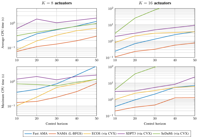
Figure 2: Oscillating masses, average and maximum CPU time (in seconds) for increasing prediction horizon and $50$ randomly selected initial states. First column: $K=8$ actuators. Second column: $K=16$ actuators. Fast AMA and NAMA were stopped as soon as $\|R_{\gamma}(y^{k})\|_{\infty}\leq\epsilon_{\textrm{tol}}=10^{-4}$.

VIII Conclusions

In this work we presented NAMA, a line-search method for minimizing the sum of two convex functions, one of which is assumed to be strongly convex, while the other is composed with a linear transformation. The method is an extension of the classical alternating minimization algorithm (AMA), performing an additional line-search step over the alternating minimization envelope associated with the problem. By appropriately selecting the line-search directions, for example according to quasi-Newton methods for solving the optimality conditions $R_{\gamma}(y)=0$, we have shown that the algorithm converges superlinearly provided that ordinary second-order sufficiency conditions hold for the envelope function at the (unique) dual solution. At the same time, the algorithm possesses the same global sublinear and local linear convergence rates as AMA. Numerical experiments with the proposed method on linear MPC problems suggest that NAMA is able to significantly speed up the convergence of AMA, comparing favorably against its accelerated variant and other state-of-the-art solvers even when limited-memory methods, such as L-BFGS, are used to compute the search directions.

Lemma .1.

Let $y,w\in{{\rm I\mathchoice{}{}{}{}R}}^{m}$ and $\gamma>0$. Then,

$$\psi(w) {}\geq{}\psi_{\gamma}(y)+\tfrac{\gamma}{2}\|Ax(y)-z_{\gamma}(y)\|^{2}$$ (38)

$$\phantom{{}\geq{}}+\langle{}z_{\gamma}(y)-Ax(y){},{}w-y{}\rangle.$$

Proof.

By (1) we have

$$f(x(y))+f^{\ast}(-A^{\top}w) {}\geq{}-\langle{}Ax(y){},{}w{}\rangle,$$

$$g(z_{\gamma}(y))+g^{\ast}(w) {}\geq{}\langle{}z_{\gamma}(y){},{}w{}\rangle.$$

By summing the two inequalities and using the definition of $\psi_{\gamma}$, after manipulations one obtains the result. ∎

Lemma .2.

For all $y\in{{\rm I\mathchoice{}{}{}{}R}}^{m}$ it holds

$$\tfrac{\mu_{f}}{2}\|x(y)-x_{\star}\|^{2}\leq\psi(y)-\inf\psi.$$

Proof.

From the optimality condition of the problem defining $x(y)$, one obtains $-A^{\top}y\in\partial f(x(y))$. Then, by strong convexity of $f$ one gets

$$f(x(y))-\langle{}A^{\top}y{},{}x_{\star}-x(y){}\rangle+\tfrac{\mu_{f}}{2}\|x(y)-x_{\star}\|^{2}\leq f(x_{\star}).$$

By using (16a) in the above inequality we obtain

$$\tfrac{\mu_{f}}{2}\|x(y)-x_{\star}\|^{2}-\langle{}Ax_{\star}{},{}y{}\rangle{}\leq{}f(x_{\star})+f^{\ast}(-A^{\top}y),$$

By using (1) on $g$ we have instead

$$\langle{}Ax_{\star}{},{}y{}\rangle{}\leq{}g(Ax_{\star})+g^{\ast}(y).$$

By summing the last two inequalities one obtains

$$\tfrac{\mu_{f}}{2}\|x(y)-x_{\star}\|^{2}{}\leq{}f(x_{\star})+g(Ax_{\star})+\psi(y),$$

and the claimed bound follows by strong duality. ∎

Lemma .3.

Suppose that the following hold for (I):

1. $A\operatorname{ri}(\operatorname{dom}f)\cap\operatorname{ri}(\operatorname{dom}g)\neq\emptyset$ (strict feasibility);

2. $0\in\operatorname{ri}\partial(f+g\circ A)(x_{\star})$ (strict complementarity).

Then for any compact set $U$ there is $\kappa>0$ such that

$$\operatorname{dist}(y,Y_{\star}){}\leq{}\kappa{\mathopen{}\left[\operatorname{dist}(-A^{\top}y,\partial f(x_{\star})){}+{}\operatorname{dist}(y,\partial g(Ax_{\star}))\right]\mathclose{}}$$

holds for all $y\in U$.

Proof.

From item 2) it follows that

$$0{}\in{} \operatorname{ri}{\mathopen{}\left[\partial f(x_{\star})+A^{\top}\partial g(Ax_{\star})\right]\mathclose{}}$$

$${}={} \operatorname{ri}\partial f(x_{\star})+A^{\top}\operatorname{ri}\partial g(Ax_{\star}).$$ (39)

In fact, the first inclusion is due to [17, Thm 23.9] in light of item 1), and the equality is due to [17, Thm. 6.6]. Consider $W={\mathopen{}\left\{w{}\mid{}-A^{\top}w\in\partial f(x_{\star})\right\}\mathclose{}}\subseteq{{\rm I\mathchoice{}{}{}{}R}}^{m}$. From (4),

$$Y_{\star}=W\cap\partial g(Ax_{\star}).$$

Furthermore, using (39) we obtain

$$\emptyset\neq{\mathopen{}\left\{w{}\mid{}-A^{\top}w\in\operatorname{ri}\partial f(x_{\star})\right\}\mathclose{}}=\operatorname{ri}W,$$

where the equality is due to [17, Thm. 6.7], and the fact that $\operatorname{ri}W\cap\operatorname{ri}\partial g(Ax_{\star})\neq\emptyset$. By [58, Cor. 5] then, we conclude that $W$ and $\partial g(Ax_{\star})$ are boundedly linearly regular: for any compact set $U$ there is $\alpha>0$ such that for all $y\in U$

$$\operatorname{dist}(y,Y_{\star})\leq\alpha\bigl{[}\operatorname{dist}(y,W)+\operatorname{dist}(y,\partial g(Ax_{\star}))\bigr{]}.$$ (40)

Similarly, (39) implies with [58, Cor. 5] that the sets $L={\mathopen{}\left\{(w,-A^{\top}w){}\mid{}w\in{{\rm I\mathchoice{}{}{}{}R}}^{m}\right\}\mathclose{}}$ and $M={{\rm I\mathchoice{}{}{}{}R}}^{m}\times\partial f(x_{\star})$ are boundedly linearly regular. Observe that

$$L\cap M={\mathopen{}\left\{(w,-A^{\top}w){}\mid{}-A^{\top}w\in\partial f(x_{\star})\right\}\mathclose{}}.$$

Therefore, there is $\beta>0$ such that for all $y\in U$

$$\operatorname{dist}(y,W) {}\leq{}\operatorname{dist}((y,-A^{\top}y),L\cap M)$$

$${}\leq{}\beta[\operatorname{dist}((y,-A^{\top}y),L){{}+}\operatorname{dist}((y,-A^{\top}y),M)]$$

$${}={}\beta\operatorname{dist}(-A^{\top}y,\partial f(x_{\star})),$$

where the second inequality is due to bounded linear regularity of $L$ and $M$, while the equality holds since $(y,-A^{\top}y)\in L$ and $\operatorname{dist}((y,-A^{\top}y),M)=\operatorname{dist}(-A^{\top}y,\partial f(x_{\star}))$ for any $y$. Using the above inequality in (40) yields the result. ∎

Lemma .4 (Twice differentiability of $f^{\ast}$).

Suppose that $f$ satisfies Item 1) for the primal-dual solution $(x_{\star},y_{\star})$. Then $f^{\ast}$ is of class $\mathcal{C}^{2}$ around $y_{\star}$, with

$$\nabla^{2}f^{\ast}(y_{\star}){}={}H_{f}^{\dagger}.$$

Proof.

From [20, Thm. 13.21] we know that $f^{\ast}$ is twice epi-differentiable at $v$ for $x\in\partial f^{\ast}(v)$ iff $f$ is twice epi-differentiable at $x$ for $v$, with the relation

$${\rm d}^{2}f^{\ast}{(}{v}{|}{x}{)}{[}{{}}{]}={\mathopen{}\left[{\rm d}^{2}f{(}{x}{|}{v}{)}{[}{{}}{]}\right]\mathclose{}}^{\ast}.$$ (41)

The cited proof trivially extends to strict twice differentiability, and in fact $f^{\ast}$ turns out to be strictly twice epi-differentiable at $x_{\star}$. Since $\operatorname{range}(H_{f})+S_{f}^{\bot}={{\rm I\mathchoice{}{}{}{}R}}^{n}$, by applying (41) to (26) and conjugating ${\rm d}^{2}f{(}{x_{\star}}{|}{-A^{\top}y_{\star}}{)}{[}{{}}{]}$ by means of [18, Prop. E.3.2.1] we obtain that function $f^{\ast}$ has purely quadratic second epi-derivative (as opposed to generalized quadratic)

$${\rm d}^{2}f^{\ast}{(}{-A^{\top}y_{\star}}{|}{x_{\star}}{)}{[}{w}{]}{}={}\langle{}\smash{(\operatorname{\Pi}_{S_{f}}H_{f}\operatorname{\Pi}_{S_{f}})^{\dagger}w}{},{}w{}\rangle{}\mathrel{{}\mathop{{=}\vphantom{\leq}}\limits^{\text{\clap{\eqref{eq:H}}}}}{}\langle{}\smash{H^{\dagger}_{f}}w{},{}w{}\rangle$$

which is everywhere finite in particular. The proof now follows from [25, Cor. 4.7]. ∎

With similar reasonings, the following result easily follows.

Lemma .5 (Twice epi-differentiability of $g^{\ast}$).

Suppose that $g$ (strictly) satisfies Item 2) for a primal-dual solution $(x_{\star},y_{\star})$. Then $g^{\ast}$ is (strictly) twice epi-differentiable at $y_{\star}$ for $Ax_{\star}$. More precisely, letting $\bar{S}=S_{g}^{\bot}+\operatorname{range}(H_{g})$,

$${\rm d}^{2}g^{\ast}{(}{y_{\star}}{|}{Ax_{\star}}{)}{[}{{}}{]}{}={}{\mathopen{}\left[{\rm d}^{2}g{(}{Ax_{\star}}{|}{y_{\star}}{)}{[}{{}}{]}\right]\mathclose{}}^{\ast}{}={}\langle{}H_{g}^{\dagger}{}\cdot{}{},{}{}\cdot{}{}\rangle+\delta_{\bar{S}}.$$ (42)

Lorenzo Stella received the Bachelor and Master degrees in Computer Science from the University of Florence (Italy), and the Ph.D. jointly at the IMT School for Advanced Studies, Lucca (Italy) and the Department of Electrical Engineering (ESAT) of KU Leuven (Belgium). His research interests cover large-scale, nonsmooth optimization algorithms with applications to predictive control and machine learning problems.

Andreas Themelis received both Bachelor and Master degrees in Mathematics from the University of Florence, Italy, in 2010 and 2013, respectively. He is currently pursuing a joint Ph.D at the IMT School for Advanced Studies, Lucca (Italy) and the Department of Electrical Engineering (ESAT) of KU Leuven (Belgium). His research currently focuses on (non)convex nonsmooth optimization with particular interest in splitting schemes deriving from monotone operators theory, and stochastic algorithms intended for large-scale structured problems.

Panagiotis (Panos) Patrinos is currently assistant professor at the Department of Electrical Engineering (ESAT) of KU Leuven, Belgium. He received the M.Eng. in Chemical Engineering, M.Sc. in Applied Mathematics and Ph.D. in Control and Optimization from National Technical University of Athens, Greece. After his Ph.D. he held postdoctoral positions at the University of Trento and IMT School of Advanced Studies Lucca, Italy, where he became an assistant professor in 2012. During fall/winter 2014 he held a visiting assistant professor position in the department of electrical engineering at Stanford University. His current research interests are in the theory and algorithms of optimization and predictive control with a focus on large-scale, distributed, stochastic and embedded optimization with a wide range of application areas including smart grids, water networks, aerospace, and machine learning.

References

- [1] G. Stathopoulos, H. Shukla, A. Szucs, Y. Pu, and C. N. Jones, “Operator splitting methods in control,” Foundations and Trends in Systems and Control, vol. 3, no. 3, pp. 249–362, 2016.
- [2] M. Fazel, T. K. Pong, D. Sun, and P. Tseng, “Hankel matrix rank minimization with applications to system identification and realization,” SIAM Journal on Matrix Analysis and Applications, vol. 34, no. 3, pp. 946–977, 2013.
- [3] S. Boyd, N. Parikh, E. Chu, B. Peleato, and J. Eckstein, “Distributed optimization and statistical learning via the alternating direction method of multipliers,” Foundations and Trends in Machine Learning, vol. 3, no. 1, p. 1–122, 2011.
- [4] N. Parikh and S. Boyd, “Proximal algorithms,” Foundations and Trends in Optimization, vol. 1, no. 3, pp. 127–239, 2014.
- [5] P. Tseng, “Applications of a splitting algorithm to decomposition in convex programming and variational inequalities,” SIAM Journal on Control and Optimization, vol. 29, no. 1, pp. 119–138, 1991.
- [6] P.-L. Lions and B. Mercier, “Splitting algorithms for the sum of two nonlinear operators,” SIAM Journal on Numerical Analysis, vol. 16, no. 6, pp. 964–979, 1979.
- [7] A. Beck and M. Teboulle, “A fast iterative shrinkage-thresholding algorithm for linear inverse problems,” SIAM Journal on Imaging Sciences, vol. 2, no. 1, pp. 183–202, 2009.
- [8] Y. Nesterov, “Gradient methods for minimizing composite functions,” Mathematical Programming, vol. 140, no. 1, pp. 125–161, 2013.
- [9] A. Beck and M. Teboulle, “A fast dual proximal gradient algorithm for convex minimization and applications,” Operations Research Letters, vol. 42, no. 1, pp. 1–6, 2014.
- [10] P. Patrinos and A. Bemporad, “Proximal Newton methods for convex composite optimization,” in IEEE Conference on Decision and Control, 2013, pp. 2358–2363.
- [11] L. Stella, A. Themelis, and P. Patrinos, “Forward-backward quasi-Newton methods for nonsmooth optimization problems,” Computational Optimization and Applications, vol. 67, no. 3, pp. 443–487, 2017.
- [12] A. Themelis, L. Stella, and P. Patrinos, “Forward-backward envelope for the sum of two nonconvex functions: Further properties and nonmonotone line-search algorithms,” arXiv preprint arXiv:1606.06256, 2016.
- [13] T. Liu and T. K. Pong, “Further properties of the forward–backward envelope with applications to difference-of-convex programming,” Computational Optimization and Applications, vol. 67, no. 3, pp. 489–520, 2017.
- [14] A. K. Sampathirao, P. Sopasakis, A. Bemporad, and P. Patrinos, “Proximal limited-memory quasi-Newton methods for scenario-based stochastic optimal control,” To appear in Proceedings of the 20th IFAC Congress, 2017.
- [15] P. Patrinos, L. Stella, and A. Bemporad, “Douglas-Rachford splitting: Complexity estimates and accelerated variants,” in 53rd IEEE Conference on Decision and Control, 2014, pp. 4234–4239.
- [16] A. Themelis, L. Stella, and P. Patrinos, “Douglas–Rachford splitting and ADMM for nonconvex optimization: new convergence results and accelerated versions,” arXiv preprint arXiv:1709.05747, 2017.
- [17] R. T. Rockafellar, Convex Analysis. Princeton university press, 1997.
- [18] J.-B. Hiriart-Urruty and C. Lemaréchal, Fundamentals of Convex Analysis. Springer Science & Business Media, 2001.
- [19] H. H. Bauschke and P. L. Combettes, Convex analysis and monotone operator theory in Hilbert spaces. Springer, 2011.
- [20] R. T. Rockafellar and R. J.-B. Wets, Variational analysis. Springer, 2011, vol. 317.
- [21] R. T. Rockafellar, “First- and second-order epi-differentiability in nonlinear programming,” Transactions of the American Mathematical Society, vol. 307, no. 1, pp. 75–108, 1988.
- [22] ——, “Second-order optimality conditions in nonlinear programming obtained by way of epi-derivatives,” Mathematics of Operations Research, vol. 14, no. 3, pp. 462–484, 1989.
- [23] R. A. Poliquin and R. T. Rockafellar, “Amenable functions in optimization,” Nonsmooth optimization: methods and applications (Erice, 1991), pp. 338–353, 1992.
- [24] ——, “Second-order nonsmooth analysis in nonlinear programming,” Recent advances in nonsmooth optimization, pp. 322–349, 1995.
- [25] ——, “Generalized Hessian properties of regularized nonsmooth functions,” SIAM Journal on Optimization, vol. 6, no. 4, pp. 1121–1137, 1996.
- [26] A. Auslender and M. Teboulle, Asymptotic cones and functions in optimization and variational inequalities. Springer, 2003.
- [27] Y. Nesterov, “A method of solving a convex programming problem with convergence rate ,” Soviet Mathematics Doklady, vol. 27, no. 2, pp. 372–376, 1983.
- [28] ——, Introductory lectures on convex optimization: A basic course. Springer, 2003, vol. 87.
- [29] M. Powell, “A hybrid method for nonlinear equations,” Numerical Methods for Nonlinear Algebraic Equations, pp. 87–144, 1970.
- [30] C. G. Broyden, “A class of methods for solving nonlinear simultaneous equations,” Mathematics of Computation, vol. 19, no. 92, pp. 577–593, 1965.
- [31] R. H. Byrd and J. Nocedal, “A tool for the analysis of quasi-Newton methods with application to unconstrained minimization,” SIAM Journal on Numerical Analysis, vol. 26, no. 3, pp. 727–739, 1989.
- [32] D. C. Liu and J. Nocedal, “On the limited memory BFGS method for large scale optimization,” Mathematical Programming, vol. 45, no. 1-3, pp. 503–528, 1989.
- [33] J. Nocedal, “Updating quasi-Newton matrices with limited storage,” Mathematics of computation, vol. 35, no. 151, pp. 773–782, 1980.
- [34] J. Nocedal and S. Wright, Numerical Optimization, 2nd ed. New York: Springer, 2006.
- [35] R. T. Rockafellar, “A dual approach to solving nonlinear programming problems by unconstrained optimization,” Mathematical Programming, vol. 5, no. 1, pp. 354–373, 1973.
- [36] ——, “Augmented Lagrangians and applications of the proximal point algorithm in convex programming,” Mathematics of operations research, vol. 1, no. 2, pp. 97–116, 1976.
- [37] M. R. Hestenes, “Multiplier and gradient methods,” Journal of optimization theory and applications, vol. 4, no. 5, pp. 303–320, 1969.
- [38] M. J. D. Powell, “A method for nonlinear constraints in minimization problems,” in Optimization, R. Fletcher, Ed. New York: Academic Press, 1969, pp. 283–298.
- [39] D. P. Bertsekas, Convex optimization algorithms. Athena Scientific, 2015.
- [40] W. Li, “Error bounds for piecewise convex quadratic programs and applications,” SIAM Journal on Control and Optimization, vol. 33, no. 5, pp. 1510–1529, 1995.
- [41] D. Drusvyatskiy and A. S. Lewis, “Error bounds, quadratic growth, and linear convergence of proximal methods,” To appear in Mathematics of Operations Research, 2017.
- [42] A. L. Dontchev and R. T. Rockafellar, “Implicit functions and solution mappings,” Springer Monogr. Math., 2009.
- [43] F. Schöpfer, “Linear convergence of descent methods for the unconstrained minimization of restricted strongly convex functions,” SIAM Journal on Optimization, vol. 26, no. 3, pp. 1883–1911, 2016.
- [44] Z. Zhou and A. M.-C. So, “A unified approach to error bounds for structured convex optimization problems,” Mathematical Programming, vol. 165, no. 2, pp. 689–728, 2017.
- [45] F. J. Aragón Artacho and M. H. Geoffroy, “Characterization of metric regularity of subdifferentials,” Journal of Convex Analysis, vol. 15, no. 2, pp. 365–380, 2008.
- [46] D. S. Bernstein, Matrix mathematics: theory, facts, and formulas. Princeton University Press, 2009.
- [47] F. Facchinei and J.-S. Pang, Finite-Dimensional Variational Inequalities and Complementarity Problems. Springer, 2003, vol. 2.
- [48] A. Themelis and P. Patrinos, “SuperMann: a superlinearly convergent algorithm for finding fixed points of nonexpansive operators,” arXiv preprint arXiv:1609.06955, 2016.
- [49] P. Patrinos and A. Bemporad, “An accelerated dual gradient-projection algorithm for embedded linear model predictive control,” IEEE Transactions on Automatic Control, vol. 59, no. 1, pp. 18–33, 2014.
- [50] P. Giselsson and S. Boyd, “Metric selection in fast dual forward–backward splitting,” Automatica, vol. 62, pp. 1–10, 2015.
- [51] A. Bemporad, A. Casavola, and E. Mosca, “Nonlinear control of constrained linear systems via predictive reference management,” IEEE transactions on Automatic Control, vol. 42, no. 3, pp. 340–349, 1997.
- [52] S. Richter, C. N. Jones, and M. Morari, “Certification aspects of the fast gradient method for solving the dual of parametric convex programs,” Mathematical Methods of Operations Research, vol. 77, no. 3, pp. 305–321, 2013.
- [53] Y. Pu, M. N. Zeilinger, and C. N. Jones, “Complexity certification of the fast alternating minimization algorithm for linear MPC,” IEEE Transactions on Automatic Control, vol. 62, no. 2, pp. 888–893, 2017.
- [54] H. J. Ferreau, C. Kirches, A. Potschka, H. G. Bock, and M. Diehl, “qpOASES: A parametric active-set algorithm for quadratic programming,” Mathematical Programming Computation, vol. 6, no. 4, pp. 327–363, 2014.
- [55] A. Domahidi, E. Chu, and S. Boyd, “ECOS: An SOCP solver for embedded systems,” in European Control Conference (ECC), 2013, pp. 3071–3076.
- [56] K.-C. Toh, M. J. Todd, and R. H. Tütüncü, “SDPT3 – a MATLAB software package for semidefinite programming, version 1.3,” Optimization methods and software, vol. 11, no. 1-4, pp. 545–581, 1999.
- [57] J. F. Sturm, “Using SeDuMi 1.02, a MATLAB toolbox for optimization over symmetric cones,” Optimization methods and software, vol. 11, no. 1-4, pp. 625–653, 1999.
- [58] H. H. Bauschke, J. M. Borwein, and W. Li, “Strong conical hull intersection property, bounded linear regularity, Jameson’s property (G), and error bounds in convex optimization,” Mathematical Programming, vol. 86, no. 1, pp. 135–160, 1999.