Generalized Taylor operators and Hermite subdivision schemes

Abstract

Hermite subdivision schemes act on vector valued data that is not only considered as functions values in $\mathbb{R}^{r}$, but as consecutive derivatives, which leads to a mild form of level dependence of the scheme. Previously, we have proved that a property called spectral condition or sum rule implies a factorization in terms of a generalized difference operator that gives rise to a “difference scheme” whose contractivity governs the convergence of the scheme. But many convergent Hermite schemes, for example, those based on cardinal splines, do not satisfy the spectral condition. In this paper, we generalize the property in a way that preserves all the above advantages: the associated factorizations and convergence theory. Based on these results, we can include the case of cardinal splines and also enables us to construct new types of convergent Hermite subdivision schemes.

1 Introduction

Subdivision schemes, as established in [1], are efficient tools for building curves and surfaces with applications in design, creation of images and motion control. For vector subdivision schemes, cf. [8, 9, 19], it is not so straightforward to prove more than the Hölder regularity of the limit function, due to the more complex nature of the underlying factorizations. On the other hand, Hermite subdivision schemes [7, 10, 11, 12, 13] produce function vectors that consist of consecutive derivatives of a certain function, so that the notion of convergence automatically includes regularity of the leading component of the limit. Such schemes have even been considered also on manifolds recently [20] and have also been used for wavelet constructions [5]. While vector subdivision schemes are quite well–understood, nevertheless there are still surprisingly many open questions left in Hermite subdivision. In particular, a characterization of convergence in terms of factorization and contractivity is still missing.

In previous papers [6, 15, 16], we established an equivalence between a so–called spectral condition and operator factorizations that transform a Hermite scheme into a vector scheme for which analysis tools are available. Under this transformation, the usual convergence of the vector subdivision scheme implies convergence for the Hermite scheme and thus regularity of the limit function. It was even conjectured for some time that the spectral condition, sometimes also called the sum rules [2, 11] of the Hermite subdivision scheme, might be necessary for convergence.

In this paper we show, among others results, that this conjecture does not hold true. We define a new set of significantly more general spectral conditions, called spectral chains, that widely generalize the classical spectral condition from [6] and show that these spectral conditions are more or less equivalent to the existence of a factorization with respect to respective generalized Taylor operators and allow for a description of convergence by means of contractivity. We then define a process that allows us to construct Hermite subdivision schemes of arbitrary regularity with guaranteed convergence and, in particular, give examples of convergent Hermite subdivision schemes that do not satisfy the spectral condition. In addition, our new method can be applied to an example based on B–splines and their derivatives which was one of the first examples of a convergent Hermite subdivision scheme that does not satisfy the spectral condition, [14].

The paper is organized as follows: after introducing some basic notation and the concept of convergent vector and Hermite subdivision schemes, we introduce the new concept of chains and generalized Taylor operators in Section 4 and use them for the factorization of subdivision operators in Section 4. These results allow us to extend the known results about the convergence of the Hermite subdivision schemes to this more general case in Section 5. Section 6 is devoted to the construction of a convergent Hermite subdivision scheme emerging from a properly constructed contractive vector subdivision scheme by reversing the factorization process, even in the generality provided by generalized Taylor operators. Finally, we give some examples of the results of such constructions in Section 7, and also provide a new approach for the aforementioned spline case.

2 Notation and fundamental concepts

Vectors in $\mathbb{R}^{r}$, $r\in\mathbb{N}$, will generally be labeled by lowercase boldface letters: ${\boldsymbol{y}}=\left[y_{j}\right]_{j=0,\dots,r-1}$ or ${\boldsymbol{y}}=\left[y^{(j)}\right]_{j=0,\dots,r-1}$, where the latter notation is used to highlight the fact that in Hermite subdivision the components of the vectors correspond to derivatives. Matrices in $\mathbb{R}^{r\times r}$ will be written as uppercase boldface letters, such as ${\boldsymbol{A}}=\left[a_{jk}\right]_{j,k=0,\dots,r-1}$. The space of polynomials in one variable of degree at most $n$ will be written as $\Pi_{n}$, while $\Pi$ will denote the space of all polynomials. Vector sequences will be considered as functions from $\mathbb{Z}$ to $\mathbb{R}^{r}$ and the vector space of all such functions will be denoted by $\ell(\mathbb{Z},\mathbb{R}^{r})$ or $\ell^{r}(\mathbb{Z})$. For ${\boldsymbol{y}}(\cdot)\in\ell(\mathbb{Z},\mathbb{R}^{r})$, the forward difference is defined as $\Delta{\boldsymbol{y}}(\alpha):={\boldsymbol{y}}(\alpha+1)-{\boldsymbol{y}}(\alpha)$, $\alpha\in\mathbb{Z}$, and iterated to $\Delta^{i+1}{\boldsymbol{y}}:=\Delta\left(\Delta^{i}{\boldsymbol{y}}\right)=\Delta^{i}{\boldsymbol{y}}(\cdot+1)-\Delta^{i}{\boldsymbol{y}}(\cdot)$, $i\geq 0$.

Given a finitely supported sequence of matrices ${\boldsymbol{A}}=\left({\boldsymbol{A}}(\alpha)\right)_{\alpha\in\mathbb{Z}}\in\ell^{r\times r}(\mathbb{Z})$, called the mask of the subdivision scheme, we define the associated stationary subdivision operator

$$S_{\boldsymbol{A}}:{\boldsymbol{c}}\mapsto\sum_{\beta\in\mathbb{Z}}{\boldsymbol{A}}(\cdot-2\beta)\,{\boldsymbol{c}}(\beta),\qquad{\boldsymbol{c}}\in\ell^{r}(\mathbb{Z}).$$

The iteration of subdivision operators $S_{{\boldsymbol{A}}_{n}}$, $n\in\mathbb{N}$, is called a subdivision scheme and consists of the successive applications of level-dependent subdivision operators, acting on vector valued data, $S_{{\boldsymbol{A}}_{n}}:\ell^{r}\left(\mathbb{Z}\right)\to\ell^{r}\left(\mathbb{Z}\right)$, defined as

$${\boldsymbol{c}}_{n+1}(\alpha)=S_{{\boldsymbol{A}}_{n}}{\boldsymbol{c}}_{n}(\alpha):=\sum_{\beta\in\mathbb{Z}}{\boldsymbol{A}}_{n}\left(\alpha-2\beta\right)\,{\boldsymbol{c}}_{n}(\beta),\qquad\alpha\in\mathbb{Z},\qquad{\boldsymbol{c}}\in\ell^{r}\left(\mathbb{Z}\right).$$ (1)

An important algebraic tool for stationary subdivision operators is the symbol of the mask, which is the matrix valued Laurent polynomial

$${\boldsymbol{A}}^{*}(z):=\sum_{\alpha\in\mathbb{Z}}{\boldsymbol{A}}(\alpha)\,z^{\alpha},\qquad z\in\mathbb{C}\setminus\{0\}.$$ (2)

We will focus our interest on two kinds of such schemes, the first one being “traditional” vector subdivision schemes in the sense of [1], where ${\boldsymbol{A}}_{n}$ is independent of $n$, i.e., ${\boldsymbol{A}}_{n}(\alpha)={\boldsymbol{A}}(\alpha)$ for any $\alpha\in\mathbb{Z}$ and any $n\geq 0$. In the following, such schemes for which an elaborate theory of convergence exists, will simply be called a vector scheme. Their convergence is defined in the following way.

Definition 1

Let $S_{\boldsymbol{A}}:\ell^{r}(\mathbb{Z})\to\ell^{r}(\mathbb{Z})$ be a vector subdivision operator. The operator is $C^{p}$–convergent, $p\geq 0$, if for any data ${\boldsymbol{g}}_{0}\in\ell^{r}(\mathbb{Z})$ and corresponding sequence of refinements ${\boldsymbol{g}}_{n}=S_{\boldsymbol{A}}^{n}{\boldsymbol{g}}_{0}$ there exists a function $\psi_{\boldsymbol{g}}\in C^{p}\left(\mathbb{R},\mathbb{R}^{r}\right)$ such that for any compact $K\subset\mathbb{R}$ there exists a sequence $\varepsilon_{n}$ with limit $0$ that satisfies

$$\max_{\alpha\in\mathbb{Z}\cap 2^{n}K}\left\|{\boldsymbol{g}}_{n}(\alpha)-\psi_{\boldsymbol{g}}\left(2^{-n}\alpha\right)\right\|_{\infty}\leq\varepsilon_{n}.$$ (3)

As the second type of, now even level–dependent, schemes we consider the Hermite scheme where ${\boldsymbol{A}}_{n}(\alpha)={\boldsymbol{D}}^{-n-1}{\boldsymbol{A}}(\alpha){\boldsymbol{D}}^{n}$ for $\alpha\in\mathbb{Z}$ and $n\geq 0$ with the diagonal matrix ${\boldsymbol{D}}:=\begin{bmatrix}1\\ &\frac{1}{2}\\ &&\ddots\\ &&&\frac{1}{2^{d}}\ \end{bmatrix}$. In this case $r=d+1$ and for $k=0,\ldots,d$ the k-th component of ${\boldsymbol{c}}_{n}(\alpha)$ corresponds to an approximation of the k-th derivative of some function $\varphi_{n}$ at $\alpha 2^{-n}$. Starting from an initial sequence ${\boldsymbol{c}}_{0}$, a Hermite scheme can be rewritten

$${\boldsymbol{D}}^{n+1}\,{\boldsymbol{c}}_{n+1}(\alpha)={\boldsymbol{D}}^{n+1}\,S_{{\boldsymbol{A}}}{\boldsymbol{D}}^{n}{\boldsymbol{c}}_{n}(\alpha)=\sum_{\beta\in\mathbb{Z}}{\boldsymbol{A}}\left(\alpha-2\beta\right)\,{\boldsymbol{D}}^{n}\,{\boldsymbol{c}}_{n}(\beta),\qquad\alpha\in\mathbb{Z},\quad n\geq 0.$$ (4)

Convergence of Hermite schemes is a little bit more intricate and defined as follows.

Definition 2

Let ${\boldsymbol{A}}\in\ell^{(d+1)\times(d+1)}(\mathbb{Z})$ be a mask and $H_{\boldsymbol{A}}$ the associated Hermite subdivision scheme on $\ell^{d+1}(\mathbb{Z})$ as defined in (4). The scheme is convergent if for any data ${\boldsymbol{f}}_{0}\in\ell^{d+1}(\mathbb{Z})$ and the corresponding sequence of refinements ${\boldsymbol{f}}_{n}=[f_{n}^{(0)},\ldots,f_{n}^{(d)}]^{T}$, there exists a function $\Phi=[\phi_{i}]_{0\leq i\leq d}\in C\left(\mathbb{R},\mathbb{R}^{d+1}\right)$ such that for any compact $K\subset\mathbb{R}$ there exists a sequence $\varepsilon_{n}$ with limit $0$ which satisfies

$$\max_{0\leq i\leq d}\max_{\alpha\in\mathbb{Z}\cap 2^{n}K}\left|f_{n}^{(i)}(\alpha)-\phi_{i}\left(2^{-n}\alpha\right)\right|\leq\varepsilon_{n}.$$ (5)

The scheme $H_{\boldsymbol{A}}$ is said to be $C^{p}$–convergent with $p\geq d$ if moreover $\phi_{0}\in C^{p}\left(\mathbb{R},\mathbb{R}\right)$ and

$$\phi_{0}^{(i)}=\phi_{i},\quad 0\leq i\leq d.$$

Remark 3

Since the intuition of Hermite subdivision schemes is to iterate on function values and derivatives, it usually only makes sense to consider $C^{p}$–convergence for $p\geq d$. Note, however, that the case $p>d$ leads to additional requirements.

3 Generalized Taylor operators and chains

In this section, we introduce the concept of generalized Taylor operators and show that they form the basis of symbol factorizations. The first definition concerns vectors of almost monic polynomials of increasing degree.

Definition 4

By $\mathbb{V}_{d}$ we denote the set of all vectors ${\boldsymbol{v}}$ of polynomials in $\Pi_{d}$ with the property that

$${\boldsymbol{v}}=\left[\begin{array}[]{c}v_{d}\\ \vdots\\ v_{0}\end{array}\right],\qquad v_{j}=\frac{1}{j!}(\cdot)^{j}+u_{j}\in\Pi_{j},\qquad u_{j}\in\Pi_{j-1}.$$ (6)

A vector in $\mathbb{V}_{d}$ thus consists of polynomials $v_{j}$ of degree exactly $j$ whose leading coefficient is normalized to $\frac{1}{j!}$, and the remaining part of the polynomial $v_{j}$ of lower degree is denoted by $u_{j}$.

Note that in (6) we always have $v_{0}=1$ and $u_{0}=0$. Also keep in mind that the vectors ${\boldsymbol{v}}$ are indexed in a reversed order, but referring directly to the degree of the object, this notion is more comprehensible.

We will use the convenient notation of Pochhammer symbols $(\cdot)_{j}\in\Pi_{j}$, $j\geq 0$, in the following way:

$$(\cdot)_{0}:=1,\qquad(\cdot)_{j}:=\prod_{k=0}^{j-1}(\cdot-k),\quad j\geq 1,\qquad\text{ and }\qquad[\cdot]_{j}:=\frac{1}{j!}(\cdot)_{j},\quad j\geq 0.$$ (7)

These polynomials satisfy

$$\Delta(\cdot)_{j}=j\,(\cdot)_{j-1},\qquad\Delta[\cdot]_{j}=[\cdot]_{j-1}.$$ (8)

Both $\left\{(\cdot)_{0},\dots,(\cdot)_{j}\right\}$ and $\left\{[\cdot]_{0},\dots,[\cdot]_{j}\right\}$ are bases of $\Pi_{j}$ and allow us to write the Newton interpolation formula of degree $d$ at $0,\dots,d$ in the form

$$x^{j}=\sum_{k=0}^{j}\frac{1}{k!}\left(\Delta^{k}(\cdot)^{j}\right)(0)\,(x)_{k}=\sum_{k=0}^{j}\left(\Delta^{k}(\cdot)^{j}\right)(0)\,[x]_{k};$$

then, since $\Delta^{j}(\cdot)^{j}=j!$, we have that

$$\frac{1}{j!}(\cdot)^{j}=[\cdot]_{j}+\sum_{k=0}^{j-1}\frac{\left(\Delta^{k}(\cdot)^{j}\right)(0)}{j!}\,[x]_{k}$$

which implies that

$${\boldsymbol{v}}\in\mathbb{V}_{d}\qquad\Leftrightarrow\qquad v_{j}=[\cdot]_{j}+u_{j},\qquad u_{j}\in\Pi_{j-1}\quad j=0,\ldots,d.$$ (9)

We will use this form in the future to write each ${\boldsymbol{v}}\in\mathbb{V}_{d}$ as

$${\boldsymbol{v}}=\left[\begin{array}[]{c}{[\cdot]_{d}}\\ \vdots\\ {[\cdot]_{0}}\end{array}\right]+{\boldsymbol{u}}.$$ (10)

Generalizing the Taylor operators operating on vector functions $\mathbb{R}\to\mathbb{R}^{d+1}$ introduced in [6, 15], we define the following concept.

Definition 5

A generalized incomplete Taylor operator is an operator of the form

$$T_{d}:=\begin{bmatrix}\Delta&-1&*&\dots&*\\ &\ddots&\ddots&\ddots&\vdots\\ &&\ddots&\ddots&*\\ &&&\Delta&-1\\ &&&&1\end{bmatrix}=\begin{bmatrix}\Delta I&\\ &1\end{bmatrix}+\left[t_{jk}\right]_{j,k=0,\dots,d},$$ (11)

where $t_{j,j+1}=-1$ and $t_{jk}=0$ for $k\leq j$. In the same way, the generalized complete Taylor operator is of the form

$$\widetilde{T}_{d}:=\begin{bmatrix}\Delta&-1&*&\dots&*\\ &\ddots&\ddots&\ddots&\vdots\\ &&\ddots&\ddots&*\\ &&&\Delta&-1\\ &&&&\Delta\end{bmatrix}=\Delta I+\left[t_{jk}\right]_{j,k=0,\dots,d}.$$ (12)

Remark 6

The Taylor operator becomes generalized for $d\geq 2$, otherwise we simply recover the classical case, see Example 16.

Lemma 7

Let ${\boldsymbol{v}}:=[v_{d},\ldots,v_{0}]^{T}$ be a vector of polynomials in $\Pi^{d+1}$ with $v_{0}=1$. Then ${\boldsymbol{v}}\in\mathbb{V}_{d}$ if and only if there exists a generalized complete Taylor operator $\widetilde{T}_{d}$ such that $\widetilde{T}_{d}{\boldsymbol{v}}=0$.

Proof:  For “$\Leftarrow$” suppose that $\widetilde{T}_{d}{\boldsymbol{v}}=0$ and let us prove inductively for $j=0,\dots,d$, that $v_{j}=[\cdot]_{j}+u_{j}$, for appropriate $u_{j}\in\Pi_{j-1}$. The assumption $v_{0}=1$ ensures that for $j=0$ by simply setting $u_{0}=0$. Now, for $0\leq j<d$, we assume that $v_{j+1}$ is of degree $m\geq 0$ and write it in the basis $\left\{[\cdot]_{0},\ldots,[\cdot]_{m}\right\}$ as

$$v_{j+1}=\sum_{k=0}^{m}c_{k}[\cdot]_{k}=\sum_{k=j+2}^{m}c_{k}[\cdot]_{k}+c_{j+1}[\cdot]_{j+1}+q,$$

with $q\in\Pi_{j}$, hence $\Delta q\in\Pi_{j-1}$. By induction, we suppose that $v_{j}=[\cdot]_{j}+u_{j}$, $u_{j}\in\Pi_{j-1}$ and $v_{k}\in\Pi_{k}$ for $k=0,\ldots,j-1$. Then $\widetilde{T}_{d}{\boldsymbol{v}}=0$ implies at row $d-j-1$ that

$$0 = \Delta v_{j+1}-v_{j}+\sum_{k=0}^{j-1}t_{d-j-1,d-k}v_{k}$$

$$= \sum_{k=j+2}^{m}c_{k}[\cdot]_{k-1}+c_{j+1}[\cdot]_{j}+\Delta q-[\cdot]_{j}-u_{j}+\sum_{k=0}^{j-1}t_{d-j-1,d-k}v_{k}$$

$$= \sum_{k=j+1}^{m-1}c_{k+1}[\cdot]_{k}+\left(c_{j+1}-1\right)[\cdot]_{j}+u,\qquad u\in\Pi_{j-1},$$

and comparison of coefficients yields $c_{j+2}=\cdots=c_{m}=0$ as well as $c_{j+1}=1$, hence $v_{j+1}=[\cdot]_{j+1}+u_{j+1}$ with $u_{j+1}\in\Pi_{j}$, which advances the induction hypothesis.

For the converse “$\Rightarrow$”, we note that for any ${\boldsymbol{v}}\in\mathbb{V}_{d}$ we have that for $j\geq 1$

$$\Delta v_{j}-v_{j-1}=[\cdot]_{j-1}+\Delta u_{j}-[\cdot]_{j-1}-u_{j-1}=\Delta u_{j}-u_{j-1}\in\Pi_{j-2}$$

and since $\left\{v_{0},\ldots,v_{j-2}\right\}$ is a basis of $\Pi_{j-2}$, the polynomial $\Delta v_{j}-v_{j-1}$ can be uniquely written as

$$c_{0}v_{0}+\cdots+c_{j-2}v_{j-2}=-\sum_{\ell=d-j+2}^{d}t_{d-j,\ell}\,v_{d-\ell}$$

which defines the remaining entries of row $d-j$ of $\widetilde{T}_{d}$ in a unique way such that $\widetilde{T}_{d}{\boldsymbol{v}}=0$. $\Box$

The last observation in the above proof can be formalized as follows.

Corollary 8

For each ${\boldsymbol{v}}\in\mathbb{V}_{d}$ there exists a unique generalized complete Taylor operator $\widetilde{T}_{d}$ such that $\widetilde{T}_{d}{\boldsymbol{v}}=0$.

Definition 9

The generalized Taylor operator of Corollary 8, uniquely defined by

$$\widetilde{T}({\boldsymbol{v}})\,{\boldsymbol{v}}=0,$$ (13)

is called the annihilator of ${\boldsymbol{v}}\in\mathbb{V}_{d}$ and written as $\widetilde{T}({\boldsymbol{v}})$. We can skip the subscript “$d$” because it is directly given by the dimension of ${\boldsymbol{v}}$.

Definition 10

A chain of length $d+1$ is a finite sequence ${\boldsymbol{V}}:=[{\boldsymbol{v}}_{0},\dots,{\boldsymbol{v}}_{d}]$ of vectors

$${\boldsymbol{v}}_{j}=\begin{bmatrix}v_{j,j}\\ \vdots\\ v_{j,0}\end{bmatrix}=\begin{bmatrix}{[\cdot]_{j}}\\ \vdots\\ {[\cdot]_{0}}\end{bmatrix}+{\boldsymbol{u}}_{j}\in\mathbb{V}_{j},\qquad j=0,\dots,d,$$

that satisfies the compatibility condition

$${\boldsymbol{w}}_{j+1}:=\begin{bmatrix}w_{j+1,1}\\ \vdots\\ w_{j+1,j+1}\\ \end{bmatrix}:=\widetilde{T}({\boldsymbol{v}}_{j})\begin{bmatrix}v_{j+1,j+1}\\ \vdots\\ v_{j+1,1}\end{bmatrix}\in\mathbb{R}^{j+1},\qquad j=0,\dots,d-1.$$ (14)

Remark 11

Compatibility is a strong requirement on the interaction between ${\boldsymbol{v}}_{j}$ and ${\boldsymbol{v}}_{j+1}$. In general, $\widetilde{T}({\boldsymbol{v}}_{j})\begin{bmatrix}v_{j+1,j+1}\\ \vdots\\ v_{j+1,1}\end{bmatrix}$ can only be expected to be a vector of polynomials in $\Pi_{j},\dots,\Pi_{0}$, while compatibility requires all these polynomials to be constants.

Due to and by means of the compatibility condition, chains uniquely define a generalized Taylor operator.

Lemma 12

If ${\boldsymbol{V}}$ is a chain of length $d+1$, then $w_{jj}=1$, $j=1,\dots,d$.

Proof:  Since $v_{j+1,1}=[\cdot]_{1}+c$ for some constant $c$ due to ${\boldsymbol{v}}_{j}\in\mathbb{V}_{j}$, it follows immediately from the definition (14) that

$$w_{j+1,j+1}=\Delta v_{j+1,1}=1,$$

as claimed. $\Box$

Proposition 13

For ${\boldsymbol{V}}$ of length $d+1$ the following statements are equivalent:

1. ${\boldsymbol{V}}$ is a chain of length $d+1$.

2. For $j=1,\dots,d$, we have

   $$\widetilde{T}({\boldsymbol{v}}_{j})=\begin{bmatrix}\widetilde{T}({\boldsymbol{v}}_{j-1})&-{\boldsymbol{w}}_{j}\\ &\Delta\end{bmatrix}=\begin{bmatrix}\Delta&-w_{1,1}&\dots&-w_{j,1}\\ &\Delta&\ddots&\vdots\\ &&\ddots&-w_{j,j}\\ &&&\Delta\end{bmatrix}.$$ (15)

3. $$\widetilde{T}({\boldsymbol{v}}_{d})\begin{bmatrix}{\boldsymbol{v}}_{j}\\ {\boldsymbol{0}}_{d-j}\end{bmatrix}=0,\qquad j=0,\dots,d.$$ (16)

Proof:  To show that 1) $\Rightarrow$ 2), we note that again (14) yields that

$$0 = \widetilde{T}_{j}({\boldsymbol{v}}_{j})\begin{bmatrix}v_{j+1,j+1}\\ \vdots\\ v_{j+1,1}\end{bmatrix}-{\boldsymbol{w}}_{j+1}=\left[\widetilde{T}({\boldsymbol{v}}_{j})\,|\,-{\boldsymbol{w}}_{j+1}\right]\begin{bmatrix}v_{j+1,j+1}\\ \vdots\\ v_{j+1,1}\\ 1\end{bmatrix}$$

$$= \left[\widetilde{T}({\boldsymbol{v}}_{j})\,|\,-{\boldsymbol{w}}_{j+1}\right]\,{\boldsymbol{v}}_{j+1},$$

Since $\widetilde{T}({\boldsymbol{v}}_{j+1})$ is unique, we deduce that

$$\widetilde{T}({\boldsymbol{v}}_{j+1})=\begin{bmatrix}\widetilde{T}({\boldsymbol{v}}_{j})&-{\boldsymbol{w}}_{j+1}\\ &\Delta\end{bmatrix},\qquad j=0,\dots,d-1,$$ (17)

which directly yields (15).

For 2) $\Rightarrow$ 3) we simply notice that

$$\widetilde{T}({\boldsymbol{v}}_{d})\begin{bmatrix}{\boldsymbol{v}}_{j}\\ {\boldsymbol{0}}_{d-j}\end{bmatrix}=\begin{bmatrix}\widetilde{T}({\boldsymbol{v}}_{j})&*\\ {\boldsymbol{0}}&*\end{bmatrix}\begin{bmatrix}{\boldsymbol{v}}_{j}\\ {\boldsymbol{0}}_{d-j}\end{bmatrix}=\begin{bmatrix}\widetilde{T}({\boldsymbol{v}}_{j}){\boldsymbol{v}}_{j}\\ {\boldsymbol{0}}\end{bmatrix}={\boldsymbol{0}},$$

while for 3) $\Rightarrow$ 1) we first observe for $j<d$ that

$${\boldsymbol{0}}=\widetilde{T}({\boldsymbol{v}}_{d})\begin{bmatrix}{\boldsymbol{v}}_{j}\\ {\boldsymbol{0}}_{d-j}\end{bmatrix}=\begin{bmatrix}\widetilde{T}({\boldsymbol{v}}_{d})_{0:j,0:j}{\boldsymbol{v}}_{j}\\ {\boldsymbol{0}}\end{bmatrix}$$

and the uniqueness of the annihilators from Corollary 8 yields that $\widetilde{T}({\boldsymbol{v}}_{d})_{0:j,0:j}=\widetilde{T}({\boldsymbol{v}}_{j})$. This, in turn, implies together with (16) that

$${\boldsymbol{0}}=\widetilde{T}({\boldsymbol{v}}_{d})\begin{bmatrix}{\boldsymbol{v}}_{j+1}\\ {\boldsymbol{0}}\end{bmatrix}=\begin{bmatrix}\widetilde{T}({\boldsymbol{v}}_{j})&-{\boldsymbol{w}}_{j+1}&*\\ &\Delta&*\\ &&*\end{bmatrix}\begin{bmatrix}v_{j+1,j+1}\\ \vdots\\ v_{j+1}\\ 1\\ {\boldsymbol{0}}\end{bmatrix}=\begin{bmatrix}\widetilde{T}({\boldsymbol{v}}_{j})\,\begin{bmatrix}v_{j+1,j+1}\\ \vdots\\ v_{j+1,1}\end{bmatrix}-{\boldsymbol{w}}_{j+1}\\ 0\\ {\boldsymbol{0}}\end{bmatrix}$$

which is the compatibility identity (14), hence ${\boldsymbol{V}}$ is a chain. $\Box$

Definition 14

The unique generalized Taylor operator $\widetilde{T}({\boldsymbol{v}}_{d})$ for a chain ${\boldsymbol{V}}$ will be written as $\widetilde{T}({\boldsymbol{V}})$.

Remark 15

The operator $\widetilde{T}({\boldsymbol{V}})$ of a chain ${\boldsymbol{V}}$ depends only on the last element ${\boldsymbol{v}}_{d}$ of the chain.

Example 16

Let $p_{j}=[\cdot]_{j}+q_{j}$, $q_{j}\in\Pi_{j-1}$, $j=0,\dots,d$, be given. Then

$${\boldsymbol{v}}_{j}=\begin{bmatrix}p_{j},\,p_{j}^{\prime},\,\dots,\,p_{j}^{(j)}\end{bmatrix}^{T}$$

is a chain for the classical complete Taylor operator

$$\widetilde{T}_{C,d}:=\begin{bmatrix}\Delta&-1&-1/2!&-1/3!&\dots&-1/d!\\ &\Delta&-1&-1/2!&\dots&-1/(d-1)!\\ &&\Delta&-1&&\vdots\\ &&&\ddots&\ddots&\vdots\\ &&&&\Delta&-1\\ &&&&&\Delta\end{bmatrix}.$$ (18)

Similarly,

$${\boldsymbol{v}}_{j}=\begin{bmatrix}p_{j},\,\Delta p_{j},\,\dots,\,\Delta^{j}p_{j}\end{bmatrix}^{T}$$

is a chain for the operator

$$\widetilde{T}_{\Delta,d}:=\begin{bmatrix}\Delta&-1&&{\boldsymbol{0}}\\ &\ddots&\ddots\\ &&\ddots&-1\\ &&&\Delta\end{bmatrix}.$$ (19)

Another interesting generalized Taylor operator is

$$\widetilde{T}_{S,d}:=\begin{bmatrix}\Delta&-1&\dots&-1\\ &\ddots&\ddots&\vdots\\ &&\ddots&-1\\ &&&\Delta\end{bmatrix},$$ (20)

whose chains, connected to B–splines, we will consider in Example 42 later.

As a shorthand for the property (16) of Lemma 13 we write $\widetilde{T}_{d}{\boldsymbol{V}}=0$. Then we have the following result.

Lemma 17

For any generalized complete Taylor operator $\widetilde{T}_{d}$ there exists a chain ${\boldsymbol{V}}$ of length $d+1$ such that $\widetilde{T}_{d}{\boldsymbol{V}}=0$.

Proof:  The construction of the chain ${\boldsymbol{V}}$ is carried out inductively. To that end, we recall that if $p\in\Pi$ is of the form $\Delta p=[\cdot]_{k}$ for some $k\in\mathbb{N}$, then $p=[\cdot]_{k+1}+c$ with some $c\in\mathbb{R}$.

Next, let ${\boldsymbol{v}}_{j}\in\mathbb{V}_{j}$, $j=0,\dots,d$, be any solution of

$$0=\widetilde{T}_{d}\begin{bmatrix}{\boldsymbol{v}}_{j}\\ {\boldsymbol{0}}_{d-j}\end{bmatrix}=\begin{bmatrix}\widetilde{T}_{j}&*\\ 0&*\end{bmatrix}\begin{bmatrix}{\boldsymbol{v}}_{j}\\ {\boldsymbol{0}}_{d-j}\end{bmatrix},$$

or, equivalently, of $\widetilde{T}_{j}{\boldsymbol{v}}_{j}=0$. Such a solution can be found by setting $v_{j0}=1$ and then solving, recursively for $k=1,\dots,j$, the equation given by row $j-k$ of the Taylor operator,

$$0=\Delta v_{j,k}-v_{j,k-1}+\sum_{\ell=0}^{k-2}t_{j-k,j-\ell}\,v_{j,\ell}.$$ (21)

Equivalently, this can be written with respect to the basis $\left\{[\cdot]_{0},\ldots,[\cdot]_{k-1}\right\}$ and using $v_{j,k-1}=[\cdot]_{k-1}+u_{j,k-1}$, $u_{j,k-1}\in\Pi_{k-2}$, as

$$0=\Delta v_{j,k}-[\cdot]_{k-1}+\sum_{\ell=0}^{k-2}s_{j-k,\ell}\,[\cdot]_{\ell},\qquad s_{j-k,\ell}\in\mathbb{R},$$

yielding

$$v_{jk}=[\cdot]_{k}+\sum_{\ell=1}^{k-1}s_{j-k,\ell-1}[\cdot]_{\ell}+c_{k0},\qquad k=0,\dots,j,$$

where the constants $c_{k0}\in\mathbb{R}$ can be chosen freely. This process yields polynomial vectors ${\boldsymbol{v}}_{j}\in\mathbb{V}_{j}$ such that $\widetilde{T}_{j}{\boldsymbol{v}}_{j}=0$, $j=0,\dots,d$.

Thus, it follows from the uniqueness of the annihilating Taylor operator from Corollary 8 that $\widetilde{T}_{j}=T({\boldsymbol{v}}_{j})$, and decomposing the identity

$$0=\widetilde{T}({\boldsymbol{v}}_{j+1}){\boldsymbol{v}}_{j+1}=\widetilde{T}_{j+1}{\boldsymbol{v}}_{j+1}=\left[\begin{array}[]{cc}\widetilde{T}({\boldsymbol{v}}_{j})&-{\boldsymbol{w}}\\ 0&\Delta\end{array}\right]{\boldsymbol{v}}_{j+1}$$

yields

$$\widetilde{T}({\boldsymbol{v}}_{j})\left[\begin{array}[]{c}v_{j+1,j+1}\\ \vdots\\ v_{j+1,1}\end{array}\right]={\boldsymbol{w}}=:{\boldsymbol{w}}_{j+1},$$ (22)

which is exactly the compatibility condition (14) needed for ${\boldsymbol{V}}$ to be a chain. $\Box$

Corollary 18

In the chain ${\boldsymbol{V}}$ from Lemma 17 the constant coefficients of the polynomials $v_{jk}$, $j=1,\dots,d$, $k=1,\dots,j$, can be chosen arbitrarily.

Remark 19

The chain associated to a generalized Taylor operator is not at all unique, see also Example 16.

The next result shows that any polynomial vector in $\mathbb{V}_{d}$ can be reached by a chain of length $d+1$.

Proposition 20

For any ${\boldsymbol{v}}\in\mathbb{V}_{d}$ there exists a chain ${\boldsymbol{V}}$ of length $d+1$ with ${\boldsymbol{v}}_{d}={\boldsymbol{v}}$.

Proof:  Again we prove the claim by induction on $d$. The case $d=0$ is trivial as the only chain of length $0$ consists of $v=1$. For the induction step, we choose ${\boldsymbol{v}}\in\mathbb{V}_{d}$, $d>0$ and the associated generalized Taylor operator $\widetilde{T}({\boldsymbol{v}})$ as in Definition 14. Then we know from Lemma 17 that there exists a chain ${\boldsymbol{V}}=\left[{\boldsymbol{v}}_{0},\dots,{\boldsymbol{v}}_{d}\right]$ of length $d+1$ such that $\widetilde{T}({\boldsymbol{v}}){\boldsymbol{V}}=0$. Suppose that ${\boldsymbol{v}}_{d}\neq{\boldsymbol{v}}$ and, in particular, that $v_{d,1}(0)=v_{1}(0)-1$, which is possible according to Corollary 18. With

$${\boldsymbol{v}}=\left[\begin{array}[]{c}{[\cdot]_{d}}\\ \vdots\\ {[\cdot]_{0}}\end{array}\right]+{\boldsymbol{u}},\qquad{\boldsymbol{v}}_{d}=\left[\begin{array}[]{c}{[\cdot]_{d}}\\ \vdots\\ {[\cdot]_{0}}\end{array}\right]+{\boldsymbol{u}}_{d},\qquad u_{0}=u_{d,0}=0,$$

we find that

$$0=\widetilde{T}({\boldsymbol{v}})\left({\boldsymbol{v}}-{\boldsymbol{v}}_{d}\right)=\widetilde{T}({\boldsymbol{v}})\left[\begin{array}[]{c}u_{d}-u_{d,d}\\ \vdots\\ u_{1}-u_{d,1}\\ 0\end{array}\right]=:\widetilde{T}({\boldsymbol{v}})\left[\begin{array}[]{c}{\boldsymbol{v}}^{\prime}\\ 0\end{array}\right]$$

where $u_{1}-u_{d,1}=v_{1}(0)-v_{d,1}(0)=1$. In addition, Lemma 7 yields that ${\boldsymbol{v}}^{\prime}\in\mathbb{V}_{d-1}$ and therefore the decomposition

$$\widetilde{T}({\boldsymbol{v}})=\left[\begin{array}[]{cc}\widetilde{T}({\boldsymbol{v}}^{\prime})&-{\boldsymbol{w}}\\ 0&\Delta\end{array}\right]$$

and

$$0=\widetilde{T}({\boldsymbol{v}}){\boldsymbol{v}}=\left[\begin{array}[]{cc}\widetilde{T}({\boldsymbol{v}}^{\prime})&-{\boldsymbol{w}}\\ 0&\Delta\end{array}\right]\left[\begin{array}[]{c}v_{d}\\ \vdots\\ v_{1}\\ 1\end{array}\right]=\widetilde{T}({\boldsymbol{v}}^{\prime})\left[\begin{array}[]{c}v_{d}\\ \vdots\\ v_{1}\\ 1\end{array}\right]-{\boldsymbol{w}}$$

compatibility between ${\boldsymbol{v}}^{\prime}$ and ${\boldsymbol{v}}$. By the induction hypothesis, there exists a chain ${\boldsymbol{V}}^{\prime}$ of length $d$ with ${\boldsymbol{v}}_{d-1}={\boldsymbol{v}}^{\prime}$ and since ${\boldsymbol{v}}^{\prime}$ is compatible with ${\boldsymbol{v}}$, this chain can be extended to length $d+1$ with ${\boldsymbol{v}}_{d}^{\prime}={\boldsymbol{v}}$. $\Box$

4 Chains and factorizations

We now relate the existence of a spectral chain to factorizations of the subdivision operators, thus extending the results first given in [15] for the classical Taylor operator.

Definition 21

A chain ${\boldsymbol{V}}$ of length $d+1$ is called spectral chain for a vector subdivision scheme with mask ${\boldsymbol{A}}\in\ell^{(d+1)\times(d+1)}(\mathbb{Z})$ if

$$S_{\boldsymbol{A}}\hat{\boldsymbol{v}}_{j}=2^{-j}\hat{\boldsymbol{v}}_{j},\qquad\hat{\boldsymbol{v}}_{j}:=\left[\begin{array}[]{c}{\boldsymbol{v}}_{j}\\ {\boldsymbol{0}}_{d-j}\end{array}\right],\qquad j=0,\dots,d.$$ (23)

We will prove in Theorem 24 that the existence of spectral chains is equivalent to the existence of generalized Taylor factorizations. The main tool for this proof is the following result.

Proposition 22

If ${\boldsymbol{C}}\in\ell^{(d+1)\times(d+1)}(\mathbb{Z})$ is a finitely supported mask for which there exists a chain ${\boldsymbol{V}}$ such that $S_{\boldsymbol{C}}\hat{\boldsymbol{v}}_{j}=0$, $j=0,\dots,d$, then there exists a finitely supported mask ${\boldsymbol{B}}\in\ell^{(d+1)\times(d+1)}(\mathbb{Z})$ such that $S_{\boldsymbol{C}}=S_{\boldsymbol{B}}\,\widetilde{T}({\boldsymbol{V}})$.

Proof:  We follow the idea from [15] and prove by induction on $k$ that the symbol ${\boldsymbol{C}}^{*}(z)$ satisfies

$${\boldsymbol{C}}^{*}(z)={\boldsymbol{B}}_{k}^{*}(z)\begin{bmatrix}\widetilde{T}({\boldsymbol{v}}_{k})^{*}(z)&{\boldsymbol{0}}\\ {\boldsymbol{0}}&{\boldsymbol{I}}\end{bmatrix},\qquad k=0,\dots,d.$$ (24)

with the columnwise written matrix

$${\boldsymbol{B}}_{k}^{*}(z)=\left[{\boldsymbol{b}}_{0}^{*}(z)\cdots{\boldsymbol{b}}_{k}^{*}(z){\boldsymbol{c}}_{k+1}^{*}(z)\cdots{\boldsymbol{c}}_{d}^{*}(z)\right].$$ (25)

The construction makes repeated use of the well known factorization for a scalar subdivision scheme $S_{a}$:

$$\sum_{\alpha\in\mathbb{Z}}a(\alpha-2\beta)=0\qquad\Rightarrow\qquad a^{*}(z)=(z^{-2}-1)b^{*}(z),$$ (26)

see, for example, [1] for proof.

For case $k=0$, the annihilation of the vector $\hat{\boldsymbol{v}}_{0}={\boldsymbol{e}}_{0}=[1,0,\ldots,0]^{T}$ immediately gives the decomposition ${\boldsymbol{c}}_{0}^{*}(z)=\left(z^{-2}-1\right){\boldsymbol{b}}_{0}^{*}(z)$ and therefore

$${\boldsymbol{C}}^{*}(z) = \left[{\boldsymbol{b}}_{0}^{*}(z){\boldsymbol{c}}_{1}^{*}(z)\cdots{\boldsymbol{c}}_{d}^{*}(z)\right]\begin{bmatrix}z^{-2}-1\\ &{\boldsymbol{I}}\end{bmatrix}$$

$$= \left[{\boldsymbol{b}}_{0}^{*}(z){\boldsymbol{c}}_{1}^{*}(z)\cdots{\boldsymbol{c}}_{d}^{*}(z)\right]\begin{bmatrix}\widetilde{T}({\boldsymbol{v}}_{0})^{*}(z)\\ &{\boldsymbol{I}}\end{bmatrix}.$$

Now suppose that (24) holds for some $k\geq 0$. Then the fact that ${\boldsymbol{V}}$ is a chain yields, by means of the compatibility condition

$${\boldsymbol{w}}_{k+1}=\widetilde{T}({\boldsymbol{v}}_{k})\begin{bmatrix}v_{k+1,k+1}\\ \vdots\\ v_{k+1,1}\end{bmatrix}$$

that

$$0=S_{\boldsymbol{C}}\hat{\boldsymbol{v}}_{k+1}=S_{{\boldsymbol{B}}_{k}}\left[\begin{array}[]{cc|c}\widetilde{T}({\boldsymbol{v}}_{k})&&\\ &1&\\ \hline\cr&&{\boldsymbol{I}}\end{array}\right]\begin{bmatrix}{\boldsymbol{v}}_{k+1}\\ {\boldsymbol{0}}\end{bmatrix}=S_{{\boldsymbol{B}}_{k}}\begin{bmatrix}{\boldsymbol{w}}_{k+1}\\ 1\\ {\boldsymbol{0}}\end{bmatrix},$$

or, applying (26) to each row of the preceding equation,

$$\left[{\boldsymbol{b}}_{0}^{*}(z)\cdots{\boldsymbol{b}}_{k}^{*}(z)\right]^{T}{\boldsymbol{w}}_{k+1}+{\boldsymbol{c}}_{k+1}^{*}(z)=\left(z^{-2}-1\right){\boldsymbol{b}}_{k+1}^{*}(z),$$

which is

$${\boldsymbol{c}}_{k+1}^{*}(z)=\left[{\boldsymbol{b}}_{0}^{*}(z)\cdots{\boldsymbol{b}}_{k+1}^{*}(z)\right]^{T}\begin{bmatrix}-{\boldsymbol{w}}_{k+1}\\ z^{-2}-1\end{bmatrix},$$

or

$${\boldsymbol{C}}^{*}(z)=\left[{\boldsymbol{b}}_{0}^{*}(z)\cdots{\boldsymbol{b}}_{k+1}^{*}(z){\boldsymbol{c}}_{k+2}^{*}(z)\cdots{\boldsymbol{c}}_{d}^{*}(z)\right]\begin{bmatrix}\widetilde{T}({\boldsymbol{v}}_{k})^{*}(z)&-{\boldsymbol{w}}_{k+1}&\\ &z^{-2}-1&\\ &&{\boldsymbol{I}}\end{bmatrix}.$$ (27)

Since

$$\widetilde{T}({\boldsymbol{v}}_{k+1})^{*}(z)=\begin{bmatrix}\widetilde{T}({\boldsymbol{v}}_{k})^{*}(z)&-{\boldsymbol{w}}_{k+1}\\ &z^{-2}-1\\ \end{bmatrix},$$

(27) yields (24) with $k$ replaced by $k+1$ and advances the induction hypothesis. $\Box$

Remark 23

Proposition 22 shows that, in the terminology of [3], the generalized Taylor operator is a minimal annihilator for the chain ${\boldsymbol{V}}$ since it annihilates the chain and factors any subdivision operator that does so, too.

Now we can show that the existence of a spectral chain results in the existence of a factorization by means of generalized Taylor operators. Since the Taylor operator corresponds to computing differences, the scheme $S_{\boldsymbol{B}}$ from (28) is often called the difference scheme of $S_{\boldsymbol{A}}$ with respect to the generalized Taylor operator $\widetilde{T}({\boldsymbol{V}})$.

Theorem 24

If $S_{\boldsymbol{A}}$ possesses a spectral chain ${\boldsymbol{V}}$ of length $d+1$ then there exists a finite mask ${\boldsymbol{B}}\in\ell^{(d+1)\times(d+1)}(\mathbb{Z})$ such that

$$\widetilde{T}({\boldsymbol{V}})\,S_{\boldsymbol{A}}=S_{\boldsymbol{B}}\,\widetilde{T}({\boldsymbol{V}}).$$ (28)

Proof:  Since $S_{\boldsymbol{C}}:=\widetilde{T}({\boldsymbol{V}})S_{\boldsymbol{A}}$ has the property that

$$S_{\boldsymbol{C}}\hat{\boldsymbol{v}}_{k}=\widetilde{T}({\boldsymbol{V}})S_{\boldsymbol{A}}{\boldsymbol{v}}_{k}=2^{-k}\widetilde{T}({\boldsymbol{V}}){\boldsymbol{v}}_{k}=0,$$

an application of Proposition 22 proves the claim. $\Box$

Remark 25

For the validity of Theorem 24, which is of a purely algebraic nature, the concrete eigenvalues of the spectral set are irrelevant. Their normalization will play a role, however, as soon as convergence is concerned.

Next, we generalize a result from [16] that serves as a converse of Theorem 24. The proof is a modification of the former.

Theorem 26

Suppose that for a finitely supported mask ${\boldsymbol{A}}\in\ell^{(d+1)\times(d+1)}$ there exists a finitely supported ${\boldsymbol{B}}$ and a generalized incomplete Taylor operator $T_{d}$ such that $T_{d}S_{\boldsymbol{A}}=2^{-d}S_{\boldsymbol{B}}T_{d}$ and $S_{\boldsymbol{B}}{\boldsymbol{e}}_{d}={\boldsymbol{e}}_{d}$. If a chain ${\boldsymbol{V}}$ for $T_{d}$ satisfies

$$S_{\boldsymbol{A}}\hat{\boldsymbol{v}}_{j}\in\mbox{\rm span}\left\{\hat{\boldsymbol{v}}_{0},\dots,\hat{\boldsymbol{v}}_{j}\right\},\qquad j=0,\dots,d,$$ (29)

then there exists a spectral chain ${\boldsymbol{V}}^{\prime}$ for $S_{\boldsymbol{A}}$.

Proof:  Relying on Lemma 17, we choose a chain ${\boldsymbol{V}}$ such that $\widetilde{T}_{d}=\widetilde{T}({\boldsymbol{V}})$, which particularly yields that $T_{d}{\boldsymbol{v}}_{d}={\boldsymbol{e}}_{d}$. Then

$$T_{d}{\boldsymbol{v}}_{d}={\boldsymbol{e}}_{d}=S_{\boldsymbol{B}}{\boldsymbol{e}}_{d}=S_{\boldsymbol{B}}T_{d}{\boldsymbol{v}}_{d}=2^{d}T_{d}S_{\boldsymbol{A}}{\boldsymbol{v}}_{d}$$

implies that $T_{d}\left(2^{-d}{\boldsymbol{v}}_{d}-S_{\boldsymbol{A}}{\boldsymbol{v}}_{d}\right)=0$, hence

$$S_{\boldsymbol{A}}{\boldsymbol{v}}_{d}=2^{-d}{\boldsymbol{v}}_{d}+\tilde{\boldsymbol{v}},\qquad 0=T_{d}\tilde{\boldsymbol{v}}=\begin{bmatrix}\widetilde{T}_{d-1}&*\\ &1\end{bmatrix}\tilde{\boldsymbol{v}},$$

so that $\tilde{v}_{0}=0$ and therefore $\widehat{T}_{d-1}\tilde{\boldsymbol{v}}_{0:d-1}=0$. Since $\hat{\boldsymbol{v}}_{0},\dots,\hat{\boldsymbol{v}}_{d-1}$ form a basis for the kernel of $\widetilde{T}_{d}$ with last component equal to zero, it follows that $\hat{\boldsymbol{v}}\in\mbox{\rm span}\{{\boldsymbol{v}}_{0},\dots,{\boldsymbol{v}}_{d-1}\}$. Making use of the two–slantedness of $S_{\boldsymbol{A}}$, one can literally repeat the arguments of the proof of [16, Theorem 2.11] to conclude that

$$S_{\boldsymbol{A}}\hat{\boldsymbol{v}}_{j}-2^{-j}\hat{\boldsymbol{v}}_{j}\in\mbox{\rm span}\left\{\hat{\boldsymbol{v}}_{0},\dots,\hat{\boldsymbol{v}}_{j-1}\right\},$$

hence $S_{\boldsymbol{A}}\left[\hat{\boldsymbol{v}}_{0},\dots,\hat{\boldsymbol{v}}_{d}\right]=\left[\hat{\boldsymbol{v}}_{0},\dots,\hat{\boldsymbol{v}}_{d}\right]{\boldsymbol{U}}$, where ${\boldsymbol{U}}\in\mathbb{R}^{(d+1)\times(d+1)}$ is an upper triangular matrix with diagonal entries $1,\dots,2^{-d}$. Using the upper triangular ${\boldsymbol{S}}$ such that ${\boldsymbol{S}}^{-1}{\boldsymbol{U}}{\boldsymbol{S}}$ is diagonal, we can then define ${\boldsymbol{V}}^{\prime}$ by $\left[\hat{\boldsymbol{v}}_{0}^{\prime},\dots,\hat{\boldsymbol{v}}_{d}^{\prime}\right]=\left[\hat{\boldsymbol{v}}_{0},\dots,\hat{\boldsymbol{v}}_{d}\right]{\boldsymbol{S}}$, which is a chain since

$$\widetilde{T}({\boldsymbol{v}}_{d})\left(\sum_{k=0}^{j}c_{k}\,\hat{\boldsymbol{v}}_{k}\right)=0,\qquad j=0,\dots,d,$$

due to Proposition 13. $\Box$

5 Convergence

From [15, 16], we know that the Hermite subdivision scheme $H_{\boldsymbol{A}}$ converges to a $C^{d}$ function according to Definition 2 if

1. there exists a scheme $S_{\boldsymbol{B}}$ such that $T_{C,d}S_{\boldsymbol{A}}=2^{-d}S_{\boldsymbol{B}}T_{C,d}$ and $S_{\boldsymbol{B}}$ is convergent with limit function ${\boldsymbol{f}}_{\boldsymbol{c}}={\boldsymbol{e}}_{d}f_{\boldsymbol{c}}$, where ${\boldsymbol{e}}_{d}=[0,\ldots,0,1]^{T}$,

2. there exists a scheme $S_{\widetilde{\boldsymbol{B}}}$ such that $\widetilde{T}_{C,d}S_{\boldsymbol{A}}=2^{-d}S_{\widetilde{\boldsymbol{B}}}\widetilde{T}_{C,d}$ and $S_{\widetilde{\boldsymbol{B}}}$ is contractive.

Note that the normalization with the factor $2^{-d}$ now becomes relevant since it affects the normalization and contractivity property of $S_{\boldsymbol{B}}$ and $S_{\widetilde{\boldsymbol{B}}}$, respectively.

Before we give the results about the convergence replacing $T_{C,d}$ and $\widetilde{T}_{C,d}$ by $T$ and $\widetilde{T}$, respectively, we will now consider conditions to guarantee that $\widetilde{\boldsymbol{B}}$ is the result of such a factorization. To that end, we recall the factorization identity

$$\begin{bmatrix}{\boldsymbol{I}}_{d}\\ &\Delta\end{bmatrix}S_{\boldsymbol{B}}=S_{\widetilde{\boldsymbol{B}}}\begin{bmatrix}{\boldsymbol{I}}_{d}\\ &\Delta\end{bmatrix}$$ (30)

from vector subdivision [19]. This relationship does not depend on the form of the Taylor operator. In terms of symbols, (30) becomes

$$\begin{bmatrix}{\boldsymbol{I}}_{d}&\\ &z^{-1}-1\end{bmatrix}\begin{bmatrix}{\boldsymbol{B}}_{11}^{*}(z)&{\boldsymbol{B}}_{12}^{*}(z)\\ {\boldsymbol{B}}_{21}^{*}(z)&{\boldsymbol{B}}_{22}^{*}(z)\end{bmatrix}=\begin{bmatrix}\widetilde{\boldsymbol{B}}_{11}^{*}(z)&\widetilde{\boldsymbol{B}}_{12}^{*}(z)\\ \widetilde{\boldsymbol{B}}_{21}^{*}(z)&\widetilde{\boldsymbol{B}}_{22}^{*}(z)\end{bmatrix}\begin{bmatrix}{\boldsymbol{I}}_{d}&\\ &z^{-2}-1\end{bmatrix},$$ (31)

hence

$${\boldsymbol{B}}^{*}(z) = \begin{bmatrix}{\boldsymbol{I}}_{d}&\\ &z^{-1}-1\\ \end{bmatrix}^{-1}\begin{bmatrix}\widetilde{\boldsymbol{B}}_{11}^{*}(z)&\widetilde{\boldsymbol{B}}_{12}^{*}(z)\\ \widetilde{\boldsymbol{B}}_{21}^{*}(z)&\widetilde{\boldsymbol{B}}_{22}^{*}(z)\\ \end{bmatrix}\begin{bmatrix}{\boldsymbol{I}}_{d}&\\ &z^{-2}-1\\ \end{bmatrix}$$ (32)

$$= \begin{bmatrix}\widetilde{\boldsymbol{B}}_{11}^{*}(z)&(z^{-2}-1)\,\widetilde{\boldsymbol{B}}_{12}^{*}(z)\\ (z^{-1}-1)^{-1}\widetilde{\boldsymbol{B}}_{21}^{*}(z)&(z+1)\,\widetilde{\boldsymbol{B}}_{22}^{*}(z)\end{bmatrix}.$$

Lemma 27

$S_{\boldsymbol{B}}$ converges to a continuous limit function of the form ${\boldsymbol{f}}_{\boldsymbol{c}}=f_{\boldsymbol{c}}\,{\boldsymbol{e}}_{d}$ if and only if $S_{\widetilde{\boldsymbol{B}}}$ is contractive, $\widetilde{\boldsymbol{B}}_{21}(1)=0$ and $\widetilde{\boldsymbol{B}}_{22}(1)=1$.

Proof:  First, to make ${\boldsymbol{B}}^{*}$ a Laurent polynomial, we must have $\widetilde{\boldsymbol{B}}_{21}^{*}(1)=0$, otherwise $(z^{-1}-1)^{-1}\widetilde{\boldsymbol{B}}_{21}^{*}(z)$ has a pole at $1$. Second, the condition $S_{\boldsymbol{B}}{\boldsymbol{e}}_{d}={\boldsymbol{e}}_{d}$ is equivalent to ${\boldsymbol{B}}^{*}(-1){\boldsymbol{e}}_{d}=0$ and ${\boldsymbol{B}}^{*}(1){\boldsymbol{e}}_{d}=2{\boldsymbol{e}}_{d}$. The first one of these requirements is automatically satisfied according to (32), the second one becomes $2{\boldsymbol{B}}_{22}^{*}(1)=2$. $\Box$

Now we study the convergence of the Hermite scheme whenever we have one of the factorizations: $\widetilde{T}S_{\boldsymbol{A}}=2^{-d}S_{\widetilde{\boldsymbol{B}}}\widetilde{T}$ or $TS_{\boldsymbol{A}}=2^{-d}S_{{\boldsymbol{B}}}T$. To that end, we first recall the one dimensional case of Lemma 3 in [15].

Lemma 28

Given a sequence of refinements ${\boldsymbol{h}}_{n}=\begin{bmatrix}h_{n}^{(0)}\\ h^{(1)}_{n}\end{bmatrix}\in\ell(\mathbb{Z},\mathbb{R}^{2})$ such that

1. there exists a constant $c$ in $\mathbb{R}$ such that $\lim_{n\to+\infty}h_{n}^{(0)}(0)=c$,

2. there exists a function $\xi\in C\left(\mathbb{R},\mathbb{R}\right)$ such that for any compact subset $K$ of $\mathbb{R}$ there exists a sequence $\mu_{n}$ with limit $0$ and

   $$\max_{\alpha\in 2^{n}K\cap\mathbb{Z}}\left|h_{n}^{(1)}(\alpha)-\xi\left(2^{-n}\alpha\right)\right|_{\infty} \leq \mu_{n},$$ (33)

   $$\max_{\alpha\in 2^{n}K\cap\mathbb{Z}}\left|2^{n}\Delta h^{(0)}_{n}(\alpha)-h_{n}^{(1)}(\alpha)\right|_{\infty} \leq \mu_{n}.$$ (34)

Then there exists for any compact $K$ a sequence $\theta_{n}$ with limit $0$ such that the function

$$\varphi(x)=c+\int_{0}^{1}x\,\xi\left(tx\right)dt,\qquad x\in\mathbb{R},$$ (35)

satisfies

$$\max_{\alpha\in 2^{n}K\cap\mathbb{Z}}\left\|h_{n}^{(0)}(\alpha)-\varphi\left(2^{-n}\alpha\right)\right\|\leq\theta_{n},\qquad n\in\mathbb{N}.$$ (36)

Theorem 29

Let ${\boldsymbol{A}},{\boldsymbol{B}}\in\ell^{d+1}(\mathbb{Z})$ be two masks related by the the factorization $T_{d}S_{\boldsymbol{A}}=2^{-d}S_{\boldsymbol{B}}T_{d}$ for some generalized incomplete Taylor operator $T_{d}$.

Suppose that for any initial data ${\boldsymbol{f}}_{0}\in\ell^{d+1}(\mathbb{Z})$ and associated refinement sequence ${\boldsymbol{f}}_{n}$ of the Hermite scheme $H_{\boldsymbol{A}}$,

1. the sequence ${\boldsymbol{f}}_{n}(0)$ converges to a limit ${\boldsymbol{y}}\in\mathbb{R}^{d+1}$,

2. the subdivision scheme $S_{\boldsymbol{B}}$ is $C^{p-d}$–convergent for some $p\geq d$, and that for any initial data ${\boldsymbol{g}}_{0}=T_{d}{\boldsymbol{f}}_{0}$, the limit function $\Psi=\Psi_{\boldsymbol{g}}\in C^{p-d}\left(\mathbb{R},\mathbb{R}^{d+1}\right)$ satisfies

   $$\Psi=\begin{bmatrix}{\boldsymbol{0}}\\ \psi\end{bmatrix},\qquad\psi\in C^{p-d}\left(\mathbb{R},\mathbb{R}\right).$$ (37)

Then $H_{\boldsymbol{A}}$ is $C^{p}$–convergent.

Proof:  The proof is adapted from the proofs in [6, 14]. Given ${\boldsymbol{f}}_{0}\in\ell^{d+1}(\mathbb{Z})$, let ${\boldsymbol{g}}_{0}=T_{d}{\boldsymbol{f}}_{0}$. We define the following two sequences: ${\boldsymbol{f}}_{n+1}={\boldsymbol{D}}^{-n-1}S_{\boldsymbol{A}}({\boldsymbol{D}}{\boldsymbol{f}}_{n})$ and ${\boldsymbol{g}}_{n+1}=S_{\boldsymbol{B}}{\boldsymbol{g}}_{n}$, $n\in\mathbb{N}$. Since $T_{d}S_{\boldsymbol{A}}=2^{-d}S_{\boldsymbol{B}}T_{d}$, we can directly deduce that ${\boldsymbol{g}}_{n}=2^{nd}T_{d}{\boldsymbol{D}}^{n}{\boldsymbol{f}}_{n}$.

With the convergence of ${\boldsymbol{f}}_{n}(0)$, let $y_{i}:=\lim_{n\to+\infty}f_{n}^{(i)}(0)$, $i=0,\ldots,d$. Then we define $\Phi$ recursively beginning with $\phi_{d}=\psi$ and setting

$$\phi_{i}(x)=y_{i}+\int_{0}^{1}x\,\phi_{i+1}(tx)\,dt\qquad i=d-1,\dots,0.$$ (38)

Then $\Phi=[\phi_{i}]_{i=0,\ldots d}$ is continuous with $\phi_{i}^{(d-i)}=\psi$.

Fixing a compact $K\subset\mathbb{R}$, we will prove by a backward finite recursion that for $k=d,d-1,\dots,0$, there exists a sequence $\varepsilon_{n}$ with limit $0$ such that

$$\left|f_{n}^{(k)}(\gamma)-\phi_{k}\left(2^{-n}\gamma\right)\right|\leq\varepsilon_{n},\qquad\gamma\in\mathbb{Z}\cap 2^{n}K.$$ (39)

The case $k=d$ is an immediate consequence of the convergence of the last row of ${\boldsymbol{g}}_{n}$ and $g_{n}^{(d)}=f_{n}^{(d)}$, which yields for any $\gamma\in\mathbb{Z}\cap 2^{n}K$ that

$$\left|f_{n}^{(d)}(\gamma)-\psi(2^{-n}\gamma)\right|\leq\varepsilon_{n},$$ (40)

while, for $k<d$, the convergence of the appropriate component of ${\boldsymbol{g}}_{n}$ to zero implies that

$$2^{n(d-k)}\left|\Delta f_{n}^{(k)}(\gamma)-\frac{1}{2^{n}}f_{n}^{(k+1)}(\gamma)+\sum_{\ell=2}^{d-k}t_{k,k+\ell}\frac{1}{2^{n\ell}}f_{n}^{(k+\ell)}(\gamma)\right|\leq\varepsilon_{n},$$ (41)

for a sequence $\varepsilon_{n}$ that tends to zero for $n\to\infty$.

To prove (39) for $k=d-1$, we define the sequences ${\boldsymbol{h}}_{n}=[f_{n}^{(d-1)},f_{n}^{(d)}]^{T}$. Then (41) becomes $\left|2^{n}\Delta f_{n}^{(d-1)}(\cdot)-f_{n}^{(d)}(\cdot)\right|\leq\varepsilon_{n}$. Because of (40), we can apply Lemma 28 and obtain that

$$\left|f_{n}^{(d-1)}(\gamma)-\phi_{d-1}\left(2^{-n}\gamma\right)\right|\leq\theta_{n},\qquad\gamma\in 2^{n}K\cap\mathbb{Z}^{,}$$

which is (39) for $k=d-1$.

To prove the recursive step $k+1\to k$, $0\leq k<d-2$, we get from (41) that, for $\gamma\in\mathbb{Z}\cap 2^{n}K$,

$$\left|2^{n}\Delta f_{n}^{(k)}(\gamma)-f_{n}^{(k+1)}(\gamma)\right|\leq\frac{\varepsilon_{n}}{2^{n(d-k)}}+\sum_{\ell=2}^{d-k}\frac{|t_{k,k+\ell}|}{2^{n\ell}}\left|f_{n}^{(k+\ell)}(\gamma)\right|$$ (42)

Since (39) holds for $j>k$, it follows that

$$\lim_{n\to\infty}\left|f_{n}^{(j)}(\gamma)-\phi_{j}\left(2^{-n}\gamma\right)\right|=0$$

uniformly for $\gamma\in\mathbb{Z}\cap 2^{n}K$ and since $\phi_{j}$ is bounded on $K$, so is the sequence $\left|f_{n}^{(j)}(\gamma)\right|$ on $\mathbb{Z}\cap 2^{n}K$. Thus the right hand side of (42) converges to zero so that it immediately implies (39) using again Lemma 28. $\Box$

As a consequence of Theorem 29 and Lemma 27 we also have the following result.

Corollary 30

Let ${\boldsymbol{A}},\tilde{\boldsymbol{B}}\in\ell^{d+1}(\mathbb{Z})$ be two masks related by the the factorization $\tilde{T}_{d}S_{\boldsymbol{A}}=2^{-d}S_{\tilde{\boldsymbol{B}}}\tilde{T}_{d}$ for some generalized complete Taylor operator $\tilde{T}_{d}$. For any initial data ${\boldsymbol{f}}_{0}\in\ell^{d+1}(\mathbb{Z})$ and associated refinement sequence ${\boldsymbol{f}}_{n}$ of the Hermite scheme $H_{\boldsymbol{A}}$, we suppose that the sequence ${\boldsymbol{f}}_{n}(0)$ converges to a limit ${\boldsymbol{y}}\in\mathbb{R}^{d+1}$. If $S_{\widetilde{\boldsymbol{B}}}$ is contractive, $\widetilde{\boldsymbol{B}}_{21}(1)=0$ and $\widetilde{\boldsymbol{B}}_{22}(1)=1$, then $H_{\boldsymbol{A}}$ is $C^{d}$–convergent.

Remark 31

The condition that ${\boldsymbol{f}}_{n}(0)$ converges can be discarded by using the techniques from [4]. The factorization arguments used there can easily be seen to carry over to the situation of arbitrary generalized Taylor operators. Nevertheless, we prefer the proof given here due to its analytic flavor which nicely corresponds to the graphs shown later. There the function $\psi$ equals the last derivative of the limit function in accordance with the proof above.

6 Unfactoring constructions

In this section we consider the construction of convergent Hermite subdivision schemes that factorize with respect to a given generalized Taylor operator, thus showing that there exist whole classes of convergent Hermite subdivision schemes that do not satisfy the spectral condition. In particular, the spectral condition is not necessary for $C^{d}$–convergence.

These constructions will be based on determining a contractive difference scheme $\widetilde{\boldsymbol{B}}$. The difficulty, as in all vector subdivision schemes, lies in the fact that, in contrast to the scalar case, not every vector subdivision scheme is the difference scheme of a finitely supported vector or Hermite subdivision schemes, but that more intricate algebraic conditions have to be taken into account.

6.1 Conditions on the difference schemes

We begin with an inversion of the Taylor operator.

Lemma 32

For any generalized complete Taylor operator $\widetilde{T}_{d}$, there exists an upper triangular matrix ${\boldsymbol{P}}^{*}(z)$ of Laurent polynomials such that

$$\left(\widetilde{T}_{d}^{*}(z)\right)^{-1}=\frac{1}{z^{-1}-1}{\boldsymbol{D}}_{d}^{*}(z){\boldsymbol{P}}^{*}(z)\left({\boldsymbol{D}}_{d}^{*}(z)\right)^{-1},$$ (43)

where

$${\boldsymbol{D}}_{d}^{*}(z)=\begin{bmatrix}1\\ &z^{-1}-1\\ &&\ddots\\ &&&(z^{-1}-1)^{d}\end{bmatrix}.$$

Moreover $p_{jj}^{*}(z)=1$, $j=0,\dots,d$, and

$${\boldsymbol{P}}^{*}(1)=\begin{bmatrix}1&\dots&1\\ &\ddots&\vdots\\ &&1\end{bmatrix}.$$ (44)

Proof:  Since

$$\widetilde{T}_{d}^{*}(z) = \begin{bmatrix}z^{-1}-1&*&\dots&*\\ &z^{-1}-1&\ddots&\vdots\\ &&\ddots&*\\ &&&z^{-1}-1\\ \end{bmatrix}=(z^{-1}-1)\left({\boldsymbol{I}}-\frac{{\boldsymbol{N}}}{z^{-1}-1}\right)$$

with the strictly upper triangular nilpotent matrix

$${\boldsymbol{N}}=\begin{bmatrix}0&1&*&\dots&*\\ &0&1&\ddots&\vdots\\ &&0&\ddots&*\\ &&&\ddots&1\\ &&&&0\end{bmatrix}\in\mathbb{R}^{(d+1)\times(d+1)},\qquad{\boldsymbol{N}}^{d+1}=0,$$

it follows that

$$\left(\widetilde{T}_{d}^{*}(z)\right)^{-1}=\frac{1}{z^{-1}-1}\left({\boldsymbol{I}}+\sum_{j=1}^{d}\left(\frac{{\boldsymbol{N}}}{z^{-1}-1}\right)^{j}\right)$$

$$= \begin{bmatrix}\frac{p_{00}^{*}(z)}{z^{-1}-1}&\frac{p_{01}^{*}(z)}{(z^{-1}-1)^{2}}&\dots&\frac{p_{0d}^{*}(z)}{(z^{-1}-1)^{d+1}}\\ &\frac{p_{11}^{*}(z)}{z^{-1}-1}&\ddots&\vdots\\ &&\ddots&\frac{p_{d-1,d}^{*}(z)}{(z^{-1}-1)^{2}}\\ &&&\frac{p_{dd}^{*}(z)}{z^{-1}-1}\end{bmatrix}=\frac{1}{z^{-1}-1}{\boldsymbol{D}}_{d}^{*}(z){\boldsymbol{P}}^{*}(z)\left({\boldsymbol{D}}_{d}^{*}(z)\right)^{-1}.$$

The property of the diagonal elements $p_{jj}$ is immediate from the form of ${\boldsymbol{N}}$, in particular $\sum_{j=1}^{d}\left(\frac{{\boldsymbol{N}}}{z^{-1}-1}\right)^{j}$ has a null diagonal.

For the computation on the off-diagonal elements, we notice that due to

$${\boldsymbol{N}}^{j}=\begin{bmatrix}0&\dots&0&1&*&\dots&*\\ &\ddots&&\ddots&\ddots&\ddots&\vdots\\ &&0&\dots&0&1&*\\ &&&\ddots&&\ddots&1\\ &&&&0&\dots&0\\ &&&&&\ddots&\vdots\\ &&&&&&0\\ \end{bmatrix},$$

it follows that

$$\frac{p_{jk}^{*}(z)}{(z^{-1}-1)^{k-j+1}}=\frac{1}{(z^{-1}-1)^{k-j+1}}+\frac{q_{jk}(z)}{(z^{-1}-1)^{k-j}}=\frac{(z^{-1}-1)q_{jk}(z)+1}{(z^{-1}-1)^{k-j+1}},$$

which gives (44). $\Box$

Example 33

For the generalized complete Taylor operator $\widetilde{T}_{\Delta}$ from (19), we get the constant polynomial

$${\boldsymbol{P}}^{*}(z)={\boldsymbol{P}}^{*}(1)=\left[\begin{array}[]{ccc}1&\dots&1\\ &\ddots&\vdots\\ &&1\end{array}\right].$$

Next, we compute $\left(\widetilde{T}_{d}^{*}(z)\right)^{-1}\widetilde{\boldsymbol{B}}^{*}(z)$, by first noting that

$$\frac{1}{z^{-1}-1}\left({\boldsymbol{D}}_{d}^{*}(z)\right)^{-1}\widetilde{\boldsymbol{B}}^{*}(z)=\left[\begin{array}[]{ccc}\frac{\widetilde{b}_{00}^{*}(z)}{z^{-1}-1}&\dots&\frac{\widetilde{b}_{0d}^{*}(z)}{z^{-1}-1}\\ \vdots&\ddots&\vdots\\ \frac{\widetilde{b}_{d0}^{*}(z)}{(z^{-1}-1)^{d+1}}&\dots&\frac{\widetilde{b}_{dd}^{*}(z)}{(z^{-1}-1)^{d+1}}\end{array}\right].$$

Therefore the entries $c_{jk}^{*}(z)$ of

$${\boldsymbol{C}}^{*}(z):=\left(\widetilde{T}_{d}^{*}(z)\right)^{-1}\widetilde{\boldsymbol{B}}^{*}(z)=(z^{-1}-1)^{-1}{\boldsymbol{D}}_{d}^{*}(z)\,{\boldsymbol{P}}^{*}(z)\left({\boldsymbol{D}}_{d}^{*}(z)\right)^{-1}\widetilde{\boldsymbol{B}}^{*}(z)$$

satisfy, for $j,k=0,\dots,d$,

$$c_{jk}^{*}(z) = (z-1)^{j}\sum_{\ell=j}^{d}p_{j{\ell}}^{*}(z)\frac{\widetilde{b}_{{\ell}k}^{*}(z)}{(z^{-1}-1)^{\ell+1}}=\sum_{\ell=j}^{d}p_{j{\ell}}^{*}(z)\frac{\widetilde{b}_{{\ell}k}^{*}(z)}{(z^{-1}-1)^{\ell-j+1}}.$$

Then, the components $a_{jk}^{*}(z)$ of the final result

$${\boldsymbol{A}}^{*}(z)=\left(\left(\widetilde{T}_{d}\right)^{*}(z)\right)^{-1}\widetilde{\boldsymbol{B}}^{*}(z)\left(\widetilde{T}_{d}\right)^{*}(z^{2})={\boldsymbol{C}}^{*}(z)\,\left(\widetilde{T}_{d}\right)^{*}(z^{2})$$

satisfy, since $\left(\left(\widetilde{T}_{d}\right)^{*}(z^{2})\right)_{rk}=0$ for $r>k$,

$$a_{jk}^{*}(z) = \sum_{r=0}^{d}c_{jr}^{*}(z)\,\left(\left(\widetilde{T}_{d}\right)^{*}(z^{2})\right)_{rk}=\sum_{r=0}^{k}c_{jr}^{*}(z)\,\left(\left(\widetilde{T}_{d}\right)^{*}(z^{2})\right)_{rk}$$

$$= (z^{-2}-1)c_{jk}^{*}(z)-\sum_{r=0}^{k-1}c_{jr}^{*}(z)\,w_{k,r+1}$$

$$= (z^{-1}+1)\sum_{\ell=j}^{d}p_{j{\ell}}^{*}(z)\frac{\widetilde{b}_{{\ell}k}^{*}(z)}{(z^{-1}-1)^{\ell-j}}-\sum_{r=0}^{k-1}w_{k,r+1}\sum_{\ell=j}^{d}p_{j{\ell}}^{*}(z)\frac{\widetilde{b}_{{\ell}r}^{*}(z)}{(z^{-1}-1)^{\ell-j+1}},$$

hence,

$$a_{jk}^{*}(z)=\sum_{\ell=j}^{d}\frac{p_{j{\ell}}^{*}(z)}{(z^{-1}-1)^{\ell-j}}\left((z^{-1}+1)\widetilde{b}_{{\ell}k}^{*}(z)-\sum_{r=0}^{k-1}w_{k,r+1}\frac{\widetilde{b}_{{\ell}r}^{*}(z)}{z^{-1}-1}\right),\qquad j,k=0,\dots,d.$$ (45)

Lemma 34

If for any $j,k=0,\ldots,d$, there exists a Laurent polynomial $h_{jk}^{*}(z)$ such that

$$(z^{-1}+1)\widetilde{b}_{jk}^{*}(z)-\sum_{r=0}^{k-1}w_{k,r+1}\frac{\widetilde{b}_{jr}^{*}(z)}{z^{-1}-1}=(z^{-1}-1)^{j}h_{jk}^{*}(z),$$ (46)

then ${\boldsymbol{A}}\in\ell^{(d+1)\times(d+1)}(\mathbb{Z})$.

Proof:  Since $p_{j\ell}^{*}(1)=1$, all the terms of the outer sum in (45) are polynomials if and only if

$$(z^{-1}+1)\widetilde{b}_{{\ell}k}^{*}(z)-\sum_{r=0}^{k-1}w_{k,r+1}\frac{\widetilde{b}_{{\ell}r}^{*}(z)}{z^{-1}-1},\qquad\ell=j,\dots,d,$$

has an $(\ell-j)$–fold zero at $1$ for all $j\leq\ell$, in particular for $j=0$, which yields (46) after replacing $\ell$ by $j$. $\Box$

The simplest way to solve (46) is to set

$$\widetilde{b}_{jk}^{*}(z)=(z^{-1}-1)^{j}h_{jk}^{*}(z),\qquad j=0,\dots,d-1,\quad k=0,\dots,d,$$ (47)

which we can even choose in a upper triangular way by setting $h_{jk}^{*}=0$ for $k>j$. Note that this choice is even independent of the generalized Taylor operator.

For the final row, however, we cannot use this approach since it would yield $\widetilde{b}_{dd}^{*}(1)=0$, thus contradicting the requirement from Lemma 27. To overcome this problem, we set

$$\widetilde{b}_{dj}^{*}(z)=(z^{-1}-1)\,g_{dj}^{*}(z)=:(z^{-1}-1)^{d-j}\,h_{dj}^{*}(z^{-1}),\qquad j=0,\dots,d.$$ (48)

We want to construct $h_{dj}^{*}$ in such a way that for $j=0,\dots,d$ the polynomials

$$(z^{-1}+1)\widetilde{b}_{dj}^{*}(z)-\sum_{k=0}^{j-1}w_{j,k+1}\frac{\widetilde{b}_{dk}^{*}(z)}{z^{-1}-1}$$

$$= (z^{-1}+1)(z^{-1}-1)^{d-j}h_{dj}^{*}(z^{-1})-\sum_{k=0}^{j-1}w_{j,k+1}(z^{-1}-1)^{d-k-1}h_{dk}^{*}(z^{-1})$$

$$= (z^{-1}-1)^{d-j}\left((z^{-1}+1)h_{dj}^{*}(z^{-1})-\sum_{k=0}^{j-1}w_{j,k+1}\,(z^{-1}-1)^{(j-1)-k}h_{dk}^{*}(z^{-1})\right)$$

$$= (z^{-1}-1)^{d-j}\left((z^{-1}+1)h_{dj}^{*}(z^{-1})-\sum_{k=0}^{j-1}w_{j,j-k}\,(z^{-1}-1)^{k}h_{d,j-1-k}^{*}(z^{-1})\right)$$

have a zero of order $d$ at $1$. Since $w_{jj}=1$, this is equivalent, after replacing $z$ by $z^{-1}$, to a zero of order $j$ at $1$ of the Laurent polynomials

$$q_{j}(z):=(z+1)h_{dj}^{*}(z)-h_{d,j-1}^{*}(z)-\sum_{k=1}^{j-1}w_{j,j-k}\,(z-1)^{k}h_{d,j-1-k}^{*}(z).$$ (49)

This implies that

$$0=q_{j}(1)=2h_{dj}^{*}(1)-h_{d,j-1}^{*}(1),\qquad j=1,\dots,d,$$

which yields, together with the requirement that $\widetilde{b}_{dd}^{*}(1)=1$, that

$$h_{dj}^{*}(1)=2^{d-j},\qquad j=0,\dots,d.$$ (50)

The $r$th derivative, $r=1,\dots,j$, of $q_{j}$ is

$$q_{j}^{(r)}(z) = \sum_{s=0}^{r}{r\choose s}\frac{d^{s}}{dz^{s}}(z+1)\,\left(h_{dj}^{*}\right)^{(r-s)}(z)-\left(h_{d,j-1}^{*}\right)^{(r)}(z)$$

$$\quad-\sum_{k=1}^{j-1}w_{j,j-k}\,\sum_{s=0}^{r}{r\choose s}\left(\frac{d^{s}}{dz^{s}}(z-1)^{k}\right)\,\left(h_{d,j-1-k}^{*}\right)^{(r-s)}(z)$$

$$= (z+1)\left(h_{dj}^{*}\right)^{(r)}(z)+r\,\left(h_{dj}^{*}\right)^{(r-1)}(z)-\left(h_{d,j-1}^{*}\right)^{(r)}(z)$$

$$\quad-\sum_{k=1}^{j-1}w_{j,j-k}\,\sum_{s=0}^{\min(k,r)}{r\choose s}\frac{k!}{(k-s)!}(z-1)^{k-s}\,\left(h_{d,j-1-k}^{*}\right)^{(r-s)}(z).$$

Therefore, we can express the additional requirements as

$$0 = q_{j}^{(r)}(1)$$ (51)

$$= 2\left(h_{dj}^{*}\right)^{(r)}(1)+r\,\left(h_{dj}^{*}\right)^{(r-1)}(1)-\left(h_{d,j-1}^{*}\right)^{(r)}(1)$$

$$\quad-\sum_{k=1}^{r}w_{j,j-k}\,\frac{r!}{(r-k)!}\left(h_{d,j-1-k}^{*}\right)^{(r-k)}(1),\qquad r=1,\dots,j-1,$$

and, with $r=j$,

$$0 = 2\left(h_{dj}^{*}\right)^{(j)}(1)+r\,\left(h_{dj}^{*}\right)^{(j-1)}(1)-\left(h_{d,j-1}^{*}\right)^{(j)}(1)$$ (52)

$$\quad-\sum_{k=1}^{j-1}w_{j,j-k}\,\frac{j!}{(j-k)!}\left(h_{d,j-1-k}^{*}\right)^{(j-k)}(1).$$

Together, (51) and (52) can be used to build the polynomials $h_{dj}^{*}$ recursively.

This construction allows us to easily create factorizable schemes via (51) and (52), but it is more difficult to choose $h_{d0}^{*}(z)$ in such a way that the final $h_{dd}^{*}(z)$ is the symbol of a contractive scheme. To achieve this, we perform the recurrence in the opposite direction, which is still easy for $\widetilde{T}_{\Delta}$.

Example 35

For the generalized Taylor operator $\widetilde{T}_{\Delta}$ we get the simplified conditions

$$0=2\left(h_{d,j}^{*}\right)^{(r)}(1)+r\,\left(h_{d,j}^{*}\right)^{(r-1)}(1)-\left(h_{d,j-1}^{*}\right)^{(r)}(1),\qquad r=1,\dots,j,$$ (53)

or

$$\left(h_{d,j}^{*}\right)^{(r)}(1)=\frac{1}{2}\left(\left(h_{d,j-1}^{*}\right)^{(r)}(1)-r\,\left(h_{d,j}^{*}\right)^{(r-1)}(1)\right),\qquad r=1,\dots,j.$$ (54)

To come up with convergent schemes of arbitrary size that factor with $\widetilde{T}_{\Delta}$, we now solve (53) for $h_{d,j-1}^{*}$, replace $j-1$ by $j$ and thus get

$$\left(h_{dj}^{*}\right)^{(r)}(1)=2\left(h_{d,j+1}^{*}\right)^{(r)}(1)+r\,\left(h_{d,j+1}^{*}\right)^{(r-1)}(1),\qquad r=1,\dots,j+1,$$

which leads to the the explicit formula

$$h_{dj}^{*}(z)=2^{d-j}+\sum_{r=1}^{n+d-j}\frac{2\left(h_{d,j+1}^{*}\right)^{(r)}(1)+r\left(h_{d,j+1}^{*}\right)^{(r-1)}(1)}{r!}\,(z-1)^{r},\qquad j=d-1,\dots,0,$$ (55)

initialized with a polynomial $h_{dd}^{*}$ of degree $n$. Starting with the simplest choice $h_{dd}^{*}(z)=\frac{1}{2}(z+1)$, we thus get

$$h_{d,d-1}^{*}(z) = 2+2(z-1)+\frac{1}{2}(z-1)^{2}=\frac{1}{2}(z+1)^{2}$$

$$h_{d,d-2}^{*}(z) = 4+6(z-1)+3(z-1)^{2}+\frac{1}{2}(z-1)^{3}=\frac{1}{2}(z+1)^{3}.$$

If we now set $f_{n}(z):=\frac{1}{2}(z+1)^{n}$, then $f_{n}^{(r)}(1)=\frac{n!}{(n-r)!}2^{n-r-1}$ and the fact that

$$2f_{n-1}^{(r)}(1)+rf_{n-1}^{(r-1)}(1)=\frac{(n-1)!}{(n-1-r)!}2^{n-1-r}+r\,\frac{(n-1)!}{(n-r)!}2^{n-1-r}$$

$$= \frac{(n-1)!}{(n-1-r)!}2^{n-1-r}\left(1+\frac{r}{n-r}\right)=\frac{(n-1)!}{(n-1-r)!}2^{n-1-r}\frac{n}{n-r}=\frac{n!}{(n-r)!}2^{n-r-1}$$

$$= f_{n}^{(r)}(1)$$

shows that indeed

$$h_{d,j}^{*}(z)=\frac{1}{2}(z+1)^{d-j+1},\qquad j=0,\dots,d,$$ (56)

satisfy the recurrence (55) and therefore

$$\widetilde{b}_{dj}^{*}(z)=(z^{-1}-1)^{d-j}\,h_{dj}^{*}(z^{-1})=\frac{1}{2}\left(z^{-1}+1\right)\,\left(z^{-2}-1\right)^{d-j}$$

is a proper choice. For $d=2$, for example, we can set

$$\widetilde{\boldsymbol{B}}^{*}(z)=\begin{bmatrix}-{{z-1}\over{2\,z}}&0&0\\ {{\left(z-1\right)^{2}}\over{z^{2}}}&{{\left(z-1\right)^{2}}\over{4\,z^{2}}}&0\\ {{\left(z-1\right)^{2}\,\left(1+z\right)^{3}}\over{2\,z^{5}}}&-{{\left(z-1\right)\,\left(1+z\right)^{2}}\over{2\,z^{3}}}&{{1+z}\over{2\,z}}\\ \end{bmatrix}$$

and get the corresponding

$${\boldsymbol{A}}^{*}(z)=1/4\begin{bmatrix}-{{\left(1+z\right)\,\left(-1-3\,z-6\,z^{2}+2\,z^{3}\right)}\over{2\,z^{4}}}&-{{7\,z^{2}-1}\over{4\,z^{2}}}&-{{1}\over{4}}\\ {{\left(z-1\right)\,\left(1+z\right)\,\left(-1-3\,z-5\,z^{2}+z^{3}\right)}\over{2\,z^{5}}}&{{\left(z-1\right)\,\left(5\,z^{2}-1\right)}\over{4\,z^{3}}}&{{z-1}\over{4\,z}}\\ {{\left(z-1\right)^{2}\,\left(1+z\right)^{4}}\over{2\,z^{6}}}&0&0\\ \end{bmatrix}$$

which yields a $C^{2}$–convergent subdivision scheme that does not satisfy the spectral condition, but a generalized one with respect to the Taylor operator $\widetilde{T}_{\Delta}$. The result is shown in Fig. 1.

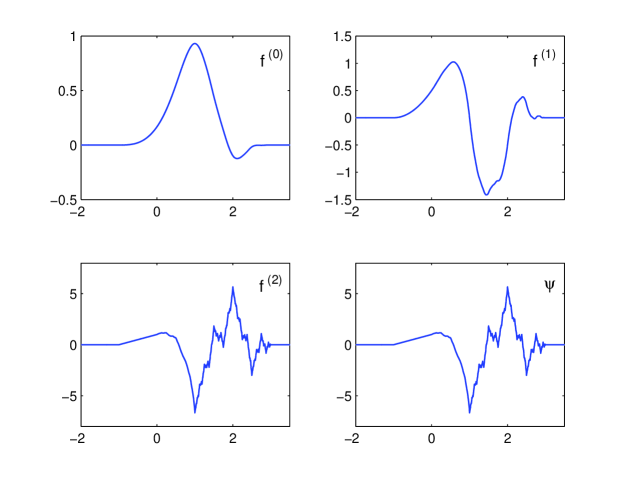
Figure 1: Limit functions for Example 35, showing the three entries of the limit function of the Hermite subdivision scheme and the limit function of the associated convergent difference scheme.

For some time it was conjectured that all $C^{d}$ convergent Hermite subdivision schemes must satisfy a spectral condition. This is disproved by the following example of a family of convergent schemes that satisfies no spectral condition.

Theorem 36

If the nonzero elements of the matrix $\widetilde{\boldsymbol{B}}^{*}$ are of the form

$$\widetilde{b}_{jk}^{*}(z) = (z^{-1}-1)^{j+1}\,h_{jk}^{*}(z),\qquad 0\leq k<j<d,$$

$$\widetilde{b}_{jj}^{*}(z) = \frac{(z^{-1}-1)^{j+1}}{2^{j+1}},\qquad j=0,\dots,d-1,$$

$$\widetilde{b}_{dj}^{*}(z) = \frac{1}{2}(z^{-1}+1)\,\left(z^{-2}-1\right)^{d-j}\qquad j=0,\dots,d,$$

then there exists a $C^{d}$–convergent Hermite subdivision scheme whose mask ${\boldsymbol{A}}$ satisfies $\widetilde{T}_{\Delta}S_{\boldsymbol{A}}=2^{-d}S_{\widetilde{\boldsymbol{B}}}\widetilde{T}_{\Delta}$.

Proof:  Since ${\boldsymbol{B}}$ is lower triangular with contractions on the diagonal, the scheme $S_{\widetilde{B}}$ is contractive. The factorization is satisfied by construction. $\Box$

6.2 A generic construction for arbitrary Taylor operators

For an arbitrary generalized Taylor operator $\widetilde{T}$, we want to construct convergent schemes that factorize with respect to $\widetilde{T}$, thus showing that convergence theory widely exceeds spectral conditions.

Theorem 37

For any $d\in\mathbb{N}$ and any generalized Taylor operator $\widetilde{T}$ of order $d$ there exists a convergent Hermite subdivision scheme with mask ${\boldsymbol{A}}$ that factors with $\widetilde{T}$, that is, such that $\widetilde{T}S_{\boldsymbol{A}}=2^{-d}S_{\widetilde{\boldsymbol{B}}}\widetilde{T}$ for some appropriate $\widetilde{\boldsymbol{B}}$.

The proof continues the construction from the preceding subsection by giving an explicit way to construct the polynomials $h_{dj}^{*}$, $j=0,\dots,d$, in such a way that $S_{\boldsymbol{A}}$ admits the factorization.

Proof:  We will again set

$$\widetilde{b}_{dj}^{*}(z)=(z^{-1}-1)^{d-j}\,h_{dj}^{*}(z^{-1}),\qquad$$ (57)

and make use of (53) and (54) to determine the vectors

$${\boldsymbol{h}}_{j}=\begin{bmatrix}h_{j,j+1}\\ \vdots\\ h_{j1}\end{bmatrix}:=\begin{bmatrix}\left(h_{dj}^{*}\right)^{(j+1)}(1)\\ \vdots\\ \left(h_{dj}^{*}\right)^{\prime}(1)\end{bmatrix}\in\mathbb{R}^{j+1},\qquad j=0,\dots,d-1,$$

which define $\widetilde{\boldsymbol{B}}^{*}$ and eventually the desired mask ${\boldsymbol{A}}^{*}$. We stack these vectors into the column vector

$${\boldsymbol{h}}:=\begin{bmatrix}{\boldsymbol{h}}_{d-1}\\ \vdots\\ {\boldsymbol{h}}_{0}\end{bmatrix}\in\mathbb{R}^{\frac{d(d+1)}{2}}.$$

Again, let $h_{dd}^{*}(z)$ be the symbol of a contractive mask and recall that

$$h_{dj}^{*}(1)=2^{d-j},\qquad j=0,\dots,d,$$ (58)

is necessary due to Lemma 27 to obtain $S_{\boldsymbol{B}}$ as a convergent vector subdivision scheme. Taking (58) into account, the requirement for ${\boldsymbol{h}}_{d-1}$ can be obtained by setting $j=d$ in (51), which yields

$$h_{d-1,r}+\sum_{k=1}^{r-1}w_{d,d-k}\frac{r!}{(r-k)!}h_{d-1-k,r-k}$$

$$= 2\left(h_{dd}^{*}\right)^{(r)}(1)+r\left(h_{dd}^{*}\right)^{(r-1)}(1)-w_{d,d-r}2^{r+1},\qquad r=1,\dots,d-1.$$

In the same way, (52) transforms into

$$h_{d-1,d}+\sum_{k=1}^{d-1}w_{d,d-k}\frac{d!}{(d-k)!}h_{d-1-k,d-k}=2\left(h_{dd}^{*}\right)^{(d)}(1)+d\,\left(h_{dd}^{*}\right)^{(d-1)}(1).$$

In matrix form, this can be rewritten as

$${\boldsymbol{b}}_{d} = \left[\begin{array}[]{cccc|ccc|c|c}1&&&&*&&&\dots&*\\ &\ddots&&&&\ddots&&&0\\ &&1&&&&*&&\vdots\\ &&&1&0&\dots&0&\dots&0\end{array}\right]{\boldsymbol{h}}$$

$$=: \begin{bmatrix}{\boldsymbol{I}}_{d}&-{\boldsymbol{H}}_{d,d-2}&\dots&-{\boldsymbol{H}}_{d,0}\end{bmatrix}{\boldsymbol{h}},$$

where

$${\boldsymbol{H}}_{d,k}=-w_{d,k+1}\,\begin{bmatrix}\frac{d!}{(k+1)!}\\ &\ddots\\ &&\frac{(d-k)!}{1!}\\ 0&\dots&0\\ \vdots&\ddots&\vdots\\ 0&\dots&0\end{bmatrix}\in\mathbb{R}^{d\times k+1},\qquad k=0,\dots,d-2,$$

and

$${\boldsymbol{b}}_{d}:=\begin{bmatrix}2\left(h_{dd}^{*}\right)^{(d)}(1)+d\,\left(h_{dd}^{*}\right)^{(d-1)}(1)\\ 2\left(h_{dd}^{*}\right)^{(d-1)}(1)+(d-1)\left(h_{dd}^{*}\right)^{(d-2)}(1)-2^{d}\,w_{d,1}\\ \vdots\\ 2\left(h_{dd}^{*}\right)^{(1)}(1)+1-4\,w_{d,d-1}\end{bmatrix}\in\mathbb{R}^{d}.$$

The conditions (51) and (52) for $q_{d-1}$ can, in the same way, be written as

$$0=2h_{d-1,d-1}+(d-1)h_{d-1,d-2}-h_{d-2,d-1}-\sum_{k=1}^{d-2}w_{d-1,k}\frac{(d-1)!}{k!}h_{k-1,k},$$

as well as for $r=2,\dots,d-2$,

$$2^{r+2}\,w_{d-1,d-1-r}=2h_{d-1,r}+r\,h_{d-1,r-1}-h_{d-2,r}-\sum_{k=1}^{r-1}w_{d-1,d-1-k}\frac{r!}{(r-k)!}h_{d-2-k,r-k},$$

and finally the case $r=1$

$$2^{d-1}=2h_{d-1,r}-h_{d-2,r}.$$

taking the matrix form

$${\boldsymbol{b}}_{d-1} = \left[\begin{array}[]{ccccc|cccc|c|c}0&2&d-1&&&-1&&&&\dots&*\\ 0&&2&\ddots&&&-1&&&&0\\ \vdots&&&\ddots&2&&&\ddots&&&\vdots\\ 0&&&&2&&&&-1&\dots&0\\ \end{array}\right]{\boldsymbol{a}}$$

$$=: \begin{bmatrix}{\boldsymbol{C}}_{d-1}&-{\boldsymbol{I}}_{d}&{\boldsymbol{H}}_{d-1,d-3}&\dots&{\boldsymbol{H}}_{d-1,0}\end{bmatrix}{\boldsymbol{h}}$$

with

$${\boldsymbol{C}}_{j}:=\begin{bmatrix}0&2&j\\ 0&&2&\ddots\\ \vdots&&&\ddots&2\\ 0&&&&2\\ \end{bmatrix}\in\mathbb{R}^{j},\qquad j=2,\dots,d-1,\qquad{\boldsymbol{C}}_{1}:=\begin{bmatrix}0&2\\ 0&0\\ \end{bmatrix},$$

and

$${\boldsymbol{H}}_{d-1,k}=-w_{d-1,k+1}\begin{bmatrix}\frac{(d-1)!}{(k+1)!}\\ &\ddots\\ &&\frac{(d-1-k)!}{1!}\\ 0&\dots&0\\ \vdots&\ddots&\vdots\\ 0&\dots&0\end{bmatrix}\in\mathbb{R}^{d-1\times k+1},\qquad k=0,\dots,d-3.$$

With the general definition

$${\boldsymbol{H}}_{j,k}=-w_{j,k+1}\begin{bmatrix}\frac{j!}{(k+1)!}\\ &\ddots\\ &&\frac{(j-k)!}{1!}\\ 0&\dots&0\\ \vdots&\ddots&\vdots\\ 0&\dots&0\end{bmatrix}\in\mathbb{R}^{j\times k+1},\qquad k=0,\dots,j-2,\quad j=1,\dots,d,$$ (69)

the conditions (51) and (52) result in the system

$${\boldsymbol{b}}=\begin{bmatrix}{\boldsymbol{b}}_{d}\\ \vdots\\ {\boldsymbol{b}}_{1}\end{bmatrix}=\begin{bmatrix}{\boldsymbol{I}}_{d}&-{\boldsymbol{H}}_{d,d-2}&-{\boldsymbol{H}}_{d,d-3}&\dots&-{\boldsymbol{H}}_{d,0}\\ {\boldsymbol{C}}_{d-1}&-{\boldsymbol{I}}_{d}&{\boldsymbol{H}}_{d-1,d-3}&\dots&{\boldsymbol{H}}_{d-1,0}\\ &\ddots&\ddots&\ddots&\vdots\\ &&{\boldsymbol{C}}_{1}&-1&{\boldsymbol{H}}_{1,0}\end{bmatrix}{\boldsymbol{h}}=:{\boldsymbol{H}}{\boldsymbol{h}}.$$ (70)

By Lemma 39, which we prove next, this linear system has a unique solution ${\boldsymbol{h}}$ for any given polynomial $h_{dd}^{*}(z)$, which, by (57), defines the symbols $\widetilde{b}_{dj}^{*}(z)$, $j=0,\dots,d$, with $\widetilde{b}_{dd}^{*}(z)=h_{dd}^{*}(z)$ and therefore

$$\widetilde{\boldsymbol{B}}^{*}(z)=\begin{bmatrix}\frac{z^{-1}-1}{2}\\ (z^{-1}-1)^{2}\,h_{10}^{*}(z)&\frac{(z^{-1}-1)^{2}}{4}\\ \vdots&\ddots&\ddots\\ (z^{-1}-1)^{d}\,h_{d-1,0}^{*}(z)&\dots&(z^{-1}-1)^{d}\,h_{d-1,d-2}^{*}(z)&\frac{(z^{-1}-1)^{d}}{2^{d}}\\ \widetilde{b}_{d0}^{*}(z)&\dots&\widetilde{b}_{d,d-2}^{*}(z)&\widetilde{b}_{d,d-1}^{*}(z)&\widetilde{b}_{dd}^{*}(z)\end{bmatrix}$$

is the symbol of a contractive scheme that satisfies the conditions from Lemma 27 and for which there exists a mask ${\boldsymbol{A}}$ such that $\widetilde{S}_{\boldsymbol{A}}=S_{\widetilde{\boldsymbol{B}}}\widetilde{T}$. Therefore, ${\boldsymbol{A}}$ defines a $C^{d}$–convergent Hermite subdivision scheme. $\Box$

Remark 38

Recall that the whole construction process only had the purpose of finding the last row of the lower triangular symbol $\widetilde{B}^{*}(z)$. All other entries could be chosen in a straightforward way.

Lemma 39

Matrix ${\boldsymbol{H}}$ from (70) satisfies $|\det{\boldsymbol{H}}|=1$.

Proof:  Since the first column of ${\boldsymbol{C}}_{d-1}$ is zero, we can start with an expansion with respect to the first column, yielding that $\det{\boldsymbol{H}}$ is the same as the determinant of ${\boldsymbol{A}}$ with first row and column erased. Then, we note that the last row of the matrix in (6.2) has only one nonzero entry, namely $-1$. Expansion with respect to this row also removes the column that contains the $2$ in the last row of (70). Expanding with respect to this row then removes the row that contains the last nonzero element in ${\boldsymbol{H}}_{d,d-2}$ in (6.2), so that we can now expand with respect to the second last row of (6.2). Circling in this way, we expand the determinant by means of factors that are $\pm 1$, hence, the determinant of ${\boldsymbol{H}}$ is $\pm 1$ and in particular independent of $\widetilde{T}$, that is, independent of ${\boldsymbol{w}}_{1},\dots,{\boldsymbol{w}}_{d}$. $\Box$

7 Examples

To illustrate the potential of the methods, we start with two examples of masks obtained by the construction process in Theorem 37. We restrict ourselves to the simplest nontrivial case $d=2$ here.

Example 40

One parameter, $w_{21}$, can be chosen freely. The associated linear system for ${\boldsymbol{h}}$ becomes

$$\begin{bmatrix}1&&2w_{21}\\ &1&\\ &2&-1\end{bmatrix}\begin{bmatrix}h_{12}\\ h_{11}\\ h_{01}\end{bmatrix}=\begin{bmatrix}2\left(h_{dd}^{*}\right)^{\prime\prime}(1)+2\left(h_{dd}^{*}\right)^{\prime}(1)\\ 2\left(h_{dd}^{*}\right)^{\prime}(1)+1-4w_{21}\\ 2\end{bmatrix}$$

which gives

$$h_{11} = 2\left(h_{dd}^{*}\right)^{\prime}(1)+1-4w_{21}$$

$$h_{01} = 2a_{11}-2=4\left(h_{dd}^{*}\right)^{\prime}(1)-8w_{21}$$

$$h_{12} = 2\left(h_{dd}^{*}\right)^{\prime\prime}(1)+2\left(h_{dd}^{*}\right)^{\prime}(1)-2w_{21}a_{01}$$

$$= 2\left(\left(h_{dd}^{*}\right)^{\prime\prime}(1)+\left(h_{dd}^{*}\right)^{\prime}(1)\left(1-4w_{21}\right)+8w_{21}^{2}\right).$$

Using the simplest possible choice $h_{dd}^{*}(z)=\frac{1}{2}(z+1)$, we get

$$h_{12} = 1-4w_{21}+16w_{21}^{2}$$

$$h_{11} = 2-4w_{21}$$

$$h_{01} = 2-8w_{21},$$

and therefore

$$h_{21}^{*}(z) = \frac{\left((1-4w_{21})z+(1+4w_{21})\right)^{2}}{2}+2w_{21}(z^{2}-1)$$

$$h_{20}^{*}(z) = 4+(2-8w_{21})(z-1)=2\left((1-4w_{21})z+(1+4w_{21})\right),$$

yielding

$$\widetilde{b}_{22}^{*}(z) = \frac{1}{2}(z^{-1}+1)$$

$$\widetilde{b}_{21}^{*}(z) = (1-4w_{21}+8w_{21}^{2})z^{-3}+8w_{21}(1-3w_{21})z^{-2}-(1+4w_{21}-24w_{21}^{2})z^{-1}-8w_{21}^{2}$$

$$\widetilde{b}_{20}^{*}(z) = (4-8w_{21})z^{-2}-(4-16w_{21})z^{-1}+8w_{21}^{2}.$$

The resulting limit functions are plotted in Fig 2.

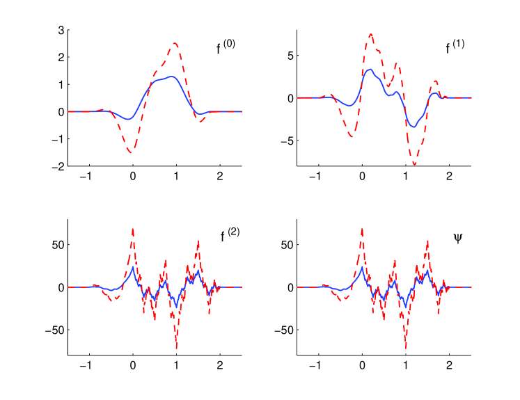
Figure 2: Limit functions for the constructions of Example 40 for the values $w_{21}=\frac{1}{2}$ (blue, solid) and $w_{21}=1$ (red, dashed).

Example 41

In continuation of Example 40, we now choose an arbitrary contractive version based on

$$h_{dd}^{*}(z)=\frac{(z+1)^{n}}{2^{n}}$$

which has the property that

$$h_{dd}^{*}(1)=1,\qquad\left(h_{dd}^{*}\right)^{\prime}(1)=\frac{n}{2},\qquad\left(h_{dd}^{*}\right)^{\prime\prime}(1)=\frac{n(n-1)}{4},$$

so that

$$h_{12} = 2\left(\frac{n(n-1)}{4}+\frac{n}{2}\,(1-4\,w_{21})+8w_{21}^{2}\right)=\frac{n(n+1)}{2}-4nw_{21}+16w_{21}^{2},$$

$$h_{11} = n+1-4w_{21}$$

$$h_{01} = 2n-8w_{21},$$

which leads to the graphs shown in Fig. 3. This even gives a whole family of convergent schemes with the additional parameter $n$.

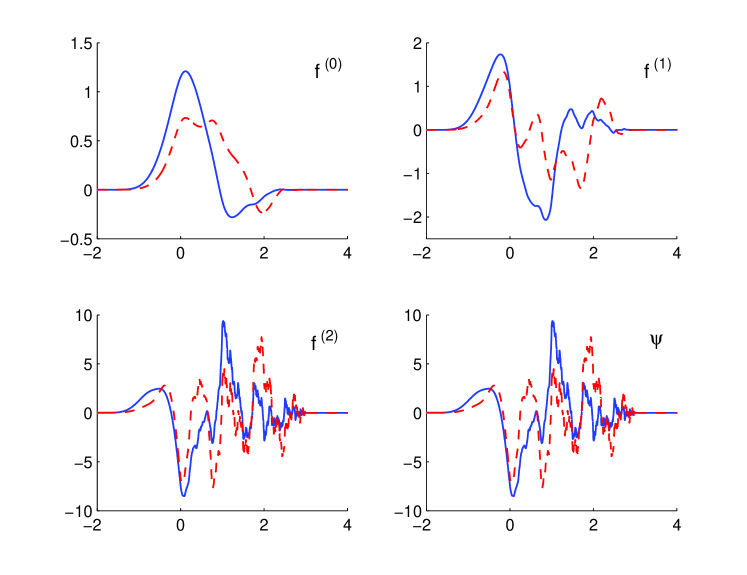
Figure 3: Limit functions for Example 41 for the values $w_{21}=\frac{1}{2}$ (blue, solid) and $w_{21}=1$ (red, dashed) and $n=5$.

The last example revisits a Hermite subdivision scheme based on B–splines that was introduced in [14] and further studied in [16] as one of the first examples of a family of convergent Hermite subdivision schemes that do not satisfy the spectral condition.

This scheme is based on a construction detailed by Micchelli in [17]. Let $\varphi_{0}(x)=\chi_{[0,1]}$ and define, for $r=1,2,\ldots$, the cardinal B–spline $\varphi_{r}=\varphi_{0}*\varphi_{r-1}$. We recall that $\varphi_{r}$ is a $C^{r-1}$ piecewise polynomial of degree $r$ with support $[0,r+1]$ that satisfies the refinement equation

$$\varphi_{r}(x)=\frac{1}{2^{r}}\sum_{\alpha\in\mathbb{Z}}\begin{pmatrix}r+1\\ \alpha\end{pmatrix}\varphi_{r}(2x-\alpha),\qquad\begin{pmatrix}i\\ j\end{pmatrix}=\left\{\begin{array}[]{ccl}\frac{i!}{j!(i-j)!}&&\text{ if }0\leq j\leq i,\\ 0&&\text{otherwise}.\end{array}\right.$$

The function $v(x)=\sum_{\alpha\in\mathbb{Z}}f^{(0)}_{0}(\alpha)\varphi_{r}(x-\alpha)$ can be written as $v(x)=\sum_{\alpha\in\mathbb{Z}}f^{(0)}_{n}(\alpha)\varphi_{r}\left(2^{n}\,x-\alpha\right)$, $n\in\mathbb{N}_{0}$, where

$$f^{(0)}_{n+1}(\cdot)=\sum_{\beta\in\mathbb{Z}}a_{r}(\cdot-2\beta)f^{(0)}_{n}(\beta),\qquad a_{r}(\alpha)=\frac{1}{2^{r}}{r+1\choose\alpha},\qquad\alpha\in\mathbb{Z}.$$ (71)

We have proved in [16, Proposition 5.3] that for $i=0,\ldots,r$ one has

$$S_{a_{r}}p_{i}=\frac{1}{2^{i}}p_{i},\qquad p_{i}:=\ell_{r}^{(r-i)},\qquad\ell_{r}(x):=\frac{1}{r!}\prod_{j=1}^{r}(x+j).$$ (72)

Taking derivatives of $v$,

$$\dfrac{d^{i}v}{dx^{i}}(x)=\sum_{\alpha\in\mathbb{Z}}2^{ni}\Delta^{i}f^{(0)}_{n}(\alpha-i)\,\varphi_{r-i}\left(2^{n}x-\alpha\right),\qquad i=0,\dots,r-1,$$

we define Hermite subdivision schemes of degree $d\leq r$ with mask ${\boldsymbol{A}}(\alpha)$ and support $[0,r+d+1]$ by applying differences to the mask $a_{r}$, yielding the following observation.

Example 42

The Hermite subdivision scheme based on

$${\boldsymbol{A}}(\alpha)=\begin{bmatrix}a_{r}(\alpha)&0&\ldots&0\\ \Delta a_{r}(\alpha-1)&0&\ldots&0\\ \Delta^{2}a_{r}(\alpha-2)&0&\ldots&0\\ \vdots\\ \Delta^{d}a_{r}(\alpha-d)&0&\ldots&0\end{bmatrix},\qquad{\boldsymbol{A}}^{*}(z)=\frac{(1+z)^{r+1}}{2^{r}}\begin{bmatrix}1&0&\ldots&0\\ (1-z)&0&\ldots&0\\ (1-z)^{2}&0&\ldots&0\\ \vdots\\ (1-z)^{d}&0&\ldots&0\end{bmatrix}.$$

has as limit function the vector consisting of the B–spline and its derivatives but does not satisfy the classical spectral condition, see [14].

In the following, we prove that the Hermite scheme from Example 42 possesses a spectral chain.

Firstly, the computation of Taylor expansions yields that there for $p\in\Pi_{d}$ the vectors ${\boldsymbol{v}}_{p}=[p,p^{\prime},\ldots,p^{(d)}]^{T}$ and $\hat{\boldsymbol{v}}_{p}=[p,\Delta p(\cdot-1),\ldots,\Delta^{d}p(\cdot-d)]^{T}$ satisfy

$$\hat{\boldsymbol{v}}_{p}={\boldsymbol{R}}{\boldsymbol{v}}_{p},\qquad{\boldsymbol{R}}:=\begin{bmatrix}1&0&0&\ldots&0\\ &1&*&\dots&*\\ &&\ddots&\ddots&\vdots\\ &&&1&*\\ &&&&1\end{bmatrix}\in\mathbb{R}^{(d+1)\times(d+1)},$$

where the $d-j$-th last components of $\hat{\boldsymbol{v}}_{p}$ are zero if $p\in\Pi_{j}$, $j<d$.

Secondly, (72) yields $S_{a_{r}}p_{j}=2^{-j}p_{j}$ and the first component of ${\boldsymbol{v}}_{p_{j}}$ is $p_{j}$ , since the only non zero column of the matrices ${\boldsymbol{A}}(\alpha)$ is the first one, we therefore deduce that

$$S_{{\boldsymbol{A}}}{\boldsymbol{v}}_{p_{j}}=S_{{\boldsymbol{A}}}\begin{bmatrix}p_{j}\\ *\end{bmatrix}=S_{{\boldsymbol{A}}}\hat{\boldsymbol{v}}_{p_{j}}=\frac{1}{2^{j}}\hat{\boldsymbol{v}}_{p_{j}},\qquad j=0,\dots,d,$$

so that for $j=0,\ldots,d$, the vectors $\hat{\boldsymbol{v}}_{j}=\hat{\boldsymbol{v}}_{p_{j}}$ satisfy the spectral condition. To show that the associated $\hat{\boldsymbol{v}}_{j}$ form a chain, we have to find the appropriate generalized Taylor operator annihilating $\hat{\boldsymbol{v}}_{d}$, its uniqueness being guaranteed by Corollary 8. This operator is $\widetilde{T}_{S,d}$ from (20) in Example 16. Indeed, by Lemma 44 proved at the end of this section,

$$\left(\widetilde{T}_{S,d}{\boldsymbol{v}}_{d}\right)_{d-j} = \Delta\left(\Delta^{j}p_{d}(\cdot-j)\right)-\sum_{k=1}^{d-j}\Delta^{k}\left(\Delta^{j}p_{d}(\cdot-j)\right)(\cdot-k)$$

$$= \Delta^{d}p_{d}(\cdot-j-d+1)-\Delta^{d}p_{d}(\cdot-j-d)=0,\qquad j=0,\dots,d,$$

since $\Delta^{d}p_{d}=1$. The same argument also shows that $\widetilde{T}_{S,d}\hat{\boldsymbol{v}}_{j}=0$, $j=0,\dots,d-1$. Therefore ${\boldsymbol{V}}$ forms a spectral chain for $S_{\boldsymbol{A}}$ and by Theorem 24 there exists a finite mask ${\boldsymbol{B}}\in\ell^{(d+1)\times(d+1)}(\mathbb{Z})$ such that $\widetilde{T}_{S,d}\,S_{\boldsymbol{A}}=S_{\widetilde{\boldsymbol{B}}}\,\widetilde{T}_{S,d}$.

Example 43 (Example 42 continued)

For $r=4$, $d=3$, we obtain

$$\tilde{\boldsymbol{B}}^{*}(z)=\begin{bmatrix}-{{\left(z-1\right)^{3}\,z\,\left(1+z\right)^{4}}\over{2}}&{{\left(z-1\right)^{2}\,z^{3}\,\left(1+z\right)^{3}}\over{2}}&-{{\left(z-1\right)\,z^{3}\,\left(1+z\right)^{2}}\over{2}}&{{z^{3}\,\left(1+z\right)}\over{2}}\\[2.84526pt] -{{\left(z-1\right)^{3}\,z\,\left(1+z\right)^{4}}\over{2}}&{{\left(z-1\right)^{2}\,z^{3}\,\left(1+z\right)^{3}}\over{2}}&-{{\left(z-1\right)\,z^{3}\,\left(1+z\right)^{2}}\over{2}}&{{z^{3}\,\left(1+z\right)}\over{2}}\\[2.84526pt] -{{\left(z-1\right)^{3}\,z\,\left(1+z\right)^{4}}\over{2}}&{{\left(z-1\right)^{2}\,z^{3}\,\left(1+z\right)^{3}}\over{2}}&-{{\left(z-1\right)\,z^{3}\,\left(1+z\right)^{2}}\over{2}}&{{z^{3}\,\left(1+z\right)}\over{2}}\\[2.84526pt] -{{\left(z-1\right)^{3}\,z\,\left(1+z\right)^{4}}\over{2}}&{{\left(z-1\right)^{2}\,z^{3}\,\left(1+z\right)^{3}}\over{2}}&-{{\left(z-1\right)\,z^{3}\,\left(1+z\right)^{2}}\over{2}}&{{z^{3}\,\left(1+z\right)}\over{2}}\\ \end{bmatrix}.$$

We close the paper with a simple identity on forward and backward differences needed for Example 43 that may, however, be of independent interest.

Lemma 44

For $p\in\Pi$ and $n\in\mathbb{N}$ we have that

$$\Delta p=\sum_{k=1}^{n-1}\Delta^{k}p(\cdot-k)+\Delta^{n}p(\cdot-n+1).$$ (73)

Proof:  Expanding the differences as

$$\Delta^{k}p(\cdot-k)=\sum_{j=0}^{k}(-1)^{j}{k\choose j}p(\cdot-j),$$

we find that

$$\Delta^{n}p(\cdot-n+1)+\sum_{k=1}^{n-1}\Delta^{k}p(\cdot-k)$$

$$= p(\cdot+1)+\sum_{j=0}^{n-1}(-1)^{j+1}{n\choose j+1}p(\cdot-j)+\sum_{k=1}^{n-1}\sum_{j=0}^{k}(-1)^{j}{k\choose j}p(\cdot-j)$$

$$= p(\cdot+1)-p(\cdot)+\sum_{j=0}^{n-1}(-1)^{j}p(\cdot-j)\left({n\choose j+1}-\sum_{k=j}^{n-1}{k\choose j}\right),$$

from which the claim follows by taking into account the combinatorial identity

$${n\choose j+1}=\sum_{k=j}^{n-1}{k\choose j},\qquad 0\leq j\leq n-1,$$ (74)

which is easily proved by induction on $n$: calling the left hand side of (74) $f(n)$ and the right hand side $g(n)$, the initial step $f(j+1)=g(j+1)=1$ is obvious, while

$$f(n+1)-f(n)={n+1\choose j+1}-{n\choose j+1}={n\choose j}=g(n+1)-g(n)$$

advances the induction. $\Box$

References

[1] A. S. Cavaretta, W. Dahmen, and C. A. Micchelli,
Stationary Subdivision, Mem. Amer. Math. Soc. 453 (1991).
[2]
C. Conti, L. Romani and J. Yoon, Approximation order and
approximate sum rules in subdivision, J. Approx. Theory
207 (2016), 380–401.
565–582.
[3]
C. Conti, M. Cotronei, T. Sauer,
Factorization of Hermite subdivision operators preserving
exponentials and polynomials, Adv. Comput. Math. 45
(2017), 1055–1079.
[4]
C. Conti, M. Cotronei and T. Sauer, Convergence of
level-dependent Hermite subdivision schemes,
Appl. Numer. Math 116 (2017), 119–128.
[5]
M. Cotronei and N. Sissouno, A note on Hermite multiwavelets
with polynomial and exponential vanishing moments,
Appl. Numer. Math 120 (2017), 21–34.
[6]
S. Dubuc and J.-L. Merrien, Hermite subdivision schemes and Taylor
polynomials, Constr. Approx. 29 (2009), 219–245.
[7]
N. Dyn, D. Levin, Analysis of Hermite-type subdivision schemes,
(C. K. Chui and L.L. Schumaker Eds.), Approximation Theory VIII. Vol
2: Wavelets and Multilevel Approximation (College Station, TX,
1995). World Sci., River Edge, NJ, 1995, pp. 117-124.
[8]
N. Dyn and D. Levin, Subdivision schemes in geometric modelling, Acta
Numerica 11 (2002), 73–144.
[9]
B. Han, Vector cascade algorithms and refinable functions in Sobolev
spaces, J. Approx. Theory 124 (2003), 44–88.
[10]
B. Han, M. L. Overton and Th. P. Y. Yu, Design of