Vapor-liquid equilibrium and equation of state of two-dimensional fluids from a discrete perturbation theory

Abstract

The interest in the description of the properties of fluids of restricted dimensionality is growing for theoretical and practical reasons. In this work, we have firstly developed an analytical expression for the Helmholtz free energy of the two-dimensional square-well fluid in the Barker–Henderson framework. This equation of state is based on an approximate analytical radial distribution function for $d$-dimensional hard-sphere fluids (1$\leq d\leq$3) and is validated against existing and new simulation results. The so-obtained equation of state is implemented in a discrete perturbation theory able to account for general potential shapes. The prototypical Lennard-Jones and Yukawa fluids are tested in its two-dimensional version against available and new simulation data with semiquantitative agreement.

I Introduction

The holy grail in the theory of liquids is perhaps the development and application, from a purely molecular perspective, of equations of state (EoSs).Hansen and McDonald (2006); Solana (2013); Santos (2016) This interplay between molecular theories of fluids and experiments with practical applications was born in the early work of van der Waals.Rowlinson (1979)

Statistical mechanics perturbation theories (PTs) for molecular or atomic fluidsBarker and Henderson (1967a); Barker and Henderson (1967b); Chandler and Weeks (1970); Henderson and Barker (1970); Weeks et al. (1971); Zhou and Solana (2009); Solana (2013) are of pivotal importance and constitute a handable tool for the applied sciences, given their negligible computational cost in comparison with simulations and the mathematical simplicity and intuitivity in comparison with integral equations or density functional theory. Since for isotropic fluids the structure is led by the repulsive part of the global interaction, PTs are based on a decoupling of the total intermolecular potential in perturbative and reference contributions. The reference part accounts for the structure correlation functions of the fluid and consequently it is desirable to know it analytically. Hence, for some simple two-dimensional (2D) models and their mixtures, the hard-disk (HD) model emerges as the most common candidate for being used as reference in PT. Very often, the perturbative contribution contains the pairwise atomic interaction describing the so-called van der Waals forces. When electrostatic forces are negligible and the fluid is of atomic character, the functionality of the potential energy surface becomes only dependent on the intermolecular distance. This is the case of many emblematic potential models, such as the widely studied hard-sphere, square-well (SW), Yukawa, Lennard-Jones (LJ), and their 2D counterparts.Phillips et al. (1981); Reddy and O’Shea (1986); Rovere et al. (1990); Löwen (1992); Mulero et al. (1999); Ouyang et al. (2011); Khordad (2012); Murillo and Gericke (2003); Lang et al. (2014); Vaulina and Koss (2014); Kryuchkov et al. (2017) Although an extensive work on three-dimensional (3D) systems can be found,Zhou and Solana (2009) few works on the application of PTs to 2D models have been reported in the literature.Mishra and Sinha (1984); Henderson (1977) For instance, the statistical associating fluid theory of variable range (SAFT-VR) in its 2D version has been applied to predict the adsorption isotherms of pure fluids and mixtures onto different kinds of surfaces.Buenrostro-González et al. (2004); Martínez et al. (2007); Jiménez-Serratos et al. (2008); Castro et al. (2009); Trejos et al. (2014); Martínez et al. (2017); Castro et al. (2011); Castro and Martínez (2013); Trejos et al. (2018)

Another route is the discrete PT (DPT). From theoretical grounds, the Zwanzig PT (later popularized by Barker and HendersonBarker and Henderson (1967a); Barker and Henderson (1967b)) is the basis for the development of the DPTBenavides and Gil-Villegas (1999) for atomic models Chapela et al. (2010) and its extension to polarBenavides and Gámez (2011) and molecular fluidsGámez and Benavides (2013); Gámez (2014) constitute a powerful alternative to traditional PTs. It has been established as a versatile generator of EoSs that are analytical in terms of density, temperature, and intermolecular parameters characterizing the interaction, so that all thermodynamic properties can be easily obtained using common thermodynamic relations. Although, by construction, these theories use the hard-sphere model as a reference potential, they also provide good approximations for the thermodynamic properties of soft-core potentials, as is the case of the LJ or Kihara fluids. Very recently, the situation has been partly circumvented with the implementation of a temperature-dependent Barker–Henderson (BH) diameterCervantes et al. (2015) for the hard-core wall taking into account the repulsive van der Waals volume. Hence, in general, the DPT can be applied to any intermolecular potential model that can be expressed as the sum of a sequence of square-shoulder (SS) and SW steps. The strategy followed in the present work is to incorporate the approximate analytical radial distribution function (RDF) for 2D fluids described in Refs. Yuste and Santos, 1993; Santos and López de Haro, 2016 into a BH high-temperature expansion for the SW2D model. The improvement over the existing EoS for SW2D fluids motivated us to integrate this new EoS in a general DPT able to describe arbitrary potential functions. Both the 2D LJ and Yuwaka potentials of variable range are considered as benchmark examples.

This paper is organized as follows. In Sec. II a description of the BH PT for SW2D fluids is presented. A possible parameterization of the so-obtained EoS is also included for practical reasons. A short review of the DPT procedure to map a continuous potential onto a sequence of discrete steps is also incorporated in Sec. II, together with a description of our Gibbs ensemble Monte Carlo (GEMC) simulation results. Illustrative examples of the applicability of our treatment are given in Sec. III. Finally, we close the paper with Sec. IV, where the main conclusions and perspectives of this work are presented.

II Theoretical framework

II.1 Perturbation theory for two-dimensional square-well fluids

In the framework of the BH PT,Barker and Henderson (1967a); Barker and Henderson (1967b) the pair potential, $u(r)$, is decomposed into two contributions,

$$u(r)=u^{\text{HD}}(r)+w(r),$$ (1)

where $u^{\text{HD}}(r)$ and $w(r)$ are the repulsive HD and (attractive) perturbation pair potential interactions, respectively. The HD contribution is given by

$$u^{\text{HD}}(r)=\begin{cases}\infty,&r<\sigma,\\ 0,&r\geq\sigma,\end{cases}$$ (2)

where $r$ is the distance between centers of two particles and $\sigma$ is the hard-core diameter. For a system of particles of diameter $\sigma$ interacting via a SW pair potential, the perturbation contribution is given by

$$w^{\text{SW}}(r)=\begin{cases}0,&r<\sigma,\\ \varepsilon,&\sigma\leq r<\lambda\sigma,\\ 0,&r\geq\lambda\sigma,\end{cases}$$ (3)

where $-\varepsilon>0$ and $\lambda\sigma$ are the depth and range of the SW potential, respectively. If $\varepsilon>0$, Eq. (3) describes as well the case of a (repulsive) SS interaction potential

Once the pair potential is split as described above, the corresponding Helmholtz free energy per particle, $a$, for a general 2D fluid can be written in the BH approach asBarker and Henderson (1967a); Barker and Henderson (1967b)

$${a}={a^{\text{id}}}+{a_{\text{ex}}^{\text{HD}}}+\beta{a_{1}}+\beta^{2}{a_{2}},$$ (4)

where $\beta=1/kT$ ($k$ and $T$ being the Boltzmann constant and the temperature, respectively), $a^{\text{id}}$ is the Helmholtz free energy of a 2D ideal gas, $a_{\text{ex}}^{\text{HD}}$ is the excess Helmholtz free energy of the reference HD fluid, and $a_{1}$, $a_{2}$ are the first- and second-order perturbation terms, respectively.Barker and Henderson (1967a) The ideal gas contribution is given by

$$\beta{a^{\text{id}}}=\ln(\rho\lambda_{B}^{2})-1,$$ (5)

where $\lambda_{B}$ is the de Broglie wavelength and $\rho$ is the number of particles per unit area. According to the accurate EoS for HDs proposed by Henderson,Henderson (1975)

$$\beta{a_{\text{ex}}^{\text{HD}}}=\frac{9}{8}\frac{\eta}{(1-\eta)}-\frac{7}{8}\ln(1-\eta),$$ (6)

where $\eta=\pi\rho\sigma^{2}/4$ is the 2D packing fraction.

The first-order contribution to the Helmholtz free energy, $a_{1}$, can be written as

$$\beta{a_{1}}=\pi\rho\int_{\sigma}^{\infty}dr\,w(r)r{g}^{\text{HD}}(r),$$ (7)

where $g^{\text{HD}}(r)$ is the RDF of the HD fluid. The second-order perturbation term is given in the so-called “local compressibility” approximation by

$$\beta{a_{2}}=-\frac{\pi}{2}K^{\text{HD}}\rho\frac{\partial}{\partial\rho}\left[\rho\int_{\sigma}^{\infty}dr\,w^{2}(r)r{g}^{\text{HD}}(r)\right],$$ (8)

where $K^{\text{HD}}=kT(\partial\rho/\partial P^{\text{HD}})_{T}$ is the (reduced) isothermal compressibility of the HD fluid, which is given by

$$K^{\text{HD}}(\eta)=\frac{(1-\eta)^{3}}{1+\eta+\frac{3}{8}\eta^{2}-\frac{1}{8}\eta^{3}},$$ (9)

according to the Henderson EoS.Henderson (1975)

Equations (7) and (8) apply to any perturbation contribution $w(r)$. In the special case of the SW interaction, Eq. (3), the perturbation terms $a_{1}$ and $a_{2}$ can be rewritten as

$$\beta a_{1}^{\text{SW}}=\varepsilon a_{1}^{*},\quad\beta a_{2}^{\text{SW}}=\varepsilon^{2}a_{2}^{*},$$ (10a)

$$a_{1}^{*}(\eta,\lambda)=4\eta J(\eta,\lambda),$$ (10b)

$$a_{2}^{*}(\eta,\lambda)=-\frac{1}{2}K^{\text{HD}}(\eta)\eta\frac{\partial a_{1}^{*}(\eta,\lambda)}{\partial\eta},$$ (10c)

where we have introduced the dimensionless quantity

$$J(\eta,\lambda)\equiv\sigma^{-2}\int_{\sigma}^{\lambda\sigma}dr\,r{g}^{\text{HD}}(r,\eta).$$ (11)

The integral (11) requires the prior knowledge of the RDF for a HD fluid. Obviously, it is highly desirable to have an analytical approximation for ${g}^{\text{HD}}(r)$, thermodynamically consistent with the Henderson EoS, in such a way that the integral $J(\eta,\lambda)$ can be obtained for arbitrary values of both $\eta$ and $\lambda$. This would allow, by insertion of Eqs. (5), (6), and (10) into Eq. (4), to determine the free energy as an explicit function of density, temperature, and the two parameters ($\varepsilon$ and $\lambda$) characterizing the SW potential. Here, we will make use of the approximation for ${g}^{\text{HD}}(r)$ proposed in Ref. Yuste and Santos, 1993, and recently generalized to any dimensionality $1\leq d\leq 3$,Santos and López de Haro (2016) to obtain $J(\eta,\lambda)$ analytically. The details are presented in the Appendix.

II.2 Effective packing fraction and its parameterization

Following the methodology used for 3D and 2D fluids,Gil-Villegas et al. (1997); Patel et al. (2005); Jiménez-Serratos et al. (2008) one can apply the mean-value theorem to express the integral (11) as

$$J(\eta,\lambda)=g^{\text{HD}}(\xi,\eta)\frac{\lambda^{2}-1}{2},$$ (12)

where $\xi(\eta,\lambda)$ is a certain appropriate distance. As discussed in Gil-Villegas et al.,Gil-Villegas et al. (1997) one can define an effective packing fraction $\eta_{\text{eff}}(\eta,\lambda)$ such that

$$g^{\text{HD}}(\xi,\eta)=g_{\text{cont}}^{\text{HD}}(\eta_{\text{eff}}),$$ (13)

where $g_{\text{cont}}^{\text{HD}}(\eta)$ is the RDF at contact. Its expression consistent with the Henderson EoSHenderson (1975) is

$$g_{\text{cont}}^{\text{HD}}(\eta)=\frac{1-7\eta/16}{(1-\eta)^{2}}.$$ (14)

Combination of Eqs. (12)–(14) yields a quadratic equation for $\eta_{\text{eff}}$ whose physical solution is

$$\eta_{\text{eff}}(\eta,\lambda)=1-\frac{1+\sqrt{1+18Q(\eta,\lambda)/7}}{Q(\eta,\lambda)},$$ (15)

where $Q(\eta,\lambda)\equiv\frac{64}{7}J(\eta,\lambda)/(\lambda^{2}-1)$. Therefore, Eq. (10b) can be rewritten as

$$\beta a_{1}^{*}(\eta,\lambda)=2(\lambda^{2}-1)\eta g_{\text{cont}}^{\text{HD}}(\eta_{\text{eff}}(\eta,\lambda)).$$ (16)

Following Patel et al.,Patel et al. (2005) we have obtained a parameterization for $\eta_{\text{eff}}$ (by taking numerical results for $8\times 10^{-4}\leq\eta\leq 0.63$ and $1.02\leq\lambda\leq 12$) in the form

$$\eta_{\text{eff}}(\eta,\lambda)=\eta\frac{c_{1}(\lambda)+c_{2}(\lambda)\eta}{[1+c_{3}(\lambda)\eta]^{3}},$$ (17)

where the coefficients $c_{1,2,3}$ are given in matrix form by

$$\left(\begin{aligned} c_{1}\\ c_{2}\\ c_{3}\\ \end{aligned}\right)= \begin{pmatrix}0.15605&-0.60341&4.10347&-2.33312\\ -0.82505&12.03157&-40.40351&33.23906\\ 9.73879&-47.09168&66.35256&-28.17232\\ \end{pmatrix}$$

$$\cdot\begin{pmatrix}1/\lambda\\ 1/\lambda^{2}\\ 1/\lambda^{3}\\ 1/\lambda^{4}\\ \end{pmatrix}.$$ (18)

Use of the (approximate) parameterization (17) in Eq. (16), together with Eq. (10c), provides manageable analytical expressions for $a_{1}^{*}$ and $a_{2}^{*}$ that are convenient from the point of view of practical applications.

II.3 Discrete perturbation theory

As commented above, the DPT is a BH PT capable of generating EoSs analytical in the parameters that characterize the intermolecular interactions.Benavides and Gil-Villegas (1999) It can be applied to a great variety of intermolecular potential models that can be discretized as the sum of $p$ steps of SS and SW potentials of variable energy scale $\{\varepsilon_{i}\}$ and width $\{\lambda_{i}\}$. The construction of the DPT is based on the use of the hard-core model as reference potential, what results in a good approximations for the thermodynamic properties of low-density properties of soft-core potentials (such as the LJ fluid) but fails in the prediction of the high and intermediate part of the phase diagram (see, for example, the 3D LJ case treated in Refs. Benavides and Gámez, 2011; Chapela et al., 2010).

A $p$-step discrete potential has the form

$$u^{\text{dis}}(r)=\begin{cases}\infty,&r<\sigma,\\ \varepsilon_{1},&\sigma<r<\lambda_{1}\sigma,\\ \varepsilon_{2},&\lambda_{1}\sigma<r<\lambda_{2}\sigma,\\ \vdots&\vdots\\ \varepsilon_{p},&\lambda_{p-1}\sigma<r<\lambda_{p}\sigma,\\ 0,&r>\lambda_{p}.\end{cases}$$ (19)

If $u^{\text{dis}}(r)$ is intended to represent a given continuous potential $u(r)$, it is convenient to choose

$$\varepsilon_{i}=u\left(\sigma\frac{\lambda_{i-1}+\lambda_{i}}{2}\right),\quad\lambda_{0}=1,$$ (20a)

$$\lambda_{i}=1+i\Delta\lambda,\quad\Delta\lambda=\frac{\lambda_{p}-1}{p}.$$ (20b)

By using the notation $u^{\text{SW}}(r;\varepsilon,\lambda)$ for the SW perturbation function (3), the perturbation contribution to $u^{\text{dis}}(r)$ can be written asBenavides and Gil-Villegas (1999)

$$w^{\text{dis}}(r)=\sum_{i=1}^{p}\left[w^{\text{SW}}(r;\varepsilon_{i},\lambda_{i})-w^{\text{SW}}(r;\varepsilon_{i},\lambda_{i-1})\right].$$ (21)

A similar expression holds for $[w^{\text{dis}}(r)]^{2}$. As a consequence, from Eqs. (7) and (8), one obtains the following forms for the first- and second-order contributions of the free energy corresponding to the potential (19):

$$\beta a_{1}^{\text{dis}}=\sum_{i=1}^{p}\varepsilon_{i}\left[a_{1}^{*}(\eta,\lambda_{i})-a_{1}^{*}(\eta,\lambda_{i-1})\right],$$ (22a)

$$\beta a_{2}^{\text{dis}}=\sum_{i=1}^{p}\varepsilon_{i}^{2}\left[a_{2}^{*}(\eta,\lambda_{i})-a_{2}^{*}(\eta,\lambda_{i-1})\right],$$ (22b)

where, in the 2D case, $a_{1}^{*}(\eta,\lambda)$ and $a_{2}^{*}(\eta,\lambda)$ are given by Eqs. (10b) and (10c), respectively. In summary, the Helmholtz free energy per particle corresponding to the interaction potential (19) is

$$\beta a^{\text{dis}}= \beta a^{\text{id}}+\beta a^{\text{HD}}+\sum_{i=1}^{p}\beta\varepsilon_{i}\left[a_{1}^{*}(\eta,\lambda_{i})-a_{1}^{*}(\eta,\lambda_{i-1})\right]$$

$$+\sum_{i=1}^{p}(\beta\varepsilon_{i})^{2}\left[a_{2}^{*}(\eta,\lambda_{i})-a_{2}^{*}(\eta,\lambda_{i-1})\right].$$ (23)

Once the Helmholtz free energy is known as a function of density, temperature, and the set of potential parameters, the pressure ($P$) and chemical potential ($\mu$) can be obtained by standard thermodynamic relations as

$$Z\equiv\frac{P}{\rho kT}=\rho\frac{\partial\beta a}{\partial\rho},\quad\beta\mu=\beta a+Z.$$ (24)

The vapor-liquid phase boundaries are obtained by solving the nonlinear set of equations that establish the conditions of thermal, mechanical, and chemical equilibrium. Those conditions will be fulfilled by equating the temperature ($T^{v}=T^{l}$), the pressure ($P^{v}=P^{l}$), and the chemical potential ($\mu^{v}=\mu^{l}$) of both vapor ($v$) and liquid ($l$) phases.

II.4 Gibbs ensemble Monte Carlo simulations

In this work, we studied the vapor-liquid phase coexistence of SW2D and LJ2D fluids by using the GEMC simulation method proposed by Panagiotopolous.Panagiotopoulos (1987) We initially placed $N=1152$ particles uniformly distributed in two boxes with equal areas and number of particles $N_{1}=N_{2}=576$ with $N=N_{1}+N_{1}$. The following MC movements were performed: (i) displacements of particles, (ii) interchange of particles between the two boxes, and (iii) exchange of area keeping constant the total area of the system i.e., $S=S_{1}+S_{2}$. We define a one MC cycle as the action of performing randomly the aforementioned operations at the ratio of $9\times 10^{4}:1:100$. Equilibration required $5\times 10^{5}$ MC cycles, followed by $4\times 10^{5}$ MC cycles for average production. The acceptance ratio of particles displacements and area exchange were fixed to $40\%$. In both boxes, periodic boundary conditions and minimum-image convention in the two Cartesian coordinates were assumed.

III Results

III.1 Vapor-liquid equilibrium of two-dimensional square-well fluids

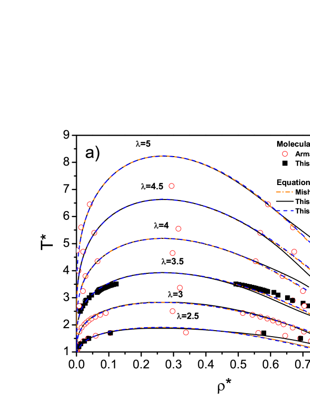
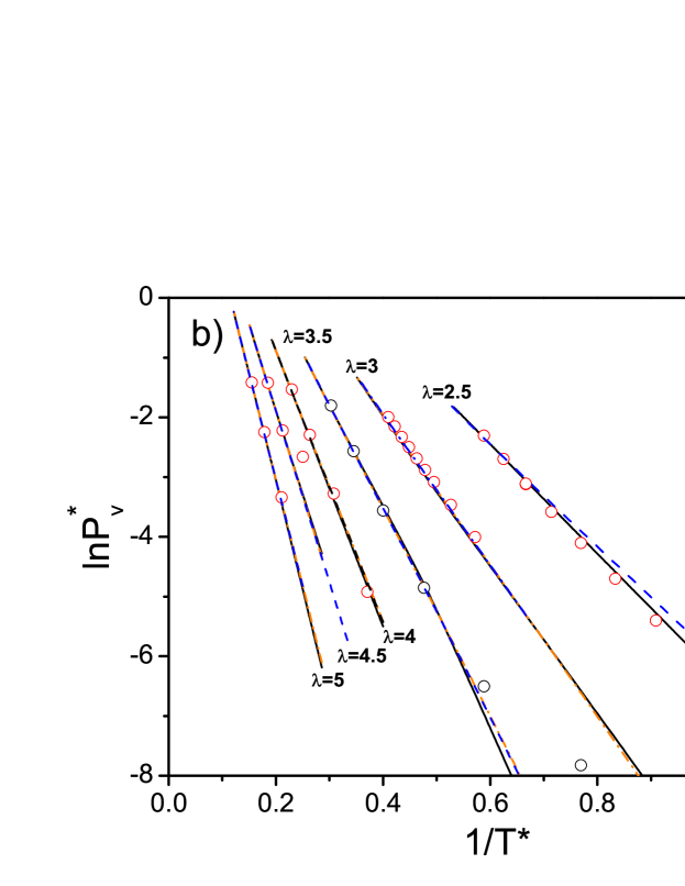
Figure 1: VLE of the SW2D fluid with $\lambda\geq 2.5$. Symbols correspond to the simulation results of Armas et al.Armas-Pérez et al. (2013) (open circles) and our new simulation results (full squares). Dash-dotted lines corresponds to the EoS reported in Ref. Mishra and Sinha, 1984, while the solid and dashed lines are the predictions of the full (solid) and fitted (dashed) EoS described in this work. Here, $T^{*}=kT/|\varepsilon|$, $\rho^{*}=\rho\sigma^{2}$, and $P^{*}=P\sigma^{2}/|\varepsilon|$.

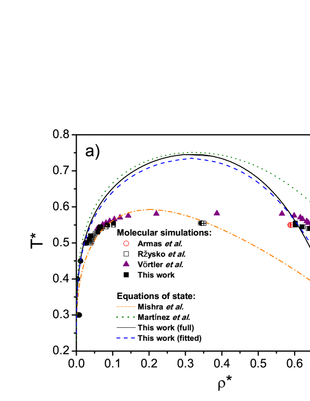
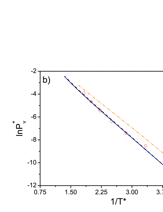
Figure 2: VLE of the SW2D fluid with $\lambda$=1.5. Symbols correspond to the simulation results of Armas et al.Armas-Pérez et al. (2013) (open circles), Rżysko et al.Rżysko et al. (2010) (open squares), Vörtler et al.Vörtler et al. (2008) (full triangles), and our new simulation results (full squares). The dash-dotted and dotted lines corresponds to the EoSs reported in Refs. Mishra and Sinha, 1984; Martínez et al., 2007, respectively, while the solid and dashed lines are the predictions of the full (solid) and fitted (dashed) EoS described in this work.

The vapor-liquid equilibrium (VLE) of SW2D fluids is established here as a severe test of the accuracy of a given EoS. We have separated our results into two figures. In Fig. 1, the VLE is shown for SW2D fluids of long ranges. Our simulation and theoretical results are very close to the simulation results of Armas et al.Armas-Pérez et al. (2013) and to the EoSs of Mishra and SinhaMishra and Sinha (1984) and Martínez et al.Martínez et al. (2007) The approximation of Mishra and Sinha consists in ignoring the fluid structure of the RDF at long distances, i.e., $\delta J(\lambda)\equiv-\sigma^{-2}\int_{\lambda\sigma}^{\infty}dr\,r\left[g^{\text{HD}}(r)-1\right]\approx 0$. This assumption deteriorates the accuracy of the associated EoS for shorter ranges, as can be observed in Fig. 2, which includes additional simulations results of Rżysko et al.Rżysko et al. (2010) and Vörtler et al.Vörtler et al. (2008) The reason behind this behavior can be found in Fig. 6 of the Appendix, where it can be checked that $\delta J$ differs notably from zero at short ranges. It should be noted that the oscillatory behavior of $\delta J$ introduces a nontrivial systematic error that depends strongly on $\lambda$. For $\lambda=1.5$, the EoS of Mishra and Sinha dramatically underestimates the liquid density. In contrast, this liquid branch is overestimated by the SAFT approach.Martínez et al. (2007) The results of the EoS presented in this paper reproduces the VLE with semi-quantitative agreement, while the saturation pressure is accurately described. Remarkably, the apparent density anomaly observed in simulations at low temperatures is also predicted within our approach qualitatively. Similar results have been obtained with the parameterized EoS described in Sec. II.2. It should be pointed out that the accuracy of PTs worsens as the dimensionality decreases. Moreover, in 2D fluids, the VLE exhibits a high flatness near the critical point that cannot be reproduced by a PT. In all cases, the results obtained with the parameterization described by Eqs. (16)–(II.2) are similar to those obtained with the full calculations employing Eqs. (10).

III.2 Vapor-liquid equilibrium and equation of state of two-dimensional Lennard-Jones fluids

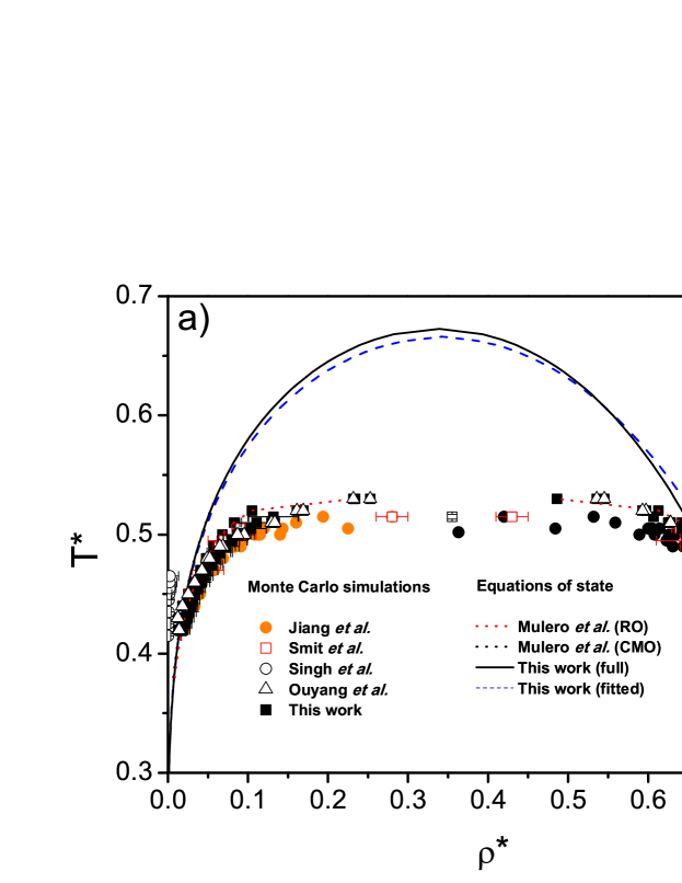
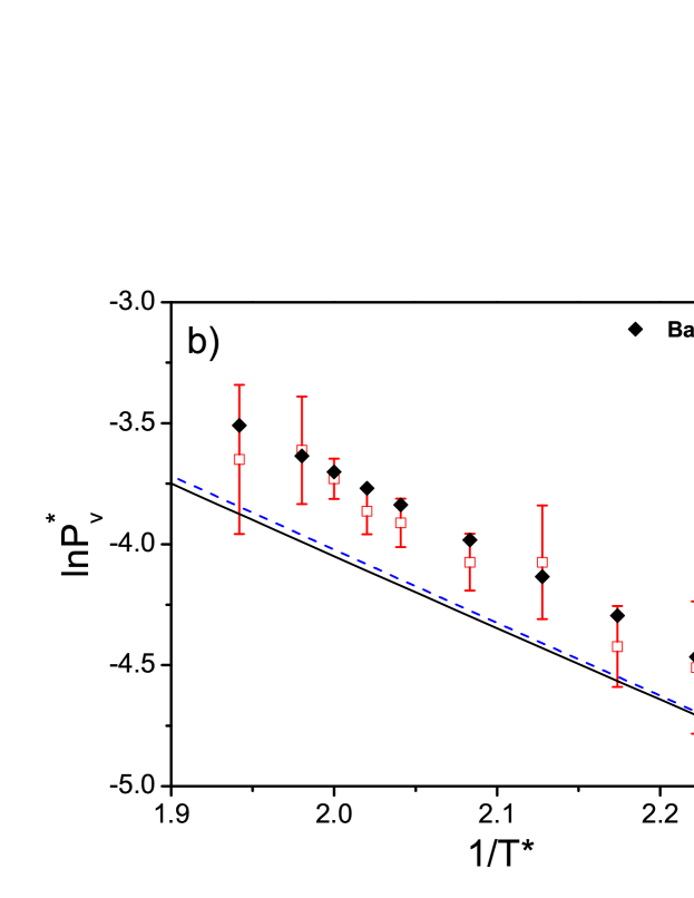
Figure 3: VLE of the LJ2D fluid. Symbols correspond to the simulation results from Refs. Jiang and Gubbins, 1995; Smit and Frenkel, 1991; Singh et al., 1990; Ouyang et al., 2011, the parameterization of Ref. Barker et al., 1981, and the new GEMC results obtained in this work, as labeled in the graph. The solid and dashed lines are the predictions of the full (solid) and fitted (dashed) EoSs described in this work and the semiempirical expresions (denoted as CMO and RO for the Cuadros–Mulero and Reddy–O’Shea EoSs, respectively) of Ref. Mulero et al., 1999

.

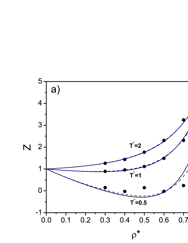
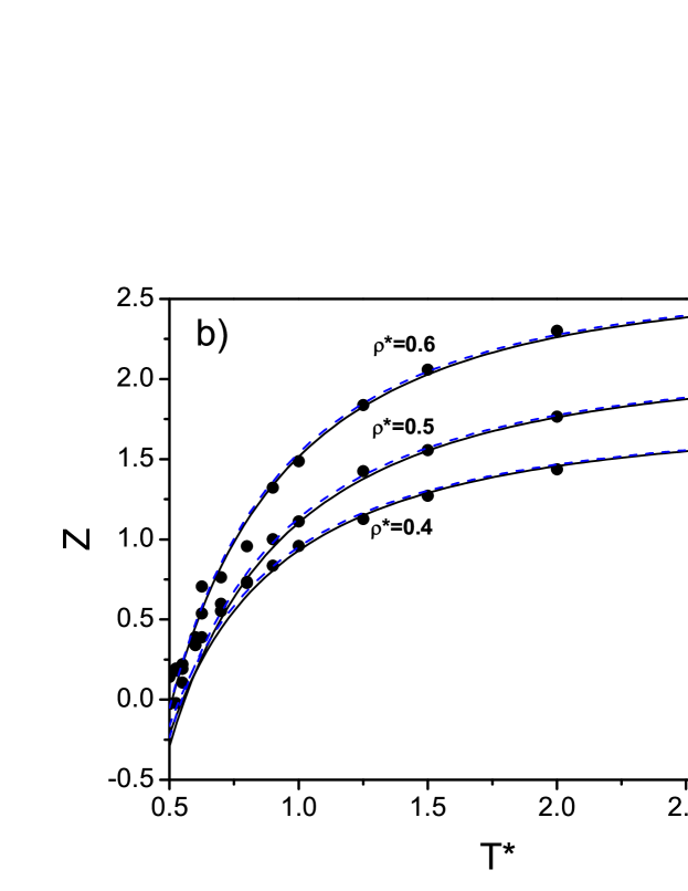
Figure 4: EoS of the LJ2D fluid. Symbols correspond to the simulation results from Ref. Henderson, 1977. The solid and dashed lines are the predictions of the full (solid) and fitted (dashed) EoSs described in this work.

The well-known LJ pair potential is

$$u^{\text{LJ}}(r)=4\varepsilon\left[\left(\frac{\sigma}{r}\right)^{12}-\left(\frac{\sigma}{r}\right)^{12}\right],$$ (25)

where $\sigma$ and $\varepsilon$ are the diameter and the well depth, respectively. The LJ potential is a coarse-grained model extensively used in computer simulations. As such, it has a much higher computational simplicity in comparison with those potentials coming from quantum chemistry calculations, but by the price of being less accurate. In essence, the LJ potential provides a simple description of the repulsive electronic interaction due to the quantum Pauli principle, as well as of the attractive part coming from the induction and dispersive interactions.Lennard-Jones (1924)

The discrete version of the LJ potential is given by Eqs. (19) and (20) with $\lambda_{p}=\lambda_{c}$, where $\lambda_{c}$ is a cutoff distance for the LJ tail. It can be calculated by requiring $|u^{\text{LJ}}(r)/\varepsilon|<10^{-6}$ for $r>\lambda_{c}\sigma$, which gives $\lambda_{c}\simeq 12.6$. The number of steps is chosen as $p=3$ in the repulsive part of the potential profile ($1\leq r/\sigma\leq 2^{1/6}$) and $p=\lfloor 10({\lambda_{c}-1})\rfloor$, where $\lfloor x\rfloor$ denotes the floor function of argument $x$, in the attractive region ($r/\sigma>2^{1/6}$).

Up to here, a soft potential has been converted into a hard potential. This approximation is reasonably good for some cases treated up to now. However, the integration of the Mayer function would help in the treatment of the repulsive part by mapping the LJ potential onto an effective HD of diameter given in the BH approach as

$$d(\beta)=\int_{0}^{\sigma}dr\,\left\{1-\exp\left[-\beta u^{\text{LJ}}(r)\right]\right\}.$$ (26)

In this work, we have used the parameterization of $d(\beta)$ reported in Ref. Cotterman et al., 1986. This approach is shown to have a positive effect in reproducing the VLE and EoS coming from simulation data of the LJ2D potential.

The resulting VLE coming from both PTs is plotted in Fig. 3 in comparison with our own simulation results and those obtained from different sources in the literature.Jiang and Gubbins (1995); Smit and Frenkel (1991); Singh et al. (1990); Barker et al. (1981); Ouyang et al. (2011) A more pronounced deviation for the saturation pressure, as compared with the SW case, is observed. In fact, the underestimation of the vapor pressure when the perturbation series is truncated to second order is well established in the literature.Fischer et al. (1984). Besides being of semiempirical character, the EoSs in Ref. Mulero et al., 1999 do not substantially improve the agreement of the proposed analytical EoS with the simulation results and, moreover, we avoid the ill-behavior near the critical region observed for those semiempirical formulations.

In Figs. 4 and 4, the compressibility factor $Z$ obtained by MC simulation in Ref. Henderson, 1977 as a function of $\rho^{*}$ and $T^{*}$ in the medium-temperature and density regimes, respectively, is shown. The temperature and density regimes comprise both supercritical and subcritical regions. The agreement of simulation results and our PTs is excellent, except for low temperature and high density, and are of similar accuracy as the semiempirical PT proposed by Henderson.Henderson (1977) The accuracy of the parameterized (fitted) EoS for the SW model is well transferred to the DPT approach, as readily observed in Figs. 3 and 4.

III.3 Vapor-liquid equilibrium of two-dimensional Yukawa fluids

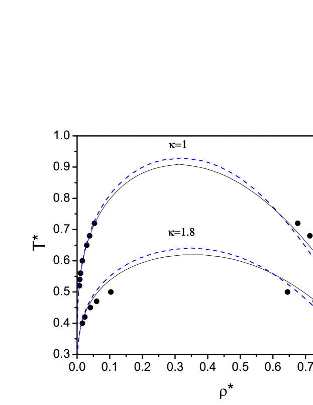
Figure 5: VLE of the 2D Yukawa fluids with $\kappa=1$ and $1.8$. Symbols correspond to simulation results from Ref. M.-Maldonado et al., 2012. The solid and dashed lines are the predictions of the full (solid) and fitted (dashed) EoSs described in this work.

The Yukawa (or screening Coulomb) potential has become popular nowadays in soft matter physics in the description of the electrostatic interaction between colloids and other mesoscopic systems in the dilute limit.Hiemenz and Rajagopalan (1997) Its functional form is given by

$$u^{\text{Y}}(r)=\begin{cases}\infty,&r<\sigma,\\ \displaystyle{-\varepsilon\frac{\exp[-\kappa(r/\sigma-1)]}{r/\sigma}},&r>\sigma,\end{cases}$$ (27)

where $\kappa$ is the (reduced) inverse screening length. Its discrete version can again be constructed from Eqs. (19) and (20), with $p=\lfloor 10({\lambda_{c}-1})\rfloor$ and a cutoff value $\lambda_{p}=\lambda_{c}$ such that $|u^{\text{Y}}(\lambda_{c}\sigma)/\varepsilon|=10^{-6}$. The solution is $\lambda_{c}=W(10^{6}\kappa e^{\kappa})/\kappa$, where $W(x)$ is the Lambert function.

To the best of our knowledge, the only available results for the 2D Yukawa model can be found in Ref. M.-Maldonado et al., 2012, but with a slightly different functional form, as required for the molecular dynamics method employed there. Given the peculiar results obtained in Ref. M.-Maldonado et al., 2012 for values of $\kappa$ higher than $1.8$ (with densities well above $\rho^{*}=1$), we report our results only for $\kappa=1$ and $1.8$ in Fig. 5. As expected, there is a detrimental effect in the agreement as $\kappa$ increases because it causes the potential to be stiffer. This fact implies a non-optimized sequence of step functions in which some of them present high values of $|\varepsilon_{i}|$, where the high-temperature perturbation expansion no longer holds. This effect has been checked to be crucial for large $\kappa$-values, but it propagates for low $\kappa$-values up to the exact Kac limit $\kappa\rightarrow 0$. As expected, similar conclusions can be traced when using the parameterized EoS.

IV Conclusions

In this paper an EoS for SW2D fluids was obtained in the framework of the high-temperature BH PT.Barker and Henderson (1967a); Barker and Henderson (1967b) The key ingredient in the EoS is an approximate analytical expression for the RDF of HDs proposed in Refs. Yuste and Santos, 1993; Santos and López de Haro, 2016. This equation has been tested against simulation results and other theoretical EoSs. The EoS proposed here shows a better agreement in describing the VLE of a SW2D fluid of middle-short range ($\lambda=1.5$) that those reported in the literature. Besides, this EoS was implemented in an extension of the DPT, originally developed for 3D potentials. Since the HD RDF is not restricted to any value of $\lambda$, the discretization of the potential has a priori no constraints on the potential range, but on the molecular packing.

We have tested the 2D DPT against simulation results for the LJ and Yukawa fluids. Given the perturbative treatment of the attractive part of the interactions, as well as the approximate character of the RDF, our results are in semiquantitative agreement with the reported MC calculations. It seems fair to mention that this EoS constitutes a new member to be included in the scarce list of (analytical) EoSs for 2D fluids. A common feature for PTs is that they do not predict correctly the critical properties because critical fluctuations are neglected. This fact is highlighted in the 2D cases. Some improvement could be achieved by incorporating those fluctuations by the renormalization group theory, as proposed by WhiteA.White (1992); Salvino and White (1992) and successfully applied by Lovell et al.Llovell et al. (2004); Llovell and Vega (2006) to the soft-SAFT EoS.

Finally, the EoS proposed here could be easily extended to incorporate molecular fluids following the assumption given in Refs. Gámez and Benavides (2013); Gámez (2014). This extension of the theory would allow one to reproduce the thermodynamics of molecular systems (as 2D oligomersPatra et al. (2012)), would also serve as a guide for performing computer simulations of layered anisotropic fluids, or could be used as reference in the theoretical modeling of confined liquid crystal phases. Last but not least, given that the RDF employed here owns a general analytical solution for an arbitrary dimension $d$, our results can also be extended to fractal fluids.Torquato (2002)

V Supplementary Material

See the supplementary material for a Fortran 90 code for the evaluation of the integral (41).

*

Appendix A Analytical evaluation of the integral $J(\eta,\lambda)$

In this appendix, the analytical evaluation of the integral $J(\eta,\lambda)$ defined by Eq. (11) is detailed. It is based on the approximate RDF for HDs proposed in Refs. Yuste and Santos, 1993; Santos and López de Haro, 2016.

A.1 Radial distribution function of hard disks

The RDF of HDs is obtained under the assumption that the structure and spatial correlations of HD fluids share some features with those of a hard-rod ($d=1$) and hard-sphere ($d=3$) fluids.Yuste and Santos (1993) The RDF of HDs is given within this approximation as follows,Yuste and Santos (1993); Santos and López de Haro (2016)

$$g(r,\eta)=\alpha(\eta)g^{(1)}\left(r,\gamma_{1}(\eta)\eta\right)+[1-\alpha(\eta)]g^{(3)}\left(r,\gamma_{3}(\eta)\eta\right),$$ (28)

where $g^{(1)}$ is the exact RDF for hard rods,Santos (2016) $g^{(3)}$ is the RDF for hard spheres as obtained from the Percus–Yevick (PY) equation,Wertheim (1963, 1964) and we have simplified the notation $g^{\text{HD}}\to g$. Moreover, the mixing parameter $\alpha$ and the scaling factors $\gamma_{1}$, $\gamma_{3}$ are the following functions of $\eta$:

$$\alpha(\eta)=\frac{H(\eta)-H^{(3)}\left(\gamma_{3}(\eta)\eta\right)}{H^{(1)}\left(\gamma_{1}(\eta)\eta\right)-H^{(3)}\left(\gamma_{3}(\eta)\eta\right)},$$ (29a)

$$\gamma_{1}(\eta)=\frac{g_{\text{cont}}(\eta)-1}{\eta g_{\text{cont}}(\eta)},$$ (29b)

$$\gamma_{3}(\eta)=\frac{1+4g_{\text{cont}}(\eta)-\sqrt{1+24g_{\text{cont}}(\eta)}}{4\eta g_{\text{cont}}(\eta)}.$$ (29c)

Here, the contact values of the RDF for $d=1,2,3$ are given by

$$g^{(1)}_{{\text{cont}}}(\eta)=\frac{1}{1-\eta},$$ (30a)

$$g_{\text{cont}}(\eta)=\frac{1-c\eta}{(1-\eta)^{2}},$$ (30b)

$$g^{(3)}_{{\text{cont}}}(\eta)=\frac{1+\eta/2}{(1-\eta)^{2}}.$$ (30c)

According to the Henderson EoS,Henderson (1975) $c=\frac{7}{16}=0.4375$ in Eq. (30b), but a better value is $c=2\sqrt{3}/\pi-2/3\simeq 0.4360$. In Eq. (29a), the moment

$$H(\eta)=-\int_{0}^{\infty}\text{d}r\,r[g(r,\eta)-1]$$ (31)

for $d=1,2,3$ is

$$H^{(1)}(\eta)=\frac{1}{2}-\frac{2}{3}\eta+\frac{1}{4}\eta^{2},$$ (32a)

$$H(\eta)=\frac{\frac{1}{2}-\frac{1}{4}c\eta(3-\eta)}{1+\eta+(1-2c)\eta^{2}(3-\eta)},$$ (32b)

$$H^{(3)}(\eta)=\frac{\frac{1}{2}-\frac{1}{20}\eta(2-\eta)}{1+2\eta}.$$ (32c)

A.2 Radial distribution function of hard rods

In the case $d=1$, the exact analytical expression for the Laplace transform

$$G^{(1)}(s,\eta)=\int_{0}^{\infty}dr\,e^{-rs}g^{(1)}(r,\eta)$$ (33)

is given byHeying and Corti (2004); Santos (2016)

$$G^{(1)}(s,\eta)=\frac{1}{\eta}\frac{e^{-s}}{1+s(1-\eta)/\eta-e^{-s}},$$ (34)

where, without loss of generality, $\sigma=1$ has been taken as length unit. By expanding $G^{(1)}(s,\eta)$ in powers of $e^{-s}$, the inverse Laplace transform can readily be obtained term by term. Then, the RDF for hard rods $g^{(1)}(r,\eta)$ is given by

$$g^{(1)}(r,\eta)= \frac{1}{\eta}\sum_{\ell=1}^{\infty}\left(\frac{\eta}{1-\eta}\right)^{\ell}\frac{(r-\ell)^{\ell-1}}{(\ell-1)!}$$

$$\times e^{-(r-\ell)\eta/(1-\eta)}\Theta(r-\ell),$$ (35)

where $\Theta(x)$ is the Heaviside step function of argument $x$.

A.3 Radial distribution function of hard spheres

The analytical solution of the PY integral equation in the three-dimensional case ($d=3$) relies upon the Laplace transform of $rg^{(3)}(r,\eta)$,

$$G^{(3)}(s,\eta)=\int_{0}^{\infty}dr\,e^{-rs}rg^{(3)}(r,\eta).$$ (36)

The solution isWertheim (1963, 1964); Hansen and McDonald (2006); Santos (2016)

$$G^{(3)}(s,\eta)=s\frac{F(s,\eta)e^{-s}}{1+12\eta F(s,\eta)e^{-s}},$$ (37)

where

$$F(s,\eta)=-\frac{1}{12\eta}\frac{1+L_{1}(\eta)s}{1+S_{1}(\eta)s+S_{2}(\eta)s^{2}+S_{3}(\eta)s^{3}},$$ (38a)

$$L_{1}(\eta)= \frac{1+\eta/2}{1+2\eta},\quad S_{1}(\eta)=-\frac{3}{2}\frac{\eta}{1+2\eta},$$ (38b)

$$S_{2}(\eta)= -\frac{1}{2}\frac{1-\eta}{1+2\eta},\quad S_{3}(\eta)=-\frac{1}{12\eta}\frac{(1-\eta)^{2}}{1+2\eta}.$$ (38c)

As in the one-dimensional case, the function $G^{(3)}(s,\eta)$ can be expanded in powers of $e^{-s}$, thus allowing to write analytically the RDF as

$$g^{(3)}(r,\eta)=\frac{1}{r}\sum_{\ell=1}^{\infty}\left(-12\eta\right)^{\ell-1}{\Psi}_{\ell}(r-\ell,\eta){\Theta(r-\ell)},$$ (39)

with

$${\Psi}_{\ell}(r,\eta)=\sum_{j=1}^{\ell}\frac{\sum_{i=1}^{3}a_{\ell j}^{(i)}(\eta)e^{s_{i}(\eta)r}}{(\ell-j)!(j-1)!}r^{\ell-j},$$ (40a)

$$a_{\ell j}^{(i)}(\eta)=\lim_{s\to s_{i}}\left(\frac{\partial}{\partial s}\right)^{j-1}\left\{s\left[(s-s_{i})F(s,\eta)\right]^{\ell}\right\},$$ (40b)

where $s_{i}(\eta)$, ($i=1,2,3$) are the three roots of the cubic equation $1+S_{1}(\eta)s+S_{2}(\eta)s^{2}+S_{3}(\eta)s^{3}=0$.

A.4 Analytical evaluation of $J(\eta,\lambda)$

Figure 6: Plot of $\delta J(\eta,\lambda)=J(\eta,\lambda)-\left[\frac{1}{2}\lambda^{2}-H(\eta)\right]$ (a) as a function of $\lambda$ at $\eta=0.5$ and (b) as a function of $\eta$ at $\lambda=1.5$.

Insertion of Eq. (28) into Eq. (11) yields

$$J(\eta,\lambda)=\alpha(\eta)J^{(1)}\left(\gamma_{1}(\eta)\eta,\lambda\right)+[1-\alpha(\eta)]J^{(3)}\left(\gamma_{3}(\eta)\eta,\lambda\right),$$ (41)

where

$$J^{(d)}\left(\eta,\lambda\right)=\int_{1}^{\lambda}dr\,rg^{(d)}(r,\eta).$$ (42)

Thus, we can focus on $J^{(1)}(\eta,\lambda)$ and $J^{(3)}(\eta,\lambda)$.

From Eq. (A.2), $J^{(1)}$ can be rewritten as

$$J^{(1)}= \frac{1}{\eta}\sum_{\ell=1}^{\lfloor\lambda\rfloor}\left(\frac{\eta}{1-\eta}\right)^{\ell}\int_{0}^{\lambda-\ell}dx\,(x+\ell)\frac{x^{\ell-1}}{(\ell-1)!}e^{-x\eta/(1-\eta)}$$

$$= \frac{1}{\eta}\sum_{\ell=1}^{\lfloor\lambda\rfloor}\ell\left[\frac{1-\eta}{\eta}\Phi_{\ell}\left(\frac{\eta(\lambda-\ell)}{1-\eta}\right)+\Phi_{\ell-1}\left(\frac{\eta(\lambda-\ell)}{1-\eta}\right)\right],$$ (43)

where we have introduced the function

$$\Phi_{\ell}(t)\equiv\frac{1}{\ell!}\int_{0}^{t}dx\,e^{-x}x^{\ell}=1-e^{-t}\sum_{j=0}^{\ell}\frac{t^{j}}{j!}.$$ (44)

Next, from Eqs. (39) and (40a), $J^{(3)}$ is given by

$$J^{(3)}= \sum_{\ell=1}^{\lfloor\lambda\rfloor}(-12\eta)^{\ell-1}\int_{0}^{\lambda-\ell}dx\,\Psi_{\ell}(x,\eta)$$

$$= \sum_{\ell=1}^{\lfloor\lambda\rfloor}(-12\eta)^{\ell-1}\sum_{j=1}^{\ell}\frac{1}{(j-1)!}\sum_{i=1}^{3}\frac{a_{\ell j}^{(i)}}{\left(-s_{i}\right)^{\ell-j+1}}$$

$$\times\Phi_{\ell-j}\left(-s_{i}(\lambda-\ell)\right).$$ (45)

By inserting Eqs. (A.4) and (45) into Eq. (41) we find an analytical representation of the integral $J(\eta,\lambda)$. Given a value of $\lambda$, the number of terms in the sums of Eqs. (A.4) and (45) are $\lfloor\lambda\rfloor$, and $3\lfloor\lambda\rfloor(\lfloor\lambda\rfloor+1)/2$, respectively. Thus, from a practical point of view, the above representation might present problems if $\lambda>10$. In that case, it might be convenient to use the asymptotic behavior of $J$ for large $\lambda$. To that end, note the identity [see Eqs. (11) and (31)]

$$J(\eta,\lambda)=\frac{1}{2}\lambda^{2}-H(\eta)+\delta J(\eta,\lambda),$$ (46)

where

$$\delta J(\eta,\lambda)\equiv-\int_{\lambda}^{\infty}dr\,r[g(r,\eta)-1].$$ (47)

If $\lambda$ is large, $\delta J$ can be neglected, so that

$$J(\eta,\lambda)\approx\frac{1}{2}\lambda^{2}-H(\eta).$$ (48)

The dependence of $\delta J(\eta,\lambda)=J(\eta,\lambda)-\left[\frac{1}{2}\lambda^{2}-H(\eta)\right]$ as a function of both $\lambda$ and $\eta$ is shown in Fig. 6. As seen in Fig. 6, Eq. (48) is an excellent approximation for $\lambda>10$. On the other hand, as expected, $\delta J$ is non-negligible if $\lambda$ is not very far from $1$. Figure 6 shows that $\delta J$ presents an oscillatory behavior with respect to density.

The Fortran 90 program for evaluating the function $J(\eta,\lambda)$ is included as supplementary material.

References

- Hansen and McDonald (2006) J.-P. Hansen and I. R. McDonald, Theory of Simple Liquids (Academic, London, 2006).
- Solana (2013) J. R. Solana, Perturbation Theories for the Thermodynamic Properties of Fluids and Solids (CRC Press, Boca Raton, 2013).
- Santos (2016) A. Santos, A Concise Course on the Theory of Classical Liquids. Basics and Selected Topics, vol. 923 of Lecture Notes in Physics (Springer, New York, 2016).
- Rowlinson (1979) J. S. Rowlinson, J. Stat. Phys. 20, 197 (1979).
- Barker and Henderson (1967a) J. A. Barker and D. Henderson, J. Chem. Phys. 47, 2856 (1967a).
- Barker and Henderson (1967b) J. A. Barker and D. Henderson, J. Chem. Phys. 47, 4714 (1967b).
- Chandler and Weeks (1970) D. Chandler and J. D. Weeks, Phys. Rev. Lett. 25, 149 (1970).
- Henderson and Barker (1970) D. Henderson and J. A. Barker, Phys. Rev. A 1, 1266 (1970).
- Weeks et al. (1971) J. D. Weeks, D. Chandler, and H. C. Andersen, J. Chem. Phys. 54, 5237 (1971).
- Zhou and Solana (2009) S. Zhou and J. R. Solana, Chem. Rev. 109, 2829 (2009).
- Phillips et al. (1981) J. M. Phillips, L. W. Bruch, and R. D. Murphy, J. Chem. Phys. 75, 5097 (1981).
- Reddy and O’Shea (1986) M. R. Reddy and S. F. O’Shea, Can. J. Phys. 64, 677 (1986).
- Rovere et al. (1990) M. Rovere, D. W. Heermanns, and K. Binder, J. Phys. Condens. Matter 2, 7009 (1990).
- Löwen (1992) H. Löwen, J. Phys. Condens. Matter 4, 10105 (1992).
- Mulero et al. (1999) A. Mulero, F. Cuadros, and C. Faúndez, Aust. J. Phys. 52, 101 (1999).
- Ouyang et al. (2011) W. Z. Ouyang, S. H. Xu, and Z. W. Sun, Chinese Sci. Bull. 56, 2773 (2011).
- Khordad (2012) R. Khordad, Commun. Theor. Phys. 58, 759 (2012).
- Murillo and Gericke (2003) M. S. Murillo and D. O. Gericke, J. Phys. A: Math. Gen. 36, 6273 (2003).
- Lang et al. (2014) S. Lang, T. Franosch, and R. Schilling, J. Chem. Phys. 140, 104506 (2014).
- Vaulina and Koss (2014) O. Vaulina and X. Koss, Physics Letters A 378, 3475 (2014).
- Kryuchkov et al. (2017) N. P. Kryuchkov, S. A. Khrapak, and S. O. Yurchenko, J. Chem. Phys. 146, 134702 (2017).
- Mishra and Sinha (1984) B. M. Mishra and S. K. Sinha, Pramana 23, 79 (1984).
- Henderson (1977) D. Henderson, Mol. Phys. 34, 301 (1977).
- Buenrostro-González et al. (2004) E. Buenrostro-González, C. Lira-Galeana, A. Gil-Villegas, and J. Wu, AIChE J. 50, 2552 (2004).
- Martínez et al. (2007) A. Martínez, M. Castro, C. McCabe, and A. Gil-Villegas, J. Chem. Phys. 126, 074707 (2007).
- Jiménez-Serratos et al. (2008) G. Jiménez-Serratos, S. Santillán, C. Avendaño, M. Castro, and A. Gil-Villegas, Oil & Gas Sci. Tech. 63, 329 (2008).
- Castro et al. (2009) M. Castro, J. L. M. de la Cruz, E. Buenrostro-González, S. López-Ramírez, and A. Gil-Villegas, Fluid Phase Equilibria 87, 113 (2009).
- Trejos et al. (2014) V. M. Trejos, M. Becerra, S. F.-Gerstenmaier, and A. Gil-Villegas, Mol. Phys. 112, 2330 (2014).
- Martínez et al. (2017) A. Martínez, V. M. Trejos, and A. Gil-Villegas, Fluid Phase Equilibria 449, 207 (2017).
- Castro et al. (2011) M. Castro, A. Martínez, and A. Gil-Villegas, Adsorption Sci. Technol. 29, 59 (2011).
- Castro and Martínez (2013) M. Castro and A. Martínez, Adsorption 63, 63 (2013).
- Trejos et al. (2018) V. M. Trejos, A. Martínez, and A. Gil-Villegas, Fluid Phase Equilibria 462, 153 (2018).
- Benavides and Gil-Villegas (1999) A. L. Benavides and A. Gil-Villegas, Mol. Phys. 97, 1225 (1999).
- Chapela et al. (2010) G. A. Chapela, F. del Rio, A. L. Benavides, and J. Alejandre, J. Chem. Phys. 133, 234107 (2010).
- Benavides and Gámez (2011) A. L. Benavides and F. Gámez, J. Chem. Phys. 135, 134511 (2011).
- Gámez and Benavides (2013) F. Gámez and A. L. Benavides, J. Chem. Phys. 138, 124901 (2013).
- Gámez (2014) F. Gámez, J. Chem. Phys. 140, 234504 (2014).
- Cervantes et al. (2015) L. A. Cervantes, G. Jaime-Muñoz, A. L. Benavides, J. Torres-Arenas, and F. Sastre, J. Chem. Phys. 142, 114501(1) (2015).
- Yuste and Santos (1993) S. B. Yuste and A. Santos, J. Chem. Phys. 99, 2020 (1993).
- Santos and López de Haro (2016) A. Santos and M. López de Haro, Phys. Rev. E 93, 062126 (2016).
- Henderson (1975) D. Henderson, Mol. Phys. 30, 971 (1975).
- Gil-Villegas et al. (1997) A. Gil-Villegas, A. Galindo, P. J. Whitehead, S. J. Mills, G. Jackson, and A. N. Burgess, J. Chem. Phys. 106, 4168 (1997).
- Patel et al. (2005) B. H. Patel, H. Docherty, A. G. S. Varga, and G. C. Maitland, Mol. Phys. 103, 129 (2005).
- Panagiotopoulos (1987) A. Z. Panagiotopoulos, Mol. Phys. 61, 813 (1987).
- Armas-Pérez et al. (2013) J. C. Armas-Pérez, J. Quintana-H, and G. A. Chapela, J. Chem. Phys. 138, 044508 (2013).
- Rżysko et al. (2010) W. Rżysko, A. Patrykiejew, S. Sokołowski, and O. Pizio, J. Chem. Phys. 132, 164702 (2010).
- Vörtler et al. (2008) H. L. Vörtler, K. Schöafer, and W. R. Smith, J. Chem. Phys. 112, 4656 (2008).
- Jiang and Gubbins (1995) S. Jiang and K. E. Gubbins, Mol. Phys. 86, 599 (1995).
- Smit and Frenkel (1991) B. Smit and D. Frenkel, J. Chem. Phys. 94, 5663 (1991).
- Singh et al. (1990) R. Singh, K. Pitzer, J. de Pablo, and J. Prausnitz, J. Chem. Phys. 92, 5463 (1990).
- Barker et al. (1981) J. A. Barker, D. Henderson, and F. F. Abraham, Physica A 106, 226 (1981).
- Lennard-Jones (1924) J. Lennard-Jones, Proc. R. Soc. Lond., Ser. A 106, 441 (1924).
- Cotterman et al. (1986) R. L. Cotterman, B. J. Schwarz, and J. M. Prausnitz, AIChE J. 32, 1787 (1986).
- Fischer et al. (1984) J. Fischer, R. Lustig, H. Breitenfelder-Manske, and W. Lemming, Mol. Phys. 52, 485 (1984).
- M.-Maldonado et al. (2012) G. A. M.-Maldonado, M. G.-Melchor, and J. Alejandre, Condens. Matter Phys. 15, 23002 (2012).
- Hiemenz and Rajagopalan (1997) P. Hiemenz and R. Rajagopalan, Principles of Colloid and Surface Chemistry (Marcel Dekker, New York, 1997), 3rd ed.
- A.White (1992) J. A.White, Fluid Phase Equilibria 75, 53 (1992).
- Salvino and White (1992) L. W. Salvino and J. A. White, J. Chem. Phys. 96, 4559 (1992).
- Llovell et al. (2004) F. Llovell, J. C. Pámies, and L. F. Vega, J. Chem. Phys. 121, 10715 (2004).
- Llovell and Vega (2006) F. Llovell and L. F. Vega, J. Phys. Chem. B 110, 11427 (2006).
- Patra et al. (2012) T. K. Patra, A. Hens, and J. K. Singh, J. Chem. Phys. 137, 084701 (2012).
- Torquato (2002) S. Torquato, Random Heterogeneous Materials: Microstructure and Macroscopic Properties (Springer, New York, NY, 2002).
- Wertheim (1963) M. S. Wertheim, Phys. Rev. Lett. 10, 321 (1963).
- Wertheim (1964) M. S. Wertheim, J. Math. Phys. 5, 643 (1964).
- Heying and Corti (2004) M. Heying and D. S. Corti, Fluid Phase Equilib. 220, 85 (2004).