One-half of the Kibble-Zurek quench followed by free evolution

Abstract

We drive the one-dimensional quantum Ising chain in the transverse field from the paramagnetic phase to the critical point and study its free evolution there. We analyze excitation of such a system at the critical point and dynamics of its transverse magnetization and Loschmidt echo during free evolution. We discuss how the system size and quench-induced scaling relations from the Kibble-Zurek theory of non-equilibrium phase transitions are encoded in quasi-periodic time evolution of the transverse magnetization and Loschmidt echo.

I Introduction

Suppose we prepare a system, which possesses a quantum phase transition, in the ground state of a gapped phase far away from the critical point. Then, we drive it through a gradual change of some parameter of its Hamiltonian to the critical point, where changes of the Hamiltonian stop and the system is let to undergo free evolution. The question we would like to address here is how such free evolution reflects the universal non-equilibrium excitation of the system and the fact that it takes place at the critical point.

The above quench protocol can be seen as combination of continuous and sudden quench protocols that have been intensively studied lately. In the former, the system is driven through a smooth change of some parameter across the critical point. Its non-equilibrium final state is then typically analyzed far away from the critical point in the new phase Jac (a); Dut . In the latter, the instantaneous change of some parameter is imposed on the system and subsequent non-equilibrium free evolution is analyzed Jac (a); Pol (a). In our case, we focus on free evolution, just as in the sudden quench, but take as the initial state the non-equilibrium state of the system resulting from continuous driving to the critical point. That such a quench protocol can lead to interesting results can be seen in the following way.

Prepare finite but large-enough system (6) in the ground state, assume that its evolution towards the critical point is initially adiabatic, and choose linear in time change of the external field driving the transition

$$g(t)=g_{c}-\frac{t}{\tau_{Q}},$$ (1)

where $g_{c}$ is the critical point and $\tau_{Q}$ is the quench time inversely proportional to the driving rate. Evolution of the system cannot be adiabatic all the way to the critical point because the gap in the excitation spectrum becomes too small near the critical point. The crossover from adiabatic to non-adiabatic dynamics is then studied through the quantum version BDP (a); Dor ; Jac (b) of the Kibble-Zurek theory of non-equilibrium phase transitions Kib ; Zur ; del (a, b).

One notices in this approach that there are two time scales determining system’s dynamics. The first one is proportional to the inverse of the instantaneous energy gap $\Delta$ between the ground state and the first excited state. It can be seen as the reaction time of the system: the larger the gap is, the quicker the system adjusts to driving. The second time scale quantifies how fast the system is driven and so it is inversely proportional to rate at which the gap changes, $\Delta/\frac{d}{dt}\Delta$. The crossover between the adiabatic regime and the non-equilibrium one takes place when these two time scales become comparable

$$\frac{\hbar}{\Delta}\sim\frac{\Delta}{\frac{d}{dt}\Delta}.$$ (2)

Such an equation can be solved by combining (1) with the standard scaling relation $\Delta\sim|g_{c}-g|^{z\nu}$, where $z$ and $\nu$ are the dynamical and correlation-length exponents, respectively. The solution gives scaling of the distance $\hat{g}$ from the critical point, where the crossover takes place

$$\hat{g}\sim\tau_{Q}^{-1/(1+z\nu)}.$$ (3)

Using this result, one can also obtain scaling of the time that is left to reaching the critical point from the moment when the system enters the crossover regime

$$\hat{t}=\hat{g}\tau_{Q}\sim\tau_{Q}^{z\nu/(1+z\nu)}.$$ (4)

Besides the characteristic field and time scales, $\hat{g}$ and $\hat{t}$, respectively, the Kibble-Zurek theory implies existence of the characteristic quench-induced length scale

$$\hat{\xi}=\xi(\hat{g})\sim\tau_{Q}^{\nu/(1+z\nu)},$$ (5)

where $\xi$ is the equilibrium correlation length. Finite-size effects in the Kibble-Zurek quench (1) are negligible when the system size $N$ satisfies

$$N\gg\hat{\xi}.$$ (6)

Different observables, computed in the non-equilibrium state of the system after the Kibble-Zurek quench, should scale non-trivially with the quench rate akin to (3)–(5). It is now interesting to ask how they would behave in the time domain during free evolution at the critical point?

The only quench-independent characteristic time scale that we have at the critical point, which is relevant for slowly driven systems being of interest here, is the inverse of the typical energy gap between low-lying energy levels. Taking the standard dispersion relation at the critical point,

$$\omega(k)\sim k^{z},$$ (7)

and noting that $k\sim 1/N$, one finds the characteristic time scale

$$\tau_{c}\sim N^{z},$$ (8)

which is divergent in the thermodynamic limit. Before moving on, we note that (6) is equivalent to the condition that the gap between the ground state and the first excited state at the distance $\hat{g}$ from the critical point, which is proportional to $\hat{g}^{z\nu}\sim 1/\hat{t}$, is much larger than the gap at the critical point that is proportional to $1/\tau_{c}$. This leads to

$$\tau_{c}\gg\hat{t},$$ (9)

which is the same as (6).

The goal of this work is to discuss how Kibble-Zurek scaling relations (3)–(5) and system-size dependent time scale (8) are encoded in free evolution of the one-dimensional quantum Ising model in the transverse field that was driven to the critical point. This system is a standard testbed for various studies of non-equilibrium dynamics. Different aspects of its continuous quenches were researched in numerous references, see e.g. Jac (b); Dor ; Pol (b); Ral ; Pol (c); Sen (a); San (a); Jac (c); Sen (b); Arn (a); Kol ; Fra ; San (b); Pus ; Apo . Significant efforts were also devoted to investigations of sudden quenches in this model, see e.g. Sen (c); Cal (a, b); Arn (b); Ved ; Ess ; Hey (a); Arn (c).

Free dynamics of a quantum system driven to the critical point was theoretically studied in BDN , where the system of interest was a weakly-correlated spin-1 Bose-Einstein condensate. Its dynamics was modeled by the mean-field theory approximating system’s behavior in the thermodynamic limit. It was found that non-trivial oscillations of magnetization take place at the critical point during free evolution following the Kibble-Zurek quench. Their non-triviality followed from the fact that their amplitude was inversely proportional to their period, which was proportional to $\hat{t}$. It is of interest in this work to find out whether comparably-interesting dynamics can be found in a strongly-correlated many-body system such as the quantum Ising chain.

This paper is organized as follows. Basic information about the quantum Ising model is provided in Sec. II. A continuous quench of this system towards the critical point is described in Sec. III. Dynamics of the transverse magnetization and Loschmidt echo during free evolution at the critical point is studied in Secs. IV and V, respectively. Brief summary of our results is available in Sec. VI.

II Model

We study the one-dimensional quantum Ising model in the transverse field described by the following Hamiltonian

$$\hat{H}(g)=-\sum_{i=1}^{N}\!\left(\sigma^{x}_{i}\sigma^{x}_{i+1}+g\sigma^{z}_{i}\right),$$ (10)

where $g$ is the external magnetic field and $N$ is the number of spins. We impose periodic boundary conditions on the system and take even $N$.

This model undergoes a quantum phase transition and it is exactly solvable, which greatly facilitates its study. Its basic equilibrium properties were described in the following seminal references Lie ; Pfe . For the purpose of this work, we need to state that there is the critical point $g_{c}=1$ separating the ferromagnetic phase ($0<g<1$) from the paramagnetic phase ($g>1$). The critical exponents of this model are $z=\nu=1$. This means that

$$\hat{t}\sim\sqrt{\tau_{Q}},\ \tau_{c}\sim N,$$ (11)

$$\hat{\xi}\sim\sqrt{\tau_{Q}}.$$ (12)

We will consider below system sizes

$$N\gg\sqrt{\tau_{Q}}$$ (13)

to satisfy condition (6).

The quench protocol, which we have proposed in Sec. I, reads

$$g(t)=\left\{\begin{array}[]{ll}1-t/\tau_{Q}&\ \text{for}\ t\leq 0\\ 1&\ \text{for}\ t>0\end{array}\right..$$ (14)

Evolution starts from the ground state of Hamiltonian (10) deeply in the paramagnetic phase and the system evolves towards the critical point arriving there in an excited state at $t=0$. The degree of excitation is controlled by the quench time $\tau_{Q}$ (larger $\tau_{Q}$ leads to more adiabatic evolution). Once the critical point is reached, the magnetic field is no longer changed so that the system undergoes free evolution there.

III Dynamics towards the critical point

Time evolution of the quantum Ising model can be most conveniently described by mapping spins onto non-interacting fermions through the Jordan-Wigner transformation Jac (b). Such a transformation reads

$$\sigma^{z}_{i}=1-2\hat{c}_{i}^{\dagger}\hat{c}_{i},\ \ \sigma^{x}_{i}=(\hat{c}_{i}+\hat{c}_{i}^{\dagger})\prod_{j<i}\!\left(1-2\hat{c}_{j}^{\dagger}\hat{c}_{j}\right),$$ (15)

where $\hat{c}_{i}$ are fermionic operators. One then notes that the Hamiltonian commutes with the parity operator

$$\prod_{i=1}^{N}\sigma^{z}_{i},$$ (16)

whose eigenvalues are $\pm 1$. This has two consequences. First, eigenvalues of $\hat{H}$ can be assigned definite parity, positive or negative. Second, if the system is initially prepared in the state with definite parity, then during time evolution only states with such parity are populated. We start evolution from the ground state, which for even-sized systems that we consider, has positive parity BDJ . Therefore, we focus below on the dynamics in the positive-parity subspace of the Hilbert space, where anti-periodic boundary conditions are imposed on fermionic operators: $\hat{c}_{N+1}=-\hat{c}_{1}$ BDJ .

One then goes to the momentum space through the substitution

$$\hat{c}_{j}=\frac{\exp(-\mathrm{i}\pi/4)}{\sqrt{N}}\sum_{K=\pm k}\hat{c}_{K}\exp(\mathrm{i}Kj),$$ (17)

$$k=\frac{\pi}{N},\frac{3\pi}{N},\cdots,\pi-\frac{\pi}{N},$$ (18)

where $\hat{c}_{\pm k}$ annihilates a quasi-particle with quasi-momentum $\pm k$. After these transformations, one obtains

$$\hat{H}=2\sum_{k}(\hat{c}_{k}^{\dagger}\hat{c}_{k}-\hat{c}_{-k}\hat{c}_{-k}^{\dagger})[g-\cos(k)]+(\hat{c}_{k}^{\dagger}\hat{c}_{-k}^{\dagger}+\hat{c}_{-k}\hat{c}_{k})\sin(k),$$ (19)

which can be diagonalized through the Bogolubov transformation. The ground state of this Hamiltonian is

$$|g\rangle=\prod_{k}\!\left(u_{k}^{\text{eq}}-v_{k}^{\text{eq}}\hat{c}_{k}^{\dagger}\hat{c}_{-k}^{\dagger}\right)|{\rm vac}\rangle,$$ (20)

$$u_{k}^{\text{eq}}=\cos\!\left(\frac{\theta_{k}}{2}\right),\ v_{k}^{\text{eq}}=\sin\!\left(\frac{\theta_{k}}{2}\right),$$ (21)

$$\sin\theta_{k}=\frac{\sin(k)}{\sqrt{g^{2}-2g\cos(k)+1}},\ \ \cos\theta_{k}=\frac{g-\cos(k)}{\sqrt{g^{2}-2g\cos(k)+1}},$$ (22)

where $u_{k}^{\text{eq}}$ and $v_{k}^{\text{eq}}$ are the equilibrium Bogolubov modes and $|{\rm vac}\rangle$ is annihilated by all $\hat{c}_{\pm k}$ operators.

Solving the time-dependent Schrödinger equation, $\mathrm{i}\frac{d}{dt}|\psi(t)\rangle=\hat{H}[g(t)]|\psi(t)\rangle$, one finds that dynamics of the $N$ spin system splits into dynamics of $N/2$ uncoupled Landau-Zener systems. The wave-function can be then written as Jac (b)

$$|\psi(t)\rangle=\prod_{k}\!\left(u_{k}(t)-v_{k}(t)\hat{c}_{k}^{\dagger}\hat{c}_{-k}^{\dagger}\right)|{\rm vac}\rangle,$$ (23)

where $u_{k}$ and $v_{k}$ are the time-dependent Bogolubov modes evolving according to

$$\mathrm{i}\frac{d}{dt}\left(\begin{array}[]{c}v_{k}\\ u_{k}\end{array}\right)=h_{k}\left(\begin{array}[]{c}v_{k}\\ u_{k}\end{array}\right),\ h_{k}=2\left(\begin{array}[]{cc}g(t)-\cos(k)&-\sin(k)\\ -\sin(k)&\cos(k)-g(t)\end{array}\right).$$ (24)

Evolution starts at $t=-\infty$ from the state, where all spins are perfectly aligned with the magnetic field. In the non-interacting fermions formalism this translates into the following initial conditions

$$|u_{k}(t=-\infty)|=1,\ v_{k}(t=-\infty)=0.$$ (25)

This means that all two-level systems (24) start evolution from the ground state of the Hamiltonian $h_{k}$ and results in the following exact solution

$$v_{k}(t)=\sqrt{\tau_{Q}}\sin(k)e^{-\pi\tau_{Q}\sin^{2}(k)/4}D_{-n-1}[\mathrm{i}z(t)],$$ (26)

$$u_{k}(t)=e^{-\pi\tau_{Q}\sin^{2}(k)/4}e^{-\mathrm{i}\pi/4}\!\left((1+n)D_{-n-2}[\mathrm{i}z(t)]+\mathrm{i}z(t)D_{-n-1}[\mathrm{i}z(t)]\right),$$ (27)

$$\mathrm{i}z(t)=2\sqrt{\tau_{Q}}e^{\mathrm{i}\pi/4}[g(t)-\cos(k)],\ n=\mathrm{i}\tau_{Q}\sin^{2}(k),$$ (28)

where $D_{m}$ is the Weber function Wat . We obtained such a solution by mapping (24) into the Landau-Zener form Jac (b)

$$\mathrm{i}\frac{d}{dt^{\prime}}\left(\begin{array}[]{c}u_{k}\\ v_{k}\end{array}\right)=\frac{1}{2}\left(\begin{array}[]{lr}t^{\prime}/\tau_{Q}^{\prime}&1\\ 1&-t^{\prime}/\tau_{Q}^{\prime}\end{array}\right)\left(\begin{array}[]{c}u_{k}\\ v_{k}\end{array}\right),$$ (29)

$$t^{\prime}=4\tau_{Q}\sin(k)[g(t)-\cos(k)],\ \tau_{Q}^{\prime}=4\tau_{Q}\sin^{2}(k),$$

and then adopting to the current problem the steps from Appendix B of BDP (b). Eqs. (26) and (27) can be used for deriving analytical approximations. They are, however, impractical for getting exact results, which we obtain by direct numerical integration of (24).

Having these results, we can quantify the level of excitation at the critical point to better characterize the initial state for subsequent free evolution that we describe in Secs. IV and V. We compute the probability of finding the Ising chain in the ground state at $t=0$

$$p_{GS}=\prod_{k}(1-p_{k})=\exp\!\left(\sum_{k}\ln(1-p_{k})\right),$$ (30)

where $p_{k}$ is the probability of finding two-level system (24) in the excited state at $t=0$. We could, of course, write (30) as the product of probabilities of finding two-level systems (24) in the ground state, but such a representation is inconvenient given analytical approximations that we will use–see discussion around (41) and (42).

A simple calculation then shows that

$$p_{k}=\!\left|v_{ck}^{\text{eq}}\,u_{k}(0)-u_{ck}^{\text{eq}}\,v_{k}(0)\right|^{2},$$ (31)

$$v_{ck}^{\text{eq}}=\cos(k/4+\pi/4),$$ (32)

$$u_{ck}^{\text{eq}}=\sin(k/4+\pi/4),$$ (33)

where $v_{ck}^{\text{eq}}$ and $u_{ck}^{\text{eq}}$ are the equilibrium Bogolubov modes (21) computed at the critical point.

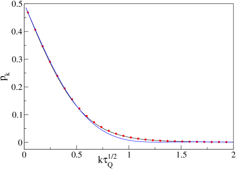
Figure 1: Probability of finding two-level system (24) in the ground state at $t=0$. The black line shows numerics for $\tau_{Q}=100$ (data points are connected by a line). Red dots show numerics for $\tau_{Q}=500$. The blue line shows the approximate result obtained after putting (36)–(38) into (31). The system size $N=2000$.

The basic expectation from the KZ theory is that small $k$ modes are excited during evolution towards the critical point, i.e.,

$$k\lesssim 1/\hat{\xi}\sim 1/\sqrt{\tau_{Q}}.$$ (34)

As a result, we expect that for such momenta $p_{k}$ is a function of $k\sqrt{\tau_{Q}}$. This expectation cannot be exact as the argument of Weber functions at the critical point is

$$iz(0)\sim\sqrt{\tau_{Q}}k^{2}=(k\sqrt{\tau_{Q}})^{2}/\sqrt{\tau_{Q}}$$ (35)

for small momenta. Nonetheless, such dependence is suppressed for large-enough $\tau_{Q}$. Thus, the following approximations, when put into (31), lead to fairly accurate results

$$v_{k}(0)\approx\sqrt{\tau_{Q}}k\sqrt{\frac{\pi}{2}}e^{-\pi\tau_{Q}k^{2}/4},$$ (36)

$$u_{k}(0)\approx e^{-\pi\tau_{Q}k^{2}/4}e^{-\mathrm{i}\pi/4}\!\left[1+\frac{\mathrm{i}}{2}\tau_{Q}k^{2}(\gamma+\ln 2)\right],$$ (37)

$$v_{ck}^{\text{eq}}\approx u_{ck}^{\text{eq}}\approx\frac{1}{\sqrt{2}},$$ (38)

where $\gamma=0.5772\cdots$. The scaling properties of $p_{k}$ are illustrated in Fig. 1. It is worth to note that we expand in a series in $k$ the argument of $e^{-\pi\tau_{Q}\sin^{2}(k)/4}$ instead of the whole exponential function. This amounts to introducing the Gaussian cut-off function,

$$e^{-\pi\tau_{Q}k^{2}/4},$$ (39)

which makes non-equilibrium approximations (36) and (37) vanish for the momenta

$$k\gg 1/\hat{\xi}\sim 1/\sqrt{\tau_{Q}}$$ (40)

for which equilibrium solutions (32) and (33) well approximate exact non-equilibrium solutions (26) and (27), respectively. Such a procedure allows us to separate the non-equilibrium effects from the equilibrium ones, which simplifies the following computations. It was first employed in Jac (b).

We can now explain why it is convenient to use the expression for $p_{GS}$ in the form given by (30). Suppose, we write

$$p_{GS}=\prod_{k}P_{k},$$ (41)

where $P_{k}$ is the probability of finding the two level system (24) in the ground state. A simple calculation then yields

$$P_{k}=\!\left|v_{ck}^{\text{eq}}\,v^{*}_{k}(0)+u_{ck}^{\text{eq}}\,u^{*}_{k}(0)\right|^{2}.$$ (42)

Putting approximations (36) and (37) into (31) and (42), we get for large-momenta, such as (40), that $p_{k},P_{k}\to 0$. In this limit, however, we should be getting $p_{k}\to 0$ and $P_{k}\to 1$ because the modes with large-enough momenta are only marginally excited during our time evolutions. As a result, it is convenient to use expression (30) instead of (41) to compute $p_{GS}$ because in the former case we can use approximate expressions for all momenta without introducing significant errors, while in the latter case restriction to momenta satisfying (34) has to be enforced in the product over $k$.

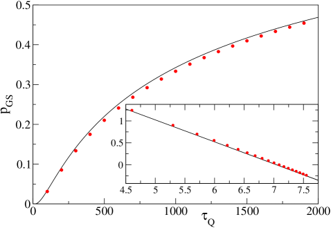
Figure 2: Probability of finding the Ising chain in the ground state at $t=0$. Solid black line shows analytical approximation (45), while red dots provide numerics. The inset shows $\ln[-\ln(p_{GS})]$ vs. $\ln(\tau_{Q})$. The system size $N=1000$.

To further simplify calculations, we approximate for $N\gg 1$ the sum in (30) by the integral

$$\sum_{k}\to\frac{N}{2\pi}\int_{0}^{\pi}dk,$$ (43)

which leads to

$$p_{GS}=\exp\!\left(\frac{N}{2\pi}\int_{0}^{\pi}dk\ln(1-p_{k})\right).$$ (44)

Putting (36)–(38) into (31) and taking $\tau_{Q}\gg 1$, we can rewrite it as

$$p_{GS}\approx\exp\!\left(-C\frac{N}{\sqrt{\tau_{Q}}}\right),$$ (45a)

$$C=-\frac{1}{2\pi}\int_{0}^{\infty}dx\ln\left(1-\frac{1}{8}e^{-\pi x^{2}/2}[(x\sqrt{\pi}-2)^{2}+(x\sqrt{\pi}-x^{2}(\gamma+\ln 2))^{2}]\right)\approx 0.034.$$ (45b)

Comparison between (45) and numerics is presented in Fig. 2, where quite good agreement is found.

Result (45a) can be also obtained through the adiabatic–impulse approximation (AIA) introduced in the quantum context in BDP (a, b). We will adopt this approximation to the problem studied in this paper. In the spirit of AIA, we split evolution towards the critical point into adiabatic and impulse stages. The adiabatic stage takes place when the system is far away from the critical point, which happens when $g(t)-1>\hat{g}$. AIA assumes that populations of instantaneous eigenstates of the Hamiltonian do not change when this condition is satisfied. The impulse stage takes place near the critical point, i.e. when $g(t)-1<\hat{g}$. AIA assumes that the state of the system does not change there. Combining these two assumptions with the fact that our evolution starts from the ground state, we see that within the AIA the system arrives at the critical point in the ground state corresponding to the external field $g=1+\hat{g}$. Denoting by $|g\rangle$ the ground state of $\hat{H}(g)$ (10), we find

$$p_{GS}=|\langle 1|1+\hat{g}\rangle|^{2}$$ (46)

according to AIA. This equation expresses the non-equilibrium quantity, $p_{GS}$, in terms of the equilibrium quantity, the overlap between ground states. Such an overlap is known as fidelity and it plays an important role in the studies of equilibrium quantum phase transitions Zan ; GuR . It has been used in the context of dynamical phase transitions as well (see Mar ; BDp for results relevant to this work). When condition (6) is satisfied, the following approximation can be derived BDP

$$|\langle 1|1+\hat{g}\rangle|^{2}\approx\exp\!\left(-N\frac{\pi-2}{4\pi}\hat{g}\right).$$ (47)

Combining (46) and (47) and taking $\hat{g}\sim 1/\sqrt{\tau_{Q}}$, we get (45a) with some unknown constant $C$, whose determination is beyond AIA.

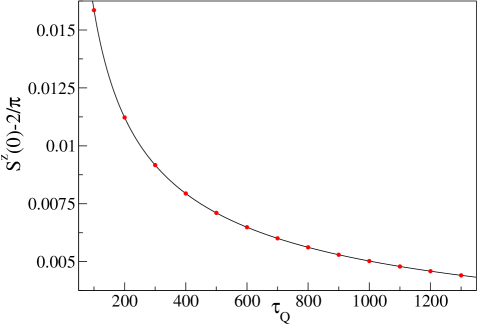
Figure 3: Non-equilibrium transverse magnetization at the critical point less the equilibrium value of this observable. We approximate the latter by $2/\pi$, which is the thermodynamic-limit result differing negligibly from the one that can be numerically obtained in the $N=1000$ system studied here. The black line comes from the fit $\ln(S^{z}(0)-2/\pi)=-1.8465(5)-0.4989(1)\ln(\tau_{Q})$. We report everywhere in this paper one standard error in the brackets next to the fitted coefficients.

Finally, anticipating discussion in Sec. IV, we introduce the transverse magnetization

$$S^{z}(t)=\langle\psi(t)|\sigma^{z}_{i}|\psi(t)\rangle=1-\frac{4}{N}\sum_{k}|v_{k}(t)|^{2}.$$ (48)

We are interested now in the value of this observable at time $t=0$, i.e., when the system arrives at the critical point. In the limit of $\tau_{Q}\to\infty$, $S^{z}(0)$ approaches the equilibrium value, which in the thermodynamically-large quantum Ising model at $g=1$ is equal to $2/\pi$. Our numerical simulations performed for $N\gg\hat{\xi}$, i.e. in the regime where the KZ theory is supposed to work, suggest that

$$S^{z}(0)-\frac{2}{\pi}\sim\frac{1}{\sqrt{\tau_{Q}}},$$ (49)

which is discussed in Fig. 3. A similar result is obtained when the continuous quench takes the Ising chain from one phase to another Pus .

IV Dynamics of the transverse magnetization at the critical point

After arriving at the critical point, the system undergoes free evolution. The wave-function is again given by (23). This time, however, the modes evolve according to

$$\mathrm{i}\frac{d}{dt}\left(\begin{array}[]{c}v_{k}\\ u_{k}\\ \end{array}\right)=\tilde{h}_{k}\left(\begin{array}[]{c}v_{k}\\ u_{k}\\ \end{array}\right),\ \tilde{h}_{k}=2\left(\begin{array}[]{cc}1-\cos(k)&-\sin(k)\\ -\sin(k)&\cos(k)-1\\ \end{array}\right).$$ (50)

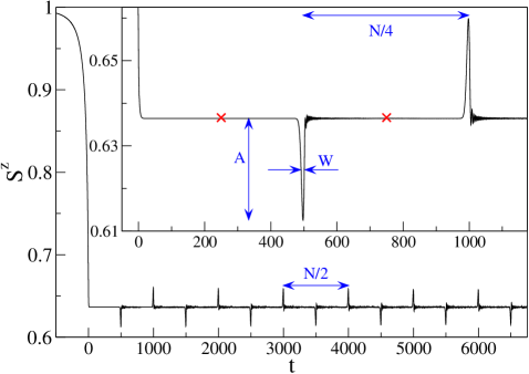
Figure 4: Dynamics of the transverse magnetization (48) for quench protocol (14). The inset zooms in the first two peaks that appear in the course of free evolution. Note that we do not count the decay of magnetization near $t=0$ as a peak. The amplitude and half-width of the first peak are marked as $A$ and $W$, respectively. The red crosses show the equilibrium value of the $S^{z}$ magnetization at the critical point of a thermodynamically-large system: $2/\pi\approx 0.637$. The system size $N=2000$ and the quench time $\tau_{Q}=100$.

Solving this equation with initial conditions that $v_{k}(0)$ and $u_{k}(0)$ are computed from (26) and (27), respectively, we get

$$\left(\begin{array}[]{c}v_{k}(t)\\ u_{k}(t)\\ \end{array}\right)=\left(\begin{array}[]{cc}\cos(\varepsilon_{k}t)-\mathrm{i}\sin(k/2)\sin(\varepsilon_{k}t)&\mathrm{i}\cos(k/2)\sin(\varepsilon_{k}t)\\ \mathrm{i}\cos(k/2)\sin(\varepsilon_{k}t)&\cos(\varepsilon_{k}t)+\mathrm{i}\sin(k/2)\sin(\varepsilon_{k}t)\\ \end{array}\right)\left(\begin{array}[]{c}v_{k}(0)\\ u_{k}(0)\\ \end{array}\right),$$ (51)

where

$$\varepsilon_{k}=4\sin(k/2).$$ (52)

Eigenvalues of the Hamiltonian $\tilde{h}_{k}$ are equal to $\pm\varepsilon_{k}$.

Having $v_{k}(t)$ modes, we can compute the transverse magnetization along the field direction (48)

$$S^{z}(t)=1-\frac{4}{N}\sum_{k}\!\left|[\cos(\varepsilon_{k}t)-\mathrm{i}\sin(k/2)\sin(\varepsilon_{k}t)]v_{k}(0)+\mathrm{i}\cos(k/2)\sin(\varepsilon_{k}t)u_{k}(0)\right|^{2}.$$ (53)

A typical result that we get is presented in Fig. 4, where both driven evolution to the critical point and free evolution at the critical point are plotted. We will focus on the latter below.

Figure 5: Illustration of quasi-periodicity of oscillations of the transverse magnetization at the critical point. Panels (a) and (b) show the amplitude and half-width of subsequent peaks–see Fig. 4. They show that peaks gradually become smaller in the amplitude and broader in the time domain. Panel (c) shows position in the time domain of subsequent peaks. The solid line is the linear fit $-2.66(4)+500.079(4)n$, where $n$ is the peak number. The distance between the peaks is nearly equal to $N/4=500$. It does not exhibit a gradual drift seen in panels (a) and (b). The plots are done for $N=2000$ and $\tau_{Q}=100$, just as in Fig. 4. The dots show numerics.

The main feature that we see in Fig. 4 is the series of quasi-periodic peaks in the transverse magnetization appearing during free evolution (we will call as peaks both minima and maxima, such as those separated by $N/4$ in the inset of Fig. 4). We use the term quasi-periodic to indicate that the width and amplitude of the peaks is not constant. This is illustrated in Fig. 5, where we see that the amplitude (width) of subsequent peaks is gradually decreasing (increasing). Note that the peaks appear at nearly identical time intervals.

To explain quasi-periodicity from Fig. 4, we note that after setting

$$\varepsilon_{k}\approx 2k$$ (54)

in (53), and using an expression for quasi-momenta (18), we get a periodic in time solution for $S^{z}(t)$ with the repetition period equal to $N/2$. Such an approximation is valid for small-momenta only, i.e., $k\ll\pi$. As a result, instead of a perfectly periodic pattern for $S^{z}(t)$, we get the quasi-periodic one. This can be understood in the following way. If we drove the system perfectly adiabatically to the critical point, we would see no oscillations of magnetization during free evolution as the system would be in the ground state. Oscillations that we see come from system excitation, which mainly affects the modes satisfying condition (34). For such modes approximation (54) is justified, leading to $N/2$ quasi-repetition period. This time scale is clearly associated with the characteristic time scale $\tau_{c}$ appearing at the critical point (11).

Next, we would like to understand how the width and amplitude of the peaks depend on the quench rate. As the analytical evaluation of (53) is impossible, we will again restore to an approximation. Namely, we will put expressions (36) and (37) into (53) and sum over all momenta (18). Such a procedure should reasonably account for the contribution of excited modes and ignore the contribution of the ones that evolved nearly adiabatically. The latter, however, do not contribute to the dynamics. In the end, keeping only the terms in the leading order in $k\sqrt{\tau_{Q}}$, we arrive at

$$S^{z}(t)\approx\text{const}-\frac{4}{N}\sum_{k}\!\left[\sin^{2}(\varepsilon_{k}t)+\frac{\sqrt{\pi}}{2}k\sqrt{\tau_{Q}}\sin(2\varepsilon_{k}t)+\frac{\pi}{2}k^{2}\tau_{Q}\cos^{2}(\varepsilon_{k}t)\right]e^{-\pi\tau_{Q}k^{2}/2},$$ (55)

where the constant term is time-independent. It does, however, depend on $\tau_{Q}$ due to (49).

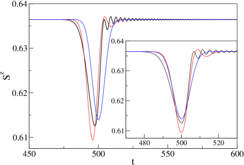
Figure 6: The first peak in the transverse magnetization during free time evolution. The black line shows numerics and comes from Fig. 4. The red line shows (55), while the blue line shows (58). The constant terms in (55) and (58) have been chosen to reproduce numerical results far away from the peak center. The inset shows the same as the main plot, but with data shifted horizontally so that the peaks are centered around the same time. The plots are done for $N=2000$ and $\tau_{Q}=100$.

The leading contribution in this expression comes from the zeroth-order term in $k\sqrt{\tau_{Q}}$, which we additionally simplify with (54) and identity $\sin^{2}(2kt)=1/2-\cos(4kt)/2$

$$S_{0}^{z}(t)=\text{const}+\frac{2}{N}\sum_{k}\cos(4kt)e^{-\pi\tau_{Q}k^{2}/2},$$ (56)

where $-2/N\sum_{k}e^{-\pi\tau_{Q}k^{2}/2}$ has been absorbed into the constant term. By putting quasi-momenta (18) into (56), we immediately see that its time-dependent component is anti-periodic with anti-period equal to $N/4$. This expression describes the peaks, whose width and shape can be obtained by replacement (43), which amounts to taking the thermodynamic limit. Doing so, one finds that the right-hand-side of (56) can be approximated for $\tau_{Q}\gg 1$ by

$$\text{const}+\frac{1}{\pi\sqrt{2\tau_{Q}}}e^{-8t^{2}/(\pi\tau_{Q})}.$$ (57)

The time-dependent part of such a result, however, is not anti-periodic because in the limit of $N\to\infty$ the anti-period of oscillations goes to infinity. The missing anti-periodicity can be recovered by writing the solution in the following form

$$S_{0}^{z}(t)=\text{const}+\frac{1}{\pi\sqrt{2\tau_{Q}}}\sum_{s=0}^{\infty}(-)^{s}e^{-8(t-sN/4)^{2}/(\pi\tau_{Q})}.$$ (58)

The differences between (56) and (58) are negligible when $N\gg 1$ and the width of the peaks is small compared to the period of oscillations. Approximations (55) and (58) are compared to numerics around the first peak in Fig. 6.

Using (58), one easily gets that the amplitude of the peaks is

$$A=\frac{1}{\pi\sqrt{2\tau_{Q}}}\approx\frac{0.225}{\sqrt{\tau_{Q}}},$$ (59)

while their half-width is

$$W=\sqrt{\frac{\pi\ln 2}{2}}\sqrt{\tau_{Q}}\approx 1.04\sqrt{\tau_{Q}}.$$ (60)

Several remarks are in order now.

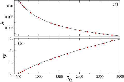
Figure 7: Properties of the first peak in the transverse magnetization as a function of the quench time $\tau_{Q}$. Panel (a): the amplitude of the first peak. Red dots show numerics, while the solid black line comes from the fit $\ln(A)=-1.421(2)-0.4962(3)\ln(\tau_{Q})$. This can be rewritten as $A\approx 0.241/\tau_{Q}^{0.496}$ and compared to (59). Panel (b): the half-width of the first peak. Again red dots show numerics, while the solid black line comes from the fit $\ln(W)=-0.05(3)+0.493(4)\ln(\tau_{Q})$, which can be reworked to $W\approx 0.951\tau_{Q}^{0.493}$ and compared to (60). The system size $N=2000$ in both panels.

First of all, it should be stressed that (58) is derived under approximation (54) and so its agreement with numerics should become gradually worse as time increases. Indeed, as we know from Fig. 5, the amplitude and half-width of the peaks varies in time in contrast to what (59) and (60) predict. Therefore, we will focus below on the discussion of how these two analytical predictions compare to numerics around the first peak, where our approximations should work best. Such numerics is discussed in Fig. 7. The $\tau_{Q}$ scaling exponents in (59) and (60) match it within about $1\%$, which is a very good result. The prefactors in (59) and (60) differ by about $8\%$ from the ones obtained numerically for the first peak, which is reasonable given the low order of the approximation.

Second, half-width (60) scales with $\tau_{Q}$ in the same way as $\hat{t}$ (see also discussion by the end of Sec. V). Thus, we see in the non-equilibrium dynamics at the critical point two characteristic time scales identified in Sec. I, $\hat{t}$ and $\tau_{c}$, that are given in the quantum Ising model by (11).

Third, we get by combining (59) and (60)

$$A\cdot W\approx 0.23,$$ (61)

which, quite interestingly, is $\tau_{Q}$-independent in the quantum Ising model. Nearly identical result can be obtained from the fits to numerical data discussed in Fig. 7.

Finally, we note that when the quench does not end at the critical point, different dynamics of the transverse magnetization during subsequent free evolution is observed Pus .

V The Loschmidt echo at the critical point

Using the results from Sec. IV, we can analyze the Loschmidt echo, which is defined here as the squared overlap between the initial state, say $|\phi\rangle$, and the time-evolved state, $e^{-\mathrm{i}\hat{\cal H}t}|\phi\rangle$. Such a quantity–also known as the return amplitude or fidelity–evolves in time whenever $|\phi\rangle$ is not an eigenstate of the Hamiltonian $\hat{\cal H}$. It has been recently intensively analyzed for sudden quenches, where $|\phi\rangle$ is an eigenstate of the pre-quench Hamiltonian, while $\hat{\cal H}$ is the post-quench Hamiltonian (see e.g. Hey (a); Car ; Naj for studies relevant to the quantum Ising model and Zvy ; Hey (b) for reviews).

We are interested in the Loschmidt echo at the critical point, $\hat{\cal H}=\hat{H}(g=1)$, computed for $|\phi\rangle$ being the non-equilibrium state of the quantum Ising model driven to the critical point

$$L(t)=|\langle\psi(0)|e^{-\mathrm{i}\hat{H}(g=1)t}|\psi(0)\rangle|^{2}=\!\left|\langle\psi(0)|\psi(t)\rangle\right|^{2},$$ (62)

where $|\psi(t)\rangle$ is obtained by combining (23) with (51). A similar strategy for studies of the Loschmidt echo in the quantum Ising model was employed in Pus , where a continuous quench starting and ending away from the critical point was used to prepare the state $|\phi\rangle$. This led to the dynamics of the Loschmidt echo, which differs from what we report below. We mention in passing that studies in Pus revolve around the aspects of the Loschmidt echo that are different from the ones we focus on.

Typical results that we obtain are presented in Fig. 8. Just as in Sec. IV, we observe peaks appearing at virtually identical time intervals (Fig. 9a), which become shorter and broader in the course of time evolution (Figs. 9b and 9c). The Loschmidt echo is nearly zero between the peaks. Analytical insights into some of the properties of the Loschmidt echo can be worked out in the following way.

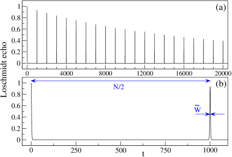
Figure 8: The Loschmidt echo for $N=2000$ spins and the quench time $\tau_{Q}=100$. Panel (a) illustrates periodicity and decay of echo revivals. Panel (b) shows the Loschmidt echo for small times up to the first peak. Note that we do not count the decay of the Loschmidt echo near $t=0$ as a peak. The half-width of the first peak is marked as $\tilde{W}$.

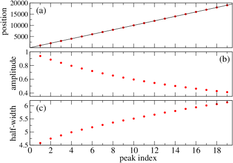
Figure 9: Illustration of quasi-revivals of the Loschmidt echo. Panel (a) shows position in the time domain of the subsequent peaks. The solid line is the linear fit $0.96(23)+1000.11(2)n$, where $n$ is the peak number. The distance between the peaks is nearly equal to $N/2=1000$. It does not exhibit a gradual drift with the peak number seen in panels (b) and (c) showing the amplitude and half-width of the subsequent peaks. These two panels show that the peaks gradually become smaller in amplitude and broader in the time domain. The plots are done for $N=2000$ and $\tau_{Q}=100$. The dots come from numerical simulations.

We use (23) and the normalization condition $|u_{k}(t)|^{2}+|v_{k}(t)|^{2}=1$ to find

$$L(t)=\prod_{k}\!\left(1-|u_{k}(0)v_{k}(t)-v_{k}(0)u_{k}(t)|^{2}\right).$$ (63)

Such an expression for $L(t)$ allows us to use approximations (36) and (37) for arbitrary $k$. Indeed, in the limit of small $k$, in the sense of (34), such approximations faithfully represent the exact result. In the opposite limit, due to the Gaussian cutoff (39) in (36) and (37), we are left in (63) with the product of unities representing the fact that large-enough $k$ Bogolubov modes do not get excited during time evolution towards the critical point. Such modes do not contribute to the Loschmidt echo. We note in passing that we compute the probability of finding the Ising chain in the ground state at $t=0$ through the product of $1-p_{k}$ in (30) due to exactly the same reasons.

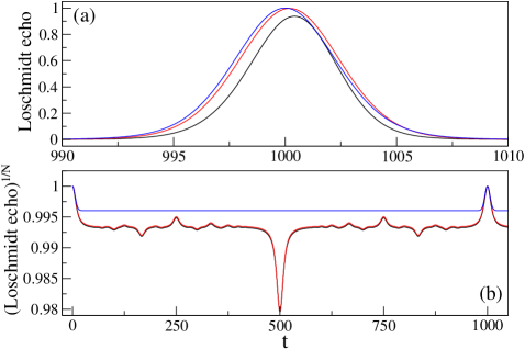
Figure 10: Panel (a) shows comparison between the exact numerical results for the Loschmidt echo near the first peak (black line) and approximations (64) and (68) given by the red and blue lines, respectively. Panel (b) shows data from panel (a) taken to the power of $1/N$ and displayed in a wider time range. In this way the Loschmidt echo between the peaks can be efficiently shown so that quality of the analytical approximations between the peaks can be critically assessed. The plots are done for $N=2000$ and $\tau_{Q}=100$.

Proceeding similarly as in Sec. IV, we arrive after expansion in $k\sqrt{\tau_{Q}}$ at

$$L(t)\approx\prod_{k}\!\left[1-\sin^{2}(\varepsilon_{k}t)e^{-\pi\tau_{Q}k^{2}}\right],$$ (64)

which can be compared to (55)–note that terms linear and quadratic in $k\sqrt{\tau_{Q}}$ vanish here. This can be further simplified by using (54) to get

$$L_{0}(t)=\prod_{k}\!\left[1-\sin^{2}(2kt)e^{-\pi\tau_{Q}k^{2}}\right],$$ (65)

which is periodic in time with period $N/2$. Next, in the spirit of the discussion from the previous section, we take the thermodynamic limit (43) on the right-hand-side of (65) to obtain

$$\exp\!\left(\frac{N}{2\pi}\int_{0}^{\pi}dk\ln\!\left[1-\sin^{2}(2kt)e^{-\pi\tau_{Q}k^{2}}\right]\right).$$ (66)

This can be further simplified by noting that the argument of the exponent is peaked around $t=0$, where it can be approximated by

$$-\frac{N}{2\pi}\int_{0}^{\pi}dk\sin^{2}(2kt)e^{-\pi\tau_{Q}k^{2}}\approx-\frac{N}{8\pi\sqrt{\tau_{Q}}}\!\left(1-e^{-4t^{2}/(\pi\tau_{Q})}\right)$$ (67)

for $\tau_{Q}\gg 1$. Restoring “by hand” $N/2$ periodicity, which we have lost by taking the thermodynamic limit in (66), we arrive at

$$L_{0}(t)\approx\exp\!\left[-\frac{N}{8\pi\sqrt{\tau_{Q}}}\!\left(1-\sum_{s=0}^{\infty}e^{-4(t-sN/2)^{2}/(\pi\tau_{Q})}\right)\right].$$ (68)

Several remarks are in order now.

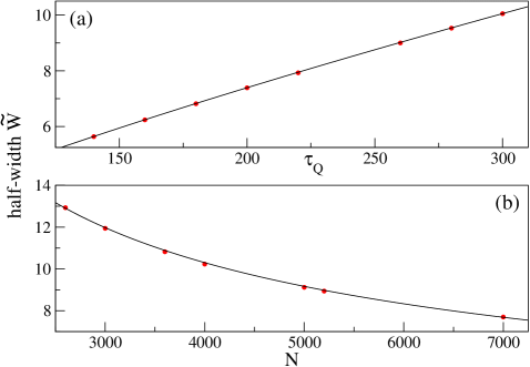
Figure 11: Panel (a): the half-width of the first peak of the Loschmidt echo for the system size $N=2000$. Solid black line comes from the fit $\ln(\tilde{W})=-2.01(1)+0.757(1)\ln(\tau_{Q})$, which can be rewritten as $\tilde{W}\approx 0.13\tau_{Q}^{0.757}$. This fit can be compared to (69) evaluated at $N=2000$, i.e., to $0.165\tau_{Q}^{3/4}$. Panel (b): the half-width of the first peak of the Loschmidt echo for the quench time $\tau_{Q}=500$. Solid black line comes from the fit $\ln(\tilde{W})=6.67(4)-0.523(5)\ln(N)$, which can be recast to $\tilde{W}\approx 788.4/N^{0.523}$. That fit can be compared to (69) after setting $\tau_{Q}=500$, which results in $\tilde{W}\approx 782.2/N^{1/2}$. Red dots depict numerics in both panels.

First, we would like to compare (64) and (68) to numerics for small times, where they should work best. Fig. 10a shows that around the maximum of the first peak both approximations provide similar results in reasonable agreement with numerics. Between the peaks, however, (64) significantly outperforms (68), which is shown in Fig. 10b. There is, in fact, quite a good agreement between (64) and numerics there. Thus, the dispersion relation (52) is the key to getting the numerous features of the Loschmidt echo between the peaks (similar features are seen in Fig. 2 of Car , where the Loschmidt echo for the sudden quench to the critical point is discussed).

Second, (68) predicts perfect revivals of the Loschmidt echo at time intervals equal to $N/2$. While such periodicity is clearly seen in the numerical data (Fig. 9a), the revivals that we observe are only partial (Fig. 9b).

Third, the half-width $\tilde{W}$ of the peaks of (68) is

$$\tilde{W}\approx\sqrt{-\pi\tau_{Q}\ln\!\left|1-\frac{8\pi\sqrt{\tau_{Q}}\ln 2}{N}\right|}\approx 2\pi\sqrt{2\ln 2}\frac{\tau_{Q}^{3/4}}{\sqrt{N}}\approx 7.4\frac{\tau_{Q}^{3/4}}{\sqrt{N}},$$ (69)

where condition (13) has been employed to simplify the logarithm. This result does not predict an increase of the half-width with peak index, which we see in Fig. 9c. Therefore, we will focus our attention on the half-width of the first peak, which we numerically study in Fig. 11. We see from the fits in this figure that the scaling exponents of (69) agree with numerics within a few percent, which is a very good result. The prefactor in (69) agrees with numerics to a lesser degree, i.e., within about $20\%$.

Dependence of $\tilde{W}$ on the quench time $\tau_{Q}$ and the system size $N$ is quite unusual at first glance. Working backwards through the calculation and restoring physical dimensions, we find that the right-hand-side of (69) can be written as

$$\tilde{W}\sim\hat{t}\sqrt{\frac{\hat{\xi}}{L}},$$ (70)

where $L$ is the system size equal to $N$ times the lattice constant. $L$ appears in (70) from changing the sum over momenta into the integral in (66). $\hat{\xi}$ comes from the Kibble-Zurek-like assumption that universal dynamics of the system depends on momenta through the $k/\hat{k}\sim k\hat{\xi}$ combination. Rescaling momenta under integral (67)

$$k\to k/\hat{\xi}$$ (71)

produces the $\hat{\xi}$ factor in (70). $\hat{t}$ enters (70) through the dispersion relation. To show this, we note that time enters our equations through $\varepsilon_{k}t\sim k^{z}t$ combination for low-energy modes at the critical point, whose excitation produces revivals in the Loschmidt echo. Then, we use rescaling (71) so that $\varepsilon_{k}t\to k^{z}t/\hat{\xi}^{z}$, and note that $\hat{\xi}^{z}\sim\hat{t}$ in the Kibble-Zurek theory. This produces $t/\hat{t}$ combination setting the time scale for (70).

Finally, we mention that similar reasoning can be used to argue that the half-width $W$ and amplitude $A$ of the peaks of transverse magnetization should scale in the quantum Ising model as $\hat{t}$ and $1/\hat{\xi}$, respectively. This observation agrees with the results reported in Sec. IV.

VI Summary

We have considered a continuous quench of the quantum Ising chain that was initially prepared in the ground state far away from the critical point in the paramagnetic phase. The quench has brought the chain to the critical point, where we have analytically determined how the probability of finding our system in the ground state depends on the quench rate. We have verified this result numerically and explained how it follows from the Kibble-Zurek theory of non-equilibrium phase transitions. In the context of the Kibble-Zurek theory, previous studies of the probability of finding the system in the ground state have been focused on quenches that ended far away from the critical point Jac (c); Mar ; BDp . Thus, our results provide complementary insights into the process of excitation during non-equilibrium phase transitions.

Next, we have focused our attention on the free evolution of such an out of equilibrium system at the critical point. We have numerically studied dynamics of its transverse magnetization and Loschmidt echo. We have found a series of quasi-periodic peaks in both observables and proposed a simple analytical model predicting some of their properties. In particular, such a model shows that the peaks should appear at time intervals proportional to the system size and that their width should scale with the quench rate in a way consistent with the Kibble-Zurek theory. These predictions have been compared to numerics for small times of free evolution and good overall agreement have been found.

It is perhaps worth to stress that our studies of dynamics of transverse magnetization did not employ the thermodynamic-limit approximation routinely used in the earlier works, see e.g. Bar ; Pus . This is important for two reasons. First, it allowed us to observe quasi-periodic peaks whose repetition period diverges in the thermodynamic limit. Second, finite-size results should be of experimental relevance in cold atom and ion quantum simulators, whose size is nowhere near the thermodynamic limit (see e.g. Luk ; Mon for fascinating recent experimental progress in studies of dynamics of quantum phase transitions).

We would also like to point that our studies of the Loschmidt echo at the critical point, unlike some former works Car ; Naj , involved a rather non-trivial initial state. Such a state was generated by the continuous quench imprinting universal critical exponents $z$ and $\nu$ onto the wave-function Jac (a); Dut ; Pol (a). This made the Loschmidt echo a richer object to study. Indeed, not only quantum revivals as in Car ; Naj can be studied in such a system, but also the details of the universal non-equilibrium dynamics.

Coming back to the discussion from Sec. I, we note that post-quench oscillations of magnetization at the critical point in the spin-1 Bose-Einstein condensate BDN and the quantum Ising model are quite different. Indeed, the period of such oscillations in the latter system is not only $\hat{t}$-independent but also divergent in the thermodynamic limit. Further studies are needed for explanation of this key difference.

Finally, we would like to mention two possible extensions of these studies. First, we believe that it would be interesting to find out if similar non-equilibrium dynamics can be observed in other integrable systems characterized by different critical exponents. Our preliminary results obtained for the Ising model with three-spin interactions Wol , where $z=2$ and $\nu=1$, show that magnetization rapidly oscillates during post-quench dynamics at the critical point instead of exhibiting distinct quasi-periodic peaks such as those illustrated in Fig. 4. Second, it would be also interesting to investigate the corresponding dynamics in near-integrable and non-integrable systems such as the Ising model in the transverse and longitudinal fields Col , the Bose-Hubbard model Lew ; Kru , the Dicke model Gar , etc. As all these experimentally-accessible systems undergo a quantum phase transition, their Kibble-Zurek dynamics at the critical point can be studied. Such dynamics, however, is expected to be considerably more complicated than that of integrable models (see Lan for a recent review on the relaxation dynamics of near-integrable systems).

References

- Jac (a) J. Dziarmaga, Adv. Phys. 59, 1063 (2010).
- (2) A. Dutta, G. Aeppli, B. K. Chakrabarti, U. Divakaran, T. F. Rosenbaum, and D. Sen, Quantum Phase Transitions in Transverse Field Spin Models: From Statistical Physics to Quantum Information (Cambridge University Press, 2015); arXiv:1012.0653.
- Pol (a) A. Polkovnikov, K. Sengupta, A. Silva, and M. Vengalattore, Rev. Mod. Phys. 83, 863 (2011).
- BDP (a) B. Damski, Phys. Rev. Lett. 95, 035701 (2005).
- (5) W. H. Zurek, U. Dorner, and P. Zoller, Phys. Rev. Lett. 95, 105701 (2005).
- Jac (b) J. Dziarmaga, Phys. Rev. Lett. 95, 245701 (2005).
- (7) T. W. B. Kibble, Phys. Rep. 67,183 (1980).
- (8) W. H. Zurek, Phys. Rep. 276, 177 (1996).
- del (a) A. del Campo, T. W. B. Kibble, and W. H. Zurek, J. Phys.: Condens. Matter 25, 404210 (2013).
- del (b) A. del Campo and W. H. Zurek, Int. J. Mod. Phys. A 29, 1430018 (2014).
- Pol (b) A. Polkovnikov, Phys. Rev. B 72, 161201(R) (2005).
- (12) S. Mostame, G. Schaller, and R. Schützhold, Phys. Rev. A 76, 030304(R) (2007).
- Pol (c) R. Barankov and A. Polkovnikov, Phys. Rev. Lett. 101, 076801 (2008).
- Sen (a) S. Mondal, K. Sengupta, and D. Sen, Phys. Rev. B 79, 045128 (2009).
- San (a) D. Patanè, L. Amico, A. Silva, R. Fazio, and G. E. Santoro, Phys. Rev. B 80, 024302 (2009).
- Jac (c) L. Cincio, J. Dziarmaga, J. Meisner, and M. M. Rams, Phys. Rev. B 79, 094421 (2009).
- Sen (b) K. Sengupta and D. Sen, Phys. Rev. A 80, 032304 (2009).
- Arn (a) A. Das, Phys. Rev. B 82, 172402 (2010).
- (19) M. Kolodrubetz, B. K. Clark, and D. A. Huse, Phys. Rev. Lett. 109, 015701 (2012).
- (20) A. Francuz, J. Dziarmaga, B. Gardas, and W. H. Zurek, Phys. Rev. B 93, 075134 (2016).
- San (b) A. Russomanno, S. Sharma, A. Dutta, and G. E. Santoro, J. Stat. Mech. (2015) P08030.
- (22) T. Puskarov and D. Schuricht, SciPost Phys. 1, 003 (2016).
- (23) S. Lorenzo, J. Marino, F. Plastina, G. M. Palma, and T. J. G. Apollaro, Sci. Rep. 7, 5672 (2017).
- Sen (c) K. Sengupta, S. Powell, and S. Sachdev, Phys. Rev. A 69, 053616 (2004).
- Cal (a) P. Calabrese, F. H. L. Essler, and M. Fagotti, J. Stat. Mech. (2012) P07016.
- Cal (b) P. Calabrese, F. H. L. Essler, and M. Fagotti, J. Stat. Mech. (2012) P07022.
- Arn (b) S. Bhattacharyya, A. Das, and S. Dasgupta, Phys. Rev. B 86, 054410 (2012).
- (28) R. Dorner, J. Goold, C. Cormick, M. Paternostro, and V. Vedral, Phys. Rev. Lett. 109, 160601 (2012).
- (29) F. H. L. Essler, S. Evangelisti, and M. Fagotti, Phys. Rev. Lett. 109, 247206 (2012).
- Hey (a) M. Heyl, A. Polkovnikov, and S. Kehrein, Phys. Rev. Lett. 110, 135704 (2013).
- Arn (c) S. Bhattacharyya, S. Dasgupta, and A. Das, Sci. Rep. 5, 16490 (2015).
- (32) B. Damski and W. H. Zurek, New J. Phys. 10, 045023 (2008).
- (33) E. Lieb, T. Schultz, and D. Mattis, Ann. Phys. (N.Y.) 16, 407 (1961).
- (34) P. Pfeuty, Ann. Phys. 57, 79 (1970).
- (35) B. Damski and M. M. Rams, J. Phys. A 47, 025303 (2014).
- (36) E. T. Whittaker and G. N. Watson, A Course of Modern Analysis (Cambridge University Press, Cambridge, England, 1958).
- BDP (b) B. Damski and W. H. Zurek, Phys. Rev. A 73, 063405 (2006).
- (38) P. Zanardi and N. Paunković, Phys. Rev. E 74, 031123 (2006).
- (39) S.-J. Gu, Int. J. Mod. Phys. B 24, 4371 (2010).
- (40) M. M. Rams and B. Damski, Phys. Rev. A 84, 032324 (2011).
- (41) B. Damski, Fidelity approach to quantum phase transitions in quantum Ising model, in Quantum Criticality in Condensed Matter: Phenomena, Materials and Ideas in Theory and Experiment, edited by J. Jedrzejewski (World Scientific, Singapore, 2015), pp. 159–182; arXiv:1509.03051.
- (42) M. M. Rams and B. Damski, Phys. Rev. Lett. 106, 055701 (2011).
- (43) J. Cardy, Phys. Rev. Lett. 112, 220401 (2014).
- (44) K. Najafi and M. A. Rajabpour, Phys. Rev. B 96, 014305 (2017).
- (45) A. A. Zvyagin, Low Temp. Phys. 42, 971 (2016).
- Hey (b) M. Heyl, Rep. Prog. Phys. 81, 054001 (2018).
- (47) E. Barouch, B. M. McCoy, and M. Dresden, Phys. Rev. A 2, 1075 (1970).
- (48) H. Bernien et al., Nature 551, 579 (2017).
- (49) J. Zhang et al., Nature 551, 601 (2017).
- (50) M. M. Wolf, G. Ortiz, F. Verstraete, and J. I. Cirac, Phys. Rev. Lett. 97, 110403 (2006).
- (51) R. Coldea et al., Science 327, 177 (2010).
- (52) M. Lewenstein, A. Sanpera, and V. Ahufinger, Ultracold Atoms in Optical Lattices: Simulating Quantum Many-Body Systems (Oxford University Press, Oxford, UK, 2012).
- (53) K. V. Krutitsky, Phys. Rep. 607, 1 (2016).
- (54) B. M. Garraway, Phil. Trans. R. Soc. A 369, 1137 (2011).
- (55) T. Langen, T. Gasenzer, and J. Schmiedmayer, J. Stat. Mech. (2016) 064009.