Enhancing Favorable Propagation in Cell-Free Massive MIMO Through Spatial User Grouping

Abstract

Cell-Free (CF) Massive multiple-input multiple-output (MIMO) is a distributed antenna system, wherein a large number of back-haul linked access points randomly distributed over a coverage area serve simultaneously a smaller number of users. CF Massive MIMO inherits favorable propagation of Massive MIMO systems. However, the level of favorable propagation which highly depends on the network topology and environment may be hindered by user’ spatial correlation. In this paper, we investigate the impact of the network configuration on the level of favorable propagation for a CF Massive MIMO network. We formulate a user grouping and scheduling optimization problem that leverages users’ spatial diversity. The formulated design optimization problem is proved to be NP-hard in general. To circumvent the prohibitively high computational cost, we adopt the semidefinite relaxation method to find a sub-optimal solution. The effectiveness of the proposed strategies is then verified through numerical results which demonstrate a non-negligible improvement in the performance of the studied scenario.

I Introduction

Recently, cell-free (CF) massive multiple-input multiple-output (MIMO) systems have attracted a lot attention [1, 2, 3] and have been recognized as an effective and appealing approach for next generation wireless networks. CF massive MIMO systems consist of very large number of single-antenna distributed access-points (APs) serving simultaneously, over same time/frequency resources, a relatively small number of users [2]. CF massive MIMO improves considerably macro-diversity and provides the network with substantially higher coverage probability.

CF massive MIMO can rely on channel reciprocity and uplink training in order to acquire channel state information (CSI) by adopting time-division duplex (TDD) mode [2]. With a large number of APs, CF massive MIMO can exploit favorable propagation that results from mutual orthogonality of users’ channel [4]. In [2], the authors leveraged favorable propagation to derive closed-form expressions for the downlink and uplink achievable rates for CF massive MIMO systems. The spatial correlation resulting from the distributed deployment of APs may however have a detrimental impact on the favorable propagation. More specifically, users that are relatively closed to each other will incur high spatial correlation which will jeopardize the mutual orthogonality of the users’ channel.

Channel hardening and favorable propagation in CF massive MIMO using stochastic geometry model were investigated in [5]. Therein, the authors concluded that one may not completely rely on channel hardening and favorable propagation when assessing the system’ performance since the derived bounds may not be tight due to the impact of spatial correlation between some users. Consequently, improving favorable propagation in presence of distributed antennas systems is of great necessity.

In this work, we analyze how spatial correlation between users’ channels vector influences favorable propagation and explore how to improve orthogonality between users’ channel by taking into account solely the large-scale fading and the number of available APs. We establish a design optimization problem based on the perspective of user’s scheduling. The proposed design advocates how users’ grouping can improve favorable propagation. However, the resulting optimization problem is difficult to solve in general. We demonstrate that the formulated problem is NP-hard and we invoke semidefinite relaxation (SDR) [6] approach to design a polynomial time solvable randomized procedure to find a sub-optimal solution to the NP-hard problem. In addition to that, to increase users’ throughput, we investigate the problem of bandwidth allocation for the resulting scheduling design strategy. The numerical results demonstrate that considerable performance improvement is achieved through the proposed efficient user grouping procedure and the bandwidth allocation scheme.

II System Model And Preliminaries

We consider a CF massive MIMO system that consists of of $K$ single omni-directional antenna users that are served simultaneously by $M$ single antenna APs. In this work, It is assumed that $K<<M$ and that the APs are using the same time-frequency resources. APs are randomly located within a given coverage area and are managed by a central processing unit (CPU) to which they are connected through perfect back-haul links. The CPU handles part of the physical layer processing such as data coding and decoding. Let $\bm{g}_{k}\in\mathbb{C}^{M\times 1}$, denote the complex channel vector between user $k$ and all the APs. Specifically, the $m$-th element, $g_{mk}$ is the channel coefficient between the $k$-th user and the $m$-th AP and is modeled as follows:

$$g_{mk}=\sqrt{\beta_{mk}}h_{mk}$$ (1)

where $h_{mk}\sim\mathcal{C}\mathcal{N}(0,1),m=1,\cdots,M,\quad k=1,\cdots,K,$ denote the small-scale fading coefficients which are independent and identically distributed (i.i.d) while $\beta_{mk},m=1,\cdots,M,\quad k=1,\cdots,K,$ the large scale fading coefficients that include path-loss and shadowing.

Similarly to the work done in [2], we assume uplink/downlink channels reciprocity. Provided that the system operates according to a TDD protocol, each coherence interval is divided between uplink training, downlink and uplink data transmission. In order to perform multiplexing and de-multiplexing, the APs need to acquire CSI through uplink training. Let $T_{c}$ be the length of the coherence interval (measured in samples) and $\tau$, the uplink training duration with $\tau<T_{c}$. During the uplink training phase, a maximum of $\tau$ users simultaneously send their pilot sequences to the APs. Under such setting, we consider a set of orthonormal training sequences, denoted by $\mathbf{q}_{k}\in\mathbb{C}^{\tau\times 1},\forall k=1,\cdots,\tau$ such that $\mathbf{q}^{\dagger}_{k}\mathbf{q}_{j}=\delta_{kj}$ (with $\delta_{kj}$ be the Kronecker delta).

Channel estimation is performed in a decentralized fashion where each AP $m$ independently estimates $g_{mk}$ of the $\tau$ active users. The received pilot vector signal at the $m$th AP can be expressed as

$$\bm{y}_{m,p}=\sqrt{\rho_{p}}\sum\limits_{k=1}^{\tau}g_{mk}\mathbf{q}_{k}+\bm{n}_{m,p}$$ (2)

where $\rho_{p}$ is the transmit power during the training phase and $\bm{n}_{m,p}$ is the additive Gaussian noise vector at the $m$-th AP. The elements of $\bm{n}_{m,p}$ are i.i.d. random variables. The $m$-th AP performs minimum mean-square error (MMSE) channel estimation using $\bm{y}_{m,p}$ in order to obtain the channel estimates given by

$$\hat{g}_{mk}=\frac{\sqrt{\rho_{p}}\beta_{mk}}{\rho_{p}\beta_{mk}+1}\big{(}\sqrt{\rho_{p}}g_{mk}+\bm{n}_{m,p}\mathbf{q}^{\dagger}_{k}\big{)},\,k=1,\cdots,\tau$$ (3)

Since the pilot sequences are mutually orthogonal, there is no pilot contamination and the channel estimate of each user $k$ is independent of $g_{mj},\forall j\neq k$. Each AP independently estimates the channel for each active user and the channel estimate is then used to precode the downlink signal. As in [2], we assume that conjugate beamforming is employed to communicate with the active users. Consequently, the transmit signal of the $m$-th AP can be expressed as

$$y_{m,d}=\sqrt{\rho_{d}}\sum\limits_{k=1}^{\tau}\hat{g}^{*}_{mk}d_{k}$$ (4)

where $d_{k}$ with ${\mathbb{E}}\left[\lvert d_{k}\rvert^{2}\right]=1$, denotes the data symbol intended to user $k$ while $\rho_{d}$, the downlink transmit power. The received signal at the $k$-th user is then given by

$$r_{k,d}=\sqrt{\rho_{d}}\left(\sum\limits_{m=1}^{M}{g}_{mk}\hat{g}^{*}_{mk}d_{k}+\sum\limits_{m=1}^{M}\sum\limits_{j\neq k}^{\tau}{g}_{mk}\hat{g}^{*}_{mj}d_{j}\right)+n_{k,d},$$ (5)

where $n_{k,d}$ denotes the white additive Gaussian noise at user $k$. By assuming a large number of APs, users can detect their downlink data using only the channel statistics [2]. The resulting rate of a given user $k$ can be written as [7]

$$R_{k,d}=\mathcal{B}\big{(}1-\frac{\tau}{T_{c}}\big{)}\;\text{log}_{2}\left(1+\frac{\rho_{d}(\sum\limits_{m=1}^{M}\nu_{mk})^{2}}{\rho_{d}\sum\limits_{m=1}^{M}\sum\limits_{j=1}^{\tau}\nu_{mk^{\prime}}\beta_{mk}+1}\right)$$ (6)

where $\mathcal{B}$ denotes the bandwidth of the system and $\nu_{mk}\triangleq\frac{\rho_{p}\beta_{mk}^{2}}{1+\rho_{p}\beta_{mk}}$ is the variance of $\hat{g}_{mk}$, the MMSE estimate of the channel.

III Improving favorable propagation: which users can be active simultaneously?

Favorable propagation represents an important property in large antenna systems. It refers to the mutual orthogonality between users’ vector wireless channel. With favorable propagation, the overall system’ performance is guaranteed to be very appealing with simple linear processing [4] since the effect of interferences is considerably attenuated. To obtain favorable propagation, users’ channel vectors need to be mutually orthogonal, i.e

$$\bm{g}^{\dagger}_{k}\bm{g}_{j}=\left\{\begin{array}[]{ll}0&\mbox{if $k\neq j$,}\\ \lVert\bm{g}_{k}\rVert^{2}\neq 0&\mbox{otherwise, }\end{array}\right.$$ (7)

Practically, the condition in (7) cannot be exactly met, but it can be approximately achieved. This is the case when the number of antennas grows large and the channels are said to provide asymptotically favorable propagation. The asymptotically favorable propagation condition is stated as

$$\frac{\bm{g}^{\dagger}_{k}\bm{g}_{j}}{M}\longrightarrow 0,\;M\longrightarrow\infty\quad\text{for}\quad k\neq j,$$ (8)

By using the channels gain from each AP to the users, equation (8) can be equivalently rewritten as

$$\frac{\sum\limits_{m=1}^{M}\sqrt{\beta_{m,k}}\sqrt{\beta_{m,j}}h^{*}_{m,k}h_{m,j}}{M}\longrightarrow 0\quad\text{for}\quad k\neq j,$$ (9)

Contrarily to collocated massive MIMO systems, the large scale fading coefficients from each AP to a given user are different in a cell-free Massive MIMO network. Intuitively, this spatial diversity will have a considerable impact on the favorable propagation. Consequently, spatial channel correlation is an important parameter that need to be taken into consideration to improve favorable propagation in the system.

In a practical scenario, the number of APs can be made very large but cannot grow indefinitely. Provided that asymptotically favorable propagation is achieved when $M$ tends to infinity, the condition in (8) will not meet for practical scenario. Given that favorable propagation is important to achieve good performance of CF massive MIMO, we use a different perspective to make condition in (8) works for practical scenario. To do so, we leverage the complementary cumulative distribution function of the inner product between two given users’ channel

$$P_{\theta}=\mathbb{P}\left\{\frac{\bm{g}^{\dagger}_{k}\bm{g}_{j}}{M}\geq\theta\right\}$$ (10)

Concretely, to improve favorable propagation, $P_{\theta}$ should be as close to zero as possible for any value of $\theta\geq 0$. Making $P_{\theta},\;\forall\theta\geq 0$ arbitrarily small means that the users’ channel vectors achieve near orthogonality. Using Chebychev’s inequality [8], $P_{\theta}$ can be lower-bounded by

$$P_{\theta}=\mathbb{P}\left\{\frac{\bm{g}^{\dagger}_{k}\bm{g}_{j}}{M}\geq\theta\right\}\leq\frac{1}{1+\frac{M^{2}\theta^{2}}{\sum\limits_{m=1}^{M}{\beta_{m,k}}{\beta_{m,j}}}},$$ (11)

From (11), it can be observed that a viable way to reduce the value of $P_{\theta}$, is to minimize the inner product between the users large scale fading vectors i.e., $\sum\limits_{m=1}^{M}{\beta_{m,k}}{\beta_{m,j}}$ which quantifies the spatial correlation between the channels of users $k$ and $j$. Consequently, reducing spatial correlation between active users’ channel in a CF massive MIMO system can considerably improve favorable propagation.

One plausible way to reduce spatial correlation is to resort to appropriate selection of active users. In this work, we construct a user’ scheduling optimization problem that enables users to be active simultaneously only when their channels have low spatial correlation. Our proposed scheme is discussed in the next section.

III-A Graphical Modeling and proposed solution

In the considered setting, the first step is to construct a spatial correlation graph that captures the level of favorable propagation for a set of users which are active simultaneously. More specifically, we design an undirected favorable propagation graph $\mathcal{G}(\mathcal{V},\mathcal{E})$. The set of of vertices $\mathcal{V}$ represents the users in the coverage area. Each edge $e_{k,j}\in\mathcal{E}$ is associated with a weight $\omega_{k,j}\triangleq\sum\limits_{m=1}^{M}\beta_{mk}\beta_{mj},$ which is directly related to the spatial correlation between the two users channel. Using the constructed graph $\mathcal{G}(\mathcal{V},\mathcal{E})$, we formulate a user selection optimization problem.

The considered optimization consists of minimizing the spatial correlation between the channels of users that belong to the same group. Consequently, we formulate a problem where we maximize the inter-group weights. The latter is equivalent to constructing groups with improved favorable propagation since users having high spatial correlation between their channels will be allocated to different groups. It is worth mentioning that the resulting uplink training overhead should be taken into account in the formulated optimization problem. To this end, the cardinality of each group should not violate a certain threshold so that CSI estimation can be performed without pilot contamination with a maximum training sequence of length $\tau$. Moreover, to fully exploit spatial diversity, a given user is allowed to belong to multiple groups simultaneously.

Define the following variable

$$x_{k,c}=\left\{\begin{array}[]{ll}1&\mbox{if user $k$ is allocated to the $c$-th group}\\ 0&\mbox{otherwise}\end{array}\right.$$ (12)

The user scheduling problem is formulated as the following combinatorial optimization problem

$$\max_{\begin{subarray}{c}x_{k,c}\in\{0,1\},\,\forall c,\forall k\end{subarray}}\leavevmode\nobreak \sum_{c=1}^{C}\sum_{k\in\mathcal{V}}\sum_{j\in\mathcal{V},j\neq k}w_{k,j}\left(1-x_{k,c}\right)x_{j,c}$$ (13)

s.t. $$\sum_{c=1}^{C}x_{k,c}\leq\alpha,\forall k\in\mathcal{V},$$

$$\sum_{k\in\mathcal{V}}x_{k,c}\leq\tau,\forall c=1,\ldots,C,$$

where $C$ denote the total number of groups and $\alpha$, the maximum number of groups to which a user can belong at the same time.

Before proceeding to solve problem (13), we investigate its computational tractability for $\alpha=1$. This is done through the following lemma.

Lemma 1.

Problem (13) is NP-hard in general.

Proof: We demonstrate the NP-hardness of problem (13) by considering a special case of our setting. Specifically, we study the complexity of problem (13) for $\alpha=1$ and $C*\tau\geq K$. It refers to the case where each user is allocated, at most, to one group and the constraints allow each users to be allocated at least once. The goal is to build the equivalence between this special case and the problem of partition into cliques of bounded size which is defined as follow [9]:

Definition 1.

Consider a graph $\mathcal{G}(\mathcal{V},\mathcal{E})$, a set function $f:2^{\mathcal{V}}\longrightarrow R^{+}$ and a bound $\tau\in Z^{+}$. The problem is to find a partition of the graph $\mathcal{G}$ into cliques $K_{1},...,K_{C}$ of size at most $\tau$, that is,$\lvert K_{c}\rvert\leq\tau,c=1,...,C$, such that the objective function $\sum_{c=1}^{C}f(K_{c})$ is minimized.

For $\alpha=1$, the maximization of the objective function of (13) is equivalent to maximizing $\sum_{c=1}^{C}\sum_{k\in\mathcal{V}}\sum_{j\in\mathcal{V},j\neq k}w_{k,j}-\sum_{c=1}^{C}\sum_{k\in\mathcal{V}}\sum_{j\in\mathcal{V},j\neq k}w_{k,j}x_{k,c}x_{j,c}$. As $C*\tau\geq K$, each user will be allocated to a given cluster. The first sum is then nothing but $2$ times the total weight between users. The considered optimization is then equivalent to minimizing $\sum_{c=1}^{C}\sum_{k\in\mathcal{V}}\sum_{j\in\mathcal{V},j\neq k}w_{k,j}x_{k,c}x_{j,c}$. Consequently, the simplified setting, with the cardinality constraints per group, is equivalent to solving a cardinality constrained graph partitioning into cliques that minimizes the sum of the clique functions given here by $\sum_{c=1}^{C}f(K_{c})=\sum_{c=1}^{C}\sum_{k\in\mathcal{V}}\sum_{j\in\mathcal{V},j\neq k}w_{k,j}x_{k,c}x_{j,c}$.

In graph theory, a clique is a subset of vertices of an undirected graph with complete induced subgraph. The aim of the problem given in Definition (1) is to partition the graph into cliques $K_{1}..K_{C}$ of maximum size $\tau$ such that the sum of the cost function over the cliques is minimized. The cost function in our case is given by the sum of the edges’ weights that have both their endpoints in the same cliques. Cardinality constrained graph partitioning into cliques with cost minimization contains the classic NP-hard clique cover problems. It is known as an NP-hard problem even with a submodular cost function in complete graphs [9]. Considering that problem (13) is equivalent to solving a cardinality constrained graph partitioning into cliques with cost minimization on the complete graph of spatial correlation, we deduce that it is a NP-hard problem.

One can prove the NP-hardness of (13) by another method. In fact, we can show that for $\alpha=1$, (13) is equivalent to another NP-hard problem, namely the capacitated max-$C$-cut problem. We skip the details for brevity.

$\blacksquare$

Since problem (13) is NP-hard for alpha=1, its global optimal solution cannot be found by mean of polynomial time solvable algorithms. For the general case of problem (13), where $\alpha\neq 1$, we design here a low-complexity algorithm to find a local optimal solution to problem (13). To do so, we will resort to semidefinite programming [10].

Define following variables and changes of variables

$$\mathbf{x}_{c}\leavevmode\nobreak \triangleq\left(x_{1,c}\cdots,x_{K,c}\right)^{\top},\,\mathbf{y}_{c}\triangleq 2\mathbf{x}_{c}-\mathbf{1}_{K}$$ (14)

$$\mathbf{W}\leavevmode\nobreak \triangleq\begin{pmatrix}0&w_{2,1}&\cdots&w_{K,1}\\ w_{1,2}&0&\cdots&w_{K,2}\\ \vdots&\vdots&\ddots&\vdots\\ w_{1,K}&w_{2,K}&\cdots&0\\ \end{pmatrix}$$

where $\mathbf{1}_{K}$ is a column vector which entries are $1$. Using (14), problem (13) can be equivalently reformulated as

$$\max_{\begin{subarray}{c}\end{subarray}}\leavevmode\nobreak\ \frac{1}{4}\sum_{c=1}^{C}\left(\varsigma-\mathbf{y}_{c}^{\top}\mathbf{W}\mathbf{y}_{c}\right)$$ (15a)

s.t. $$\sum_{c=1}^{C}\mathbf{y}_{c}\leq\bar{\alpha}$$ (15b)

$${\mathrm{Tr}}\left(\mathrm{diag}\left(\mathbf{y}_{c}\right)\right)\leq\bar{\tau},\,\forall c$$ (15c)

$$\mathbf{y}_{c}\in\{-1,1\}^{K},\forall c$$ (15d)

where $\varsigma=\mathbf{1}_{K}^{\top}\mathbf{W}\mathbf{1}_{K},\,\bar{\alpha}=2\alpha-C,\,\bar{\tau}=2\tau-K$. The proposed method consists of combining the semidefinite relaxation method [6] with the Schur complement [11]. More specifically, the quadratic terms $\mathbf{y}_{c}^{\top}\mathbf{W}\mathbf{y}_{c}={\mathrm{Tr}}\left(\mathbf{W}\mathbf{y}_{c}\mathbf{y}_{c}^{\top}\right),\,\forall c$ of the optimization problem (13) is approximated by the linear terms ${\mathrm{Tr}}\left(\mathbf{W}\mathbf{\text{Y}}_{c}\right),\,\forall c$ with the rank-one matrices $\mathbf{y}_{c}\mathbf{y}_{c}^{\top},\,\forall c$ being replaced by positive semidefinite matrices $\mathbf{\text{Y}}_{c},\,\forall c$ of arbitrary rank. The approximated problem is therefore formulated as

$$\max_{\begin{subarray}{c}\mathbf{\text{Y}}_{c}\succeq 0,\,\forall c\end{subarray}}\leavevmode\nobreak \frac{1}{4}\sum_{c=1}^{C}\left(\varsigma-{\mathrm{Tr}}\left(\mathbf{W}\mathbf{\text{Y}}_{c}\right)\right)$$ (16)

s.t. $$\sum_{c=1}^{C}\mathbf{y}_{c}\leq\bar{\alpha}$$

$${\mathrm{Tr}}\left(\mathrm{diag}\left(\mathbf{y}_{c}\right)\right)\leq\bar{\tau},\,\forall c$$

$$\mathrm{diag}\left(\mathbf{\text{Y}}_{c}\right)=\mathbf{1}_{K}$$

$$\begin{pmatrix}\mathbf{\text{Y}}_{c}&\mathbf{y}_{c}\\ \mathbf{y}_{c}^{\top}&1\end{pmatrix}\quad\succeq 0,\,\forall c$$

Problem (16) is a standard convex optimization problem and can be efficiently solved using interior-point based solvers such as CVX [12]. Since the optimization problem (16) is a relaxation of problem (15), the optimal $\mathbf{\text{Y}}_{c}^{\star},\,\forall c$ may not be of rank one. Hence, we resort to a randomized procedure, in the vein of Gaussian randomization [6], to convert the optimal solution of (16) into a feasible solution to problem (15). The proposed randomized scheme is summarized in Algorithm 1

1:  input an optimal solution $\mathbf{\text{Y}}_{c}^{\star},\,\forall c$ to problem (16).

2:  Generate $\bm{\xi}_{c}\sim\mathcal{N}(\bm{0},\mathbf{\text{Y}}_{c}^{\star}),\,\forall c$;

3:  Set $\widetilde{\bm{\xi}_{c}}=\bm{\xi}_{c}/{\mathrm{Tr}}\left(\mathrm{diag}\left(\bm{\xi}_{c}\right)\right),\,\forall c$;

4:  Generate $L$ vector samples $\widetilde{\mathbf{y}}_{c}^{l},\,l=1,\cdots,L$ feasible for problem (15) such that each entry $\widetilde{y}^{l}_{k,c},\,k=1,\cdots,C$ is drawn from the following distribution:

$$\widetilde{y}_{k,c}^{l}=\left\{\begin{array}[]{ll}1&\mbox{with probability $(1+\widetilde{\xi}_{k,c})/2$}\\ -1&\mbox{with probability $(1-\widetilde{\xi}_{k,c})/2$}\end{array}\right.$$ (17)

5:  Compute $l^{\star}=\arg max_{l=1,\cdots,L}\frac{1}{4}\sum_{c=1}^{C}\left(\varsigma-\left(\widetilde{\mathbf{y}}_{c}^{l}\right)^{\top}\mathbf{W}\widetilde{\mathbf{y}}_{c}^{l}\right)$;

6:  output the solution $\widehat{\mathbf{y}}_{c}=\widetilde{\mathbf{y}}_{c}^{l^{\star}},\,\forall c$.

Algorithm 1 A randomized algorithm to solve problem (15)

III-B Bandwidth allocation problem

Once a solution to problem (15) is found, we proceed to investigate the problem of bandwidth allocation. We denote $\Gamma(c)$, the set of users that belong to group $c$. Each group will be active over the assigned spectrum. The problem is formulated as

$$\max_{\begin{subarray}{c}0\leq\gamma_{c}\leq 1,\,\forall c\end{subarray}}\leavevmode\nobreak \sum_{c,k\in{\Gamma}(c)}\gamma_{c}\widetilde{R}_{k,c}$$ (18)

s.t. $$\overline{R}_{k}\leq\sum_{c=1}^{C}\gamma_{c}\widetilde{R}_{k,c},\forall k$$

$$\sum_{c=1}^{C}\gamma_{c}\leq 1$$

where ${\small{\widetilde{R}_{k,c}\triangleq\mathcal{B}\frac{T_{c}-\lvert{\Gamma}(c)\rvert}{T_{c}}\;\text{log}_{2}\left(1+\frac{\rho_{d}(\sum\limits_{m=1}^{M}\nu_{mk})^{2}}{\rho_{d}\sum\limits_{m=1}^{M}\sum\limits_{\begin{subarray}{c}k^{\prime}\in\Gamma(c)\\ k^{\prime}\neq k\end{subarray}}^{\tau}\nu_{mk^{\prime}}\beta_{mk}+1}\right)}}$ is the rate of the $k$th user within group $c$. And, $\overline{R}_{k}$ is the minimum rate requirements for the $k$th user. Problem (18) is a convex linear optimization problem and the optimal solution can be found using the interior-point method [11].

IV Numerical results

In this section, numerical results are provided in order to assess the performance of the proposed schemes. We consider a circular region having an area of $1\;\text{Km}^{2}$ where $M$ APs and $K$ users are randomly located according to a uniform distribution. The large-scale fading coefficients include the impact of the path loss, which is computed using a three slope path loss model [7], and log-normal shadow fading with standard deviation $\sigma_{sh}$. The large-scale fading coefficient $\beta_{mk}$ from user $k$ and AP $m$ is given by

$$\beta_{mk}=\left\{\begin{array}[]{ll}&(-L-35\;\text{log}_{10}(r_{mk}))\times SF_{mk},\;\mbox{if $r_{mk}>d_{1}$,}\\ &(-L-15\;\text{log}_{10}(d_{1})-20\;\text{log}_{10}(r_{mk}))\times SF_{mk}\\ &\qquad\qquad\qquad\qquad\qquad\qquad\mbox{if $d_{0}\leq r_{mk}\leq d_{1}$, }\\ &(-L-15\;\text{log}_{10}(d_{1})-20\;\text{log}_{10}(d_{0}))\times SF_{mk}\\ &\qquad\qquad\qquad\qquad\qquad\qquad\qquad\mbox{if $r_{mk}<d_{0}$. }\\ \end{array}\right.$$ (19)

where $SF_{mk}$ denotes the log-normal shadow fading between user $k$ and AP $m$ and $L$ is a constant depending on the carrier frequency, the user and AP heights. All other simulation parameters are summarized in Table I. The performance of the proposed scheme is compared with the approach provided in [2] but with uniform power allocation (we refer to this scheme as conventional CF).

Carrier frequency	$1.9\;\text{GHz}$	Bandwidth	$20\;\text{MHz}$
Noise figure	$9\;\text{dB}$	AP antenna height	$15\;\text{m}$
$\sigma_{sh}$	$8\;\text{dB}$	User antenna height	$1.7\;\text{m}$
$T_{c}$	$200$	$\rho_{d},\rho_{p}$	$200,150\;\text{mW}$

Table I: Simulation parameters

Figure 1: Comparison of CDFs of normalized large-scale fading correlation for $K=20,\alpha=6,C=4$

Figure 1 shows the impact of the proposed spatial grouping (SG) on the normalized large-scale fading correlation for different values of $M$. We can see that appropriate spatial user grouping substantially reduces spatial correlation within each group which results in more favorable propagation. From Figure 1, we observe that SG enables to achieve, for $M=100$, spatial correlation levels comparable to conventional CF with $M=200$. This means that SG can be a very practical alternative to network densification.

Figure 2 exemplifies the average downlink net throughput versus the number of APs ($M$) for $K=10$ and $15$, respectively. Figure 2 demonstrates that the performance of both approaches improves as M increases. This is a direct consequence of array gain increase. In addition, Figure 2 also shows that the proposed SG with bandwidth allocation (BA) outperforms the conventional CF system. This is due to the fact that SG improves favorable propagation within each group. Indeed, SG enables gains of $18.5\%$ and $17.05\%$, for $(M=100,K=10)$ and $(M=100,K=15)$, respectively. Consequently, appropriate user grouping and selection can be a more practical and cost efficient alternative to increasing the number of APs. Indeed, for $K=15$, SG achieves approximately the same downlink throughput ( $14.956\;Mbits/s$) at $M=85$ as the conventional CF system with $M=100$.

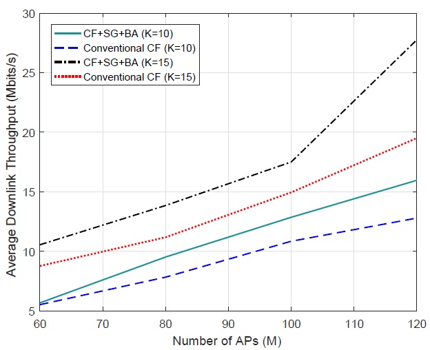
Figure 2: Average Downlink Throughput versus the number of APs and different K values ($\tau=K$)

V Conclusion

In this work, we investigated how favorable propagation can be improved in CF massive MIMO systems. We formulated an NP-hard spatial user grouping problem based on large-scale fading coefficients. We designed an SDR-based algorithm to find an efficient sub-optimal solution. Orthogonal frequency resources are also allocated to the spatial groups. The simulation results showed that reducing spatial correlation between active users through efficient spatial grouping considerably improves favorable propagation, increases the average throughout and enables to achieve better performance with lower numbers of APs.

References

- [1] E. Nayebi, A. Ashikhmin, T. L. Marzetta, and H. Yang, Cell-Free Massive MIMO systems, in 2015 49th Asilomar Conference on Signals, Systems and Computers, Nov 2015, pp. 695-699.
- [2] H. Q. Ngo, A. Ashikhmin, H. Yang, E. G. Larsson, and T. L. Marzetta, Cell-Free Massive MIMO Versus Small Cells, IEEE Transactions on Wireless Communications, vol. 16, no. 3, pp. 1834-1850, March 2017.
- [3] E. Nayebi, A. Ashikhmin, T. L. Marzetta, H. Yang, and B. D. Rao, Precoding and Power Optimization in Cell-Free Massive MIMO Systems, IEEE Transactions on Wireless Communications, vol. 16, no. 7, pp. 4445-4459, July 2017.
- [4] H. Q. Ngo, E. G. Larsson, and T. L. Marzetta, Aspects of favorable propagation in Massive MIMO, in 2014 22nd European Signal Processing Conference (EUSIPCO), Sept 2014, pp. 76-80.
- [5] Z. Chen and E. Bjornson, Channel hardening and favorable propagation in cell-free massive MIMO with stochastic geometry, CoRR, 2017.
- [6] Z. Q. Luo, W. K. Ma, A. M. C. So, Y. Ye, and S. Zhang, Semidefinite Relaxation of Quadratic Optimization Problems, IEEE Signal Processing Magazine, vol. 27, no. 3, pp. 20-34, May 2010.
- [7] H. Q. Ngo, L. N. Tran, T. Q. Duong, M. Matthaiou, and E. G. Larsson, On the Total Energy Efficiency of Cell-Free Massive MIMO, IEEE Transactions on Green Communications and Networking, vol. PP, no. 99, 2017.
- [8] W. Hoeffding, Probability Inequalities for Sums of Bounded Random Variables, Journal of the American Statistical Association, vol. 58, no. 301, pp. 13-30, 1963.
- [9] J. R. Correa and N. Megow, Clique partitioning with value-monotone submodular cost, Discrete Optimization, vol. 15, pp. 26-36, 2015.
- [10] L. Vandenberghe and S. Boyd, Semidefinite programming, SIAM Rev., vol. 38, no. 1, pp. 49-95, March 1996.
- [11] S. Boyd and L. Vandenberghe, Convex Optimization. Cambridge, U.K.: Cambridge Univ. Press, 2004.
- [12] M. Grant and S. Boyd, CVX: Matlab software for disciplined convex programming, version 2.1, http://cvxr.com/cvx, March 2014.