Approximation of quantum control correction scheme using deep neural networks

Abstract

We study the functional relationship between quantum control pulses in the idealized case and the pulses in the presence of an unwanted drift. We show that a class of artificial neural networks called LSTM is able to model this functional relationship with high efficiency, and hence the correction scheme required to counterbalance the effect of the drift. Our solution allows studying the mapping from quantum control pulses to system dynamics and analysing its behaviour with respect to the local variations in the control profile.

I Introduction

The main objective and motivation of quantum information processing is the development of new technologies based on principles of quantum mechanics such as superposition and entanglement Dowling and Milburn (2003). Quantum technologies require the development of methods and principles of quantum control, the control theory of the quantum mechanical system d’Alessandro (2007). Such methods have to be developed by taking into account the behaviour of quantum systems Gough and Belavkin (2013); Pawela and Puchała (2014). In particular, as quantum systems are very susceptible to noise, which may influence the results of the computation, the methods of quantum control have to include the means for counteracting the decoherence Viola and Lloyd (1998).

The presented work is focused on the development of tools suitable for analysing the relation between the control pulses used for idealized quantum systems, and the control pulses required to execute the quantum computation in the presence of undesirable dynamics. Modelling this relation is important to better understand the manifold of control pulses in the presence of noise, a case which is still poorly understood. We focus on quantum dynamics described by a quantum spin chain. We are interested in a method of approximating the correction function of normal control pulses (NCP), i.e. the function accepting control pulses corresponding to the system without the drift Hamiltonian and generating the de-noising control pulses (DCP) for the system with the drift Hamiltonian. The existence of this function is non-trivial, since there are infinitely many pulses that produce the same evolution. We propose an approximation that not only incorporates the global features of the function but also describes its local properties. This feature is in contrast with available methods based on optimisation which do not take into account the continuous behaviour of the map from NCP to the de-noising control pulses. Indeed, without further assumptions, in view of the non-injectivity of quantum control, we may expect no relation at all between control pulses obtained from the optimization of different problems. On the other hand, we show that machine learning methods can be used for this purpose.

Recently, significant research effort has been invested in the application of machine learning methods in quantum information processing Ciliberto et al. (2018); Dunjko and Briegel (2017); Ostaszewski et al. . In particular, optimization techniques borrowed from machine learning have been used to optimize the dynamics of quantum systems van Nieuwenburg et al. (2018), either for quantum control Zahedinejad et al. (2014); August and Hernández-Lobato (2018) and simulation Las Heras et al. (2016), or for implementing quantum gates with suitable time-independent Hamiltonians Banchi et al. (2016). These techniques include also quantum control techniques from dynamic optimization Sridharan et al. (2008) and reinforcement learning Bukov et al. (2017); Niu et al. (2018). In the presence of noise, neural networks give tools for optimizing dynamical decoupling, which can be seen as a quantum control correction scheme as considered by us, in a special case of the target operation being identity August and Ni (2017). On the level of gate decomposition, neural networks have also been applied to the problem of decomposing arbitrary operations as a sequence of elementary gate sets Swaddle et al. (2017); Fösel et al. (2018).

In this paper, we propose a method, based on an artificial neural network (ANN), to study the correction scheme between control pulses obtained in the ideal case, and those obtained when the system is subject to undesired dynamics. Moreover, we demonstrate that the utilized network has high efficiency and can be used to analysis of the properties of the model.

This paper is organized as follows. In Section II we introduce the model and describe the architecture of a deep neural network which will be used as an approximation function. In Section III we demonstrate that the proposed methods can be used for generating control pulses without the explicit information about the model of a quantum system. We also utilize it for the purpose of analysing the properties of the correction scheme. Section V contains summary of the presented results.

II Methods: Model and solution

In this section, we provide necessary notation and background information. We start by introducing a spin-chain model and describe the problem of generating quantum control pulses that counteract the undesired dynamics present in the system. We also introduce the architecture of the artificial neural network used to approximate the correction scheme.

II.1 Model of quantum system

Let us consider a system of two interacting qubits. The evolution of the system is described by GKSL master equation

$$\frac{\mathrm{d}\rho}{\mathrm{d}t}=-\mathrm{i}[H(t),\rho]+\sum_{j}\gamma_{j}(L_{j}\rho L_{j}^{\dagger}-\frac{1}{2}\{L_{j}^{\dagger}L_{j},\rho\}).$$ (1)

where the Hamiltonian has three components

$$H(t)=H_{c}(t)+H_{0}+H_{\gamma}.$$ (2)

We consider the control Hamiltonian of the form

$$H_{c}(t)=h_{x}(t)\sigma_{x}\otimes{\rm 1l}+h_{z}(t)\sigma_{z}\otimes{\rm 1l},$$ (3)

and the base Hamiltonian

$$H_{0}=\sigma_{x}\otimes\sigma_{x}+\sigma_{y}\otimes\sigma_{y}+\sigma_{z}\otimes\sigma_{z}.$$ (4)

The last element in Eq. (2) is the drift Hamiltonian, which can be an arbitrary two-qubit Hamiltonian multiplied by real parameter $\gamma>0$. Incoherent part of Eq. 1 models interaction with an environment with strengths $y_{j}$. It should be noted that in this paper will never consider the case when $\gamma$ and $\gamma_{j}$ both are different form zero.

Quantum optimal control refers to the task of executing a given unitary operation via the evolution of the system, in our case described by Eq. (2). To achieve this, one has to properly choose the coefficients $h(t)=(h_{x}(t),h_{z}(t))$ in Eq. (3). The set of reachable unitaries can be characterized d’Alessandro (2007) by studying the Lie algebra generated by the terms in Eq. (2). For $H_{\gamma}=0$ our system is fully-controllable, so any target can be obtained with suitable choice of $h(t)$, with no restriction on the control pulses. We assume that function $h(t)$ is piecewise constant in time slots $\Delta t_{i}=[t_{i},t_{i+1}]$, which are the equal partition of evolution time interval $T=\bigcup_{i=0}^{n-1}\Delta t_{i}$. We also assume that $h_{x}(t)$ and $h_{z}(t)$ have values from interval $[-1,1]$.

Function $h(t)$ will be represented as vectors of values of $h_{x}(t)$ and $h_{z}(t)$. For the case $\gamma=0$, we say that it represents NCP— normal control pulses. Alternatively, for $\gamma\neq 0$, we say that $h(t)$ represents DCP—de-noising control pulses. Since $h(t)$ is piecewise constant, both NCP and DCP have two indices, with first index corresponding to time slots $\{0,\ldots,n-1\}$, and the second index corresponding to the direction $\{x,z\}$, namely

$$\begin{split}NCP_{i,j}&=h_{j}(t),\ \gamma=0,\\ DCP_{i,j}&=h_{j}(t),\ \gamma\neq 0,\\ \end{split}$$ (5)

where

$$t\in[t_{i},t_{i+1}]\ i\in\{0,\ldots,n-1\},\ j\in\{x,z\}.$$ (6)

It is worth noting that the mapping from the set of control operations to the unitary operator is not injective. Namely the same unitary can be obtained using different choices of $h(t)$. To study the relationship between NCP and DCP we need to select the DCP which is more closely related to the NCP. Because of continuity, we do that numerically by using the NCP as starting guess of the DCP. The final optimal DCP is then found using a local optimisation around the initial NCP.

The figure of merit in our problem is the fidelity distance between superoperators, defined as Floether et al. (2012)

$$F=1-F_{err},$$ (7)

with

$$F_{err}=\frac{1}{2N^{2}}(\mathrm{Tr}(Y-X(T))^{\dagger}(Y-X(T))),$$ (8)

where $N$ is the dimension of the system in question, $Y$ is superoperator of the fixed target operator, and $X(T)$ is evolution superoperator of operator resulting from the numerical integration of Eq. (1) with given controls. In particular, for a target unitary operator $U$, its superoperator $Y$ is given by the formula

$$Y=U\otimes\bar{U}.$$ (9)

Superoperator $X(T)$ is obtained from the unitary operator resulting from the integration of the Eq. (1).

II.2 Architecture of artificial neural network

The control pulses used to drive the quantum system with Hamiltonian from Eq. 3 are formally a time series. This aspect suggests that one may study their properties using methods from pattern recognition and machine learning Bishop (1995); Goodfellow et al. (2016) that have been successfully applied to process data with similar characteristics. The mapping from NCP to DCP share similar mathematical properties with that of statistical machine translation Koehn (2009), a problem which is successfully modelled with artificial neural networks (ANN) Bahdanau et al. (2014). Because of this analogy, we use ANN as the approximation function to learn the correction scheme for control pulses. A trained artificial neural network will be used as a map from NCP to DCP

$$\textrm{ANN}(\textrm{NCP})=\textrm{nnDCP},$$ (10)

where nnDCP, neural network DCP, is an approximation of DCP obtained by using the neural network.

Because of time series character of control sequences, we utilize bidirectional long short-term memory (LSTM) networks Hochreiter and Schmidhuber (1997). The long short-term memory block is a special kind of recurrent neural network (RNN), a type of neural network with directed cycles between units. These cycles allow the RNN to keep track of the inputs received during the former times. In other words, the output at given time depends not only on current input, but also on the history of earlier inputs. This kind of neural networks is applicable in situations with time series with long-range correlations, such as in natural language processing where the next word depends on the previous sentence but also on the context.

Figure 1: Structure of LSTM network used in the experiments.

LSTM block consists of two cells

cell state

$c_{t}=c_{t-1}\circ\textrm{f}_{t}+\tilde{c}_{t}\circ\textrm{i}_{t},$

hidden state

$s_{t}=\tanh(c_{t})\circ\textrm{o}_{t},$

which are constructed from following gates

input gate

$\textrm{i}_{t}=\textrm{sigma}(x_{t}V^{\textrm{i}}+s_{t-1}W^{\textrm{i}}),$

forget gate

$\textrm{f}_{t}=\textrm{sigma}(x_{t}V^{\textrm{f}}+s_{t-1}W^{\textrm{f}}),$

output gate

$\textrm{o}_{t}=\textrm{sigma}(x_{t}V^{\textrm{o}}+s_{t-1}W^{\textrm{o}}),$

candidate

$\tilde{c}_{t}=\tanh(x_{t}V^{\textrm{o}}+s_{t-1}W^{\textrm{o}}),$

where $\circ$ is element wise multiplication of two vectors, $s_{t-1}$ is previous hidden state, and $x_{t}$ is an actual input state. Matrices $V$ and $W$ are the weight matrices of each gate. As one can see there is only one gate with hyperbolic tangent as activation function – candidate gate. Rest of the gates has sigmoid activation function which has values from $[0,1]$ interval. Using this function, neural networks decides which values are worth to keep and which should be forgotten. This gates maintain the memory of the network.

Basic architectures of RNN are not suitable for maintaining long time dependences, due to the so-called vanishing/exploding gradient problem – the gradient of the cost function may either exponentially decay or explode as a function of the hidden units. Thanks to the structure of LSTM the exploding gradient problem is reduced. The bidirectional version of LSTM is characterized by the fact that it analyses the input sequence/time series forwards and backwards. Thanks to this it uses not only information from the past but also from the future Schuster and Paliwal (1997); Graves et al. (2005). For this purpose the bidirectional LSTM unit consists of two LSTM units. One of them takes as an input vector $[h(t_{1}),h(t_{2}),\ldots,h(t_{n})]$, and the second takes $[h(t_{n}),h(t_{n-1}),\ldots,h(t_{1})]$.

As in Eq. (10), the result of the network is a vector of control pulses nnDCP. To evaluate the quality of nnDCP we apply loss function described in Eq. 8. To achieve this we integrate a new superoperator $X(T)$ form nnDCP and measure how far it is from the target superoperator $Y$.

For two-qubit systems, we found that three stacked bidirectional LSTM layers are sufficient for obtaining the high value of fidelity. Moreover, at the end of the network we use one dense layer which processes the output of stacked LSTM to obtain our nnDCP. Experiments are performed using TensorFlow library Abadi et al. (2016); ten .

III Results: Experiments

For the purpose of testing the proposed method we use a sample of Haar random unitary matrices Mezzadri (2007); Miszczak (2012). Pseudo-uniform random unitaries can be obtained also in the quantum control setting via random functions $h(t)$, provided that the control time $T$ is long enough Banchi et al. (2017). The exact implementation of sampling random Haar unitary matrices is available at qco . In our experiments we use QuTIP qut (012); Johansson et al. (2012, 2013) to generate control pulses to training and testing data. First, we construct the target operators

$$U_{target}=U\otimes{\rm 1l},$$ (11)

where $U\in\mathbf{U}(2)$ is a random matrix. Next, using QuTIP we generate NCP corresponding to the target operators. In the case of our setup, the parameters are fixed as follows:

• time of evolution $T=6$,

• number of intervals $n=32$,

• control pulses in $[-1,1]$.

We train the network using a subset of the generated pairs {(NCP, $Y_{target}$)}, where $Y_{target}$ is a target superoperator obtained from $U_{target}$. In the training process network takes NCP as input and generates the nnDCP. Next this nnDCP is an input to the loss function. For this purpose we construct superoperator $X(T)$ resulting from integration of Eq. (1) using nnDCP. Next, we calculate error function between $X(T)$ and $Y_{target}$ as in Eq. (8). In this section we analyse only coherent drift i.e. in Eq.(1) $\gamma_{j}=0$.

Source code implementing experiments described in this paper is available at qco .

III.1 Performance of the neural network

The first experiment is designed to analyse the efficiency of the trained network in terms of fidelity error of generated nnDCP control pulses. Trained LSTM have mean fidelity on the test set as presented in Table 1. It should be noted that, despite the fact that the mean fidelity on the test set is high, the trained network sometimes has outlier results i.e. it returns nnDCP which corresponds to the operator with high fidelity error.

	$\gamma$
$H_{\gamma}$	$0.2$	$0.4$	$0.6$	$0.8$
$\gamma(\sigma_{y}\otimes{\rm 1l})$	$.96$	$.92$	$.95$	$.96$
$\gamma(0.2\sigma_{x}\otimes{\rm 1l}+0.8\sigma_{y}\otimes{\rm 1l})$	$.97$	$.94$	$.97$	$.97$
$\gamma(0.5\sigma_{x}\otimes{\rm 1l}+0.5\sigma_{y}\otimes{\rm 1l})$	$.98$	$.96$	$.98$	$.97$
$\gamma(0.8\sigma_{x}\otimes{\rm 1l}+0.2\sigma_{y}\otimes{\rm 1l})$	$.99$	$.97$	$.98$	$.99$

Table 1: The average of mean fidelity score. For each Hamiltonian and each parameter $\gamma$, 10 independent experiments have been performed. It should be noted that first two columns with results i.e. comlums corresponding to $\gamma=0.2$ and $0.4$ are obtained from network which takes mini batches equal to 5 and 4000 training samples and 1000 testing samples. Next two columns i.e. $\gamma=0.6$ and $0.8$ are obtained from network with mini batches 50 and 8000 training samples and 4000 testing samples.

	$\gamma$
$H_{\gamma}$	$0.6$	$0.8$
$\gamma(\sigma_{y}\otimes\sigma_{y})$	$.98$	$.90$
$\gamma(0.1\sigma_{x}\otimes\sigma_{x}+0.8\sigma_{y}\otimes\sigma_{y}+0.1\sigma_{z}\otimes\sigma_{z})$	$.98$	$.98$
$\gamma(0.1\sigma_{x}\otimes\sigma_{x}+0.6\sigma_{y}\otimes\sigma_{y}+0.3\sigma_{z}\otimes\sigma_{z})$	$.98$	$.98$
$\gamma(0.2\sigma_{x}\otimes\sigma_{x}+0.6\sigma_{y}\otimes\sigma_{y}+0.2\sigma_{z}\otimes\sigma_{z})$	$.96$	$.97$
$\gamma(0.3\sigma_{x}\otimes\sigma_{x}+0.6\sigma_{y}\otimes\sigma_{y}+0.1\sigma_{z}\otimes\sigma_{z})$	$.98$	$.98$

Table 2: The average mean fidelity scores for spin chain drifts. This results are obtained for network with mini batch equal to 10 and 8000 training samples and 4000 testing samples.

The performed experiments show that it is possible to train LSTM networks for a given system with high efficiency. Results from Table I are obtained by trained artificial neural networks on different kinds of drift, i.e. $\alpha\sigma_{x}\otimes{\rm 1l}+(1-\alpha)\sigma_{y}\otimes{\rm 1l}$ for $\alpha\in\{0,0.2,0.5,0.8\}$, with different values of $\gamma$. The experiment with this kind of drift is representative because $\sigma_{y}$ is orthogonal to the controls $\sigma_{x},\sigma_{z}$. The performed experiment shows that it is possible to train LSTM to have the efficiency on the test set above $90\%$ for chosen gammas. Some of results from Table 1 have average score lower than $90\%$. This is caused by the outlier cases, when network performs with very low efficiency. Such efficiency for chosen gammas is sufficient to our goal, which is to study the relations between the system and control pulses for relatively small disturbances.

In Table 2 we present average score for model with spin chain drift. As one can see, these results are much better than in Table 1. This can be explained by the fact that this type of drift is similar to the base Hamiltonian $H_{0}$ which is also a spin chain.

Results from above tables may suggest the answer for non trivial questions: for what kind of drift, map between NCP and DCP is easier to learn. If training on the model with drift operating the same system as the control is easier than training on the model with drift similar to base Hamiltonian? Obtained results suggest that, when the drift is asymmetric with respect to the base Hamiltonian, the neural network requires larger mini batch sizes to achieve similar efficiency.

As one can see, the efficiency of the artificial neural networks depends on the choice of the hyperparameters. In our case, for some values of parameter $\gamma$ one needs to use bigger batch size and the larger training set to obtain satisfactory results. This behavior is incomprehensible because, for $\gamma=0.6$ and batch size equal to 5, RNN has problems with convergence. However, by increasing the batch size we were able to improve the performance. We would like to stress that our aim was to show that it is possible to obtain mean efficiency greater than 90%, not to examine what is the best possible efficiency of the network.

III.2 Utilization of the approximation

In this section, we show the results of an experiment, which allows checking what is the behaviour of the ANN() function when we perform local disturbances on a set of random NCP, and we check what is the deviation of the new nnDCP from the original DCP. The original DCP is obtained from GRAPE algorithm initialized by NCP.

Let us suppose that we have a trained LSTM. The procedure of checking its sensitivity on variations of $h_{j}(t)$, for $j\in\{x,z\}$ and $t$ in the $i$-th time slot, is as follows.

• Select a NCP vector from the testing set and generate the corresponding nnDCP.

• If the fidelity between target operator and operator resulting from nnDCP is lower than $90\%$ return to Step 1.

• Select $i\in\{0,\ldots,n-1\}$, $j\in\{x,z\}$, change $(i,j)$ coordinate of NCP by fixed $\varepsilon$

  • if $\textrm{NCP}_{i,j}<1-\varepsilon$, then $\textrm{NCP}_{i,j}+\varepsilon$,

  • if $\textrm{NCP}_{i,j}>1-\varepsilon$, then $\textrm{NCP}_{i,j}-\varepsilon$,

  and calculate new collection of nnDCP vectors with elements $\textrm{nnDCP}^{i,j}$, denoting that the element was obtained by perturbing $j$-th component at the $i$-th time slot.

• If the fidelity between target operator and operator resulting from $\textrm{nnDCP}^{i,j}$ is lower than $90\%$ return to Step 3.

• Calculate norm $l_{2}$ (Euclidean norm) of difference between nnDCP and $\textrm{nnDCP}^{i,j}$.

Because of outlier results of the network, there are additional conditions on generated DCP in the above algorithm. Applying the above algorithm for each NCP from the testing set we can obtain a sample of variations. Next, we can analyse empirical distributions of these variations.

As an example of using the above method we consider the following example. Let us suppose that the drift operator is of the form

$$H_{\gamma}=\gamma\sigma_{y}\otimes{\rm 1l}.$$ (12)

Then, for $\varepsilon=0.1$ and $\gamma=0.2$, the exemplary variation histograms are presented in Fig. 2. Thanks to trained network we are able to analyse the impact of small changes of the input on the output (Step 5).

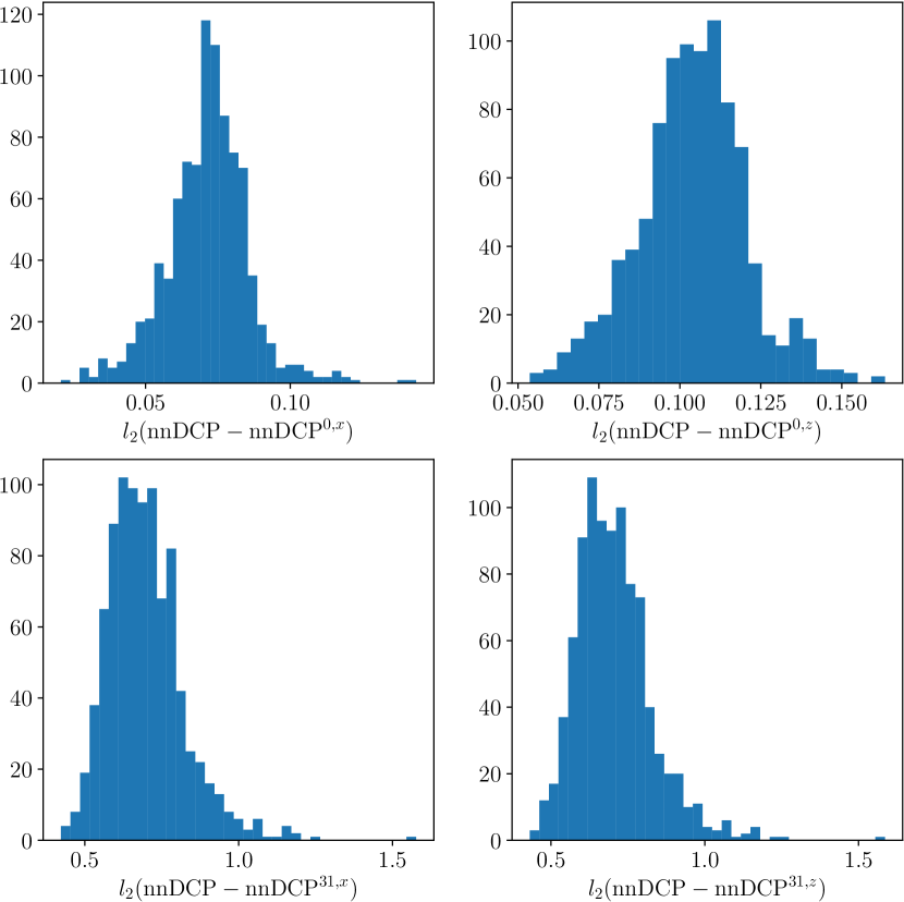
Figure 2: Exemplary histograms performing variation of ANN approximation. Histograms are generated from disturbances on set of 1000 NCP corresponding to random matrices, for fixed system $H_{\gamma}=\gamma\sigma_{y}\otimes{\rm 1l}.$

One can consider the median of the distribution of variations as the quantitative measure of the influence of the changes in the input signal on the resulting DCP. To check if medians of distributions of changes are similar, we perform Kruskal–Wallis statistical test for each pair of the changed coordinates (see Fig. 3(a)). Results presented in Fig 3(a) shows that most of the distributions received are statistically different regarding the median, i.e. most of the $p$–values is less than $0.05$. The values on the main diagonals, where we compared disturbances on the same controls in the same time slots, are equal to 1. This observation confirms that the test behaves appropriately in this case. On the other hand, one can observe that for time slots $10\leq i\leq 30$ Kruskal–Wallis test for distributions obtained for $NCP_{i+1,x}\pm\varepsilon$ and $NCP_{i,z}\pm\varepsilon$ gives $p$–values greater than $0.05$. Thus, the disturbances introduced in this time slots on $h_{x}$ and $h_{z}$ coordinates of $NCP$ results in similar variations of the resulting DCP. The situation is different for time slots $i\leq 10$, where one can see that the variation in DCP signal depends on which coordinate of the NCP signal is disturbed.

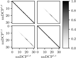
(a) $H_{\gamma}=\gamma\sigma_{y}\otimes{\rm 1l}$

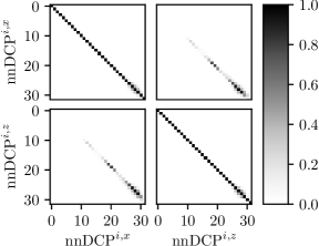
(b) $H_{\gamma}=\gamma{\rm 1l}\otimes\sigma_{y}$.

Figure 3: Plots of $p$–values of Kruskal–Wallis test for tested drift Hamiltonians. Each element $(l,k)$ of above matrix plots represents a $p$–value of the test between empirical distributions of changes implied by disturbances on $l$-th time slot and $k$-th time slot. The horizontal axis of the left column and the vertical axis of top row plots correspond to disturbances on $\sigma_{x}$ control, while horizontal axis of the right column and the vertical axis of the bottom plots correspond to disturbances on $\sigma_{x}$ control.

The similar effect can be observed if the drift Hamiltonian acts on the second qubit only. In this case we can consider experiment where the drift Hamiltonian is of the form

$$H_{\gamma}=\gamma{\rm 1l}\otimes\sigma_{y},$$ (13)

with $\varepsilon=0.1$ and $\gamma=0.2$.

The results of Kruskal–Wallis test for this situation are presented in Fig. 3(b). One can see that our approach suggests that there are similarities in distributions of variations implied by disturbances on different controls and near time slots. This suggests that local disturbances in control signals have a similar effect in the case of drift on the target system and drift on the auxiliary system.

Moreover, one can see that the constructed approximation exhibits symmetry of the model. This effect can be observed by analysing the disturbances of $h_{x}$ and $h_{z}$ controls in the same time slot. From the performed experiments one can see they give similar variations quantified by the distribution of DCP changes.

One should note that on plots in Fig. 3, where we compare variations of $\textrm{nnDCP}^{i,x}$ and $\textrm{nnDCP}^{i,z}$, $p$–values greater than $0.05$ are focused along the diagonal. This symmetry is not perfect, but one should note that training data are generated from random unitary matrices. Moreover, as we do not impose any restrictions on the training set to ensure the uniqueness of the correction scheme.

IV Discussions

In a case where Hamiltonian drift is absent $\gamma\neq 0$ and we want to find proper DCP for system with incoherent noise, things get more complicated. In our experiments we tested three kinds of Lindblad noise, namely

1. with one Lindblad operator $L=|0\rangle\langle 1|\otimes{\rm 1l}$,

2. with two Lindblad operators $L_{1}=\sigma_{z}\otimes{\rm 1l}$ and $L_{2}={\rm 1l}\otimes\sigma_{z}$,

3. and mixed two Lindblad operators $L_{1}=\sigma_{z}\otimes{\rm 1l}$ and $L_{2}=|0\rangle\langle 1|\otimes{\rm 1l}$.

For all this open system noise models, nnDCP obtains efficiency above 90% for $\gamma_{1}=\gamma_{2}\approx 0.01$. However, this strength of noise is so small that also NCP obtains similar efficiency. Therefore, the proposed model of the neural network does not correct NCP effectively, for incoherent types of noise.

Another important case in the context of quantum control is the robustness on the random fluctuations. In our experiments, we tried to generate nnDCP which will be robust for Gaussian fluctuations i.e.

$$\forall i\in\{0,\ldots,n-1\},\ j\in\{x,z\}\ nnDCP_{i,j}+\delta_{i,j},$$ (14)

where $\delta_{i,j}\sim\mathcal{N}(0,\sigma)$. The standard deviation we tested in two cases $\sigma=0.1$ and 0.2, while the model of Hmiltonian drift was $0.4(\sigma_{y}\otimes{\rm 1l})$.

During the training process, returned by ANN control pulses were copied ten times and to each copy we added Gaussian fluctuations. Such disturbed nnDCP were applied to cost function Eq. (8), and next the average fidelity was calculated. Unfortunately, after this training process artificial neural network doesn’t produce nnDCP which are more robust for random fluctuations. This failure might be caused by the fact that training of artificial neural network is based on gradient descent. As we know from Niu et al. (2018), gradient based algorithm does not give very good results. On the other hand, task with which we try to face is slightly different from the one in Niu et al. (2018), because we want to generalize correction scheme over all target unitaries.

V Concluding remarks

The primary objective of the presented work is to use artificial neural networks for the purpose of approximating the structure of quantum systems. We propose to use a bidirectional LSTM neural network. We argue that this type of artificial neural network is suitable to capture time-dependences present in quantum control pulses. We have developed a method of reconstructing the relation between control pulses in idealised case and control pulses required to implement quantum computation in the presence of undesirable dynamics. We argue that the proposed method can be a useful tool to study the manifold of quantum control pulses in the noisy regime, and to define new theoretical approaches to control noisy quantum systems.