Shape resonances of Be^- and Mg^- investigated with method of analytic continuation

Abstract

The regularized method of analytic continuation is used to study the low-energy negative ion states of beryllium (configuration 2$s^{2}\varepsilon p\;^{2}P$) and magnesium (configuration 3$s^{2}\varepsilon p\;^{2}P$) atoms. The method applies an additional perturbation potential and it requires only routine bound-state multi-electron quantum calculations. Such computations are accessible by most of the free or commercial quantum chemistry software available for atoms and molecules. The perturbation potential is implemented as a spherical Gaussian function with a fixed width. Stability of the analytic continuation technique with respect to the width and with respect to the input range of electron affinities is studied in detail. The computed resonance parameters $E_{r}$=0.282 eV, $\Gamma$=0.316 eV for the $2p$ state of Be^- and $E_{r}$=0.188 eV, $\Gamma$=0.167 for the $3p$ state of Mg^-, agree well with the best results obtained by much more elaborated and computationally demanding present-day methods.

I Introduction

Resonances in electron-atom or electron-molecule scattering, also addressed as transient negative ions, have attracted attention over the last decades. It is because these temporary states provide a pathway for electron-driven chemistry via dissociative electron attachment (DEA) and therefore, applications can be found in chemistry of the planetary atmospheres Carelli et al. (2013), nanolithography in microelectronic device fabrication van Dorp (2012); Thorman et al. (2015), and in cancer research where these states provide a mechanism for the DNA damage by low-energy electrons Pan et al. (2003); Zheng et al. (2006).

Accurate calculation of energies and lifetimes of the resonances represents a challenging task that is more complicated than the determination of energies of the bound atomic or molecular states. Temporary negative ions differ from the bound states in two important respects: (i) they are not stable and decay into various continua, (ii) corresponding poles of the $S$-matrix are complex and they are expressed by $E=E_{r}-i\Gamma/2$. There have been numerous studies published using several methods for determination of the resonance energies and widths. Stabilization methods Taylor and Hazi (1976); Hazi and Taylor (1970); Hazi et al. (1981); Frey and Simons (1986) search for a region of stability of the energies with respect to different confining parameters. Stieltjes imaging technique Hazi et al. (1981) allows to represent the resonant state by a square-integrable basis and the width is defined by the resonance-continuum coupling. Complex rotation methods Moiseyev (1998); McCurdy and Rescigno (1978); Reinhardt (1982) and the methods employing complex absorbing potential Riss and Meyer (1993); Feuerbacher et al. (2003) compute complex resonant energy as an eigenvalue of a complex, non-Hermitian Hamiltonian.

Recently the method of analytic continuation in coupling constant (ACCC) Kukulin and Krasnopolsky (1977); Krasnopolsky and Kukulin (1978); Kukulin et al. (1988) has been applied to several molecular targets, such as N₂ Horáček et al. (2010); White et al. (2017), ethylene Horáček et al. (2014); Sommerfeld et al. (2017), and amino acids Papp et al. (2013). Furthermore, the known low-energy analytic structure of the resonance was incorporated into the inverse ACCC (IACCC) method providing so-called regularized analytic continuation (RAC) method. The RAC method was successfully employed for determination of $\pi^{*}$ resonances of acetylene Čurík et al. (2016) and diacetylene Horáček et al. (2015) anions, proving that the ACCC method can yield accurate resonance energies and widths for various molecular systems using data obtained with standard quantum chemistry codes.

Common feature of all methods of analytic continuation is an application of the perturbation potential $\lambda V$ to the multi-electron Hamiltonian $H$, i.e. $H\rightarrow H+\lambda V$. The role of this attractive perturbation is to transform the resonant state into a bound state. Although the RAC method was developed for strictly short-range perturbation $V$, authors were able to successfully use the Coulomb potential in its stead Čurík et al. (2016); Horáček et al. (2015). This obvious inconsistency can yield reasonable results, because in practical applications the perturbation potential is often projected on a finite set of short-range basis functions, e.g. Gaussian functions used by the quantum chemistry software. However, so obtained weakly-bound states need to be examined carefully because they may, in fact, be Rydberg states supported by the basis and the long-range tail of the Coulomb perturbation $V$ Horáček et al. (2015). Such states need to be excluded from the continuation procedure as they do not represent a resonance transferred to a bound state. In order to avoid such complications, in the present study we adopt a short-range perturbation potential in a form the Gaussian function

$$V(r)=-\lambda e^{-\alpha r^{2}}\;.$$ (1)

This choice of the perturbation was recently evaluated by White et al. White et al. (2017) and applied to the well-known ${}^{2}\Pi_{g}$ resonance of N${}_{2}^{-}$. Furthermore, Sommerfeld and Ehara Sommerfeld and Ehara (2015) introduced another short-range potential, termed as Voronoi soft-core potential, which they successfully used to analyze the ${}^{2}\Pi_{u}$ resonance of CO${}_{2}^{-}$.

Present analysis of the Gaussian perturbation potential (1) will be carried out for expectedly simpler problems - atomic shape resonances of beryllium and magnesium. Both atoms are known to possess a $p$-wave shape resonance very close to the elastic threshold. While in the case of the Mg^- the agreement between the available computed resonance parameters Hunt and Moiseiwitsch (1970); Krylstedt et al. (1987); Kim and Greene (1989) and the experimental data Burrow et al. (1976); Buckman and Clark (1994) is quite good, the situation is very different for the beryllium atom. There has been a great number of theoretical studies Kurtz and Öhrn (1979); Kurtz and Jordan (1981); McCurdy et al. (1980); Rescigno et al. (1978); McNutt and McCurdy (1983); Krylstedt et al. (1988); Zhou and Ernzerhof (2012); Venkatnathan et al. (2000); Samanta and Yeager (2008, 2010); Tsednee et al. (2015); Zatsarinny et al. (2016) aiming to numerically characterize Be^- 2$s^{2}\varepsilon p\;^{2}P$ resonance, with various levels of success. Table III in Ref. Tsednee et al. (2015) clearly summarizes that the theory of the last four decades predicts the resonance position between 0.1 and 1.2 eV and the resonance width between 0.1 and 1.7 eV. Even the most recent calculations differ by about a factor of 3 for the two resonant parameters. Moreover, there are no experimental data available for the Be^- resonance that could narrow the spread of all the available theoretical predictions.

Convergence patters shown in Refs. Tsednee et al. (2015); Zatsarinny et al. (2016) demonstrate that the Be^- resonance may be very sensitive to an accurate description of the electronic correlation energy. Therefore, in the present study we employ coupled-clusters (CCSD-T) and full configuration interaction (FCI) methods for the perturbed Be^- electron affinities that will be then continued the complex plane by the RAC method. The basic ideas of the RAC method are given in the Sec. II. Quick summary of the quantum chemistry details is presented in Sec. III. In Sec. IV we analyze the stability and accuracy of the RAC method with the Gaussian perturbation potential (1). Then conclusions follow.

II RAC method

The RAC method represents a very simple method for calculation of resonance energies and widths which embraces all known analytical features of coupling constant $\lambda(\kappa)$ near the zero energy Horáček et al. (2015). The method works as follows:

• The atom or molecule is perturbed by an attractive interaction $V$ multiplied by a real constant $\lambda$

  $$\rm H_{neutral}\rightarrow H_{neutral}+\lambda V\;,$$ (2)

  and bound states energies $E^{N}_{i}$ of the neutral state are calculated for a set of values $\lambda_{i}$.

• The same procedure is carried out for the corresponding negative ion

  $$\rm H_{ion}\rightarrow H_{ion}+\lambda V\;,$$ (3)

  where the bound state energies $E^{I}_{i}$ are calculated for the same values of $\lambda_{i}$.

• Both energies are subtracted forming the electron affinity in the presence of the perturbation potential $V$

  $$E^{N}_{i}-E^{I}_{i}=E_{i}=\kappa_{i}^{2}\;.$$ (4)

The new set of data points $\{\kappa_{i},\lambda_{i}\}$ is then used to fit the function

$$\lambda(\kappa)=\lambda_{0}\frac{(\kappa^{2}+2\alpha^{2}\kappa+\alpha^{4}+\beta^{2})(1+\delta^{2}\kappa)}{\alpha^{4}+\beta^{2}+\kappa(2\alpha^{2}+\delta^{2}(\alpha^{4}+\beta^{2}))}.$$ (5)

It is represented as a Padé 3/1 function and it defines the level of complexity of the pole behavior at the low bound or continuum energies. We term it as RAC [3/1] method. The origin of its form and the fit formulae for [2/1], [3/2], and [4/2] methods can be found in Ref. Čurík et al. (2016). The parameters of the [3/1] fit, namely $\alpha,\beta,\delta$ and $\lambda_{0}$ are found by minimizing the $\chi^{2}$ functional

$$\chi^{2}=\frac{1}{N}\sum_{i=1}^{N}\frac{1}{\varepsilon_{i}^{2}}\left|\lambda(\kappa_{i})-\lambda_{i}\right|^{2},$$ (6)

where $N$ denotes the number of the points used, while $\kappa_{i}$ and $\lambda_{i}$ are the input data. Once an accurate fit is found, only the parameters $\alpha$ and $\beta$ determine the resonance energy

$$E_{r}=\beta^{2}-\alpha^{4}\;,$$ (7)

and the resonance width

$$\Gamma=4\beta\alpha^{2}\;.$$ (8)

Role of the parameter $\delta$ is to describe a virtual state with $E_{v}=-1/\delta^{4}$. Even in the case the studied system does not possess a virtual state this parameter represents a cumulative effect of the other resonances and other poles not explicitly included in the model. The weights $\varepsilon_{i}$ (accuracy of the data) in Eq. (6) are generally unknown. The calculation can be routinely performed with constant $\varepsilon_{i}$ = 1 or, if an importance of the data points closest to the origin needs to be stressed, increasing weights sequence (e.g. $\varepsilon_{i}$ = i) can be used.

The RAC method has been recently critically evaluated by White et al. White et al. (2017). Authors tested three types of the perturbation potential

$$V(r) = -\frac{\lambda}{r},$$ (9)

$$V(r) = -\lambda\frac{e^{-\alpha r^{2}}}{r},$$ (10)

$$V(r) = -\lambda e^{-\alpha r^{2}}\;,$$ (11)

and they suggested that the attenuated Coulomb potential (10) is the best choice out of the three options and the Gaussian potential (11) does not represent a good choice for the RAC method. All these potentials are easily implemented into the standard quantum chemistry codes. The aim of the present contribution is twofold:

• to explore application of the Gaussian-type perturbation and to find its parameters that allow accurate extraction of the resonance data with the RAC method

• to demonstrate that the RAC method can be applied with success to low-lying atomic shape resonances

Before applying the RAC method one must consider two important issues.

• First is a choice of the perturbation potential, i.e. in the present context the choice of the exponent $\alpha$ in Eq. (11). Presently there exist no general rule, no guide that helps us to choose the perturbation potential. Therefore, it is necessary to perform calculations for a set of values of the parameter $\alpha$ to find an optimal choice. If the optimal range of values is found, it is reasonable to expect that the obtained resonance data should stabilize in such a range, because the exact function $\lambda(\kappa)$ gives the same resonant data for every choice of the perturbation potential. Since the present [3/1] RAC function is only approximative, one can only expect an existence of a plateau that gives approximative values of the resonance parameters.

• The RAC method represents essentially a low-energy approximation to the exact function $\lambda(\kappa)$. It is therefore obvious that the method should be used in a range of energies (or momenta) limited by some maximal energy $E_{M}$. Our empirical experience shows that $E_{m}\sim 8E_{r}$ ($E_{r}$ is the sought resonance energy) gives a reasonable estimate for the range of energies.

III Electron affinities

Ab initio calculations for the electron affinities $E_{i}(\lambda_{i})$ in presence of the external Gaussian field (11) were carried out using the CCSD-T Knowles et al. (1993); Deegan and Knowles (1994) and FCI methods as implemented in MOLPRO 10 package of quantum-chemistry programs Werner et al. (2010). Core of the basis set employs Dunning’s augmented correlation-consistent basis of quadruple-zeta quality aug-cc-pVQZ Prascher et al. (2011) for both atoms, Be and Mg. This basis set was additionally extended, in an even-tempered fashion, by 2 ($s$, $d$, $f$, $g$)-type functions and 6 $p$-type functions.

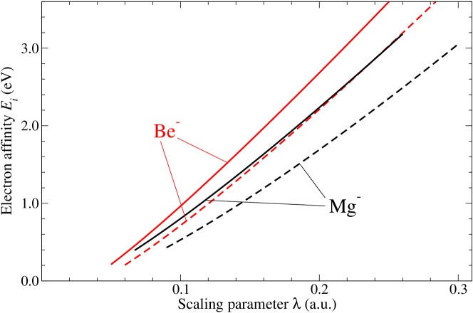
Figure 1: (Color online) Electron affinities of Be^- and Mg^- ions under the influence of the perturbation potential (11). Full lines are shown for the exponent $\alpha$ = 0.025, while the broken lines are for $\alpha$ = 0.035. Red color (light gray) describes the Be^- ion and the black color is for the Mg^-.

Calculations for the neutral atoms and corresponding negative ions used the same basis sets and the same correlation methods (CCSD-T or FCI). Typical dependence of the electron affinities on external field (11) is shown in Fig. 1 for both negative ions, Be^- and Mg^-, and in the range of energies used for the present analytic continuation. Fig. 1 yields the following observations:

• As expected, the weaker perturbation potential with $\alpha$ = 0.035 requires a stronger scaling parameter $\lambda$ to achieve the same binding negative ion energies as the perturbation with $\alpha$ = 0.025.

• Surprisingly, a larger scaling parameter (stronger perturbation) is necessary to bind the Mg^- resonance that lies closer to the zero when compared to the Be^- resonance (as will be seen below). Such behavior may be caused by the spatial extent of the Mg^- 3$p$ resonant wave function when compared to the reach of the 2$p$ wave function of the Be^- ion.

• The lowest binding energies are not included in the continuation input data because of the difficulties we encountered while using the quantum chemistry software. Hartree-Fock method is known to destabilize in very diffused basis sets, however low binding energies are inaccurate if a more compact basis is used.

Most of the present results were obtained with the CCSD-T method. However, once the the optimal exponent $\alpha$ (see the Sec. IV) was found for the beryllium atom, the affinity curve shown in Fig. 1 was also recomputed with the expensive FCI method and the basis as described above.

IV Results

As discussed in Sec. II, our goal is to search for regions of stable results with respect to the two optimization parameters. First is the range of the input electron affinities defined by maximal affinity $E_{M}$. The second parameter, the exponent $\alpha$ in Eq. (11) defines the shape of the perturbation potential.

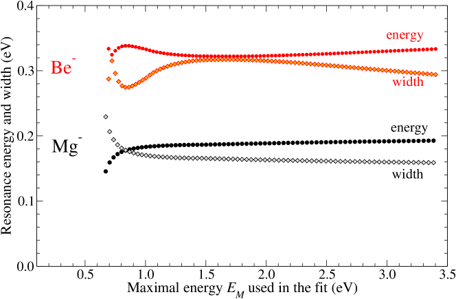
Figure 2: (Color online) Resonance energy (shown as circles) and width (displayed as diamonds) calculated for Be^- and Mg^- as functions of the energy extent defined by the maximal energy $E_{M}$. The exponents $\alpha$ are fixed at $\alpha$ = 0.035 for Be^- and $\alpha$ = 0.025 for Mg^-.

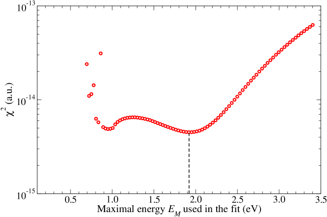
Figure 3: (Color online) Quality of the RAC fit for the resonance of Be^- as a function of the maximal energy. Exponent $\alpha$ is fixed at 0.035 and the increasing weights set $\varepsilon$ = $i$ are used.

Typical dependence of the resonance parameters on the maximal energy is shown in Fig. 2 for the fixed $\alpha$ parameters. It is clear that the stability is little worse for the Be^- ion when compared to Mg^- ion. However, it is possible to narrow the spread of the obtained resonance data by considering the value of $\chi^{2}$ defined by Eq. (6). Fig. 3 shows the dependence of $\chi^{2}$ quantity on the maximal energy $E_{M}$. A pronounced minimum at $E_{M}$ = 1.92 eV is clearly visible. This allows an application of a condition of the best fit. Such a restriction leads to a well defined $E_{M}$ for each choice of the perturbation parameter $\alpha$ producing a data sets shown in Fig 4.

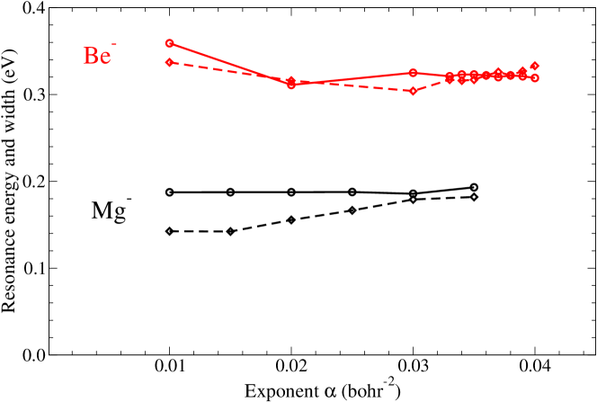
Figure 4: (Color online) Resonance energy $E_{r}$ (circles connected full lines) and the resonance width $\Gamma$ (diamonds connected with dashed lines) as functions of $\alpha$ parameter of the perturbation potential.

For beryllium the resonance position and width stabilizes for $\alpha>$ 0.02. The best fit is obtained for $\alpha$ = 0.035 resulting in $E_{r}$ = 0.323 eV and $\Gamma$ = 0.317 eV. In order to estimate accuracy of the correlation energy provided by the CCSD-T method we also recomputed this final results with the FCI method. The FCI affinities yield $E_{r}$ = 0.282 eV and $\Gamma$ = 0.316 eV. Detailed summary of the available theoretical results for the Be^- resonance was presented in Tab. III of Ref. Tsednee et al. (2015). A comparison with the most recent computations will be given in Sec. V.

In case of magnesium ion the resonance energy is very stable over the whole range of examined perturbation parameters $\alpha$. However, the width exhibits a weak dependence on the exponent $\alpha$. This feature may indicate that the low-order RAC method is inadequate for the Mg^- resonance. Nonetheless, the best fit is obtained for $\alpha$ = 0.025, giving $E_{r}$ = 0.188 eV and $\Gamma$ = 0.167 eV. The available data for the Mg^- resonance are summarized in Tab. 1.

Table 1: Comparison of the available data for the resonance energy $E_{r}$ and the resonance width $\Gamma$ for the 3s${}^{2}\varepsilon$p ²P state of atomic magnesium.

Method	Resonance energy $E_{r}$(eV)	Resonance width $\Gamma$(eV)
Model potential Hunt and Moiseiwitsch (1970)	0.37	0.10
Model potential Kim and Greene (1989)	0.161	0.160
Complex rotation Krylstedt et al. (1987)	0.08	0.17
Stabilization Chao et al. (1990)	0.14	0.08
Complex SCF McCurdy et al. (1981)	0.50	0.54
Finite elements Gallup (2011)	0.159	0.12
Experiment Burrow et al. (1976)	0.15$\pm$0.03	$\sim$0.14
Recommended value Buckman and Clark (1994)	0.15	0.16
Present RAC	0.19	0.16

Presently computed resonance energy is about 40 meV higher that the experimental value of Burrow et al. Burrow and Comer (1975); Burrow et al. (1976). Such a discrepancy may have several possible reasons:

• The experimental resolution is about 30–40 meV Burrow et al. (1976).

• Discrepancy between the correlation energies of the CCSD-T and FCI methods and the present basis set is about 41 meV for the electron affinity of the beryllium atom. Similar difference can also be expected for the magnesium. Moreover, weaker stability of $\Gamma$ with respect to the perturbation potential (shown in Fig. 4) indicates that higher order continuation may be necessary.

• The experimental resonance energy Burrow et al. (1976) was determined from the maximum of the measured cross section, whereas present method defines the resonance energy from a pole of the $S$-matrix. The two definitions give similar results for a narrow resonance ($\Gamma<E_{r}$), but for for a broader resonance ($\Gamma\geq E_{r}$), as in the present case, the results may differ.

V Conclusions

Present study confirms the observations of White et al. White et al. (2017) in which the authors state that the Gaussian perturbation potential is more difficult to apply than potentials possessing the Coulomb singularity. It has been shown in the case of a model potential White et al. (2017) that the trajectory of the resonant pole is more complicated for the Gaussian perturbation. In the present study we have shown that in order to obtain stable results, the RAC method must be restricted to fairly low electron affinities and a careful analysis of the results with respect to the width of the perturbation potential must be carried out.

Such procedure allowed us to apply the RAC method to one of the remaining enigmas among shape resonances of small atoms, the 2$s^{2}\varepsilon p\;^{2}P$ resonance of Be^-. To the best of our knowledge there are no experimental data available for this resonance. Important role of the correlation energy in this system creates a challenging task for the theory, albeit the fact that Be^- possess only 5 electrons. Consequently, about two dozens of theoretical predictions (found in Ref. Kurtz and Öhrn (1979); Kurtz and Jordan (1981); McCurdy et al. (1980); Rescigno et al. (1978); McNutt and McCurdy (1983); Krylstedt et al. (1988); Zhou and Ernzerhof (2012); Venkatnathan et al. (2000); Samanta and Yeager (2008, 2010); Tsednee et al. (2015); Zatsarinny et al. (2016)) do not result in any kind of a consensus. Two methods with high level of correlation description, the CCSD-T and FCI methods, were applied in the present study. While the position of the resonance shifts to the lower energies by about 41 meV for the more accurate FCI method, the resonance width was found insensitive to the correlation treatment. Presently calculated FCI resonant energy $E_{r}$ = 0.282 eV and width $\Gamma$ = 0.316 eV are in a good agreement with the complex CI results of McNutt and McCurdy McNutt and McCurdy (1983) that predict the $E_{r}$ = 0.323 eV and $\Gamma$ = 0.296 eV. Recent scattering calculations Zatsarinny et al. (2016) determined the resonance with $E_{r}$ = $0.31\pm 0.04$ eV and $\Gamma$ = $0.40\pm 0.06$ eV again in a good agreement with the present results. However, another set of recent calculations by Tsednee et al. Tsednee et al. (2015) place the resonance at $E_{r}$ = 0.756 eV and $\Gamma$ = 0.874 eV.

In case of the 2$s^{2}\varepsilon p\;^{2}P$ resonance of Mg^- a comparison with the experiment is available. Although, the present calculations determine the resonance about 40 meV higher than the experiment Burrow et al. (1976), they still exhibit the best agreement with the experimental data among the ab-initio methods.