Intermittent electron density and temperature fluctuations and associated fluxes in the Alcator C-Mod scrape-off layer

Abstract

The Alcator C-Mod mirror Langmuir probe system has been used to sample data time series of fluctuating plasma parameters in the outboard mid-plane far scrape-off layer. We present a statistical analysis of one second long time series of electron density, temperature, radial electric drift velocity and the corresponding particle and electron heat fluxes. These are sampled during stationary plasma conditions in an ohmically heated, lower single null diverted discharge. The electron density and temperature are strongly correlated and feature fluctuation statistics similar to the ion saturation current. Both electron density and temperature time series are dominated by intermittent, large-amplitude burst with an exponential distribution of both burst amplitudes and waiting times between them. The characteristic time scale of the large-amplitude bursts is approximately $15\,\mu\mathrm{s}$. Large-amplitude velocity fluctuations feature a slightly faster characteristic time scale and appear at a faster rate than electron density and temperature fluctuations. Describing these time series as a superposition of uncorrelated exponential pulses, we find that probability distribution functions, power spectral densities as well as auto-correlation functions of the data time series agree well with predictions from the stochastic model. The electron particle and heat fluxes present large-amplitude fluctuations. For this low-density plasma, the radial electron heat flux is dominated by convection, that is, correlations of fluctuations in the electron density and radial velocity. Hot and dense blobs contribute approximately $6\%$ of the total fluctuation driven heat flux.

I Introduction

Turbulent flows in the scrape-off layer (SOL) of magnetically confined plasmas have received great attention recently. Experimental analyses have demonstrated that plasma blobs propagating through the scrape-off layer towards the vessel wall dominate the plasma particle and heat fluxes at the outboard mid-plane LABEL:labombard-2001,_rudakov-2002,_boedo-2003,_rudakov-2005,_garcia-2007-nf,_garcia-2007-nf,_garcia-2008-ppcf,_fedorczak-2009,_carralero-2014,_graves-2005,_antar-2001,_walkden-2017. In order to assess expected erosion and damage to the plasma enclosing vessel, the statistics of the impinging plasma fluxes are of great interest LABEL:federici-2001,_loarte-2007_nf,_lipschultz-2007,_wenninger-2017.

Plasma blobs are pressure perturbations spatially localized in the plane perpendicular to the magnetic field and elongated along the magnetic field lines. They are believed to be created in the vicinity of the last closed magnetic flux surface with particle density perturbation amplitudes comparable in magnitude to the average scrape-off layer particle density. At the outboard mid-plane location the magnetic curvature vector and field strength gradient point towards the magnetic axis. This causes an electric polarization of the blob structure due to magnetic curvature and gradient drifts. The resulting electric field propagates the blob towards the vessel wall, resulting in large cross-field particle and heat fluxes onto plasma facing components. LABEL:krash-2001,_dippolito-2002,_bian-2003,_yu-2003,_myra-2004,_aydemir-2005,_garcia-2006.

Scrape-off layer plasma fluctuations furthermore exhibit several universal features. Time series data of plasma density fluctuations feature non-gaussian values of sample skewness and flatness and their probability density functions (PDFs) present elevated tails for large amplitude events. This feature has been observed in experiments LABEL:antar-2001,_antar-2003,_graves-2005,_xu-2005,_garcia-2013,_kube-2016-ppcf,_theodorsen-2016-php,_theodorsen-2017-nf,_garcia-2016-nme,_walkden-2017 as well as in numerical simulations LABEL:ghendrih-2003,_garcia-2004,_bisai-2005,_garcia-2008-ppcf,_militello-2012 and is well documented to be due to the radial propagation of plasma blobs LABEL:terry-2003,_zweben-2004,_terry-2005,_zweben-2006,_agostini-2011,_maqueda-2011,_garcia-2013,_kube-2013. A quadratic relation between sample skewness and flatness has been reported from several experiments LABEL:labit-2007,_sattin-2009,_banerjee-2012,_garcia-2013-jnm,_banerjee-2014,_kube-2016-ppcf,_theodorsen-2016-ppcf,_garcia-2016. Conditionally averaged waveforms of electron density time series exhibit approximately two-sided exponential waveform shapes LABEL:boedo-2003,_rudakov-2005,_garcia-2007-nf,_silva-2009,_garcia-2013,_tanaka-2015,_theodorsen-2016-ppcf,_garcia-2016,_kube-2016-ppcf. Several experiments report large-amplitude electron density fluctuations in phase with an outwards $\bm{E}\times\bm{B}$ drift velocity, that is radial particle flux events LABEL:boedo-2003,_grulke-2006,_saha-2008,_silva-2009,_kube-2016-ppcf,_theodorsen-2016-ppcf.

A recently developed stochastic model describes such time series as a super-position of uncorrelated pulses LABEL:garcia-2012. Assuming an exponential pulse shape and exponentially distributed pulse amplitudes and waiting times between pulses LABEL:garcia-2013,_garcia-2013-jnm,_garcia-2015,_theodorsen-2016-php,_garcia-2016-nme it predicts the fluctuation amplitudes to be Gamma distributed. The quadratic relation between moments of skewness and flatness of a Gamma distributed variable is in excellent agreement with the quadratic relation observed in experiments. This model furthermore predicts the experimentally observed exponential density profiles in scrape-off layer plasmas LABEL:garcia-2016,_militello-2016. The stochastic model has been generalized to describe general pulse shapes as well as additive noise. Analytic expressions of probability density functions, auto-correlation functions, power spectral densities and level crossing rates have been derived LABEL:theodorsen-2016-php,_garcia-2016,_theodorsen-2017-ps,_garcia-2017-ac. In this contribution it is demonstrated that the model predictions compare favorably with measurements of the fluctuating electron density and temperature, as well as with the radial velocity. It should be noted that by constructing the stochastic model as a superposition of individual pulses, the underlying non-linear dynamics of the plasma is parameterized. Specifically, the steepening of radially propagating blob structures is modeled by exponential pulse shapes. Another approach, which proposes a stochastic differential equations to describe the non-linear plasma dynamics, under the constraint that the fluctuations are Gamma distributed, has recently been explored LABEL:mekkaoui-2013.

Scrape-off layer plasmas are usually diagnosed with Langmuir probes. They allow for three fundamental modes of operation. One way is to apply a sweeping voltage to a Langmuir electrode. This allows the plasma density, the electric potential as well as the electron temperature to be inferred on the time scale of the sweeping voltage. This time scale is commonly of the orders of milliseconds, as to avoid hysteresis effects which arise at higher sweeping frequencies LABEL:muller-2010. On the other hand, the time scale associated with blob propagation is on the order of microseconds. Conventional sweeping modes can thus not be used to investigate plasma fluctuations.

A second way is to bias the Langmuir electrode to a large negative electric potential relative to the vacuum vessel. This way the electrode draws the ion saturation current LABEL:hutchinson-book

$$I_{\mathrm{s}} =\frac{1}{2}en_{\mathrm{e}}A_{\mathrm{p}}\sqrt{\frac{k_{\mathrm{b}}T_{\mathrm{e}}}{m_{\mathrm{i}}}}.$$ (1)

Here $e$ is the elementary charge, $n_{\mathrm{e}}$ is the electron density, $T_{\mathrm{e}}$ is the electron temperature, $m_{\mathrm{i}}$ is the ion mass and $A_{\mathrm{p}}$ is the current collecting probe area. This assumes that the ion temperature is zero, although it is typically larger than the electron temperature for the measurements in this paper. Employing a Reynolds decomposition of the time-dependent quantities in Eq. ( 1), as $u(t)=u_{0}+\widetilde{u}(t)$ for a variable u, shows that fluctuations in $n_{\mathrm{e}}$ and $T_{\mathrm{e}}$ perturb the ion saturation current as

$$\frac{\widetilde{I}_{\mathrm{s}}}{I_{\mathrm{s},0}}\approx\left(\frac{\widetilde{n}_{\mathrm{e}}}{n_{\mathrm{e},0}}+\frac{1}{2}\frac{\widetilde{T}_{\mathrm{e}}}{T_{\mathrm{e},0}}\right).$$ (2)

Here the factor $1/2$ comes from an expansion of the square-root for small relative electron temperature fluctuations. For equal relative fluctuations of the electron density and temperature the electron density contributes twice as much to the relative fluctuation of the ion saturation current than the electron temperature fluctuation. With no fast measurements of $T_{\mathrm{e}}$ at hand, a constant value is often assumed for $T_{\mathrm{e}}$ in Eq. ( 1) to find $n_{\mathrm{e}}$ given $I_{\mathrm{s}}$.

A third mode of operation is to electrically isolate the Langmuir electrode. In this mode, it assumes the floating potential

$$V_{\mathrm{f}} =V_{\mathrm{p}}-\Lambda T_{\mathrm{e}},$$ (3)

where $V_{\mathrm{p}}$ is the plasma potential and $\Lambda\approx 2-3$ in scrape-off layer plasmas LABEL:stangeby-book,_rohde-1996. Using again a Reynolds decomposition, the fluctuating floating potential is given by $\widetilde{V}_{\mathrm{f}}=\widetilde{V}_{\mathrm{p}}-\Lambda\widetilde{T}_{\mathrm{e}}$. Thus, perturbations in the floating potential are equally due to fluctuations in the plasma potential and the electron temperature. Fast measurements of $T_{\mathrm{e}}$ in the scrape-off layer are often unavailable such that $n_{\mathrm{e}}$ is approximated by $I_{\mathrm{s}}$ and the plasma potential is estimated by the floating potential. From this, an estimate of the radial $\bm{E}\times\bm{B}$ drift velocity can be calculated given two spatially separated measurements of the floating potential. It was recently observed that perturbations of the electron temperature may alter the estimated radial drift velocity LABEL:horacek-2010,_nold-2012,_gennrich-2012.

Since plasma blobs present perturbations of the plasma density, temperature and electric potential, real time measurements of all three quantities from a single point are desirable as to precisely quantify their contributions to cross-field transport in the scrape-off layer. Recent probe designs, such as ball pen probes LABEL:adamek-2004,_adamek-2009 and emissive probes LABEL:schrittwieser-2002,_schrittwieser-2008,_ionita-2011,_adamek-2014 allow fast sampling of the plasma potential but to evaluate the electron temperature one still needs to combine data from multiple electrodes.

Langmuir probe implementations that utilize multiple electrodes to provide real time samples of the fluctuating plasma parameters, such as triple probes, are routinely operated in several major tokamaks LABEL:lin-1992,_asakura-1995,_yang-2003,_kim-2016. In this configuration current and voltage samples from different Langmuir electrodes are combined as to estimate the fluctuating electron density, the plasma potential, and the electron temperature in real time. On the other hand the equations of the triple probe configuration assume that the electrodes sample a homogeneous plasma. These assumptions are often violated in the scrape-off layer, where the characteristic length of the turbulence structures may be smaller than the separation of the Langmuir electrodes. Triple probe configurations have also been implemented in the time domain, removing the assumption of a homogeneous plasma LABEL:meier-1995,_meier-1997,_meier-2001. This configuration requires two spatially separated Langmuir electrodes. Periodically biasing the electrodes to three different bias voltages allows to infer the electron density and temperature, as well as the plasma potential at each Langmuir electrode independently.

Fast measurements of electron temperature fluctuation in scrape-off layer plasmas are sparse. Measurements based on the method of harmonics LABEL:boedo-1999 taken in the DIII-D tokamak suggest that fluctuations of the electron temperature and the electric drift velocity appear on average in phase with fluctuations in the electron density LABEL:rudakov-2002,_rudakov-2005. However, the method of harmonics has a time resolution of $10\,\mu\mathrm{s}$, comparable to the time scale of the turbulence structures in the plasma LABEL:boedo-1999. Analysis of an $8\,\mathrm{ms}$ long electron temperature data time series, taken by a triple probe configuration in the SINP tokamak, suggests that it presents the same non-gaussian features as commonly observed in electron density time series: the frequent arrival of large-amplitude bursts and heavy-tailed histograms LABEL:saha-2008. Recent measurements reported from ASDEX Upgrade confirm that fluctuations of the electron density and temperature appear in phase, together with fluctuations in the plasma potential LABEL:horacek-2010. It was furthermore reported that the temperature fluctuations show on average a temporal asymmetry around the density peaks. Relative fluctuation levels of the electron temperature were found to be lower by a factor of approximately $2-3$ than for the electron density.

The novel mirror Langmuir Probe (MLP) biasing technique allows for fast sampling of the ion saturation current, the electron temperature and the floating potential at a single sampling position LABEL:labombard-2007,_labombard-2014. This diagnostics consists of three major components. The actual mirror Langmuir probe is an electronic circuit that generates a current-voltage (I-V) characteristic with the three adjustable parameters $I_{\mathrm{s}}$, $T_{\mathrm{e}}$, and $V_{\mathrm{f}}$:

$$I_{\mathrm{MLP}} =I_{\mathrm{s}}\left[\exp\left(\frac{V-V_{\mathrm{f}}}{T_{\mathrm{e}}}\right)-1\right]$$ (4)

The second main component is a Langmuir electrode immersed in the plasma to be sampled. Both components are connected to a fast switching biasing waveform. The bias waveform switches between the states $(V^{+},V^{0},V^{-})$, such that the Langmuir electrode draws approximately $\pm I_{\mathrm{s}}$ at the states $V^{\mp}$ and zero net current when biased to $V^{0}$, as shown in Fig. 1 of LABEL:labombard-2014. Every $300\,\mathrm{ns}$ the bias voltage state is updated. Current samples from the MLP and the Langmuir electrode are compared after the bias voltage has settled. In order to minimize the deviation between the two sample pairs, the MLP adjusts the $I_{\mathrm{s}}$, $T_{\mathrm{e}}$, and $V_{\mathrm{f}}$ parameters dynamically. The main task of the MLP circuit is to set and maintain the optimal range of the bias voltages such that a complete I-V characteristic can be reconstructed from measurements at the Langmuir electrode at the three bias voltages states. Samples of the I-V response from the MLP and the Langmuir electrode are digitized at $3\,\mathrm{MHz}$, synchronized to the states $V^{+}$, $V^{0}$, and $V^{-}$. The current and voltage samples of the Langmuir electrode are then used for a fit to the I-V characteristic as to obtain $T_{\mathrm{e}}$, $V_{\mathrm{f}}$ and $I_{\mathrm{s}}$. The time staggering of the three sequential measurements voltages is neglected. Time series of the fit parameters at a sampling frequency of $1\,\mathrm{MHz}$ are obtained by mapping them one-to-one to the time samples of the voltage states $V^{+}$, $V^{0}$ and $V^{-}$. Finally, the data time series of the $T_{\mathrm{e}}$, $V_{\mathrm{f}}$, and $I_{\mathrm{s}}$ fit parameters are linearly interpolated on the same time base with $3\,\mathrm{MHz}$ sampling frequency. From these sample values the electron density and the plasma potential are calculated LABEL:labombard-2014.

This contribution presents a statistical analysis of exceptionally long data time series measured by the MLP in stationary plasma conditions. Section II describes the experimental setup and Sec. III describes the data analysis methods employed. The statistical properties of the ion saturation current, floating potential, as well as electron density and temperature are discussed in Sec. IV. Fluctuation time series of the radial velocity, the radial electron particle and heat fluxes are analyzed in Sec. V. A discussion and a conclusion of the results are given in Secs. VI and VII. Supplementary information on the stochastic model and on analysis of the MLP data is given in the Appendices A and B.

II Experimental setup

Alcator C-Mod is a compact, high-field tokamak with major radius $R=0.68\,\mathrm{m}$ and minor radius $a=0.21\,\mathrm{m}$ LABEL:hutchinson-1994,_greenwald-2013,_greenwald-2014. It allows for an on-axis magnetic field strength of up to $8\,\mathrm{T}$ so as to confine plasmas with up to two atmospheres pressure. In this contribution we investigate the outboard mid-plane scrape-off layer of an ohmically heated plasma in a lower single-null diverted magnetic configuration with an on-axis toroidal field of $B_{\mathrm{T}}=5.4\,\mathrm{T}$. The toroidal plasma current for the investigated discharge is $I_{\mathrm{p}}=0.55\,\mathrm{MA}$ and the line averaged core plasma density is given by $\overline{n}_{\mathrm{e}}/n_{\mathrm{G}}=0.12$, where $n_{\mathrm{G}}$ is the Greenwald density. Such low density plasmas feature a far scrape-off layer with vanishing electron pressure gradients along magnetic field lines. The temperature drop from outboard mid-plane to the divertor plates is supported by the divertor sheaths LABEL:lipschultz-2007-fst.

A Mach probe head was dwelled at the limiter radius, approximately $0.11\,\mathrm{m}$ above the outboard mid-plane location. Its four electrodes are arranged in a pyramidal dome geometry on the probe head such that they sample approximately the same magnetic flux surface. Each electrode is connected to a MLP bias drive, and labeled northeast, southeast, southwest and northwest. Tracing a magnetic field line from the outboard mid-plane to the probe head, the east electrodes are in the shadow of the west electrodes, with the south electrodes facing the outboard mid-plane. The MLPs obtain $I_{\mathrm{s}}$, $V_{\mathrm{f}}$, and $T_{\mathrm{e}}$ from fits to the I-V samples with a sampling rate of approximately $1\,\mathrm{MHz}$. Further details on the probe head are given in LABEL:smick-2009.

III Data analysis

MLPs have been used successfully to measure profiles of average values and relative fluctuation levels LABEL:labombard-2014. However, large-amplitude fluctuations in the far scrape-off layer present challenges to interpreting the reported fit values $I_{\mathrm{s}}$, $V_{\mathrm{f}}$, and $T_{\mathrm{e}}$. The MLP dynamically updates the voltage states $V^{+}$ and $V^{-}$ relative to a running average of electron temperature samples over a  $2\,\mathrm{ms}$ window, $V^{+}-V^{-}<4\,\overline{T}_{\mathrm{e}}$ holds, where $\overline{T}_{\mathrm{e}}$ denotes this running average. When the instantaneous electron temperature at the Langmuir electrode significantly exceeds $\overline{T}_{\mathrm{e}}$, the range of the biasing voltages may be insufficient to resolve the I-V characteristic. This can result in large uncertainties of the fit parameters. Moreover, events unrelated to the turbulent plasma flows, such as probe arcing, may also produce in erroneous values of the fit values.

Parameters from I-V fits reported from all four MLPs at a given time were compared to investigate the robustness of the measured fluctuations. It was found that $I_{\mathrm{s}}$, $T_{\mathrm{e}}$, and $V_{\mathrm{f}}$ fit values reported from the four MLPs are of comparable magnitude when $V^{+}-V^{-}>4\,\overline{T}_{\mathrm{e}}$ holds. On the other hand the four $T_{\mathrm{e}}$ values may feature large outliers when $V^{+}-V^{-}<4\,\overline{T}_{\mathrm{e}}$ holds. Therefore we analyze data time series obtained by applying a 12-point Gaussian filter on the current time samples obtained at the electrode biasing potentials $(V^{+},V^{0},V^{-})$. The $I_{\mathrm{s}}$, $V_{\mathrm{p}}$ and $V_{\mathrm{f}}$ time series used throughout this article are taken from the southwest MLP. The used $n_{\mathrm{e}}$ and $T_{\mathrm{e}}$ time series are given by the average of the fit parameters reported by all four MLPs.

Figure 1 shows one millisecond long sub-records of the $I_{\mathrm{s}}$, $n_{\mathrm{e}}$, $T_{\mathrm{e}}$, $V_{\mathrm{p}}$ and $V_{\mathrm{f}}$ data time series. Local maxima of the ion saturation current time series exceeding $2.5$ times the sample root mean square value are marked with a red circle and $50\,\mu\mathrm{s}$ long sub-records surrounding these local maxima are marked in black in all data time series. A visual inspection suggest that large amplitude fluctuations in the ion saturation current are correlated with similar large amplitude fluctuations in the electron density and temperature time series. These large-amplitude bursts appear to occur on a similar time scale. The Pearson sample correlation coefficient for the $I_{\mathrm{s}}$ and $n_{\mathrm{e}}$ time series is given by $R_{I_{\mathrm{s}},n_{\mathrm{e}}}=0.91$. This substantiates the approach taken in the analysis of conventional Langmuir probe data time series, namely that fluctuations in $I_{\mathrm{s}}$ are used as a proxy for fluctuations in $n_{\mathrm{e}}$. Furthermore, we find a sample correlation coefficient for $I_{\mathrm{s}}$ and $T_{\mathrm{e}}$ given by $R_{I_{\mathrm{s}},T_{\mathrm{e}}}=0.83$. This suggests that fluctuation statistics are similar for these two time series. The plasma potential and the electron temperature present fluctuations on similar time scales. However, there is no correlation between large amplitude fluctuations apparent between the two time series. Fluctuations in the floating potential are anti-correlated to fluctuations in the ion saturation current, with a Pearson sample correlation coefficient given by $R_{I_{\mathrm{s}},V_{\mathrm{f}}}=-0.33$.

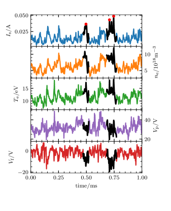
Figure 1: Time series of the ion saturation current, electron density and temperature, and plasma and the floating potentials. Local maxima exceeding 2.5 times the root mean square value of the $I_{\mathrm{s}}$ time series are marked by red dots. The black lines mark $50\,\mu\mathrm{s}$ long sub-records centered around these maxima.

For further analysis of the data time series we rescale them as to have locally vanishing mean and unity variance:

$$\widetilde{\Psi}=\frac{\Psi-{\langle{\Psi}\rangle_{\mathrm{mv}}}}{{{\Psi}_{\mathrm{rms,mv}}}}.$$ (5)

The moving average and moving root mean square time series are computed from samples at $t_{i}=i\triangle_{t}$ as

$${\langle{\Psi}\rangle_{\mathrm{mv}}}(t_{i}) =\frac{1}{2r+1}\sum\limits_{k=-r}^{r}\Psi(t_{i+k}),$$ (6)

$${{\Psi}_{\mathrm{rms,mv}}}(t_{i}) =\left[\frac{1}{2r+1}\sum\limits_{k=-r}^{r}\left(\Psi(t_{i+k})-{\langle{\Psi(t_{i})}\rangle_{\mathrm{mv}}}\right)^{2}\right]^{1/2}.$$ (7)

where $\triangle_{t}=0.3\,\mu\mathrm{s}$ is the sampling time. Using a filter radius $r=16384$, which corresponds to approximately $5\,\mathrm{ms}$, ensures that both the moving average and the moving root mean square time series feature little variation. Indeed, the sample averages of all rescaled time series are approximately $10^{-3}$ and their standard deviations deviates from unity by a comparable factor.

Figure 2 illustrates this rescaling. It shows the $T_{\mathrm{e}}$ time series in physical units in green. The moving average, defined by Eq. ( 6), is shown by the solid black line and flanked by the moving root mean square, shown by the dashed black lines. While the moving root mean square varies little, between $2.5$ and $3.5\,\mathrm{eV}$, the moving sample average varies between $12$ and $19\,\mathrm{eV}$. Absorbing these variations into the normalization of the time series allows to compare samples of the entire one second long data time series.

All rescaled data time series present non-vanishing sample coefficients of skewness and excess kurtosis, or flatness, listed in Tab. 1. While the electron density and temperature time series feature comparable coefficients of skewness, this moment is larger for the ion saturation current. Similarly, the flatness of the ion saturation current time series is consistently larger than for either electron quantity. The floating potential features negative coefficients of sample skewness and non-vanishing coefficients of flatness. On the other hand the plasma potential is skewed towards positive values and also features positive coefficients of sample kurtosis.

Quantity	Skewness	Flatness
$\widetilde{I}_{\mathrm{s}}$	$1.1/1.0/1.2/1.1$	$2.0/1.7/2.5/2.1$
$\widetilde{V}_{\mathrm{f}}$	$-0.23/-0.23/-0.83/-0.64$	$0.031/0.18/0.86/0.66$
$\widetilde{V}_{\mathrm{p}}$	$0.53/0.64/0.76/0.60$	$1.2/1.6/1.9/1.4$
$\widetilde{n}_{\mathrm{e}}$	$0.69$	$0.79$
$\widetilde{T}_{\mathrm{e}}$	$0.63$	$0.88$

Table 1: Sample skewness and flatness of the time series sampled by the southwest / northwest / northeast / southeast MLP ($\widetilde{I}_{\mathrm{s}}$, $\widetilde{V}_{\mathrm{f}}$, $\widetilde{V}_{\mathrm{p}}$) and of the time series averaged over all electrodes ($\widetilde{n}_{\mathrm{e}}$, $\widetilde{T}_{\mathrm{e}}$).

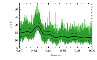
Figure 2: The electron temperature time series (green) and its moving average, defined by Eq. ( 6) (black solid line). The black dashed lines are one moving standard deviation, defined by Eq. ( 7), above and below the moving average.

Compound quantities such as the local electric field and electron particle and heat fluxes are commonly estimated by combining floating potential and ion saturation current measurements. An estimator for the radial electric drift velocity is given by

$$U=\frac{V^{\mathrm{S}}-V^{\mathrm{N}}}{B\triangle_{Z}}.$$ (8)

Here $B=4.1\,\mathrm{T}$ gives the magnetic field at the probe head position, and $(V^{\mathrm{S}}-V^{\mathrm{N}})/\triangle_{Z}$ denotes an estimator for the poloidal electric field. The north and south electrodes of the used probe head are vertically separated by $\triangle_{Z}=2.2\times 10^{-3}\,\mathrm{m}$. In the following we estimate the potential at either poloidal position as the average plasma potential as $V^{\mathrm{N/S}}=(V_{\mathrm{p}}^{\mathrm{NE/SE}}+V_{\mathrm{p}}^{\mathrm{NW/SW}})/2$. Using the plasma potential instead of the floating potential to estimate the electric field includes effects of short-wavelength electron temperature perturbations on the radial velocity. Since toroidal plasma drifts may bias electrodes on the same magnetic flux surface to different electric potentials, the sample mean is subtracted from potential time series used in velocity estimators. Postulating that there is no stationary convection in the scrape-off layer we further subtract the moving average from radial velocity time series such that $\langle\widetilde{U}\rangle_{\mathrm{mv}}=0$.

	$I_{\mathrm{s}}/\mathrm{mA}$	$n_{\mathrm{e}}/10^{18}\mathrm{m}^{-3}$	$T_{\mathrm{e}}/\mathrm{eV}$	$V_{\mathrm{f}}/\mathrm{V}$	$V_{\mathrm{p}}/\mathrm{V}$
Average	$18$	$6.6$	$14$	$1.5$	$38$
rms	$8.7$	$1.8$	$2.7$	$5.5$	$8.2$

Table 2: Lowest order statistical moments of the $I_{\mathrm{s}}$, $V_{\mathrm{f}}$, $V_{\mathrm{p}}$, $T_{\mathrm{e}}$ and $n_{\mathrm{e}}$ data time series.

With fast sampling of the electron density and temperature at hand, the radial electron particle and heat fluxes are estimated as

$$\widehat{\Gamma}_{\mathrm{n}} =\widetilde{n}_{\mathrm{e}}\widetilde{U},$$ (9)

$$\widehat{\Gamma}_{\mathrm{T}} =\frac{{\langle{n_{\mathrm{e}}}\rangle_{\mathrm{mv}}}}{{{n_{\mathrm{e}}}_{\mathrm{rms,mv}}}}\widetilde{T}_{\mathrm{e}}\widetilde{U}+\widetilde{n}_{\mathrm{e}}\frac{{\langle{T_{\mathrm{e}}}\rangle_{\mathrm{mv}}}}{{{T_{\mathrm{e}}}_{\mathrm{rms,mv}}}}\widetilde{U}+\widetilde{n}_{\mathrm{e}}\widetilde{T}_{\mathrm{e}}\widetilde{U}.$$ (10)

Here, $\widetilde{n}_{\mathrm{e}}$, $\widetilde{T}_{\mathrm{e}}$, as well as moving average and moving root mean square time series denote quantities averaged over all four MLPs. This is done as to use all available data of the electron temperature as well as to average out outliers. Table 2 may be used to convert the amplitude of the estimator time series to physical units. We note that Eqs. ( 9) and 10 define fluctuation driven fluxes. The total fluctuation driven heat flux as defined above comprises a conductive contribution, a convective contribution, and a contribution driven by triple correlations.

IV Fluctuation statistics

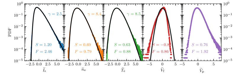
Figure 3: Probability distribution function of the rescaled ion saturation current, the electron density and temperature. Compared are least squares fits of the convolution of a Gamma and a normal distribution (black lines) to the PDFs. The two rightmost panels show the PDFs of the floating potential (red dots) compared to a normal distribution (black line) and of the plasma potential (purple dots).

Figure 3 shows PDFs of the rescaled ion saturation current, the electron density and the electron temperature time series. The two rightmost panels show the PDFs of the floating and the plasma potential. Least squares fits of the convolution of a normal and a Gamma distribution to the PDFs of $\widetilde{I}_{\mathrm{s}}$, $\widetilde{n}_{\mathrm{e}}$, and $\widetilde{T}_{\mathrm{e}}$ are shown by black lines. This distribution arises when assuming that the data time series are due to super-position of uncorrelated exponential pulses with an exponential amplitude distribution and additive white noise, see appendix A in LABEL:theodorsen-2016-php. The shape parameter of this distribution is given by $\gamma=\tau_{\mathrm{d}}/\tau_{\mathrm{w}}$, where $\tau_{\mathrm{d}}$ is the pulse duration time and $\tau_{\mathrm{w}}$ is the average pulse waiting time. Large values of $\gamma$ describe time series that are characterized by significant pulse overlap. Realizations of the process described by Eq. ( 12) with small values of $\gamma$ feature more isolated pulses. The signal to noise ratio of the additional white noise is given by $1/\epsilon$. For small values of $\epsilon$ the signal amplitude is governed by the arrival of exponential pulses, with additive noise contributing little to the signal amplitude.

The PDF of the ion saturation current time series features an elevated tail for large amplitude values. Sample coefficients of skewness and flatness are given by $S=1.2$ and $F=2.5$. A least-squares fit of the prediction by the stochastic model to the PDF yields $\gamma=2.5$ and $\epsilon=3.7\times 10^{-2}$. This fit describes the PDF well over four decades in normalized probability. The PDFs of $\widetilde{n}_{\mathrm{e}}$ and $\widetilde{T}_{\mathrm{e}}$ feature a similar shape but with less elevated tails for large, positive sample values. This is reflected in values of sample skewness and flatness given by $S=0.69$ and $F=0.79$ for $\widetilde{n}_{\mathrm{e}}$ and by $S=0.63$ and $F=0.88$ for $\widetilde{T}_{\mathrm{e}}$. Fitting the prediction by the stochastic model to the PDF of the sampled data yields $\gamma=8.4$ and $\epsilon=0$ for $\widetilde{n}_{\mathrm{e}}$ and $\gamma=8.5$ and $\epsilon=0.13$ for $\widetilde{T}_{\mathrm{e}}$. Again, these parameters suggest a process with significant pulse overlap and little white noise.

Continuing with the PDF of the floating potential we find that negative sample values are more probable then positive sample values. This is reflected by negative value of the sample skewness, $S=-0.83$. The PDF deviates from a normal distribution, shown by the black line in the rightmost panel of Fig. 3, and reflected by a non-vanishing sample flatness $F=0.86$. The PDF of the plasma potential features an elevated tail, similar to the PDF of $\widetilde{T}_{\mathrm{e}}$. On the other hand negative $\widetilde{V}_{\mathrm{p}}$ samples are more probable than negative $\widetilde{T}_{\mathrm{e}}$. Sample skewness and excess kurtosis are both non-vanishing for the plasma potential.

PDFs of $\widetilde{I}_{\mathrm{s}}$ and $\widetilde{V}_{\mathrm{f}}$ recorded by the other MLPs are qualitatively similar to those shown here. Interpreting the PDFs with the relationship given by Eq. ( 1) one may speculate that the elevated tail in the ion saturation current PDF is due to simultaneous large amplitude fluctuations of the electron density and temperature. This issue will be discussed further in the following sections.

Figure 4 shows the power spectral densities (PSDs) of the $\widetilde{I}_{\mathrm{s}}$, $\widetilde{n}_{\mathrm{e}}$, $\widetilde{V}_{\mathrm{p}}$, $\widetilde{V}_{\mathrm{f}}$ and $\widetilde{T}_{\mathrm{e}}$ data time series. They all feature a similar shape, suggesting that fluctuations in the data time series are due to structures with similar characteristic time scales. For $f\lesssim 3\times 10^{-3}\,\mathrm{MHz}$ the PSDs are flat before they roll over to approximately follow a power law, $f^{-2}$, for $3\times 10^{-2}\,\mathrm{MHz}\lesssim f\lesssim 0.1\,\mathrm{MHz}$. For higher frequencies, the PSDs decay even more steep. A least squares fit of Eq. ( 16) to the data gives $\tau_{\mathrm{d}}\approx 15\mu\mathrm{s}$ and $\lambda\approx 0$ for all data time series. The black line gives the curve describe by Eq. ( 16) with just this pulse duration time and vanishing pulse rise time. Equation (16) states that the flat part of the PSD as well as the roll-over frequency is determined by the pulse duration time $\tau_{\mathrm{d}}$. The pulse asymmetry parameter $\lambda$ determines the slope of the PSD after the roll-over. We find that the prediction of the stochastic model with parameters found from least squares fits describe the experimental data well over approximately two decades.

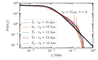
Figure 4: Power spectral density of the ion saturation current, the floating and the plasma potential, and the electron density and temperature. The black line denotes Eq. ( 16) with $\tau_{\mathrm{d}}=15\,\mu\mathrm{s}$.

Figure 5 shows the auto-correlation function for the data time series. The auto-correlation function of $\widetilde{I}_{\mathrm{s}}$, $\widetilde{n}_{\mathrm{e}}$, and $\widetilde{T}_{\mathrm{e}}$ decay approximately exponentially for $\tau\lesssim 20\,\mu\mathrm{s}$. The auto-correlation function of the $\widetilde{V}_{\mathrm{f}}$ and $\widetilde{V}_{\mathrm{p}}$ data time series decay faster than exponential. A least-squares fit of Eq. ( 15) to the data for $\tau<25\,\mu\mathrm{s}$ gives $\tau_{\mathrm{d}}\approx 15\,\mu\mathrm{s}$ and $\lambda\approx 0$ for $\widetilde{I}_{\mathrm{s}}$ and $\widetilde{T}_{\mathrm{e}}$. For $\widetilde{n}_{\mathrm{e}}$ a fit yields $\tau_{\mathrm{d}}\approx 16\,\mu\mathrm{s}$ and a vanishing pulse asymmetry parameter. These parameters agree with the parameters estimated from fits to the PSDs of the data time series.

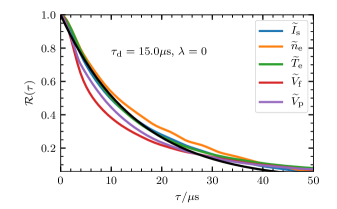
Figure 5: Auto-correlation of the rescaled ion saturation current, electron density and temperature as well as the plasma and the floating potential. Compared is Eq. ( 15) with $\tau_{\mathrm{d}}=15\,\mu\mathrm{s}$ and $\lambda=0$, denoted by the black line.

Figure 6 shows cross-correlation functions between the ion saturation current and the other data time series. The correlation functions $\mathcal{R}_{\widetilde{I}_{\mathrm{s}},\widetilde{n}_{\mathrm{e}}}(\tau)$ and $\mathcal{R}_{\widetilde{I}_{\mathrm{s}},\widetilde{T}_{\mathrm{e}}}(\tau)$ appear similar in shape. They feature maximum correlation amplitudes of approximately $0.75$ at nearly vanishing time lag and are slightly asymmetric, with the correlation amplitude decaying slower for positive than for negative time lags. The cross-correlation function for the plasma potential, $\mathcal{R}_{\widetilde{I}_{\mathrm{s}},\widetilde{V}_{\mathrm{p}}}(\tau)$, features a maximal correlation amplitude of approximately $0.6$ at vanishing time lag. It decays slower to zero for positive time lags than for negative time lags. The cross-correlation function for the floating potential, $\mathcal{R}_{\widetilde{I}_{\mathrm{s}},\widetilde{V}_{\mathrm{f}}}(\tau)$ presents a minimal correlation amplitude of approximately $-0.4$ at $\tau\approx 2\mu\mathrm{s}$. It appears symmetric around the minimum for $-5\mu\mathrm{s}\lesssim\tau\lesssim 8\mu\mathrm{s}$ but decays faster to zero for $\tau>0$ than for $\tau<0$ for large lags. Observing that all auto-correlation functions vanish for time lags greater than $50\,\mu\mathrm{s}$ we note that we do not observe any long-range correlations.

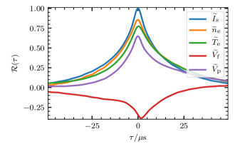
Figure 6: Cross-correlation between all data time series and the ion saturation current.

Complementary to the auto-correlation function we proceed by studying the time series using the conditional averaging method LABEL:pecseli-1989. The conditionally averaged waveform of a signal $\Phi$ is computed by averaging sub-records centered around local maxima of a reference signal $\Psi$ which exceed a threshold value, typically taken to be $2.5$ times the time series root mean square value:

$$\mathcal{C}_{\widetilde{\Phi},\widetilde{\Psi}}(\tau) =\langle\widetilde{\Phi}(\tau)|\widetilde{\Psi}(\tau=0)>2.5,\,\widetilde{\Psi}^{\prime}(0)=0\rangle.$$ (11)

Here the prime denotes a derivative. To ensure that the conditionally averaged waveform is computed from independent samples, the local maxima are required to be separated by the same interval length on which Eq. ( 11) is computed. For the data sets at hand we choose $-25\,\mu\mathrm{s}\leq\tau\leq 25\,\mu\mathrm{s}$.

Figure 7 shows the conditionally averaged waveform of the $\widetilde{I}_{\mathrm{s}}$, $\widetilde{n}_{\mathrm{e}}$, $\widetilde{T}_{\mathrm{e}}$, $\widetilde{V}_{\mathrm{f}}$ and $\widetilde{V}_{\mathrm{p}}$ data time series, using $\widetilde{I}_{\mathrm{s}}$ as a reference signal. Approximately $4000$ maxima are detected in the $\widetilde{I}_{\mathrm{s}}$ time series. The conditionally averaged waveform of the ion saturation current is strongly peaked and decays faster then exponentially to zero for large time lags. The average amplitude of the local ion saturation current maxima is approximately three times the time series root mean square value. The conditionally averaged waveforms of the electron density and temperature are both well approximated by a two-sided exponential function. The maxima of their waveforms are approximately two times the root mean square value of their respective time series. The conditionally averaged waveform of the $\widetilde{V}_{\mathrm{p}}$ time series appears triangular, with the maxima in phase with local maxima of the $\widetilde{I}_{\mathrm{s}}$ time series. The conditionally averaged waveform of the floating potential presents a negative peak with an amplitude of approximately $-1$, occurring at $\tau\approx-2\,\mu\mathrm{s}$. Compared to the averaged waveforms are least square fits of a two-sided exponential waveform, given by Eq. ( 13), to the data, marked by dashed lines in Fig. 7. Table 3 lists their fit parameters. The average waveform duration time is between $12$ and $16\,\mu\mathrm{s}$, comparable to $\tau_{\mathrm{d}}$ estimated by fits to the auto-correlation function and power spectral densities of the signals. The pulse asymmetry parameter for all fits is given by approximately $0.4$.

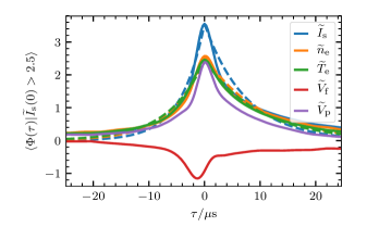
Figure 7: Conditionally averaged waveforms of the data time series, centered around large amplitude maxima in the ion saturation current time series. Dashed lines show least squares fits of a two-sided exponential waveform, given by Eq. ( 13), to the conditionally averaged waveforms.

Waveform	$\langle\widetilde{I}_{\mathrm{s}}|\widetilde{I}_{\mathrm{s}}(0)>2.5\rangle$	$\langle\widetilde{n}_{\mathrm{e}}|\widetilde{I}_{\mathrm{s}}(0)>2.5\rangle$	$\langle\widetilde{T}_{\mathrm{e}}|\widetilde{I}_{\mathrm{s}}(0)>2.5\rangle$
$\tau_{\mathrm{d}}/\mu\mathrm{s}$	$11$	$16$	$16$
$\lambda=\tau_{\mathrm{r}}/\tau_{\mathrm{d}}$	$0.37$	$0.37$	$0.40$

Table 3: Duration time of the last squares fits shown in Fig. 7 and the waveform asymmetry parameter $\lambda$.

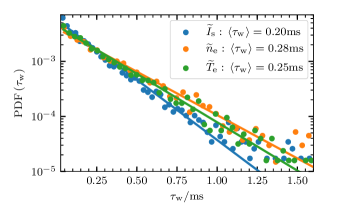
Figure 8: PDFs of the waiting times between large-amplitude bursts in the $n_{\mathrm{e}}$, $T_{\mathrm{e}}$, and $I_{\mathrm{s}}$ time series, recorded by the southwest MLP. The full lines show PDFs of a truncated exponential distribution with a scale parameter given by a maximum likelihood estimate to the data points.

Computing the time lag between successive, conditional maxima of the time series yields the waiting time statistics for large-amplitude events. Figure 8 shows the waiting time PDF of the $\widetilde{I}_{\mathrm{s}}$, $\widetilde{n}_{\mathrm{e}}$ and $\widetilde{T}_{\mathrm{e}}$ time series. Compared are PDFs of exponentially distributed variables. Their scale parameter is given by a maximum likelihood estimate of the waiting time distribution. The resulting distributions describe the data well over approximately two decades in probability. Average waiting times are given by approximately $0.25\,\mathrm{ms}$ for $\widetilde{T}_{\mathrm{e}}$ and $0.28\,\mathrm{ms}$ for $\widetilde{n}_{\mathrm{e}}$. The average waiting time between large-amplitude bursts in $\widetilde{I}_{\mathrm{s}}$ is approximately $0.20\,\mathrm{ms}$. We note that the exact numerical values depend slightly on the threshold value and the conditional window length used.

The PDFs of the signals local maxima are shown in Fig. 9. As for the average waiting times, the PDFs are well described by a truncated exponential distribution. The scale parameter, found by maximum likelihood estimates of the data, are given by $\langle A\rangle\approx 1.0$ for $\widetilde{I}_{\mathrm{s}}$, $\langle A\rangle\approx 0.77$ for $\widetilde{n}_{\mathrm{e}}$, and by $\langle A\rangle\approx 0.83$ for $\widetilde{T}_{\mathrm{e}}$. Given the threshold amplitude of $2.5$, this translates to an average burst amplitude of the rescaled signals between $3.3$ and $3.5$ times the root-mean-square value of the data time series, consistent with the amplitude of the conditionally averaged waveforms shown in Fig. 9.

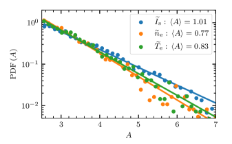
Figure 9: PDF of large amplitude local maxima in the rescaled time series. Full lines show the PDFs of a truncated exponential distribution with a scale parameter given by a maximum likelihood estimate to the data time series.

V Radial velocity and fluxes

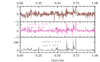
Figure 10: Estimators for the radial velocity (upper panel) and the radial electron particle, and heat flux (middle and lower panel). The full (dashed) line in the upper panel denotes the radial velocity estimated from $V_{\mathrm{p}}$ ($V_{\mathrm{f}}$) samples. The full (dashed) line in the middle panel denotes the radial electron flux esimated from $\widetilde{n}_{\mathrm{e}}$ and $\widetilde{U}_{V_{\mathrm{p}}}$ ($\widetilde{I}_{\mathrm{s}}$ and $\widetilde{U}_{V_{\mathrm{f}}}$) samples. The time interval is identical to the one presented in Fig. 1.

In the following the statistical properties of the radial velocity and electron particle and heat fluxes are discussed. Figure 10 shows $1\,\mathrm{ms}$ long time series of the estimators given by Eqs. ( 8) - (10), computed on the same time interval as the time series shown in Fig. 1. The full (dashed) line in the upper panel denotes the radial velocity estimated from $V_{\mathrm{p}}$ ($V_{\mathrm{f}}$) samples. In the middle panel the full (dashed) line denotes the radial electron flux estimated from $n_{\mathrm{e}}$ and $V_{\mathrm{p}}$ ($I_{\mathrm{s}}$ and $V_{\mathrm{f}}$) samples. The radial velocity time series show fluctuations on a similar time scale as seen for the time series shown in Fig. 1. There is no qualitative difference between $\widetilde{U}$ estimated from the floating potential and from the plasma potential. Both positive and negative local maxima appear with nearly equal frequency, not exceeding $5$ in normalized units. The $\widehat{\Gamma}_{\mathrm{n}}$ time series feature predominantly positive fluctuation amplitudes on a similar temporal scale as the $\widetilde{U}$ time series. Using ion saturation current and floating potential to estimate the particle flux yields almost indistinguishable estimator samples. The sample mean and root mean square value are given by $0.42$ ($0.48$) and $1.25$ ($1.20$) respectively, using $n_{\mathrm{e}}$ and $V_{\mathrm{p}}$ ($I_{\mathrm{s}}$ and $V_{\mathrm{f}}$) samples. The radial heat flux time series $\widehat{\Gamma}_{\mathrm{T}}$ features large-amplitude bursts exceeding $80$ in normalized units. Large-amplitude temperature fluctuations, which appear in phase with large-amplitude particle flux events, give rise to this large fluctuation level. Only few large, negative heat flux events are recorded.

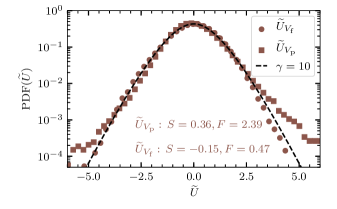
Figure 11: PDF of the rescaled radial electric drift velocity. Compared is the PDF predicted from the stochastic model, given by Eq.(A9) LABEL:theodorsen-2016-ppcf, for a Laplace distribution of pulse amplitudes.

Figure 11 presents the PDF of the radial velocity estimator given by Eq. ( 8). The PDF of $\widetilde{U}_{\widetilde{V}_{\mathrm{f}}}$ appears symmetric with exponential tails for both positive and negative sample values, compatible with $S=-0.15$ and $F=0.47$. The PDF of $\widetilde{U}_{\widetilde{V}_{\mathrm{p}}}$ is almost identical to the PDF computed using floating potential measurements, but notably features an elevated tail for large amplitude samples $\widetilde{U}_{\widetilde{V}_{\mathrm{p}}}\gtrsim 2.5$. A correlation analysis of samples $V_{\mathrm{f}}^{\mathrm{S}}-V_{\mathrm{f}}^{\mathrm{N}}$ and $T_{\mathrm{e}}^{\mathrm{S}}-T_{\mathrm{e}}^{\mathrm{N}}$ showed no correlation between large-amplitude potential differences to large amplitude electron temperature differences, which may have explained this artifact in the PDF. The coefficient of sample skewness for $\widetilde{U}_{\widetilde{V}_{\mathrm{f}}}$ is slightly negative, while the elevated tail of $\mathrm{PDF}(\widetilde{U}_{\widetilde{V}_{\mathrm{p}}})$ yields a slightly positive coefficient of sample skewness. Compared to the PDF is the probability distribution function of the process defined by Eq. ( 12) with Laplace distributed pulse amplitudes, which allows for positive as well as negative pulse amplitudes LABEL:theodorsen-2016-ppcf,_theodorsen-2018-ppcf. Estimating $\gamma$ by a least squares fit to the PDF of $\widetilde{U}_{\widetilde{V}_{\mathrm{f}}}$ yields $\gamma\approx 10$. This value is comparable with the intermittency parameter for the $\widetilde{n}_{\mathrm{e}}$ and $\widetilde{T}_{\mathrm{e}}$ data time series and is larger by a factor of approximately 4 than for the $\widetilde{I}_{\mathrm{s}}$ time series.

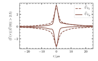
Figure 12: Conditionally averaged waveform of local extrema in the radial velocity time series.

The auto-conditionally averaged waveform of large-amplitude velocity fluctuations, computed from approximately $3000$ events, are shown in Fig. 12. The average waveform is approximately triangular for the $\widetilde{U}_{\widetilde{V}_{\mathrm{p}}}$ time series while it is less peaked for the $\widetilde{U}_{\widetilde{V}_{\mathrm{f}}}$ time series. The duration time of both waveforms is approximately $5\,\mu\mathrm{s}$, smaller by a factor of three than the conditionally averaged waveforms of the electron density and temperature.

The PDF of the waiting times between local extrema in the $\widetilde{U}$ time series, both positive and negative, are shown in Fig. 13. Compared are PDFs of exponentially distributed variables with scale parameters given by $\langle\tau_{\mathrm{w}}\rangle=0.08\,\mathrm{ms}$ for $\widetilde{U}_{\widetilde{V}_{\mathrm{p}}}$ and by $\langle\tau_{\mathrm{w}}\rangle=0.13\,\mathrm{ms}$ for $\widetilde{U}_{\widetilde{V}_{\mathrm{f}}}$. These parameters have been estimated by a maximum likelihood estimate of the respective waiting time data. The resulting distributions describes the waiting times well over approximately two decades in probability. Varying the minimum separation between detected local extrema changes the average waiting time only little since positive and negative maxima are detected independently of each other.

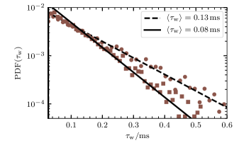
Figure 13: PDF of the waiting times between successive, positive or negative, extrema in the radial velocity time series. Square (circle) plot markers denote the radial velocity estimated from $V_{\mathrm{p}}$ ($V_{\mathrm{f}}$) samples. Compared are exponential distributions with a scale parameter given by a maximum likelihood estimate of the waiting times.

The PDF of the local extrema is shown in Fig. 14. Compared to the positive and negative legs of the distribution are truncated exponential distributions for $|A|>2.5$. Each distribution has been multiplied by $1/2$ to normalize the integral of both PDFs to unity. A least squares fit to the $\widetilde{U}_{\widetilde{V}_{\mathrm{p}}}$ data yields a scale parameter of approximately $1$ for both positive and negative amplitudes. Together with the result that the waiting times between large local maxima of the velocity time series are well described by an exponential distribution, these findings corroborate the hypothesis to interpret the radial velocity time series as a super-position of uncorrelated pulses described by Eq. ( 12).

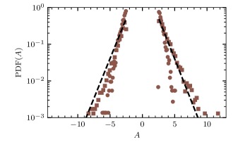
Figure 14: PDF of the local maxima in the radial velocity time series. Square (circle) plot markers denote the radial velocity estimated from $V_{\mathrm{p}}$ ($V_{\mathrm{f}}$) samples. Compared are fits on exponential distribution multiplied by a factor $1/2$, for $A>2.5$ and $A<2.5$.

Figure 15 presents the PDF of the radial particle fluxes computed using either $n_{\mathrm{e}}$ and $V_{\mathrm{p}}$ samples or $I_{\mathrm{s}}$ and $V_{\mathrm{f}}$ samples. The PDFs are almost indistinguishable. They are strongly peaked at zero and feature non-exponential tails for both positive and negative sample values. Positive sample values have a much higher probability than negative sample values. This is reflected by coefficients of sample skewness and excess kurtosis given by $S=4.3$ ($3.8$) and $F=65$ ($33$), respectively.

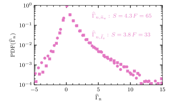
Figure 15: PDF of the normalized radial electron flux. Square (circle) plot markers denote the radial electron flux estimated using $\widetilde{n}_{\mathrm{e}}$ and $U_{V_{\mathrm{p}}}$ ($\widetilde{I}_{\mathrm{s}}$ and $U_{V_{\mathrm{f}}}$) samples.

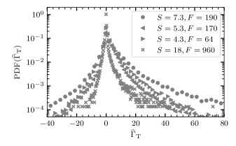
Figure 16: PDF of the total radial heat flux (circle), the conductive (triangle left), convective heat fluxes (triangle right), and the heat flux due to triple correlations(cross).

The PDF of the radial heat flux, shown by circles in Fig. 16, presents a similar shape with heavy tails for large sample values. Sample coefficients of skewness and flatness are given by $S=7.3$ and $F=190$. Also shown are PDFs of the conductive heat flux $({\langle{n_{\mathrm{e}}}\rangle_{\mathrm{mv}}}/{{n_{\mathrm{e}}}_{\mathrm{rms,mv}}})\,\widetilde{T}_{\mathrm{e}}\,\widetilde{U}$ (triangle left), the convective heat flux, $\widetilde{n}_{\mathrm{e}}({\langle{T_{\mathrm{e}}}\rangle_{\mathrm{mv}}}/{{T_{\mathrm{e}}}_{\mathrm{rms,mv}}})\,\widetilde{U}$ (triangle right), and triple correlations $\widetilde{n}_{\mathrm{e}}\,\widetilde{T}_{\mathrm{e}}\,\widetilde{U}$ (cross). PDFs of the conductive and convective heat fluxes appear similar in shape as the total heat flux. However, large-amplitude convective heat flux samples occur more frequently than conductive heat flux samples of equal magnitude. The PDF of the heat flux due to triple correlations is strongly peaked for small amplitudes and skewed towards positive sample values.

	$\Gamma_{n}$	$\Gamma_{T}$	${\langle{n_{\mathrm{e}}}\rangle_{\mathrm{mv}}}\,\widetilde{T}_{\mathrm{e}}\,\widetilde{U}$	${\langle{T_{\mathrm{e}}}\rangle_{\mathrm{mv}}}\,\widetilde{n}_{\mathrm{e}}\,\widetilde{U}$	$\widetilde{n}_{\mathrm{e}}\,\widetilde{T}_{\mathrm{e}}\,\widetilde{U}$
Average $10^{20}\,\mathrm{m}^{-2}\mathrm{s}^{-1}$	$2.9$	$70\,\mathrm{eV}$	$27\,\mathrm{eV}$	$39\,\mathrm{eV}$	$4.2\,\mathrm{eV}$
Root mean square $10^{20}\,\mathrm{m}^{-2}\mathrm{s}^{-1}$	$8.8$	$250\,\mathrm{eV}$	$95\,\mathrm{eV}$	$120\,\mathrm{eV}$	$55\,\mathrm{eV}$

Table 4: Sample average and root mean square value of the contributions to the radial fluxes.

The sample averages and root mean square values of the various contributions to the total heat flux are listed in Tab. 4. This data shows that $38\%$ of the total fluctuation driven heat flux is due to conduction, $56\%$ due to convection, and $6\%$ due to triple correlations. For both the particle and the total heat flux we find that their root mean square value is approximately two-three times their mean value. This also holds for the conductive and the convective heat fluxes. The relative fluctuation level of the heat flux due to triple correlations is approximately 12.

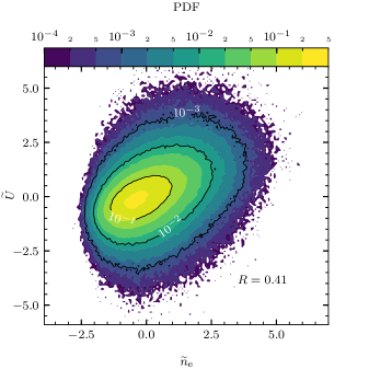
Figure 17: Joint PDF of the radial velocity and the electron density fluctuations.

We continue by discussing the correlations between the electron density and temperature and the radial velocity fluctuation time series. Figure 17 presents the joint PDF of the fluctuating radial velocity and electron density. The linear sample correlation coefficient is given by $R=0.41$, consistent with the slightly tilted shape of the ellipsoids capturing probabilities less than $10^{-1}$, $10^{-2}$ and $10^{-3}$. Large-amplitude fluctuations are enclosed by equi-probability ellipsoids whose semi-minor axis increases with decreasing probability. Negative large-amplitude velocity fluctuations, $\widetilde{U}\lesssim-2.5$, appear in phase with small positive and negative density fluctuations. Positive, large amplitude density fluctuations, $\widetilde{n}_{\mathrm{e}}\gtrsim 2.5$, appear on average in phase with positive velocity fluctuations. Negative density fluctuations appear on average with vanishing velocity fluctuations while positive velocity fluctuations, $\widetilde{U}\gtrsim 2.5$ appear on average in phase with positive density fluctuations.

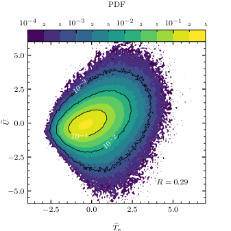
Figure 18: Joint probability distribution function of the radial velocity and electron temperature fluctuations.

The joint PDF of the fluctuating radial velocity and the electron temperature, shown in Fig. 18, features some qualitative similarities to the joint PDF of the velocity and density fluctuations. Small-amplitude fluctuations are correlated, captured by a tilted ellipsoid for a joint probability approximately less than $0.1$. The sample correlation coefficient for the time series is given by $R=0.29$. Large-amplitude fluctuations are captured by equi-probability contours whose shape increasingly deviates from an ellipse with decreasing probability. Especially are large, negative velocity fluctuations observed which are in phase with small, positive temperature fluctuations. Large negative temperature fluctuations are in phase with small velocity fluctuations, $\widetilde{U}\approx 0$, with less scatter than observed for the density fluctuations. Large positive temperature fluctuations are on average in phase with positive temperature fluctuations, also with larger scatter than observed for the density fluctuations. Large velocity fluctuations with $\widetilde{U}\gtrsim 2.5$ are correlated with positive temperature fluctuations. Similar to the correlation to density fluctuations, are large negative velocity fluctuations, $\widetilde{U}\lesssim 2.5$ on average in phase with small, positive temperature fluctuations.

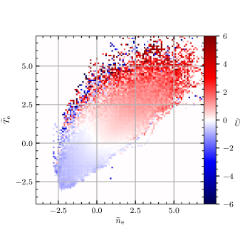
Figure 19: Amplitude of the velocity fluctuations as a function of the electron density and temperature fluctuation amplitude.

Figure 19 presents the radial velocity amplitudes encoded in a scatter plot of the electron density and temperature fluctuations. Large-amplitude velocity fluctuations are in phase with large-amplitude fluctuations in both electron temperature and density. The magnitude of $\widetilde{U}$ increases with the amplitude of $\widetilde{n}_{\mathrm{e}}$ and $\widetilde{T}_{\mathrm{e}}$. Few negative velocity fluctuations are observed for $\widetilde{n}_{\mathrm{e}}\gtrsim 0$ and $\widetilde{T}_{\mathrm{e}}\gtrsim 0$. Negative velocity fluctuations are observed for $\widetilde{n}_{\mathrm{e}}\gtrsim 0$ and $\widetilde{T}_{\mathrm{e}}\lesssim 0$, as well as for $\widetilde{T}_{\mathrm{e}}\gtrsim 0$ and $\widetilde{n}_{\mathrm{e}}\lesssim 0$.

We continue by investigating how these fluctuations contribute to the radial heat flux. For this we present the conditionally averaged wave forms of the fluctuating time series, centered around heat flux events exceeding $25$ in normalized units, shown in Fig. 20. Here we use the conductive and convective heat flux, as well as contributions from triple correlations as reference signals. The left panels show the conditionally averaged waveforms of the respective heat fluxes and the right panels show their conditional variance (CV) LABEL:oynes-1995. The conditional variance describes the average deviation of the individual waveforms from the average waveform. A value of $\mathrm{CV}=0$ describes identical individual waveforms while a value of $\mathrm{CV}=1$ describes random individual waveforms. In total $2692$ local maxima are identified in the conductive heat flux time series, $3963$ in the convective heat flux time series and $992$ in the triple correlations time series. These counts agree with the PDFs of individual heat flux contributions, shown in Fig. 16, where the same ordering of the sample probabilities holds for large amplitude fluctuations.

Using the conductive heat flux as a reference signal we find that its auto-conditionally averaged waveform appears triangular and is reproducible with $\max 1-\mathrm{CV}$ approximately $1$. The average waveform of the electric drift velocity appears similar in shape while the average waveform of the electron density and temperature fluctuations present a broad shape with a fast rise and slow decay. Temperature and velocity fluctuations which mediate conductive heat flux events appear highly reproducible. The slower decay time scale of the temperature fluctuations mediating these heat flux events ($\tau_{\mathrm{d}}\approx 15\mu\mathrm{s}$) appears reproducible among the individual events, as suggested by the slowly decreasing conditional variance for $\tau>0$. Density and velocity fluctuations, which constitute convective heat flux events present on average a qualitatively similar shape, although with an average amplitude smaller by a factor of $1.5$. Their average waveform also appears more random than their average waveform for conductive heat flux events. Here we find $\max 1-\mathrm{CV}\approx 0.6$ for $\widetilde{n}_{\mathrm{e}}$ and $\max 1-\mathrm{CV}\approx 0.7$ for $\widetilde{U}$. As for the conductive heat flux, the average density and temperature fluctuations associated with convective heat flux events present less variance for $\tau>0$ than for $\tau<0$. Conditionally averaged waveforms of the density, temperature, and velocity fluctuations associated with large-amplitude triple correlation heat flux events are qualitatively similar to the two previous cases. The average velocity waveform appears similar to the average heat flux waveform. The average density and temperature waveform features a fast rise and a slow decay. Their slower decay is robustly reproducible by all individual density and temperature waveforms.

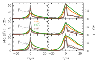
Figure 20: Conditionally averaged waveform of the electron density and temperature and the radial velocity during heat flux bursts (left panels). The right panels shows the conditional variance of the waveforms.

VI Discussion

The data time series of the ion saturation current, the electron density, and the electron temperature have similar statistical properties. They all feature large-amplitude, intermittent bursts on a similar time scale. However, the relative fluctuation level of the $I_{\mathrm{s}}$ data is approximately twice as large as those of the $n_{\mathrm{e}}$ and $T_{\mathrm{e}}$ data. Furthermore the PDF of $\widetilde{I}_{\mathrm{s}}$ features higher probabilities for large-amplitude fluctuations than PDFs of $\widetilde{n}_{\mathrm{e}}$ and $\widetilde{T}_{\mathrm{e}}$. Sample skewness and flatness of the $\widetilde{I}_{\mathrm{s}}$ time series are approximately $1.5-2$ times larger than for the $\widetilde{n}_{\mathrm{e}}$ and $\widetilde{T}_{\mathrm{e}}$ time series. This tendency of the $I_{\mathrm{s}}$ data to deviate strongly from the sample mean may be explained by the correlation of the $n_{\mathrm{e}}$ and $T_{\mathrm{e}}$ sample amplitude. According to Eq. ( 1) correlated large-amplitude $n_{\mathrm{e}}$ and $T_{\mathrm{e}}$ samples increase the ion saturation current significantly.

Relative fluctuation levels of the electron density and temperature are given by $0.27$ and $0.19$ respectively. Similar values have been reported from the TEXT-U tokamak LABEL:meier-2001. The ion saturation current samples feature a relative fluctuation level of $0.47$. A lower relative fluctuation level of $T_{\mathrm{e}}$ compared to $I_{\mathrm{s}}$ was also reported from ASDEX Upgrade LABEL:horacek-2010. Coefficients of sample skewness and excess kurtosis are given by $S=0.69$ and $F=0.79$ for $\widetilde{n}_{\mathrm{e}}$ and by $S=0.63$ and $F=0.88$ for $\widetilde{T}_{\mathrm{e}}$. These values are similar in magnitude to values reported from the SINP tokamak LABEL:saha-2008. We note that the particular numerical value of the time series statistics depends weakly on the width of the applied running average filter and weakly on whether the time series are averaged over the MLP electrodes. However, the conclusion that electron density and temperature time series present large-amplitude, intermittent bursts, with skewed, non-Gaussian PDFs, is independent of the data preprocessing.

These observations motivate to interpret the $I_{\mathrm{s}}$, $n_{\mathrm{e}}$, and $T_{\mathrm{e}}$ data time series as a realization of the stochastic process described by Eq. ( 12). Indeed, the time series are well described by a Gamma distribution. A least squares fit to the PDF predicted by the stochastic model LABEL:theodorsen-2016-ppcf,_theodorsen-2017-ps yields shape parameters of $\gamma=2.5$ for $\widetilde{I}_{\mathrm{s}}$ as well as $\gamma=8.4$ and $\gamma=8.5$ for $\widetilde{n}_{\mathrm{e}}$ and $\widetilde{T}_{\mathrm{e}}$ respectively. The shape parameter agrees well with results from previous analysis of the ion saturation current in Alcator C-Mod, taken with conventional Langmuir probes LABEL:kube-2016-ppcf. On the other hand, PDFs of scrape-off layer fluctuations at the limiter radius, measured by the GPI diagnostic, are more skewed towards positive values and present a shape parameters closer to unity LABEL:garcia-2013. This disparity may be attributed to the fact that GPI is sensitive to both the electron density and temperature. Furthermore may burnouts, where hot blobs ionize neutral atoms, locally decrease the measured GPI intensity level LABEL:zweben-2002,_stotler-2003.

Intermittent, large-amplitude fluctuations of the electron density and temperature may have consequences for the life-time of the plasma facing components (PFCs) LABEL:marandet-2016. A Debye sheath at the vacuum vessel wall accelerates ions from the plasma onto the PFCs. Assuming that the ion temperature is equal to the electron temperature, ions impact onto the PFCs with an energy approximately five times the electron temperature LABEL:naujoks-book. Such processes are often quantified by the sputtering yield $Y$, which gives the ratio of emitted target particle per incident. The sputtering yield is computed with the Bohdansky formula LABEL:bohdansky-1984 which depends non-linearly on the impact particle energy and on material properties of the target. Using the average temperature values reported here, yields a vanishing sputtering yield, $Y(\langle E\rangle)=0$. Using the fact that the impact ions are Gamma distributed with a shape parameter $\gamma=8.5$ we find $\langle Y(E)\rangle=5.4\times 10^{-5}$ for the Molybdenum walls installed in Alcator C-Mod. For lighter materials such as Beryllium, the used distribution results in average sputtering yields larger by approximately three orders of magnitude.

The fluctuation amplitudes in the $\widetilde{n}_{\mathrm{e}}$ and $\widetilde{T}_{\mathrm{e}}$ time series, as well as the waiting times between them are well described by an exponential distribution. The conditionally averaged waveform of local maxima is well approximated by a two-sided exponential function with a duration time of approximately $15\,\mu\mathrm{s}$. Similar conditionally averaged waveforms of electron density and temperature fluctuations have been reported from DIII-D LABEL:boedo-2003,_rudakov-2005. Measurements from ASDEX upgrade, suggesting a dip in the conditionally averaged temperature waveform LABEL:horacek-2010, are not confirmed by our analysis.

The power spectral densities of the $\widetilde{n}_{\mathrm{e}}$ and $\widetilde{T}_{\mathrm{e}}$ time series agrees well with the PSD predicted by the stochastic model. Estimating the duration time by a least squares fit of Eq. ( 16) to the data yields duration times of approximately $15\,\mu\mathrm{s}$, comparable to the estimated duration time from fits to the conditionally averaged waveform. On the other hand a fit to the PSD yields an asymmetry parameter $\lambda=0$ while conditional averaging yields $\lambda=0.4$. This discrepancy is likely due to significant overlap of the pulses in the data time series, as suggested by $\gamma=\tau_{\mathrm{d}}/\tau_{\mathrm{w}}\approx 10$ from Fig. 3 LABEL:garcia-2012. Thus there are on average several pulses within a given conditional averaging window which smear out the conditionally averaged waveform.

The PDF of the $\widetilde{V}_{\mathrm{p}}$ time series is skewed towards positive values. Given the sample correlation coefficient of this time series and the $\widetilde{T}_{\mathrm{e}}$ time series, $R_{V_{\mathrm{p}},T_{\mathrm{e}}}=0.77$, this suggests that the plasma potential is governed by the electron temperature. A comparison of velocity and flux estimators using the density and plasma potential data to the ”classical” ion saturation current and floating potential data suggests however that this effect has no significant consequences. The radial velocity estimates using either potential variable feature similar sample statistics, as shown in Fig. 11. Particle flux samples computed from $n_{\mathrm{e}}$ and $V_{\mathrm{p}}$ data are almost indistinguishable from samples computed using $I_{\mathrm{s}}$ and $V_{\mathrm{f}}$ data, as shown in Fig. 15.

The velocity time series has similarities to the electron density and temperature time series - it features intermittent, large-amplitude deviations from the sample mean. Large amplitude deviations are however both positive and negative. The PDF of the time series is therefore symmetric. It also features exponential tails for large amplitude events $|\widetilde{U}|\gtrsim 2.5$. Generalizing the stochastic model to include Laplace distributed amplitudes yields an analytic expression for the PDF which describes the data time series over more than 3 orders of magnitude in probability. The average pulse duration in the $\widetilde{U}$ data, $5\,\mu\mathrm{s}$, is three times smaller than the pulse duration time in the electron density and temperature time series. The shape parameter of the PDF is given by $10$, comparable to the shape parameter that best describes the PDF of the $\widetilde{n}_{\mathrm{e}}$ and $\widetilde{T}_{\mathrm{e}}$ data.

A correlation analysis of the large-amplitude fluctuations in the electron density, temperature, and velocity time series shows that a large fraction of them are in phase. Density and velocity fluctuations that appear in phase lead to large particle flux events. This may explain the elevated tail of the PDF of $\widehat{\Gamma}_{n}$, show in Fig. 15. PDFs with similar shapes have been observed for scrape-off layer plasmas LABEL:xu-2005,_garcia-2006-tcv,_garcia-2007-nf,_fedorczak-2011,_kube-2016-ppcf as well as in numerical simulations of scrape-off layer plasmas LABEL:ghendrih-2003,_ghendrih-2005,_garcia-2008-ppcf. Analysis of measurements taken in TEXT-U also report a strong correlation between density and temperature fluctuations LABEL:meier-2001. Figure 19 suggests a similar strong correlation between $\widetilde{n}_{\mathrm{e}}$ and $\widetilde{T}_{\mathrm{e}}$ in our time series. This figure furthermore suggests that a fraction of the large-amplitude fluctuations in all three quantities are correlated. These can be interpreted as dense and hot plasma blobs.

This is compatible with the theory that the radial motion of plasma blobs is governed by the interchange mechanism. Fluid models, often employed to describe blob dynamics, suggest that the radial blob velocity is determined by the poloidal electron pressure gradient within the blob structure LABEL:krash-2001,_bian-2003,_garcia-2006. Numerical simulations of such models find a dipolar potential structure aligned with the pressure gradient. While the dipole is out of phase with the pressure perturbation the resulting electric drift is in phase with the pressure perturbation. The resulting electric dipole structure has been reported from floating potential measurements in tokamak plasmas LABEL:rudakov-2002,_grulke-2006,_kube-2016-ppcf,_theodorsen-2016-ppcf and basic plasma experiments LABEL:katz-2008,_furno-2011,_theiler-2011. Numerical simulations of blobs including dynamic finite Larmor radius effects present dipolar potential stratifications along the pressure gradient of a plasma blob LABEL:wiesenberger-2014,_held-2016. Furthermore numerical simulations of blobs, electrically connected to sheaths formed at the divertor, show a regime where a mono-polar potential structure within a blob results in an intrinsic blob spin LABEL:myra-2004,_dippolito-2004. The observed mono-polar dip associated with large-amplitude electron density maxima is thus inconclusive about whether a single physical mechanism governs blob propagation.

The radial electron heat flux time series features a relative fluctuation level of approximately three and non-gaussian statistics, skewed towards large-amplitude events. The conductive and convective heat fluxes contribute $94\%$ to the total fluctuation driven heat flux. Furthermore is their respective relative fluctuation level approximately the same as that of the total heat flux. As shown in the joint PDFs of $\widetilde{U}$, $\widetilde{n}_{\mathrm{e}}$, and $\widetilde{T}_{\mathrm{e}}$, see Figs. 17 and 18, and the conditional average analysis in Fig. 20, is there slightly more scatter in the convective heat flux than in the conductive heat flux. Triple correlations contributing on average approximately $6\%$ to the total heat flux. The large relative fluctuation level of this contribution to the total flux, approximately $13$, is due to the few number of events where large-amplitude fluctuations of $\widetilde{U}$, $\widetilde{n}_{\mathrm{e}}$, and $\widetilde{T}_{\mathrm{e}}$ are in phase, as shown in Figs. 16 and 19.

VII Conclusions

Plasma fluctuations in the out board mid-plane scrape-off layer plasma in an ohmically heated, lower single-null diverted discharge in Alcator C-Mod have been analyzed. One second long data time series were sampled using Mirror Langmuir probes, dwelling at the outboard mid-plane limiter position. Time series of the electron density and temperature as well as the ion saturation current present intermittent, large-amplitude bursts. Large-amplitude fluctuations in the ion saturation current appear more frequently than similar large-amplitude fluctuations in the electron density and temperature time series. Large-amplitude $n_{\mathrm{e}}$ and $T_{\mathrm{e}}$ fluctuations appear in phase. This leads to increased $I_{\mathrm{s}}$ samples compared to attributing them solely to electron density fluctuations. Both $\widetilde{n}_{\mathrm{e}}$ and $\widetilde{T}_{\mathrm{e}}$ are shown to be well described by the stochastic process given by Eq. ( 12). We find furthermore that the velocity fluctuations can be described by a similar stochastic process by allowing for both negative and positive fluctuation amplitudes. The particle and heat flux towards the outboard mid-plane limiter structure appear intermittent and are driven by fluctuations in both the electron density and temperature. Both conductive and convective heat feature a similar PDF and contribute respectively approximately $56$ and $38$ percent to the total heat flux. Hot and dense plasma blobs contribute to the heat flux via triple correlations, albeit on average approximately $6$ percent. Accounting for the observed fluctuations of the electron temperature shows that large heat flux events contribute to sputtering of the plasma facing components.

Future work will focus on exploring the fluctuation statistics for various plasma parameters as well as analysis on fluctuations sampled by divertor probes.

Appendix A Stochastic Model

For an interpretation of the data time series we employ the stochastic model developed in Refs. LABEL:garcia-2012,_theodorsen-2016-ppcf,_garcia-2016,_garcia-2017-ac. Within this framework time series are modeled as the super-position of uncorrelated pulses,

$$\Phi(t)=\sum\limits_{k=1}^{K(T)}A_{k}\varphi\left(\frac{t-t_{k}}{\tau_{\mathrm{d}}}\right).$$ (12)

Here $K(T)$ gives the number of pulses arriving in the time interval $[0:T]$, $A_{k}$ gives the amplitude of the $k$-th pulse and $t_{k}$ its arrival time. A universal pulse shape is given by $\varphi(\theta)$ and $\tau_{\mathrm{d}}$ gives the characteristic time scale of the pulses.

Motivated by measurements in scrape-off layer plasmas LABEL:boedo-2003,_antar-2003,_garcia-2006-tcv,_garcia-2007-nf,_horacek-2010,_garcia-2013,_garcia-2015,_militello-2013,_carralero-2014 and numerical simulations LABEL:garcia-2006-tcv,_garcia-2007-nf we assume that the pulse amplitudes are exponentially distributed and that all pulses present the same pulse shape. We also assume that pulse arrivals are governed by a Poisson process where $K$ pulses arrive in a time interval $[0:T]$ with an average waiting time $\tau_{\mathrm{w}}$. The ratio of the pulses duration time and the average waiting time between pulses $\gamma=\tau_{\mathrm{d}}/\tau_{\mathrm{w}}$ is referred to as the intermittency parameter. Realizations of Eq. ( 12) with significant pulse overlap are described by large values of $\gamma$, while realizations of Eq. ( 12) with little pulse overlap are described by a small value of $\gamma$.

Based on the same observations we postulate that the average pulse shape is described by a two-sided exponential function

$$\varphi(\tau)=\begin{cases}\displaystyle{\exp\left(\frac{\tau}{\tau_{\mathrm{r}}}\right)}\quad&\mathrm{for}\,\tau<0,\\ \displaystyle{\exp\left(-\frac{\tau}{\tau_{\mathrm{f}}}\right)}\quad&\mathrm{for}\,\tau\geq 0.\\ \end{cases}$$ (13)

The pulse duration time is given by the sum of the rise and fall e-folding times, $\tau_{\mathrm{d}}=\tau_{\mathrm{r}}+\tau_{\mathrm{f}}$, and a pulse asymmetry parameter is defined as $\lambda=\tau_{\mathrm{r}}/\tau_{\mathrm{d}}$. Under these assumptions the process described by Eq. ( 12) is Gamma distributed LABEL:garcia-2012,

$$P_{\Phi}(\Phi)=\frac{1}{\langle\Phi\rangle\Gamma(\gamma)}\left(\frac{\Phi}{\langle\Phi\rangle}\right)^{\gamma-1}\exp\left(-\frac{\Phi}{\langle\Phi\rangle}\right),$$ (14)

where $\langle\cdot\rangle$ denotes an ensemble average. The shape parameter of the PDF is given by the intermittency parameter $\gamma$ and is notably independent of $\lambda$ and $\tau_{\mathrm{d}}$.

The auto-correlation function of the normalized process $\widetilde{\Phi}=\left(\Phi-\langle\Phi\rangle\right)/\Phi_{\mathrm{rms}}$ is given by LABEL:theodorsen-2016-ppcf,_garcia-2016,_garcia-2017-ac

$$\mathcal{R}_{\widetilde{\Phi}}(\tau)=\frac{\tau_{\mathrm{f}}e^{-|\tau|/\tau_{\mathrm{f}}}-\tau_{\mathrm{r}}e^{-|\tau|/\tau_{\mathrm{r}}}}{\tau_{\mathrm{f}}-\tau_{\mathrm{r}}}.$$ (15)

This geometrical average approaches an exponential decay in the limit of large pulse asymmetry, $\tau_{\mathrm{r}}\ll\tau_{\mathrm{f}}$ or $\tau_{\mathrm{f}}\ll\tau_{\mathrm{r}}$. For nearly symmetric pulses, $\tau_{\mathrm{r}}\approx\tau_{\mathrm{f}}$, the derivative of the auto-correlation function approaches zero for small time lags, $\lim_{\tau\rightarrow 0^{+}}\mathcal{R}_{\widetilde{\Phi}}^{\prime}(\tau)=0$, while $\mathcal{R}_{\widetilde{\Phi}}(t)$ decays exponentially for large time lags $\tau$.

Using Eq. ( 15), one can show that the power spectral density of the process Eq. ( 12) is given by LABEL:garcia-2017-ac

$$\mathrm{PSD}_{\widetilde{\Phi}}(\omega)=\frac{2\tau_{\mathrm{d}}}{\left[1+\left(1-\lambda\right)^{2}\tau_{\mathrm{d}}^{2}\omega^{2}\right]\left[1+\lambda^{2}\tau_{\mathrm{d}}^{2}\omega^{2}\right]}.$$ (16)

This expression depends only on the pulse asymmetry parameter $\lambda$ and the duration time $\tau_{\mathrm{d}}$ and is independent of the intermittency parameter $\gamma=\tau_{\mathrm{d}}/\tau_{\mathrm{w}}$. For one-sided exponential pulses, $\lambda=0$ or $\lambda=1$ decays the PSD for large frequencies $\omega$ as $\omega^{-2}$. Otherwise Eq. ( 16) approaches $\omega^{-4}$ for large values of $\omega$.

Appendix B Assessing the impact of electron temperature outlier data points from MLP analysis

Data time series, $I_{\mathrm{s}}$, $V_{\mathrm{f}}$, and $T_{\mathrm{e}}$, deduced from the MLP sometimes exhibit large peaks which occur on time scales of approximately $1\,\mu\mathrm{s}$. These result in large values of sample skewness and excess kurtosis, as listed in Tab. 5. Large-amplitude fluctuations on this time scale are not observed by other diagnostics nor are they seen in numerical simulations. We ascribe them to either uncertainties in the fit of the I-V characteristic performed by the MLP analysis or to off-normal events, such as probe arcing.

Two approaches for identifying and treating the outliers in the MLP were performed. The first was to smooth the current from the Langmuir electrode, sampled at the bias voltages $V^{+}$, $V^{-}$, and $V^{0}$, using a running average filter. The filter window length used was $3$, $6$, $9$, and $12$ points, corresponding to $0.9,1.8,2.7$ and $3.6\mu\mathrm{s}$. The difference between the raw and the smoothed current time series gives an uncertainty on the input data for a fit to the I-V characteristic. Table 5 lists the lowest order statistical moments of the resulting fit parameter time series. The average value of both $I_{\mathrm{s}}$ and $V_{\mathrm{f}}$ remains approximately invariant when changing the length of the filter window. Their root mean square values vary only little for filter radii larger than six. While their skewness and excess kurtosis significantly decreases with increasing filter radius, they decrease little above a filter radius of 9 samples. The statistics of the $T_{\mathrm{e}}$ time series shows a slower convergence behavior. The time series average appears invariant when applying the running average filter and its root mean square value changes only little. On the other hand decrease the sample skewness and excess kurtosis significantly when applying the average filter for filter radii less or equal six. Above this filter length these two sample coefficients decrease only little.

	average	rms	S	F
$I_{\mathrm{s}}$	$18,18,18,18,18\,\mathrm{mA}$	$6.4,8.9,8.7,8.6,8.4\,\mathrm{mA}$	$2.3,1.4,1.3,1.2,1.2$	$20,4.9,3.9,2.4,2.2$
$T_{\mathrm{e}}$	$13,13,13,13,13\,\mathrm{eV}$	$5.3,4.0,3.5,3.3,3.2\,\mathrm{eV}$	$8.1, 2.7,1.3,0.95,0.71$	$170,26,4.7,2.2,1.4$
$V_{\mathrm{f}}$	$1.5,1.5,1.5,1.5,1.5\,\mathrm{V}$	$6.0,5.9,5.7,5.5,5.3\,\mathrm{V}$	$-0.89,-0.86,-0.84,-0.83,-0.82$	$1.2,1.0,0.91,0.92,0.82$

Table 5: Average, root-mean-square, skewness and excess kurtosis of the fit data time series, where the fit input current samples were subject to a 1, 3, 6, 9, and 12 point running average filter. Data is taken from the MLP at the southwest electrode.

The second approach to treat outliers was to identify suspicious fits to the MLPs I-V characteristic. For this, the time series $\{T_{\mathrm{e}},(V^{+}-V^{-})/T_{\mathrm{e}},\sigma_{T_{\mathrm{e}}}\}$ from the four MLPs were combined into a 12-dimensional data time series. Here $\sigma_{T_{\mathrm{e}}}$ gives the uncertainty of the estimated $T_{\mathrm{e}}$ parameter. An outlier in this data space may be a single MLP reporting a significantly larger $T_{\mathrm{e}}$ value than the other three MLPs, together with a large uncertainty $\sigma_{T_{\mathrm{e}}}$ and a smaller fit domain $(V^{+}-V^{-})/T_{\mathrm{e}}$. Such outliers in the time series were detected using the isolation forest algorithm LABEL:liu-2012-iforest,_scikit-learn. The single input parameter for this algorithm is an a-priori estimate of the fraction of outliers in the data sample. The next step is to reduce the detected outliers to data points where only a single $T_{\mathrm{e}}$ sample deviates from the other three. For this, a two-sided Grubbs’ test was performed on all four $T_{\mathrm{e}}$ samples in each outlier LABEL:nist-handbook. Finally an averaged $T_{\mathrm{e}}$ time series was computed, ignoring single $T_{\mathrm{e}}$ samples for which the Grubbs’ statistic suggests it to be an outlier.

Figure 21 compares histograms of $T_{\mathrm{e}}$ samples, subject to the described outlier removal process. The data denoted by $0.0\%$ is computed by averaging over all $T_{\mathrm{e}}$ data time series, including outliers. The other time series were calculated after removing outliers, a-priori assuming $0.5\ldots 5.0\%$ outliers. The input data for the I-V fits was smoothed using a 3-point running average filter. Even assuming $0.5\%$ samples as outliers results in data with significantly fewer large amplitude samples and with significantly smaller coefficients of sample skewness and flatness. Further increasing the a-priori outlier fraction results in only minor change of the data PDF and sample skewness and flatness.

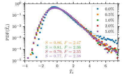
Figure 21: Histogram of the $\widetilde{T}_{\mathrm{e}}$ time series subject to outlier removal, for using different a-priori assumption for the fractions of outliers.

Even though this outlier removal procedure allows to regularize the $T_{\mathrm{e}}$ data time series, does it not allow to infer whether outlier $T_{\mathrm{e}}$ samples are due to physical events, as large temperature fluctuations, or nonphysical events, as probe arcing. The data analysis presented in this paper was performed using fit parameter time series of $I_{\mathrm{s}}$, $V_{\mathrm{f}}$, and $T_{\mathrm{e}}$ subject to a 12 point Gaussian window. Choosing this window conserves the smoothing properties of the running-average window of similar size, while at the same time it allows to avoid spurious oscillations in the high-frequency power spectral density of the time series.

References

- LaBombard et al. (2001) B. LaBombard, R. L. Boivin, M. Greenwald, J. Hughes, B. Lipschultz, D. Mossessian, C. S. Pitcher, J. L. Terry, S. J. Zweben, and the Alcator C-Mod Group (Alcator Group), Physics of Plasmas 8, 2107 (2001).
- Rudakov et al. (2002) D. L. Rudakov, J. A. Boedo, R. A. Moyer, S. Krasheninnikov, A. W. Leonard, M. A. Mahdavi, G. R. McKee, G. D. Porter, P. C. Stangeby, J. G. Watkins, W. P. West, D. G. Whyte, and G. Antar, Plasma Physics and Controlled Fusion 44, 717 (2002).
- Boedo et al. (2003) J. A. Boedo, D. L. Rudakov, R. A. Moyer, G. R. McKee, R. J. Colchin, M. J. Schaffer, P. G. Stangeby, W. P. West, S. L. Allen, T. E. Evans, R. J. Fonck, E. M. Hollmann, S. Krasheninnikov, A. W. Leonard, W. Nevins, M. A. Mahdavi, G. D. Porter, G. R. Tynan, D. G. Whyte, and X. Xu, Physics of Plasmas 10, 1670 (2003).
- Rudakov et al. (2005) D. Rudakov, J. Boedo, R. Moyer, P. Stangeby, J. Watkins, D. Whyte, L. Zeng, N. Brooks, R. Doerner, T. Evans, M. Fenstermacher, M. Groth, E. Hollmann, S. Krasheninnikov, C. Lasnier, A. Leonard, M. Mahdavi, G. McKee, A. McLean, A. Pigarov, W. Wampler, G. Wang, W. West, and C. Wong, Nuclear Fusion 45, 1589 (2005).
- Garcia et al. (2007) O. E. Garcia, J. Horacek, R. A. Pitts, A. H. Nielsen, W. Fundamenski, V. Naulin, and J. J. Rasmussen, Nuclear Fusion 47, 667 (2007).
- Garcia et al. (2006a) O. E. Garcia, J. Horacek, R. A. Pitts, A. H. Nielsen, W. Fundamenski, J. P. Graves, V. Naulin, and J. J. Rasmussen, Plasma Physics and Controlled Fusion 48, L1 (2006a).
- Fedorczak et al. (2009) N. Fedorczak, J. Gunn, P. Ghendrih, P. Monier-Garbet, and A. Pocheau, Journal of Nuclear Materials 390–391, 368 (2009).
- Carralero et al. (2014) D. Carralero, G. Birkenmeier, H. Müller, P. Manz, P. deMarne, S. Müller, F. Reimold, U. Stroth, M. Wischmeier, E. Wolfrum, and T. A. U. Team, Nuclear Fusion 54, 123005 (2014).
- Graves et al. (2005) J. P. Graves, J. Horacek, R. A. Pitts, and K. I. Hopcraft, Plasma Physics and Controlled Fusion 47, L1 (2005).
- Antar et al. (2001) G. Y. Antar, P. Devynck, X. Garbet, and S. C. Luckhardt, Physics of Plasmas 8, 1612 (2001).
- Walkden et al. (2017) N. Walkden, A. Wynn, F. Militello, B. Lipschultz, G. Matthews, C. Guillemaut, J. Harrison, D. Moulton, and J. Contributors, Nuclear Fusion 57, 036016 (2017).
- Federici et al. (2001) G. Federici, C. Skinner, J. Brooks, J. Coad, C. Grisolia, A. Haasz, A. Hassanein, V. Philipps, C. Pitcher, J. Roth, W. Wampler, and D. Whyte, Nuclear Fusion 41, 1967 (2001).
- Loarte et al. (2007) A. Loarte, B. Lipschultz, A. Kukushkin, G. Matthews, P. Stangeby, N. Asakura, G. Counsell, G. Federici, A. Kallenbach, K. Krieger, A. Mahdavi, V. Philipps, D. Reiter, J. Roth, J. Strachan, D. Whyte, R. Doerner, T. Eich, W. Fundamenski, A. Herrmann, M. Fenstermacher, P. Ghendrih, M. Groth, A. Kirschner, S. Konoshima, B. LaBombard, P. Lang, A. Leonard, P. Monier-Garbet, R. Neu, H. Pacher, B. Pegourie, R. Pitts, S. Takamura, J. Terry, E. Tsitrone, the ITPA Scrape-off Layer, and D. P. T. Group, Nuclear Fusion 47, S203 (2007).
- Lipschultz et al. (2007a) B. Lipschultz, X. Bonnin, G. Counsell, A. Kallenbach, A. Kukushkin, K. Krieger, A. Leonard, A. Loarte, R. Neu, R. Pitts, T. Rognlien, J. Roth, C. Skinner, J. Terry, E. Tsitrone, D. Whyte, S. Zweben, N. Asakura, D. Coster, R. Doerner, R. Dux, G. Federici, M. Fenstermacher, W. Fundamenski, P. Ghendrih, A. Herrmann, J. Hu, S. Krasheninnikov, G. Kirnev, A. Kreter, V. Kurnaev, B. LaBombard, S. Lisgo, T. Nakano, N. Ohno, H. Pacher, J. Paley, Y. Pan, G. Pautasso, V. Philipps, V. Rohde, D. Rudakov, P. Stangeby, S. Takamura, T. Tanabe, Y. Yang, and S. Zhu, Nuclear Fusion 47, 1189 (2007a).
- Wenninger et al. (2017) R. Wenninger, R. Albanese, R. Ambrosino, F. Arbeiter, J. Aubert, C. Bachmann, L. Barbato, T. Barrett, M. Beckers, W. Biel, L. Boccaccini, D. Carralero, D. Coster, T. Eich, A. Fasoli, G. Federici, M. Firdaouss, J. Graves, J. Horacek, M. Kovari, S. Lanthaler, V. Loschiavo, C. Lowry, H. Lux, G. Maddaluno, F. Maviglia, R. Mitteau, R. Neu, D. Pfefferle, K. Schmid, M. Siccinio, B. Sieglin, C. Silva, A. Snicker, F. Subba, J. Varje, and H. Zohm, Nuclear Fusion 57, 046002 (2017).
- Krasheninnikov (2001) S. I. Krasheninnikov, Physics Letters A 283, 368 (2001).
- D’Ippolito et al. (2002) D. A. D’Ippolito, J. R. Myra, and S. I. Krasheninnikov, Physics of Plasmas 9, 222 (2002).
- Bian et al. (2003) N. Bian, S. Benkadda, J.-V. Paulsen, and O. E. Garcia, Physics of Plasmas 10, 671 (2003).
- Yu and Krasheninnikov (2003) G. Q. Yu and S. I. Krasheninnikov, Physics of Plasmas 10, 4413 (2003).
- Myra et al. (2004) J. R. Myra, D. A. D’Ippolito, S. I. Krasheninnikov, and G. Q. Yu, Physics of Plasmas 11, 4267 (2004).
- Aydemir (2005) A. Y. Aydemir, Physics of Plasmas 12, 062503 (2005).
- Garcia et al. (2006b) O. E. Garcia, N. H. Bian, and W. Fundamenski, Physics of Plasmas 13, 082309 (2006b).
- Antar et al. (2003) G. Y. Antar, G. Counsell, Y. Yu, B. LaBombard, and P. Devynck, Physics of Plasmas 10, 419 (2003).
- Xu et al. (2005) Y. H. Xu, S. Jachmich, R. R. Weynants, and the TEXTOR team, Plasma Physics and Controlled Fusion 47, 1841 (2005).
- Garcia et al. (2013a) O. E. Garcia, S. M. Fritzner, R. Kube, I. Cziegler, B. LaBombard, and J. L. Terry, Phys. Plasmas 20, 055901 (2013a).
- Kube et al. (2016) R. Kube, A. Theodorsen, O. E. Garcia, B. LaBombard, and J. L. Terry, Plasma Physics and Controlled Fusion 58, 054001 (2016).
- Theodorsen and Garcia (2016) A. Theodorsen and O. E. Garcia, Physics of Plasmas 23, 040702 (2016).
- Theodorsen et al. (2017a) A. Theodorsen, O. Garcia, R. Kube, B. LaBombard, and J. Terry, Nuclear Fusion 57, 114004 (2017a).
- Garcia et al. (2016a) O. E. Garcia, R. Kube, A. Theodorsen, J.-G. Bak, S.-H. Hong, H.-S. Kim, the KSTAR Project Team, and R. Pitts, Nuclear Materials and Energy , (2016a).
- Ghendrih et al. (2003) P. Ghendrih, Y. Sarazin, G. Attuel, S. Benkadda, P. Beyer, G. Falchetto, C. Figarella, X. Garbet, V. Grandgirard, and M. Ottaviani, Nuclear Fusion 43, 1013 (2003).
- Garcia et al. (2004) O. E. Garcia, V. Naulin, A. H. Nielsen, and J. J. Rasmussen, Phys. Rev. Lett. 92, 165003 (2004).
- Bisai et al. (2005) N. Bisai, A. Das, S. Deshpande, R. Jha, P. Kaw, A. Sen, and R. Singh, Physics of Plasmas 12, 102515 (2005).
- Militello et al. (2012) F. Militello, W. Fundamenski, V. Naulin, and A. H. Nielsen, Plasma Physics and Controlled Fusion 54, 095011 (2012).
- Terry et al. (2003) J. L. Terry, S. J. Zweben, K. Hallatschek, B. LaBombard, R. J. Maqueda, B. Bai, C. J. Boswell, M. Greenwald, D. Kopon, W. M. Nevins, C. S. Pitcher, B. N. Rogers, D. P. Stotler, and X. Q. Xu, Physics of Plasmas 10, 1739 (2003).
- Zweben et al. (2004) S. Zweben, R. Maqueda, D. Stotler, A. Keesee, J. Boedo, C. Bush, S. Kaye, B. LeBlanc, J. Lowrance, V. Mastrocola, R. Maingi, N. Nishino, G. Renda, D. Swain, J. Wilgen, and the NSTX Team, Nuclear Fusion 44, 134 (2004).
- Terry et al. (2005) J. Terry, N. Basse, I. Cziegler, M. Greenwald, O. Grulke, B. LaBombard, S. Zweben, E. Edlund, J. Hughes, L. Lin, Y. Lin, M. Porkolab, M. Sampsell, B. Veto, and S. Wukitch, Nuclear Fusion 45, 1321 (2005).
- Zweben et al. (2006) S. J. Zweben, R. J. Maqueda, J. L. Terry, T. Munsat, J. R. Myra, D. D’Ippolito, D. A. Russell, J. A. Krommes, B. LeBlanc, T. Stoltzfus-Dueck, D. P. Stotler, K. M. Williams, C. E. Bush, R. Maingi, O. Grulke, S. A. Sabbagh, and A. E. White, Physics of Plasmas 13, 056114 (2006).
- Agostini et al. (2011) M. Agostini, J. Terry, P. Scarin, and S. Zweben, Nuclear Fusion 51, 053020 (2011).
- Maqueda et al. (2011) R. Maqueda, D. Stotler, and S. Zweben, Journal of Nuclear Materials 415, S459 (2011).
- Kube et al. (2013) R. Kube, O. Garcia, B. LaBombard, J. Terry, and S. Zweben, Journal of Nuclear Materials 438, Supplement, S505 (2013).
- Labit et al. (2007) B. Labit, I. Furno, A. Fasoli, A. Diallo, S. H. Müller, G. Plyushchev, M. Podestà, and F. M. Poli, Phys. Rev. Lett. 98, 255002 (2007).
- Sattin et al. (2009) F. Sattin, M. Agostini, R. Cavazzana, P. Scarin, and J. L. Terry, Plasma Physics and Controlled Fusion 51, 095004 (2009).
- Banerjee et al. (2012) S. Banerjee, H. Zushi, N. Nishino, K. Hanada, S. Sharma, H. Honma, S. Tashima, T. Inoue, K. Nakamura, H. Idei, M. Hasegawa, and A. Fujisawa, Nuclear Fusion 52, 123016 (2012).
- Garcia et al. (2013b) O. Garcia, I. Cziegler, R. Kube, B. LaBombard, and J. Terry, Journal of Nuclear Materials 438, S180 (2013b).
- Banerjee et al. (2014) S. Banerjee, H. Zushi, N. Nishino, K. Hanada, M. Ishiguro, S. Tashima, H. Q. Liu, K. Mishra, K. Nakamura, H. Idei, M. Hasegawa, A. Fujisawa, Y. Nagashima, and K. Matsuoka, Physics of Plasmas 21, 072311 (2014).
- Theodorsen et al. (2016) A. Theodorsen, O. E. Garcia, J. Horacek, R. Kube, and R. A. Pitts, Plasma Physics and Controlled Fusion 58, 044006 (2016).
- Garcia et al. (2016b) O. E. Garcia, R. Kube, A. Theodorsen, and H. L. Pécseli, Physics of Plasmas 23, 052308 (2016b).
- Silva et al. (2009) C. Silva, W. Fundamenski, A. Alonso, B. Gonçalves, C. Hidalgo, M. A. Pedrosa, R. A. Pitts, M. Stamp, and J. E. contributors, Plasma Physics and Controlled Fusion 51, 105001 (2009).
- Tanaka et al. (2015) H. Tanaka, S. Masuzaki, N. Ohno, T. Morisaki, and Y. Tsuji, Journal of Nuclear Materials 463, 761 (2015).
- Grulke et al. (2006) O. Grulke, J. L. Terry, B. LaBombard, and S. J. Zweben, Physics of Plasmas 13, 012306 (2006).
- Saha and Chowdhury (2008) S. K. Saha and S. Chowdhury, Physics of Plasmas 15, 012305 (2008).
- Garcia (2012) O. E. Garcia, Phys. Rev. Lett. 108, 265001 (2012).
- Garcia et al. (2015) O. E. Garcia, J. Horacek, and R. A. Pitts, Nuclear Fusion 55, 062002 (2015).
- Militello and Omotani (2016) F. Militello and J. Omotani, Nuclear Fusion 56, 104004 (2016).
- Theodorsen et al. (2017b) A. Theodorsen, O. E. Garcia, and M. Rypdal, Physica Scripta 92, 054002 (2017b).
- Garcia and Theodorsen (2017) O. E. Garcia and A. Theodorsen, Physics of Plasmas 24, 032309 (2017).
- Mekkaoui (2013) A. Mekkaoui, Physics of Plasmas (1994-present) 20, 010701 (2013).
- Müller et al. (2010) H. Müller, J. Adamek, J. Horacek, C. Ionita, F. Mehlmann, V. Rohde, R. Schrittwieser, and A. U. Team, Contributions to Plasma Physics 50, 847 (2010).
- Hutchinson (2000) I. Hutchinson, Principles of Plasma Diagnostics, 2nd ed. (Cambridge University Press, 2000).
- Stangeby (2000) P. C. Stangeby, The Plasma Boundary Of Magnetic Fusion Devices (IoP Publishing, 2000).
- Rohde (1996) V. Rohde, Contributions to Plasma Physics 36, 109 (1996).
- Horacek et al. (2010) J. Horacek, J. Adamek, H. Müller, J. Seidl, A. Nielsen, V. Rohde, F. Mehlmann, C. Ionita, E. Havlíčková, and the ASDEX Upgrade Team, Nuclear Fusion 50, 105001 (2010).
- Nold et al. (2012) B. Nold, T. T. Ribeiro, M. Ramisch, Z. Huang, H. W. Müller, B. D. Scott, U. Stroth, and the ASDEX Upgrade Team, New Journal of Physics 14, 063022 (2012).
- Gennrich and Kendl (2012) F. P. Gennrich and A. Kendl, Plasma Physics and Controlled Fusion 54, 015012 (2012).
- Adámek et al. (2004) J. Adámek, J. Stöckel, M. Hron, J. Ryszawy, M. Tichý, R. Schrittwieser, C. Ionită, P. Balan, E. Martines, and G. V. Oost, Czechoslovak Journal of Physics 54, C95 (2004).
- Adámek et al. (2009) J. Adámek, V. Rohde, H. Müller, A. Herrmann, C. Ionita, R. Schrittwieser, F. Mehlmann, J. Stöckel, J. Horacek, J. Brotankova, and A. U. Team, Journal of Nuclear Materials 390–391, 1114 (2009).
- Schrittwieser et al. (2002) R. Schrittwieser, J. Adámek, P. Balan, M. Hron, C. Ionita, K. Jakubka, L. Kryska, E. Martines, J. Stöckel, M. Tichy, and G. V. Oost, Plasma Physics and Controlled Fusion 44, 567 (2002).
- Schrittwieser et al. (2008) R. Schrittwieser, C. Ionita, P. Balan, C. Silva, H. Figueiredo, C. A. F. Varandas, J. J. Rasmussen, and V. Naulin, Plasma Physics and Controlled Fusion 50, 055004 (2008).
- Ionita et al. (2011) C. Ionita, J. Grünwald, C. Maszl, R. Stärz, M. Čerček, B. Fonda, T. Gyergyek, G. Filipič, J. Kovačič, C. Silva, H. Figueiredo, T. Windisch, O. Grulke, T. Klinger, and R. Schrittwieser, Contributions to Plasma Physics 51, 264 (2011).
- Adamek et al. (2014) J. Adamek, J. Horacek, J. Seidl, H. W. Müller, R. Schrittwieser, F. Mehlmann, P. Vondracek, S. Ptak, C. Team, and A. U. Team, Contributions to Plasma Physics 54, 279 (2014).
- Lin et al. (1992) H. Lin, G. X. Li, R. D. Bengtson, C. P. Ritz, and H. Y. W. Tsui, Review of Scientific Instruments 63, 4611 (1992).
- Asakura et al. (1995) N. Asakura, S. Tsuji‐Iio, Y. Ikeda, Y. Neyatani, and M. Seki, Review of Scientific Instruments 66, 5428 (1995).
- Yang et al. (2003) Y. Yang, G. Counsell, and T. M. team, Journal of Nuclear Materials 313-316, 734 (2003), plasma-Surface Interactions in Controlled Fusion Devices 15.
- Kim et al. (2016) H.-S. Kim, J.-G. Bak, M.-K. Bae, K.-S. Chung, and S.-H. Hong, Fusion Engineering and Design 109-111, 809 (2016), proceedings of the 12th International Symposium on Fusion Nuclear Technology-12 (ISFNT-12).
- Meier et al. (1995) M. A. Meier, G. A. Hallock, H. Y. W. Tsui, and R. D. Bengtson, Review of Scientific Instruments 66, 437 (1995), https://doi.org/10.1063/1.1146372 .
- Meier et al. (1997) M. A. Meier, G. A. Hallock, and R. D. Bengtson, Review of Scientific Instruments 68, 369 (1997).
- Meier et al. (2001) M. A. Meier, R. D. Bengtson, G. A. Hallock, and A. J. Wootton, Phys. Rev. Lett. 87, 085003 (2001).
- Boedo et al. (1999) J. A. Boedo, D. Gray, R. W. Conn, P. Luong, M. Schaffer, R. S. Ivanov, A. V. Chernilevsky, G. V. Oost, and T. T. Team, Review of Scientific Instruments 70, 2997 (1999).
- Labombard and Lyons (2007) B. Labombard and L. Lyons, Review of Scientific Instruments 78, 073501 (2007).
- LaBombard et al. (2014) B. LaBombard, T. Golfinopoulos, J. L. Terry, D. Brunner, E. Davis, M. Greenwald, and J. W. Hughes, Physics of Plasmas 21, 056108 (2014).
- Hutchinson et al. (1994) I. H. Hutchinson, R. Boivin, F. Bombarda, P. Bonoli, S. Fairfax, C. Fiore, J. Goetz, S. Golovato, R. Granetz, M. Greenwald, S. Horne, A. Hubbard, J. Irby, B. LaBombard, B. Lipschultz, E. Marmar, G. McCracken, M. Porkolab, J. Rice, J. Snipes, Y. Takase, J. Terry, S. Wolfe, C. Christensen, D. Garnier, M. Graf, T. Hsu, T. Luke, M. May, A. Niemczewski, G. Tinios, J. Schachter, and J. Urbahn, Physics of Plasmas 1, 1511 (1994).
- Greenwald et al. (2013) M. Greenwald, A. Bader, S. Baek, H. Barnard, W. Beck, W. Bergerson, I. Bespamyatnov, M. Bitter, P. Bonoli, M. Brookman, D. Brower, D. Brunner, W. Burke, J. Candy, M. Chilenski, M. Chung, M. Churchill, I. Cziegler, E. Davis, G. Dekow, L. Delgado-Aparicio, A. Diallo, W. Ding, A. Dominguez, R. Ellis, P. Ennever, D. Ernst, I. Faust, C. Fiore, E. Fitzgerald, T. Fredian, O. Garcia, C. Gao, M. Garrett, T. Golfinopoulos, R. Granetz, R. Groebner, S. Harrison, R. Harvey, Z. Hartwig, K. Hill, J. Hillairet, N. Howard, A. Hubbard, J. Hughes, I. Hutchinson, J. Irby, A. James, A. Kanojia, C. Kasten, J. Kesner, C. Kessel, R. Kube, B. LaBombard, C. Lau, J. Lee, K. Liao, Y. Lin, B. Lipschultz, Y. Ma, E. Marmar, P. McGibbon, O. Meneghini, D. Mikkelsen, D. Miller, R. Mumgaard, R. Murray, R. Ochoukov, G. Olynyk, D. Pace, S. Park, R. Parker, Y. Podpaly, M. Porkolab, M. Preynas, I. Pusztai, M. Reinke, J. Rice, W. Rowan, S. Scott, S. Shiraiwa, J. Sierchio, P. Snyder, B. Sorbom, V. Soukhanovskii, J. Stillerman, L. Sugiyama, C. Sung, D. Terry, J. Terry, C. Theiler, N. Tsujii, R. Vieira, J. Walk, G. Wallace, A. White, D. Whyte, J. Wilson, S. Wolfe, K. Woller, G. Wright, J. Wright, S. Wukitch, G. Wurden, P. Xu, C. Yang, and S. Zweben, Nuclear Fusion 53, 104004 (2013).
- Greenwald et al. (2014) M. Greenwald, A. Bader, S. Baek, M. Bakhtiari, H. Barnard, W. Beck, W. Bergerson, I. Bespamyatnov, P. Bonoli, D. Brower, D. Brunner, W. Burke, J. Candy, M. Churchill, I. Cziegler, A. Diallo, A. Dominguez, B. Duval, E. Edlund, P. Ennever, D. Ernst, I. Faust, C. Fiore, T. Fredian, O. Garcia, C. Gao, J. Goetz, T. Golfinopoulos, R. Granetz, O. Grulke, Z. Hartwig, S. Horne, N. Howard, A. Hubbard, J. Hughes, I. Hutchinson, J. Irby, V. Izzo, C. Kessel, B. LaBombard, C. Lau, C. Li, Y. Lin, B. Lipschultz, A. Loarte, E. Marmar, A. Mazurenko, G. McCracken, R. McDermott, O. Meneghini, D. Mikkelsen, D. Mossessian, R. Mumgaard, J. Myra, E. Nelson-Melby, R. Ochoukov, G. Olynyk, R. Parker, S. Pitcher, Y. Podpaly, M. Porkolab, M. Reinke, J. Rice, W. Rowan, A. Schmidt, S. Scott, S. Shiraiwa, J. Sierchio, N. Smick, J. A. Snipes, P. Snyder, B. Sorbom, J. Stillerman, C. Sung, Y. Takase, V. Tang, J. Terry, D. Terry, C. Theiler, A. Tronchin-James, N. Tsujii, R. Vieira, J. Walk, G. Wallace, A. White, D. Whyte, J. Wilson, S. Wolfe, G. Wright, J. Wright, S. Wukitch, and S. Zweben, Physics of Plasmas 21, 110501 (2014).
- Lipschultz et al. (2007b) B. Lipschultz, B. LaBombard, J. L. Terry, C. Boswell, and I. H. Hutchinson, Fusion Science and Technology 51, 369 (2007b), http://dx.doi.org/10.13182/FST07-A1428 .
- Smick and LaBombard (2009) N. Smick and B. LaBombard, Review of Scientific Instruments 80, 023502 (2009).
- Pécseli and Trulsen (1989) H. L. Pécseli and J. Trulsen, Physics of Fluids B: Plasma Physics (1989-1993) 1, 1616 (1989).
- Theodorsen and Garcia (2018) A. Theodorsen and O. E. Garcia, Plasma Physics and Controlled Fusion 60, 034006 (2018).
- Øynes et al. (1995) F. J. Øynes, H. L. Pécseli, and K. Rypdal, Phys. Rev. Lett. 75, 81 (1995).
- Zweben et al. (2002) S. J. Zweben, D. P. Stotler, J. L. Terry, B. LaBombard, M. Greenwald, M. Muterspaugh, C. S. Pitcher, K. Hallatschek, R. J. Maqueda, B. Rogers, J. L. Lowrance, V. J. Mastrocola, and G. F. Renda, Physics of Plasmas 9, 1981 (2002).
- Stotler et al. (2003) D. Stotler, B. LaBombard, J. Terry, and S. Zweben, Journal of Nuclear Materials 313–316, 1066 (2003).
- Marandet et al. (2016) Y. Marandet, N. Nace, M. Valentinuzzi, P. Tamain, H. Bufferand, G. Ciraolo, P. Genesio, and N. Mellet, Plasma Physics and Controlled Fusion 58, 114001 (2016).
- Naujoks (2006) D. Naujoks, Plasma-Material Interaction in Controlled Fusion (Springer, 2006).
- Bohdansky (1984) J. Bohdansky, Nuclear Instruments and Methods in Physics Research Section B: Beam Interactions with Materials and Atoms 2, 587 (1984).
- Garcia et al. (2006c) O. E. Garcia, J. Horacek, R. A. Pitts, A. H. Nielsen, W. Fundamenski, J. P. Graves, V. Naulin, and J. J. Rasmussen, Plasma Physics and Controlled Fusion 48, L1 (2006c).
- Fedorczak et al. (2011) N. Fedorczak, J. Gunn, P. Ghendrih, G. Ciraolo, H. Bufferand, L. Isoardi, P. Tamain, and P. Monier-Garbet, Journal of Nuclear Materials 415, S467 (2011).
- Ghendrih et al. (2005) P. Ghendrih, Y. Sarazin, G. Attuel, S. Benkadda, P. Beyer, G. Darmet, G. Falchetto, C. Figarella, X. Garbet, V. Grandgirard, and M. Ottaviani, Journal of Nuclear Materials 337–339, 347 (2005).
- Katz et al. (2008) N. Katz, J. Egedal, W. Fox, A. Le, and M. Porkolab, Phys. Rev. Lett. 101, 015003 (2008).
- Furno et al. (2011) I. Furno, C. Theiler, D. Lançon, A. Fasoli, D. Iraji, P. Ricci, M. Spolaore, and N. Vianello, Plasma Physics and Controlled Fusion 53, 124016 (2011).
- Theiler et al. (2011) C. Theiler, I. Furno, A. Fasoli, P. Ricci, B. Labit, and D. Iraji, Physics of Plasmas 18, 055901 (2011).
- Wiesenberger et al. (2014) M. Wiesenberger, J. Madsen, and A. Kendl, Physics of Plasmas 21, 092301 (2014).
- Held et al. (2016) M. Held, M. Wiesenberger, J. Madsen, and A. Kendl, Nuclear Fusion 56, 126005 (2016).
- D’Ippolito et al. (2004) D. A. D’Ippolito, J. R. Myra, S. I. Krasheninnikov, G. Q. Yu, and A. Y. Pigarov, Contributions to Plasma Physics 44, 205 (2004).
- Militello et al. (2013) F. Militello, P. Tamain, W. Fundamenski, A. Kirk, V. Naulin, A. H. Nielsen, and the MAST team, Plasma Physics and Controlled Fusion 55, 025005 (2013).
- Liu et al. (2012) F. T. Liu, K. M. Ting, and Z.-H. Zhou, ACM Trans. Knowl. Discov. Data 6, 3:1 (2012).
- Pedregosa et al. (2011) F. Pedregosa, G. Varoquaux, A. Gramfort, V. Michel, B. Thirion, O. Grisel, M. Blondel, P. Prettenhofer, R. Weiss, V. Dubourg, J. Vanderplas, A. Passos, D. Cournapeau, M. Brucher, M. Perrot, and E. Duchesnay, Journal of Machine Learning Research 12, 2825 (2011).
- (106) NIST/SEMATECH, “e-handbook of statistical methods, http://itl.nist.gov/div898/handbook, 2017-09,” .